| Issue |
A&A
Volume 690, October 2024
|
|
|---|---|---|
| Article Number | A40 | |
| Number of page(s) | 12 | |
| Section | Cosmology (including clusters of galaxies) | |
| DOI | https://doi.org/10.1051/0004-6361/202450512 | |
| Published online | 27 September 2024 | |
Model-independent cosmographic constraints from DESI 2024
1
Università di Camerino, Divisione di Fisica,
Via Madonna delle carceri 9,
62032
Camerino,
Italy
2
SUNY Polytechnic Institute,
Utica,
NY
13502,
USA
3
INFN, Sezione di Perugia,
Perugia
06123,
Italy
4
INAF – Osservatorio Astronomico di Brera,
Milano,
Italy
5
Al-Farabi Kazakh National University,
Al-Farabi av. 71,
050040
Almaty,
Kazakhstan
6
ICRANet,
P.zza della Repubblica 10,
65122
Pescara,
Italy
e-mail: This email address is being protected from spambots. You need JavaScript enabled to view it.
Received:
25
April
2024
Accepted:
24
June
2024
Abstract
Context. We explore model-independent constraints on the Universe kinematics up to the snap and jerk hierarchical terms, considering the latest baryon acoustic oscillation (BAO) release provided by the DESI collaboration.
Aims. We intend to place novel and more stringent constraints on the cosmographic series, incorporating three combinations of data catalogs: the first made by BAO and observational cosmic chronometers, the second made by BAO and type Ia supernovae, and the last including all the cited data sets.
Methods. Considering the latest BAO data provided by the DESI collaboration and tackling the rd parameter to span within the range [144,152] Mpc, with a fixed step of δrd = 2 Mpc, we employed Monte Carlo Markov chain analyses based on the Metropolis algorithm to fix novel bounds on the cosmographic series, fixing the deceleration, q0 , the jerk, j0 , and the snap, s0, parameters, up to the 2σ level. A comparison between the results of the Planck satellite with those obtained by the DESI collaboration is also reported.
Results. Our findings showcase a significant departure in terms of j0 even at the 1σ confidence level, albeit compatible with the ACDM paradigm in regard to q0 and s0 at the 2σ level. Analogously, the h0 tension appears alleviated in the second hierarchy when including snap.
Conclusions. Our method excludes models that significantly depart from the standard cosmological model. Particularly, direct comparisons with the ACDM and wCDM models and the Chevallier-Polarski-Linder parameterisation are explored, which definitively favour the wCDM scenario over other approaches, contradicting the findings of the original DESI collaboration.
Key words: cosmological parameters / cosmology: theory / dark energy / distance scale / large-scale structure of Universe
Corresponding author; This email address is being protected from spambots. You need JavaScript enabled to view it.
© The Authors 2024
 Open Access article, published by EDP Sciences, under the terms of the Creative Commons Attribution License (https://creativecommons.org/licenses/by/4.0), which permits unrestricted use, distribution, and reproduction in any medium, provided the original work is properly cited.
This article is published in open access under the Subscribe to Open model. This email address is being protected from spambots. You need JavaScript enabled to view it. to support open access publication.
1 Introduction
The cosmological concordance model predicts the existence of a cosmological constant, Λ, in the well-established ΛCDM paradigm, which is quite robustly supported by several cosmological observations (Copeland et al. 2006). However, the recent DESI map (DESI Collaboration 2024) provides an analysis of the underlying structure of the Universe with higher precision than previous missions, showing results that, if confirmed, may suggest a possible deviation from our present understanding of dark energy. Accordingly, the recent experimental results obtained by the Planck satellite (Planck Collaboration VI 2020) and developments of dark energy evolution have been brought into question.
More specifically, DESI measures the characteristic separation of galaxies, namely the baryonic acoustic oscillation (BAO). From these analyses, an apparent tension with the standard cosmological model has been found with a confidence level of up to 3.9σ, suggesting the existence of a possible slightly evolving dark energy contribution, departing from the pure cosmological constant, Λ1.
Although DESI seeks to answer the question of whether or not dark energy has a constant value everywhere in the Universe, and is therefore a cosmological constant, its results are based on assuming a given cosmological model a priori, leading to a possible degeneracy problem. In other words, more than one model can explain dynamical dark energy.
Although we might be tempted, we cannot be sure that the ΛCDM model is no longer suitable until we look at the next batch of data, and it still appears to be the best suite to describe the overall dynamics. Indeed, due to the plethora of contrasting cosmological scenarios (Weinberg 1989; Tsujikawa 2011), the use of model-independent treatments to frame the Universe dynamics becomes decisive to single out the most suitable cosmological model (Sahni & Starobinsky 2006; Kunz 2012). Among others, a powerful example of a model-independent treatment is offered by cosmography (Weinberg 1972; Harrison 1976; Landsberg & Pathria 1974; Visser 1997), where Taylor series involving expansions of a(t) and/or cosmic distances around our time (Visser 2005; Luongo 2011, 2013) are directly compared with cosmic data (Visser 2015), without the need to fix a cosmological model a priori (Visser 2005; Bargiacchi et al. 2023; Aviles et al. 2013b; Luongo & Quevedo 2014b; Capozziello et al. 2017, 2022). However, although we can apply cosmography to different contexts (see e.g. Calzá et al. 2020; Capozziello et al. 2015, 2014, 2018b; de la Cruz-Dombriz et al. 2016; Aviles et al. 2013a,b; Luongo & Muccino 2021, 2023; Izzo et al. 2012), it may produce inconclusive numerical results because of intrinsic problems of convergence and truncation (Luongo & Quevedo 2014a; Aviles & Cervantes-Cota 2011; Kunz et al. 2006; Luongo et al. 2016). The need for further data points is therefore essential in the realm of cosmographic expansions and, in this respect, the DESI measurements can significantly refine the cosmographic analysis, as we show in the present work.
Motivated by the above points, we analysed 30 modelindependent constraints of the kinematics of the Universe: that is, the first set of 15 bounds up to the jerk parameter, corresponding to the third expansion order of the luminosity distance, and the second set of 15 fits up to the further order, including the snap parameter. To do so, we performed a Monte Carlo Markov chain (MCMC) set of analyses, employing the most recent BAO measurements inferred by the DESI collaboration.
Particularly, the sound horizon at the drag epoch associated with BAO data, rd, is compatible with the results found by the Planck satellite and by the DESI collaboration, respectively.
Precisely, in our fits, we assume it to span the discrete interval rd ∈ [144,152] Mpc with a step of δrd = 2 Mpc. In such a way, we put stringent bounds on the cosmographic series, verifying the findings made by the DESI mission in a modelindependent way. Accordingly, our findings are obtained by considering a hierarchy among cosmic data points. First, we consider the BAO points with the observational Hubble data (OHD), and then we combine BAO points with the type Ia supernovae (SNe Ia) of the Pantheon catalogue, before finally using a combination of all the aforementioned three data sets. We report convergent limits on the cosmographic set, including the deceleration, q0, the jerk, j0, and the snap s0 parameters, showing that they turn out to be fully constrained at 1σ. We obtain very tight errors on the first hierarchy up to the jerk parameter, and then we compare our findings with dark energy models, such as the ΛCDM paradigm, the wCDM, and the Chevallier-Polarski- Linder (CPL) parametrisation. We conclude that dynamical dark energy is better adapted to this catalogue of BAO, because the concordance model exhibits severe departures, mainly regarding the jerk parameter. The consequences of these findings for the onset of cosmic acceleration and for how to alleviate the cosmological tension regarding h0 are then discussed.
The paper is structured as follows. In Sect. 2, we introduce the theoretical model-independent expansions that we want to constrain. In Sect. 3, we report our numerical outcomes and analyse the corresponding bounds; the physical consequences of our analyses are also discussed. Conclusions and a final outlook are reported in Sect. 4, together with the perspectives of our work.
2 Theoretical scenario
In a homogeneous, isotropic, and spatially flat universe, the corresponding Friedmann, Lemaître, Robertson, and Walker line element ds2 = dt2 − a(t)2 [dr2 + r2 dl2], with dl2 ≡ (dθ2 + sin2 θ dϕ2), implies the presence of a single scale factor a(t), conventionally normalised to unity. With this metric, the Einstein equations provide the dynamical Friedmann equations:
 (1)
(1)
where H is the Hubble rate, and ρ and P are the energy density and pressure of the total cosmic fluid, respectively.
After defining the cosmological densities ρi as ratios Ωi ≡ ρi /ρc, normalised to the critical density  , the cosmological content is well approximated by dust matter and dark energy at late times, neglecting further fluids, such as radiation, neutrinos, and so on.
The cosmological information is incorporated into the Hubble rate. Thus, to feature a model-independent strategy to fix cosmic bounds, one can directly expand the scale factor in Taylor series around the present time in order to fix the derivatives of a(t) at the our time. This treatment is called the cosmographic technique, and entails a model-independent investigation of the kinematic variables without taking into account any cosmological model a priori (Dunsby & Luongo 2016).
Cosmography appears particularly interesting in view of the recent findings of the DESI collaboration, where dynamical dark energy has not been fully excluded and an evident tension with previous studies is highlighted (DESI Collaboration 2024).
In particular, following the cosmographic recipe, we have
 (2)
(2)
where conventionally we truncated the series up to a given order, having at all times (Cattoën & Visser 2008)
 (3)
(3)
as coefficients of the above expansion, in general known as deceleration q, jerk j, and snap s parameters.
Bearing the above considerations in mind and relating a(t) to the redshift z, we then write the Hubble parameter as a function of the luminosity distance dL(z) as
![Mathematical equation: $H(z) = {\left[ {{d \over {dz}}\left( {{{{d_L}(z)} \over {1 + z}}} \right)} \right]^{ - 1}},$](/articles/aa/full_html/2024/10/aa50512-24/aa50512-24-eq5.png) (4)
(4)
immediately yielding
 (5)
(5)
where the coefficients αn and Hm can be found in Capozziello et al. (2019) and Capozziello et al. (2020). The corresponding truncated series suffer from several problems, among which are the order truncation and the convergence problem (Dunsby & Luongo 2016; Gruber & Luongo 2014; Bamba et al. 2012).
In an attempt to alleviate these issues, different hierarchies among data sets and orders of the employed series can be con- sidered2. The orders and hierarchies that we consider here are (1) up to the jerk parameter first, and then (2) up to the snap parameter, all compared with three combinations of data sets in the following order,
BAO+OHD,
BAO+SNe Ia,
BAO+OHD+SNe Ia.
We note that the two orders invoked here minimally characterise possible deviations from the standard cosmological model. Indeed, to identify a given model, we need to compute the Taylor series up to the snap parameter, whereas the analysis performed up to the jerk is considered to check possible departures in terms of j0 with respect to the further order in s0 .
For our subsequent purposes, it is now convenient to compute the cosmographic series for three given models of dark energy. Precisely, with Ωm(z) ≡ Ωm(1 + z)3, we focus on the following models:
-
The standard ΛCDM model, with normalised Hubble rate
 . The only model parameter is Ωm, where Ωλ = 1 − Ωm, providing the current cosmographic set3,
 (6a)
(6a)
 (6b)
(6b)
 (6c)
(6c)As an example that we use below, in a perfect concordance scenario, say Ωm = 0.3, we obtain
 (7)
(7) -
The wCDM model, in analogy to the ΛCDM model. The wCDM has a negative barotropic factor likely due to a dynamical, slowly rolling scalar field, and has two parameters, Ωm and w, the normalised Hubble rate
 , with ΩX = 1 − Ωm, and
![Mathematical equation: ${q_0} = {1 \over 2}\left[ {1 - 3w\left( {{{\rm{\Omega }}_m} - 1} \right)} \right],$](/articles/aa/full_html/2024/10/aa50512-24/aa50512-24-eq19.png) (8a)
(8a)
![Mathematical equation: ${j_0} = {1 \over 2}\left[ {2 - 9w\left( {{{\rm{\Omega }}_m} - 1} \right)(1 + w)} \right],$](/articles/aa/full_html/2024/10/aa50512-24/aa50512-24-eq20.png) (8b)
(8b)
![Mathematical equation: $\matrix{ {{s_0} = - {7 \over 2} + {9 \over 4}\left( {{{\rm{\Omega }}_m} - 1} \right)w[9 + w(16 + 9w} \hfill \cr {\,\,\,\,\,\,\,\,\,\,\, - 3{{\rm{\Omega }}_m}(1 + w))].} \hfill \cr } $](/articles/aa/full_html/2024/10/aa50512-24/aa50512-24-eq21.png) (8c)
(8c)Again, in a genuine scenario, with arbitrary Ωm = 0.3 and w = −9/10, we have
 (9)
(9) -
The CPL parameterisation, sometimes referred to as the w0waCDM model. This model was originally found as a first- order Taylor expansion around a = 1 of the barotropic factor ω(z) = ω0 + ωaz/(1 + z), and suggests a normalised Hubble rate,
 (10)
(10)where Ωm, ω0, and ωa are the three free model parameters, yielding a statistically more complicated model than the previous two. We thus write
![Mathematical equation: ${q_0} = {1 \over 2}\left[ {1 - 3{\omega _0}\left( {{{\rm{\Omega }}_m} - 1} \right)} \right],$](/articles/aa/full_html/2024/10/aa50512-24/aa50512-24-eq24.png) (11a)
(11a)
![Mathematical equation: ${j_0} = {1 \over 2}\left[ {2 - 9{\omega _0}\left( {{{\rm{\Omega }}_m} - 1} \right)\left( {1 + {\omega _0}} \right) + 3{\omega _a} - 3{{\rm{\Omega }}_m}{\omega _a}} \right]{\rm{,}}$](/articles/aa/full_html/2024/10/aa50512-24/aa50512-24-eq25.png) (11b)
(11b)
![Mathematical equation: $\matrix{ {{s_0} = {1 \over 4}\{ - 14 - 9\left( { - 1 + {{\rm{\Omega }}_m}} \right){w_0}[ - 9 + {w_0}( - 16 - 9{w_0}} \cr { + 3{{\rm{\Omega }}_m}\left( {1 + {w_0}} \right))] - 33{w_a} + 33{{\rm{\Omega }}_m}{w_a}} \cr { - 9\left( { - 7 + {{\rm{\Omega }}_m}} \right)\left( { - 1 + {{\rm{\Omega }}_m}} \right){w_0}{w_a}\} .} \cr } $](/articles/aa/full_html/2024/10/aa50512-24/aa50512-24-eq26.png) (11c)
(11c)Analogously, with Ωm = 0.3, w0 = −9/10, and wa = 0.5, we obtain
 (12)
(12)
The values reported in Eqs. (7), (9), and (12) are compatible with experimental results performed on them (Dunsby & Luongo 2016). However, more precise values are found in Table 1, where we compute the cosmographic set through the bounds inferred from the Planck satellite and DESI measurements, respectively. Nevertheless, we now have all the ingredients to directly compare the truncated series in Eq. (2) with data and then to check the agreement of our results with the DESI outcomes. Further, we also compare our expectations in Table 1 with the cosmographic results.
Theoretical cosmographic coefficients.
3 Numerical analysis
We combine the DESI−BAO measurements – that is, the fixed catalogue – with standard low−redshift data surveys. Precisely, we consider the OHD (Moresco et al. 2022) and the Pantheon catalogue of SNe Ia (Scolnic et al. 2018). Therefore, the general best−fit parameters are clearly determined directly by maximising the total log−likelihood function
 (13)
(13)
Clearly, the above relation represents the largest combination of likelihoods, which reduces to the sum of two terms – with the BAO likelihood always present – according to the kind of fit we perform. Below, we define the contribution of each probe.
-
DESI-BAO data. The DESI-BAO measurements are essentially galaxy surveys across seven distinct redshift bins within a total range of z ∈ [0.1, 4.2], in which all the measurements are effectively independent from each other, as noted in DESI Collaboration (2024). Accordingly, no covariance matrix is introduced here, whereas the systematic errors associated with these measurements introduce a negligible offset (DESI Collaboration 2024; Glanville et al. 2021).
Hence, the DESI-BAO data are equivalently expressed as the ratios
 (14)
(14)or only as the ratio
![Mathematical equation: ${{{d_V}(z)} \over {{r_d}}} = {{{{\left[ {zd_M^2(z){d_H}(z)} \right]}^{1/3}}} \over {{r_d}}},$](/articles/aa/full_html/2024/10/aa50512-24/aa50512-24-eq30.png) (15)
(15)when the signal-to-noise ratio is low (see Table 2).
The sound horizon at the drag epoch, rd , depends on the matter and baryon physical energy densities and the effective number of extrarelativistic degrees of freedom. In our computation, we fit rd assuming different ranges of plausibility, that is, enabling it to span within the values rd ∈ [144, 152] Mpc, within which both the Planck satellite and DESI-BAO expectations fall. In so doing, we only a posteriori extract the most viable values for rd. The procedure of fixing rd is clearly motivated by reducing the complexity of the computation. Even though a possible strategy could be to leave rd free to vary, the above-mentioned approach allows us to significantly reduce the computations without altering the final outputs.
Thus, with the assumption of Gaussian distributed errors, σXi, the log-likelihood functions for each ratio, X = dM /rd, dH /rd, dV /rd, can be written as
![Mathematical equation: $\ln {{\cal L}_{\rm{X}}} = - {1 \over 2}\mathop {\mathop \sum \nolimits^ }\limits_{i = 1}^{{N_{\rm{X}}}} \left\{ {{{\left[ {{{{X_i} - X\left( {{z_i}} \right)} \over {{\sigma _{{X_i}}}}}} \right]}^2} + \ln \left( {2\pi \sigma _{{X_j}}^2} \right)} \right\},$](/articles/aa/full_html/2024/10/aa50512-24/aa50512-24-eq31.png) (16)
(16)and the total BAO log-likelihood turns out to be
 (17)
(17) -
Hubble rate data. Here, we adopt the most updated sample of OHD, which consists of the NO = 34 measurements conventionally reported in Table 3. These measurements are of particular interest because they are determined from spectroscopic detection of the differences in age, ∆t, and redshift, ∆z, of couples of passively evolving galaxies. To do so, we assume that the underlying galaxies are nevertheless formed at the same time, enabling us to consider the identity H(z) = −(1 + z)−1∆z/∆t (Jimenez & Loeb 2002).
Consequently, the OHD systematic errors mostly depend on stellar population synthesis models and libraries. Even the initial mass functions – taken into account with the purpose of calibrating the measures – together with the stellar metallicity of the population may contribute, often with picks of further 20–30% errors (Montiel et al. 2021; Moresco et al. 2022; Muccino et al. 2023). The measurements are thus not particularly accurate, albeit their determination is fully model independent.
For the sake of simplicity, again we employ Gaussian distributed errors, σHk. Therefore, the best-fit parameters are found by maximising the log-likelihood
![Mathematical equation: $\ln {{\cal L}_{\rm{O}}} = - {1 \over 2}\mathop {\mathop \sum \nolimits^ }\limits_{i = 1}^{{N_{\rm{O}}}} \left\{ {{{\left[ {{{{H_i} - H\left( {{z_i}} \right)} \over {{\sigma _{{H_i}}}}}} \right]}^2} + \ln \left( {2\pi \sigma _{{H_i}}^2} \right)} \right\}.$](/articles/aa/full_html/2024/10/aa50512-24/aa50512-24-eq33.png) (18)
(18) -
SNe Ia. The most recent catalog of SNe data points, namely the Pantheon data set, is made up of 1048 measurements associated with SNe (Scolnic et al. 2018), although it can be significantly reduced – once the spatial curvature is assumed to be zero – to a catalog of NS = 6 measurements, reported in a practical way as normalised Hubble rates, Ei (Riess et al. 2018). Here, the corresponding log-likelihood function is given by
 (19)
(19)where we impose
 , the covariance matrix CS, and its determinant |CS |.
Data points of the OHD catalog.
3.1 Results
We worked out two different hierarchies of coefficients, up to jerk first, and then snap. In both cases, the cosmo- graphic series converge regardless of the order or the value of rd ∈ [144, 152] Mpc.
Concerning the bounds on rd and H0 , BAO measurements are sensitive to the degeneracy H0–rd (Sutherland 2012). This is evident from the fact that, in Tables 4–5, the values of H0 = 100 h0 km/s/Mpc decrease for increasing rd, whereas all the other parameters are stable and insensitive to this degeneracy, regardless of the hierarchy. In this sense, it is within our expectations that DESI-BAO+SN Ia fits – with the SN data set being based on E(z) measurements, and therefore independent of H0 – are unable to break such a degeneracy. As a result, for this set of fits, rd is absolutely unconstrained, as is h0 , although this latter aligns with Planck expectations (Planck Collaboration VI 2020).
In general, the best-fit parameters, including the comoving sound horizons at the drag epoch rd , are determined by looking at the set of model parameters furnishing the maximum value of the log-likelihood ln 𝓛, that is, when ∆ = 0.00. Excluding the DESI-BAO+SN fits, in the BAO+OHD and BAO+OHD+SN Ia combinations of data sets, the minimum ∆ is related to rd ≃ 146 Mpc for the hierarchy up to j0 , and to rd ≃ 148 Mpc for the hierarchy up to s0. The corresponding contour plots are shown in Figs. A.1–A.3.
Comparing the outcomes regarding the parameters q0, j0, and s0 with previous cosmographic bounds, it is evident that this is among the first occurrences in which the cosmographic series can always converge. From all the measurements, it appears evident that q0 < 0, s0 < 0, while j0 > 0, as theoretically predicted in Luongo (2013). However, quite surprisingly, the values of the parameters are stable regardless of the hierarchical order involved, namely in both cases and for all the data sets involved.
In particular, from the sign of q, one can infer whether or not (and by how much) the Universe is decelerating, while a positive sign of j0 indicates a transition time between the matter- and dark-energy-dominated phases.
This latter point appears crucial, if one combines j with the variation of q. Indeed, one can write
 (20)
(20)
again in a model-independent way. Therefore, at z = 0, we infer that the onset of acceleration deviates from the standard models presented in Eqs. (7), (9), and (12), say
 (21a)
(21a)
 (21b)
(21b)
where for the cosmographic approach in Eq. (21b) we use q0 = −0.5 and j0 = 0.58. The q′ predicted from the modelindependent measurements from cosmography is very much in line with the wCDM model and departs from the ΛCDM and the CPL models.
The above conclusion directly follows from all our results on j0 , and is independent of the hierarchy, which strongly departs from the standard cosmological model even at 1σ. This is much more evident – up to 2σ – for the first hierarchy up to j0. The error bars are extremely small in this case and are in line with j0 ≃ 0.6. These values of j0 are nevertheless clearly in tension with Eq. (7), while being compatible with Eq. (9), especially for the hierarchy up to s0. However, there is an evident tension with the values of j0 determined in the CPL parameterisation in Eq. (12).
Unlike previous expectations, we do not find agreement with models of dark energy that predict j0 ≥ 1.
Conversely, within the hierarchy up to s0 , our results regarding q0 and s0 match the standard model predictions within 1σ. The situation is different for the results of the hierarchy up to j0 and the possibility remains to recover the standard model expectations at 2σ.
From the above results, DESI-BAO measurements cause the final outputs to deviate significantly, namely they are responsible for a deviation from the pure cosmological constant dark energy. As a final double check, we can analyse the results in Table 1 with our model-independent results from Tables 4–5. We find good agreement on j0 and s0 for dynamical dark energy models with respect to our cosmographic constraints. We find a severe tension on j0 with respect to the concordance paradigm, the ΛCDM model, while we find a unexpected result on q0 for the CPL model. In view of these findings, we conclude that our predictions align with cosmographic results mainly for dynamical dark energy, especially for the wCDM model. However, we cannot conclude unequivocally that the ΛCDM model is disfavoured; further data releases are needed clarify the numerical tension in regard to j0 and q0 inferred from our analyses.
In addition, a highly relevant finding is related to the H0 tension occurring between the two following values:
 (22a)
(22a)
 (22b)
(22b)
because in our cases, the Hubble tension seems to be alleviated within the 2σ measurements, mainly because the snap parameter is plugged into the analysis. The same does not occur when we fit up to the jerk parameter. Once again, although this is not evidence that dark energy can alleviate the tension itself, it may instead suggest that a dynamical fluid driving the acceleration of the Universe could in principle naturally fix the strong discrepancy between local observations and Planck measurements. This appears quite surprising, since previous BAO data points seemed to indicate that the discrepancy cannot be fixed (see e.g. Alfano et al. 2023).
As a final example, we might consider using simulated DESI data to help refine the constraints found from the previous analyses. Clearly, simulating more data points than those considered already in our MCMC analyses will only refine the error bars, without modifying the relative errors, which are expected to be stable. In other words, the final outputs are independent of possible alternative data simulations made by machine learning techniques, Gaussian processes, and so on.
Analysis of truncated cosmographic series up to jerk.
Analysis of truncated cosmographic series up to snap.
Binning analysis applied to the cosmographic series.
3.2 Binning analysis
Next, to clarify whether or not the overall effects of DESI data are independent of the catalogue hierarchy, we applied a binning analysis based on the selection of subsamples of the original DESI-BAO sample. The aims of this kind of analysis are to check, in each subsample, whether or not standard cosmography is recovered and to gain further information about the different epochs, although this does entail a relative enlargement of the intrinsic fluctuations on the constraints.
Following the recipe of Wang (2024), we divided the DESI- BAO measurements of Table 2 into four subsets: (a) BGS with 0.1 < z < 0.4, (b) LRG1+LRG2 with 0.4 < z < 0.8, (c) LRG3+ELG1+ELG2 with 0.8 < z < 1.6, and (d) the joint bin QSO+Lyα QSO with 0.8 < z < 2.1 and 1.77 < z < 4.16, respectively.
To speed up the calculations, we did not break the H0–rd degeneracy and therefore analyzed the quantity rdh0 in analogy to the analyses performed in Colgáin et al. (2024) and Carloni et al. (2024). Because of this choice, the Hubble rate measurements – sensitive only to H0 and not to the combination rdh0 – are excluded from the fits, which now use only the DESI-BAO+SN combination.
The results of the binning analysis for both hierarchies are listed in Table 6, where the most noticeable effect of the binning approach is the trivial increase in the errors attached to the best-fit parameters. Focusing on the hierarchy up to j0 , the binning analysis confirms the conclusions reached within the global redshift analysis of Sect. 3.1: in all the bins, there is a strong departure from the standard cosmological model (up to the 2σ level), exemplified by well constrained values j0 ≃ 0.6; whereas the deceleration parameters meet the expectations with q0 ≃ −0.5. The analysis shows overall agreement with the wCDM case, as displayed in Table 1.
Mainly because of the larger attached errors, the results obtained for the hierarchy up to s0 are less in contrast with the λCDM paradigm when compared to the results of the global redshift analysis of Sect. 3.1. In particular, within the bins (a) and (b), all the cosmographic parameters agree with the expectations of the concordance model within the 1σ confidence level; in bins (c) and (d), a departure occurs because the attached errors on j0 ≃ 0.6 shrink slightly, diminishing the agreement with the ΛCDM model at the 2σ confidence level. The parameters q0 and s0 still meet the expectations. This occurrence is likely to be due to the fact that, at larger redshifts, the cosmographic series may fail to reproduce the dynamics of the Universe, but in view of the larger uncertainties, a definite conclusion cannot be drawn. However, limiting our considerations to the 1σ error bars for this hierarchy as well, the binning analysis shows overall agreement with the wCDM case (see Table 1).
4 Discussion
The recent DESI measurements have created new opportunities to understand the physics of dark energy. Though there is no consensus regarding an evolving dark energy fluid, the corresponding BAO appears in tension with the standard cosmological model. The results of the DESI Collaboration (2024) are based on the assumption that an underlying cosmological model is fixed a priori.
In this work, we considered a model-independent treatment to bound cosmic data points using the DESI-BAO catalogue. To do so, we found model-independent constraints on the kinematics of the Universe, with two main hierarchies: the first up to the jerk term, namely up to the third order of the luminosity distance expansion, and the second up to the snap term, corresponding to the fourth order.
We were then able to perform a set of MCMC analyses based on three combinations of data sets: the first making use of BAO and OHD data, the second replacing OHD with SNe Ia, and the last combining all three data sets. In particular, based on information provided by the Planck satellite, the rd parameter, which is associated with BAO measurements, was here assumed to span within the interval rd = 144–152 Mpc over a finite grid of values with a step of δrd = 2 Mpc.
We thus found more stringent bounds on the cosmographic series. Firstly, the error bars were particularly small for both the hierarchies. As opposed to previous attempts, our cosmographic series converges and provides results that depart significantly from the standard cosmological model, especially for what concerns j0, which appears strongly in tension with the fixed value predicted by the ΛCDM model, namely j0 = 1. On the other hand, our findings certify that q0 and s0 could agree with the standard concordance scenario, even at the level of 1σ for each fit.
We also compared the inferred cosmographic series shown in Table 1 with the numerical series obtained from our fits, which is shown in Tables 4–5. We find better agreement on j0 and s0 using the wCDM model, while the CPL parameterisation appears not fully constrained, especially at the level of q0. However, the concordance model appears to be the most able to constrain s0 , although huge discrepancies are associated with j0. Clearly, for all the above cases, we show that it may be possible to fix the free parameters of a given dark energy model in order to set q0, j0, and s0 to agree with DESI data.
Hence, from our analyses, it is then particularly evident that the tension on j0 cannot be avoided within the ΛCDM model. This implies that the variation of q appears quite different from the variation predicted by the standard cosmological model, which leads us to hypothesise that the dark energy contribution may evolve over time. Remarkably, we show that the cosmological tension in regards to h0 appears to be alleviated, especially in the hierarchy that considers Taylor series up to the snap term.
However, our finding that j0 < 1 is puzzling, as q0 and s0 are not expected to agree with the standard model expectations, while the intermediate Taylor-expansion term, namely the jerk, does not. Nevertheless, recent expectations seemed to preferably point out for j0 ≥ 1; see e.g. Luongo (2013).
Indeed, according to the standard cosmographic recipe, the jerk parameter is a second-order coefficient in a(t) Taylor expansions around our time, and so it would be natural to expect possible misalignments with the standard cosmological model as the order increases, namely on higher orders of the expansions (snap, lerk, etc.; see e.g. Aviles et al. 2012) rather than over the intermediate one, that is, j0. This likely indicates that there is a possible tension in the cosmic data, as pointed out recently (Colgáin et al. 2024).
Though proving less stringent constraints due to the larger error bars, the binned analysis results confirm the strong departure from the concordance model purported by j0 < 1 for the hierarchy up to j0 (see Table 6). The next hierarchy up to s0 releases the tension within the two redshift bins (a) and (b), but not in the other two bins (c) and (d) (see Table 6). Limiting our considerations to the 1σ error bars, the binning analysis, like the global redshift analysis of Sect. 3.1, shows overall agreement with the wCDM scenario (see Table 1).
In conclusion, although we find a better match between our cosmographic outcomes and dynamical dark energy models, the CPL parameterisation may unexpectedly suffer from the tension on q0, whereas wCDM appears favoured over CPL. These results appear compatible with the findings of Carloni et al. (2024), who point out that, as opposed to the claims of the DESI collaboration, there is no expected agreement between DESI data and the CPL model.
Looking to the future, further mission releases will provide additional data points with which we can refine our results. Moreover, as mentioned above, the covariance matrix has not been considered in our analysis, following the recipe suggested in the original paper by the DESI Collaboration (2024), where it does not appear helpful. Calculating this matrix with a new data release would help us to gauge the quality of this new catalogue. Meanwhile, it will be interesting to clarify the role of spatial curvature in model-independent fits, and to explore possible alternatives to the standard Taylor series, such as Padé expansions (Gruber & Luongo 2014; Aviles et al. 2014) or Chebychev series (Capozziello et al. 2018a) in order to obtain refined cosmic constraints. In analogy to these proposals, we intend to develop our understanding of the cosmography by investigating the role of auxiliary variables, and to perform possible high- redshift cosmokinematics (Aviles et al. 2012), adapting different series to the incoming sets of data points.
Acknowledgements
OL expresses his gratitude to Alejandro Aviles for private discussions related to the subject of this work.
Appendix A Contour plots
We here display the contour plots of the best fit models of our analyses in the following figures.
As it appears evident from Figs. A.1–A.3 above, the fits align with the final outcomes predicted by the DESI collaboration, albeit the jerk parameter favours values smaller than unity, as expected by previous efforts (Capozziello et al. 2019).
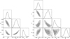 |
Fig. A.1 DESI-BAO+OHD contour plots of the cosmographic series up to j0 (left) and up to s0 (right). The best-fit parameters are indicated by black circles, whereas the 1σ (2σ) contours are shown as dark (light) grey areas. |
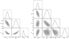 |
Fig. A.2 DESI-BAO+SN contour plots of the cosmographic series up to j0 (left) and up to s0 (right). Symbols and colours have the same meaning as in Fig. A.1 |
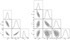 |
Fig. A.3 DESI-BAO+OHD+SN contour plots of the cosmographic series up to j0 (left) and up to s0 (right). Symbols and colours have the same meaning as in Fig. A.1. |
References
- Alfano, A. C., Cafaro, C., Capozziello, S., & Luongo, O. 2023, Phys. Dark Universe, 42, 101298 [NASA ADS] [CrossRef] [Google Scholar]
- Aviles, A., & Cervantes-Cota, J. L. 2011, Phys. Rev. D, 84, 089905 [NASA ADS] [CrossRef] [Google Scholar]
- Aviles, A., Gruber, C., Luongo, O., & Quevedo, H. 2012, Phys. Rev. D, 86, 123516 [CrossRef] [Google Scholar]
- Aviles, A., Bravetti, A., Capozziello, S., & Luongo, O. 2013a, Phys. Rev. D, 87, 064025 [NASA ADS] [CrossRef] [Google Scholar]
- Aviles, A., Bravetti, A., Capozziello, S., & Luongo, O. 2013b, Phys. Rev. D, 87, 044012 [NASA ADS] [CrossRef] [Google Scholar]
- Aviles, A., Bravetti, A., Capozziello, S., & Luongo, O. 2014, Phys. Rev. D, 90, 043531 [NASA ADS] [CrossRef] [Google Scholar]
- Bamba, K., Capozziello, S., Nojiri, S., & Odintsov, S. D. 2012, Astrophys. Space Sci., 342, 155 [NASA ADS] [CrossRef] [Google Scholar]
- Bargiacchi, G., Dainotti, M. G., & Capozziello, S. 2023, MNRAS, 525, 3104 [NASA ADS] [CrossRef] [Google Scholar]
- Borghi, N., Moresco, M., & Cimatti, A. 2022, ApJ, 928, L4 [NASA ADS] [CrossRef] [Google Scholar]
- Calzá, M., Casalino, A., Luongo, O., & Sebastiani, L. 2020, Eur. Phys. J. Plus, 135, 1 [CrossRef] [Google Scholar]
- Capozziello, S., Farooq, O., Luongo, O., & Ratra, B. 2014, Phys. Rev. D, 90, 044016 [NASA ADS] [CrossRef] [Google Scholar]
- Capozziello, S., Luongo, O., & Saridakis, E. N. 2015, Phys. Rev. D, 91, 124037 [CrossRef] [Google Scholar]
- Capozziello, S., D’Agostino, R., & Luongo, O. 2017, Gen. Relativity Grav., 49, 141 [NASA ADS] [CrossRef] [Google Scholar]
- Capozziello, S., D’Agostino, R., & Luongo, O. 2018a, MNRAS, 476, 3924 [NASA ADS] [CrossRef] [Google Scholar]
- Capozziello, S., D’Agostino, R., & Luongo, O. 2018b, JCAP, 2018, 008 [CrossRef] [Google Scholar]
- Capozziello, S., D’Agostino, R., & Luongo, O. 2019, Int. J. Mod. Phys. D, 28, 1930016 [NASA ADS] [CrossRef] [Google Scholar]
- Capozziello, S., D’Agostino, R., & Luongo, O. 2020, MNRAS, 494, 2576 [NASA ADS] [CrossRef] [Google Scholar]
- Capozziello, S., Dunsby, P. K. S., & Luongo, O. 2022, MNRAS, 509, 5399 [Google Scholar]
- Carloni, Y., Luongo, O., & Muccino, M. 2024, arXiv e-prints, [arXiv:2404.12068] [Google Scholar]
- Cattoën, C., & Visser, M. 2008, Phys. Rev. D, 78, 063501 [CrossRef] [Google Scholar]
- Colgáin, E. Ó., Dainotti, M. G., Capozziello, S., et al. 2024, arXiv e-prints, [arXiv:2404.08633] [Google Scholar]
- Copeland, E. J., Sami, M., & Tsujikawa, S. 2006, Int. J. Mod. Phys. D, 15, 1753 [NASA ADS] [CrossRef] [Google Scholar]
- de la Cruz-Dombriz, Á., Dunsby, P. K. S., Luongo, O., & Reverberi, L. 2016, JCAP, 2016, 042 [NASA ADS] [CrossRef] [Google Scholar]
- DESI Collaboration (Adame, A. G., et al.) 2024, arXiv e-prints, [arXiv:2404.03002] [Google Scholar]
- Di Valentino, E., Mena, O., Pan, S., et al. 2021, Class. Quant. Grav., 38, 153001 [NASA ADS] [CrossRef] [Google Scholar]
- Dunsby, P. K. S., & Luongo, O. 2016, Int. J. Geom. Methods Mod. Phys., 13, 1630002 [Google Scholar]
- Glanville, A., Howlett, C., & Davis, T. M. 2021, MNRAS, 503, 3510 [NASA ADS] [CrossRef] [Google Scholar]
- Gruber, C., & Luongo, O. 2014, Phys. Rev. D, 89, 103506 [NASA ADS] [CrossRef] [Google Scholar]
- Harrison, E. R. 1976, Nature, 260, 591 [NASA ADS] [CrossRef] [Google Scholar]
- Izzo, L., Luongo, O., & Capozziello, S. 2012, Mem. Soc. Astron. Ital. Suppl., 19, 37 [Google Scholar]
- Jiao, K., Borghi, N., Moresco, M., & Zhang, T.-J. 2023, ApJS, 265, 48 [NASA ADS] [CrossRef] [Google Scholar]
- Jimenez, R., & Loeb, A. 2002, ApJ, 573, 37 [NASA ADS] [CrossRef] [Google Scholar]
- Kunz, M. 2012, Comptes Rendus Phys., 13, 539 [NASA ADS] [CrossRef] [Google Scholar]
- Kunz, M., Trotta, R., & Parkinson, D. R. 2006, Phys. Rev. D, 74, 023503 [NASA ADS] [CrossRef] [Google Scholar]
- Landsberg, P. T., & Pathria, R. K. 1974, ApJ, 192, 577 [CrossRef] [Google Scholar]
- Luongo, O. 2011, Mod. Phys. Lett. A, 26, 1459 [NASA ADS] [CrossRef] [Google Scholar]
- Luongo, O. 2013, Mod. Phys. Lett. A, 28, 1350080 [NASA ADS] [CrossRef] [Google Scholar]
- Luongo, O., & Quevedo, H. 2014a, Int. J. Mod. Phys. D, 23, 1450012 [NASA ADS] [CrossRef] [Google Scholar]
- Luongo, O., & Quevedo, H. 2014b, Gen. Rel. Grav., 46, 1649 [NASA ADS] [CrossRef] [Google Scholar]
- Luongo, O., & Muccino, M. 2018, Phys. Rev. D, 98, 103520 [CrossRef] [Google Scholar]
- Luongo, O., & Muccino, M. 2021, MNRAS, 503, 4581 [NASA ADS] [CrossRef] [Google Scholar]
- Luongo, O., & Muccino, M. 2023, MNRAS, 518, 2247 [Google Scholar]
- Luongo, O., Pisani, G. B., & Troisi, A. 2016, Int. J. Mod. Phys. D, 26, 1750015 [Google Scholar]
- Montiel, A., Cabrera, J. I., & Hidalgo, J. C. 2021, MNRAS, 501, 3515 [Google Scholar]
- Moresco, M. 2015, MNRAS, 450, L16 [NASA ADS] [CrossRef] [Google Scholar]
- Moresco, M., Cimatti, A., Jimenez, R., et al. 2012, JCAP, 2012, 006 [CrossRef] [Google Scholar]
- Moresco, M., Pozzetti, L., Cimatti, A., et al. 2016, JCAP, 2016, 014 [CrossRef] [Google Scholar]
- Moresco, M., Amati, L., Amendola, L., et al. 2022, Living Rev. Relat., 25, 6 [CrossRef] [Google Scholar]
- Muccino, M., Luongo, O., & Jain, D. 2023, MNRAS, 523, 4938 [NASA ADS] [CrossRef] [Google Scholar]
- Perivolaropoulos, L., & Skara, F. 2022, New Astron. Rev., 95, 101659 [CrossRef] [Google Scholar]
- Planck Collaboration VI. 2020, A&A, 641, A6 [NASA ADS] [CrossRef] [EDP Sciences] [Google Scholar]
- Ratsimbazafy, A. L., Loubser, S. I., Crawford, S. M., et al. 2017, MNRAS, 467, 3239 [NASA ADS] [CrossRef] [Google Scholar]
- Riess, A. G., Rodney, S. A., Scolnic, D. M., et al. 2018, ApJ, 853, 126 [NASA ADS] [CrossRef] [Google Scholar]
- Sahni, V., & Starobinsky, A. 2006, Int. J. Mod. Phys. D, 15, 2105 [NASA ADS] [CrossRef] [Google Scholar]
- Scolnic, D. M., Jones, D. O., Rest, A., et al. 2018, ApJ, 859, 101 [NASA ADS] [CrossRef] [Google Scholar]
- Simon, J., Verde, L., & Jimenez, R. 2005, Phys. Rev. D, 71, 123001 [NASA ADS] [CrossRef] [Google Scholar]
- Stern, D., Jimenez, R., Verde, L., Kamionkowski, M., & Stanford, S. A. 2010, JCAP, 2010, 008 [Google Scholar]
- Sutherland, W. 2012, MNRAS, 426, 1280 [CrossRef] [Google Scholar]
- Tomasetti, E., Moresco, M., Borghi, N., et al. 2023, A&A, 679, A96 [NASA ADS] [CrossRef] [EDP Sciences] [Google Scholar]
- Tsujikawa, S. 2011, in Astrophysics and Space Science Library, 370, eds. S. Matarrese, M. Colpi, V. Gorini, & U. Moschella, 331 [NASA ADS] [CrossRef] [Google Scholar]
- Visser, M. 1997, Science, 276, 88 [NASA ADS] [CrossRef] [Google Scholar]
- Visser, M. 2005, Gen. Relat. Grav., 37, 1541 [CrossRef] [Google Scholar]
- Visser, M. 2015, Class. Quant. Grav., 32, 135007 [NASA ADS] [CrossRef] [Google Scholar]
- Wang, D. 2024, arXiv e-prints, [arXiv:2404.13833] [Google Scholar]
- Weinberg, S. 1972, Gravitation and Cosmology: Principles and Applications of the General Theory of Relativity [Google Scholar]
- Weinberg, S. 1989, Rev. Mod. Phys., 61, 1 [NASA ADS] [CrossRef] [Google Scholar]
- Zhang, C., Zhang, H., Yuan, S., et al. 2014, Res. Astron. Astrophys., 14, 1221 [CrossRef] [Google Scholar]
However, the DESI outcome represents another issue that increases the actual considerable conceptual and theoretical issues (Perivolaropoulos & Skara 2022) associated with the standard cosmological model, such as tensions (Di Valentino et al. 2021), fine-tuning, the coincidence problem, the cosmological constant problem (Luongo & Muccino 2018), and so on (Capozziello et al. 2019).
We arbitrarily neglect in our analyses the possibility of working out auxiliary variables, as proposed in Aviles et al. (2012), Visser (2015), Visser (2005) and Cattoën & Visser (2008) or alternatives to Taylor expansions as shown in Gruber & Luongo (2014) and Capozziello et al. (2020).
The model fully degenerates with the dark fluid, that conversely to the ΛCDM scenario provides an evolving equation of state, albeit with constant pressure (see e.g. Luongo & Quevedo 2014a; Luongo & Quevedo 2014b; Luongo & Muccino 2018).
All Tables
All Figures
|
Fig. A.1 DESI-BAO+OHD contour plots of the cosmographic series up to j0 (left) and up to s0 (right). The best-fit parameters are indicated by black circles, whereas the 1σ (2σ) contours are shown as dark (light) grey areas. |
| In the text | |
|
Fig. A.2 DESI-BAO+SN contour plots of the cosmographic series up to j0 (left) and up to s0 (right). Symbols and colours have the same meaning as in Fig. A.1 |
| In the text | |
|
Fig. A.3 DESI-BAO+OHD+SN contour plots of the cosmographic series up to j0 (left) and up to s0 (right). Symbols and colours have the same meaning as in Fig. A.1. |
| In the text | |
Current usage metrics show cumulative count of Article Views (full-text article views including HTML views, PDF and ePub downloads, according to the available data) and Abstracts Views on Vision4Press platform.
Data correspond to usage on the plateform after 2015. The current usage metrics is available 48-96 hours after online publication and is updated daily on week days.
Initial download of the metrics may take a while.