| Issue |
A&A
Volume 689, September 2024
|
|
|---|---|---|
| Article Number | A215 | |
| Number of page(s) | 11 | |
| Section | Cosmology (including clusters of galaxies) | |
| DOI | https://doi.org/10.1051/0004-6361/202450342 | |
| Published online | 16 September 2024 | |
Testing cosmic anisotropy with Padé approximations and the latest Pantheon+ sample
1
School of Astronomy and Space Science, Nanjing University, Nanjing, 210093
China
e-mail: This email address is being protected from spambots. You need JavaScript enabled to view it.
2
School of Engineering, Dali University, Dali, 671003
China
3
Research Center for Astronomical Computing, Zhejiang Lab, Hangzhou, 311100
China
4
Key Laboratory of Modern Astronomy and Astrophysics (Nanjing University), Ministry of Education, Nanjing, 210093
China
Received:
12
April
2024
Accepted:
20
June
2024
Abstract
Cosmography can be used to constrain the kinematics of the Universe in a model-independent way. In this work, we attempt to combine the Padé approximations with the latest Pantheon+ sample to test the cosmological principle. Based on the Padé approximations, we first applied cosmographic constraints to different-order polynomials including third-order (Padé(2, 1)), fourth-order (Padé(2, 2)), and fifth-order (Padé(3, 2)) ones. The statistical analyses show that the Padé(2, 1) polynomial has the best performance. Its best fits are H0 = 72.53 ± 0.28 km s−1 Mpc−1, q0 = −0.35−0.07+0.08, and j0 = 0.43−0.56+0.38. By further fixing j0 = 1.00, it can be found that the Padé(2, 1) polynomial can describe the Pantheon+ sample better than the regular Padé(2, 1) polynomial and the usual cosmological models (including the ΛCDM, wCDM, CPL, and Rh = ct models). Based on the Padé(2, 1) (j0 = 1) polynomial and the hemisphere comparison method, we tested the cosmological principle and found the preferred directions of cosmic anisotropy, such as (l, b) = (304.6°−37.4+51.4, −18.7°−20.3+14.7) and (311.1°−8.4+17.4, −17.53°−7.7+7.8) for q0 and H0, respectively. These two directions are consistent with each other at a 1σ confidence level, but the corresponding results of statistical isotropy analyses including isotropy and isotropy with real positions are quite different. The statistical significance of H0 is stronger than that of q0; that is, 4.75σ and 4.39σ for isotropy and isotropy with real positions, respectively. Reanalysis with fixed q0 = −0.55 (corresponds to Ωm = 0.30) gives similar results. Overall, our model-independent results provide clear indications of a possible cosmic anisotropy, which must be taken seriously. Further testing is needed to better understand this signal.
Key words: supernovae: general / cosmological parameters / cosmology: theory
Corresponding author; This email address is being protected from spambots. You need JavaScript enabled to view it. .
© The Authors 2024
 Open Access article, published by EDP Sciences, under the terms of the Creative Commons Attribution License (https://creativecommons.org/licenses/by/4.0), which permits unrestricted use, distribution, and reproduction in any medium, provided the original work is properly cited.
This article is published in open access under the Subscribe to Open model. This email address is being protected from spambots. You need JavaScript enabled to view it. to support open access publication.
1. Introduction
Cosmography has been widely used in cosmological data processing to restrict the state of the kinematics of our Universe in a model-independent way (Visser 2015; Dunsby & Luongo 2016; Capozziello et al. 2018a, 2019a,b; Lusso et al. 2019; Bargiacchi et al. 2021). It relies only on the assumption of a homogeneous and isotropic Universe described by the Friedman-Lemaitre-Robertson-Walker (FLRW) metric (Weinberg 1972). Its methodology is essentially based on expanding the measurable cosmological quantity into the Taylor series around the present time. In this framework, the evolution of the Universe can be described by some cosmographic parameters, such as the Hubble parameter (H), deceleration (q), jerk (j), snap (s), and lerk (l) parameters. The corresponding definitions of them can be expressed as follows:
 (1)
(1)
Various methods have been proposed in the literature. The first proposed method is z-redshift (Caldwell & Kamionkowski 2004; Riess et al. 2004; Visser 2004), which estimated the cosmic evolution as z ∼ 0 well, but which failed at high redshifts (Chiba et al. 1998; Riess et al. 2004; Visser 2004; Wang et al. 2009; Vitagliano et al. 2010). The main reason is that the data are far from the limits of Taylor expansions. In cosmography, this is called the convergence problem. Focusing on this issue, many improved methods have been proposed to solve this problem, such as y-redshift (Chevallier & Polarski 2001; Linder 2003; Vitagliano et al. 2010), E(y) (Rezaei et al. 2020), log(1 + z) (Risaliti & Lusso 2019; Yang et al. 2020), log(1 + z) + kij (Bargiacchi et al. 2021), Padé approximations (Gruber & Luongo 2014; Wei et al. 2014; Capozziello et al. 2020), and Chebyshev approximations (Capozziello et al. 2018a). In theory, the improved methods can effectively avoid the convergence problem. Analyses combined with cosmic observations show that things are not simple (Zhang et al. 2017; Hu et al. 2020; Rezaei et al. 2020; Hu & Wang 2022a). Zhang et al. (2017) found that the y-redshift produces larger variances beyond the second-order expansion from the analyses of the joint light curve analysis sample (JLA; Betoule et al. 2014). A similar result was also found by Rezaei et al. (2020) using a composite sample that included type Ia supernovae (SNe Ia), quasars, and gamma-ray bursts (GRBs). They attempted to recast E(z) as a function of y = z/(1 + z) and adopted the new series expansion of the E(y) function to compare dark energy models. For the convergence problem of the cosmographic method, there are still many details that need to be further studied.
Many works have compared the strengths of the different cosmographic techniques by utilizing different observational data (Capozziello et al. 2018a, 2020; Hu & Wang 2022a; Pourojaghi et al. 2022). Utilizing the Akaike information criterion (AIC; Akaike 1974) and the Bayesian information criterion (BIC; Schwarz 1978), Capozziello et al. (2020) critically compared the auxiliary variables with the rational approximations, including y1 = 1 − a, y2 = arctan(a−1 − 1), and the Padé approximations. They found that even though y2 overcomes the issues of y1, the performance of Padé approximations is better than that of the auxiliary variables y1 = 1 − a and y2 = arctan(a−1 − 1). Meanwhile, they also made Monte Carlo analyses, combining the Pantheon sample, H(z), and shift parameter measurements, and concluded that the Padé(2, 1) polynomial is statistically the optimal approach to explain low- and high-redshift observations. Utilizing the Pantheon sample (Scolnic et al. 2018) and 31 long GRBs (Wang et al. 2022), Hu & Wang (2022a) made a systematic comparison among the commonly used cosmographic expansions (including z-redshift, y-redshift, E(y), log(1 + z), log(1 + z)+kij, and Padé approximations) with different expansion orders. They found that the expansion order can significantly affect the results, especially the y-redshift method. The Padé(2, 1) polynomial is suitable for both low- and high- redshift cases. The Padé(2, 2) polynomial performs well in the high-redshift case. According to the statistical results, they conclude that it is important to choose a suitable expansion method and order based on the sample used. From previous comparative research, it has been found that the Padé approximations perform better than the traditional Taylor series.
Recently, the latest sample of SNe Ia (Pantheon+) was released by the SH0ES collaboration (Brout et al. 2022; Scolnic et al. 2022). It is the updated version of the Pantheon sample, and covers the redshift range of (0.001, 2.26). This latest sample has been widely used for cosmological applications, such as cosmological constraints (Cao & Ratra 2023; Dainotti et al. 2023b; Favale et al. 2023; Pastén & Cárdenas 2023; Qi et al. 2023; Scolnic et al. 2023), non-Gaussian likelihoods (Dainotti et al. 2023a; Lovick et al. 2023), absolute magnitudes (Chen et al. 2024; Perivolaropoulos & Skara 2023; Liu et al. 2024), modified gravity (dos Santos 2023; Kumar et al. 2023; Valdez et al. 2023), dynamical dark energy (Tutusaus et al. 2023; Van Raamsdonk & Waddell 2024), the running vacuum in the Universe (Solà Peracaula et al. 2023; Yershov 2023; Gómez-Valent et al. 2024), Hubble tension (Jia et al. 2023; Simon 2024; Yadav 2023; Adil et al. 2024; Jia et al. 2024), σ8 tension (Poulin et al. 2023), the cosmological principle (Mc Conville & Colgáin 2023; Perivolaropoulos 2023; Tang et al. 2023; Bengaly et al. 2024; Hu et al. 2024), and so on. The cosmological principle is the basic assumption of cosmology, which requires that the Universe is statistically isotropic and uniform on a sufficiently large scale. However, much research suggests that the Universe may be inhomogeneous and anisotropic, including the fine-structure constant (Milaković et al. 2023), the direct measurement of the Hubble parameter (Koksbang 2021), and source counts (Singal 2023). In recent years, SNe Ia have been widely employed to test the cosmological principle (Sun & Wang 2018; Colin et al. 2019; Kalbouneh et al. 2023; Mc Conville & Colgáin 2023; Perivolaropoulos 2023; Tang et al. 2023; Hu et al. 2024). Tang et al. (2023) fit the full Pantheon+ data with the dipole-modulated ΛCDM model and found that the dipole appears at a 2σ confidence level if zc ≤ 0.1. Perivolaropoulos (2023) used the hemisphere comparison (HC) method to test the isotropy of the SNe Ia absolute magnitudes of the Pantheon+ and SH0ES samples in various redshift or distance bins. They found sharp changes in the level of anisotropy occurring at distances less than 40 Mpc. Meanwhile, Mc Conville & Colgáin (2023) also employed the Pantheon+ sample to analyse the anisotropic distance ladder and found a larger H0 near by the cosmic microwave background (CMB) dipole direction. They point out that the cosmic anisotropy may be due to a breakdown in the cosmological principle (Krishnan et al. 2022), or mundanely due to a statistical fluctuation in a small sample of SNe in Cepheid host galaxies. Employing the Pantheon+ sample, Hu et al. (2024) propose a new method named the region-fitting method to map the all-sky distribution of cosmological parameters to examine the cosmological principle. They found a local matter underdensity region ( ,
,  ) and a preferred direction of cosmic anisotropy (
 ,
,  ) in galactic coordinates. Based on investigating the correlation between the degree of cosmic anisotropy and the redshift, they also propose that H0 evolution (Krishnan et al. 2020; Millon et al. 2020; Wong et al. 2020; Dainotti et al. 2021; Hu & Wang 2022b; Jia et al. 2023; Malekjani et al. 2024) might be associated with the violation of the cosmological principle. At present, the anisotropy of the accelerating expansion of the Universe is still unresolved (Migkas et al. 2021; Akarsu et al. 2022; Abdalla et al. 2022; Horstmann et al. 2022; Perivolaropoulos & Skara 2022; Akarsu et al. 2023; Bhanja et al. 2023; Kumar Aluri et al. 2023; Kalbouneh et al. 2024; Migkas 2024; Nyagisera et al. 2024; Patel & Desmond 2024; Yadav et al. 2024). Most of the above research into the cosmological principle is based on the ΛCDM model or other extended models. Until now, no research has considered using the Padé approximation to probe the cosmological principle.
In this paper, we have utilized the latest Pantheon+ sample and the Padé approximation for cosmological applications including cosmographic constraints, model comparison, and the cosmological principle. Firstly, we gave the cosmographic constraints, and tried to find out the suitable expansion order of the Pantheon+ sample. After that, we critically compared the Padé approximation with common cosmological models, such as the flat ΛCDM model, non-flat ΛCDM model, wCDM model, Chevallies-Polarski-Linder (CPL) model (Chevallier & Polarski 2001; Linder 2003), and Rh = ct model (Melia & Shevchuk 2012). In addition, we mapped the anisotropy level (AL) in the galactic coordinate system, utilizing the Pantheon+ sample based on the Padé approximation and the HC method. For strict consideration, the corresponding statistical isotropy analyses were done. The outline of this paper is as follows. In Section 2, we describe the observational data and fitting method. Theoretical models used in this article are introduced in Section 3. In Section 4, we describe the HC method used to probe the preferred direction of cosmic anisotropy. Afterward, we present and discuss the main results in Section 5. Finally, a brief summary is given in Section 6.
2. Observational data and fitting method
2.1. Pantheon+ sample
The Pantheon+ sample is the latest SNe Ia dataset (Brout et al. 2022; Scolnic et al. 2022). It consists of 1701 SNe Ia light curves observed from 1550 distinct SNe, and covers a redshift range of (0.001, 2.26). In Fig. 1, we give some basic information including the cumulative distribution of redshift (left panel) and the location distribution in the galactic coordinate system (right panel). From the left panel of Fig. 1, it is easy to find that the redshift of nearly half of the observations (44%) is below 0.10, and for most of the observations (95%) it is below 0.70. From the right panel of Fig. 1, we can find that the belt-like structure still plays the most important role in the Pantheon+ sample although the number of new added SNe is around 700. Combining the redshift information, it can be found that the distribution of SNe whose redshifts are smaller than 0.10 is relatively homogeneous. However, the distribution of higher-redshift SNe is relatively concentrated, because they are mainly obtained from some high-redshift surveys, such as the Sloan Digital Sky Survey (SDSS; Sako et al. 2018), the Panoramic Survey Telescope & Rapid Response System Medium Deep Survey (PS1MD; Scolnic et al. 2018), the SuperNova Legacy Survey (SNLS; Betoule et al. 2014), and so on. In a nutshell, the SNe distribution of Pantheon+ sample is still inhomogeneous. In addition, it is noted that SNe Ia have a nearly uniform intrinsic luminosity with an absolute magnitude of M ∼ −19.5 (Carroll 2001), which makes them a well-established class of standard candles. The difficulty in cosmological applications lies in the identification of the absolute magnitude, M, due to different sources of systematic and statistical uncertainties. In this paper, systematic (Csys) and statistical (Cstat) covariance matrices were considered. The datasets used, the distance modulus, μob, and the total covariance matric, Cstat + sys, were provided by Brout et al. (2022) and publicly available1. The observational distance modulus was calibrated by the second rung of the distance ladder using Cepheids measuring the SNe Ia absolute magnitude as MB = −19.25 ± 0.01 (Brout et al. 2022; Riess et al. 2022; Bousis & Perivolaropoulos 2024).
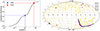 |
Fig. 1. Basic information about the Pantheon+ sample. The left panel shows the cumulative redshift distribution. The right panel shows the location of different redshift SNe in the galactic coordinate system. |
2.2. Fitting method
The best fits of the cosmological parameters were derived by minimizing the chi-square (χ2),
 (2)
(2)
where μobs is the observational distance modulus and μth is the theoretical distance modulus, which can be obtained from the following formula:
 (3)
(3)
Here, zi is the peculiar-velocity-corrected CMB-frame redshift of each SN (Carr et al. 2022), Pi represents the parameters to be fitted, M is the absolute magnitude, m is the apparent magnitude of the source, and dL is the luminosity distance. For the calculation of dL, we needed to fix a cosmological model or expansion method. Here, we briefly introduce how to obtain dL based on the Padé approximations and some common cosmological models, including Padé(2, 1), Padé(2, 2), Padé(3, 2), the flat ΛCDM model, the non-flat ΛCDM model, the wCDM model, the CPL model, and the Rh = ct model.
3. Theoretical models
Padé approximations. The Padé approximations (Steven & Harold 1992) were built up from the standard Taylor definition and can be used to lower divergences at z≥ 1. They often give a better approximation of the function than truncating its Taylor series, and they may still work where the Taylor series does not converge (Wei et al. 2014). Due to their excellent convergence properties, the Padé polynomials have been considered at high redshifts in cosmography (Gruber & Luongo 2014; Demianski et al. 2017; Capozziello et al. 2018b, 2020). The Taylor expansion of a generic function, f(z), can be described by a given function,  , where ci = fi(0)/i!, which is approximated by means of an (n, m) Padé approximation by the radio polynomial (Capozziello et al. 2020)
 (4)
(4)
there is a total (n + m + 1) number of independent coefficients. In the numerator, we have n + 1 independent coefficients, whereas in the denominator there is m. Since, by construction, b0 = 1 is required, we have
 (5)
(5)
The coefficients, bi, in Eq. (4) were thus determined by solving the following homogeneous system of linear equations (Litvinov 1993):
 (6)
(6)
which is valid for k = 1, …, m. All of the coefficients, ai, in Eq. (4) can be computed using the formula
 (7)
(7)
In terms of the investigations of Capozziello et al. (2020) into the Padé approximation, we finally chose to use the Padé(2, 1), Padé(2, 2), and Padé(3, 2) polynomials to represent the third-order, fourth-order, and fifth-order polynomials, respectively. More detailed information about the selections of the specific polynomials can be found in Capozziello et al. (2020). The corresponding luminosity distances are given as follows.
(1) Padé(2, 1) polynomial of the luminosity distance:
![Mathematical equation: $$ \begin{aligned} d_{\rm L} = \frac{c}{H_{0}}[ \frac{z(6(-1+q_{0})+(-5-2j_{0}+q_{0}(8+3q_{0}))z)}{-2(3+z+j_{0}z)+2q_{0}(3+z+3q_{0}z)}]. \end{aligned} $$](/articles/aa/full_html/2024/09/aa50342-24/aa50342-24-eq19.gif) (8)
(8)
(2) Padé(2, 2) polynomial of the luminosity distance:
![Mathematical equation: $$ \begin{aligned} d_{\rm L}&= \frac{c}{H_0}[6z(10 + 9 z - 6 q_0^3 z + s_0 z - 2 q_0^2 (3 + 7 z) \nonumber \\&\quad - q_0 (16 + 19 z) + j_0 (4 + (9 + 6 q_0) z))\Big /(60 + 24 z \nonumber \\&\quad + 6 s_0 z - 2 z^2 + 4 j_0^2 z^2 - 9 q_0^4 z^2 - 3 s_0 z^2 \nonumber \\&\quad +6 q_0^3 z (-9 + 4 z) + q_0^2 (-36 - 114 z + 19 z^2) \nonumber \\&\quad + j_0 (24 + 6 (7 + 8 q_0) z + (-7 - 23 q_0 + 6 q_0^2) z^2) \nonumber \\&\quad + q_0 (-96 - 36 z + (4 + 3 s_0) z^2))]. \end{aligned} $$](/articles/aa/full_html/2024/09/aa50342-24/aa50342-24-eq20.gif) (9)
(9)
(3) Padé(3, 2) polynomial of the luminosity distance:
![Mathematical equation: $$ \begin{aligned} d_{\rm L}&=\frac{c}{H_0}[z (-120 - 180 s_0 - 156 z - 36 l_0 z - 426 s_0 z \nonumber \\&\quad - 40 z^2 + 80 j_0^3 z^2 - 30 l_0 z^2 - 135 q_0^6 z^2 - 210 s_0 z^2 \nonumber \\&\quad + 15 s_0^2 z^2 - 270 q_0^5 z (3 + 4 z) + 9 q_0^4 (-60 + 50 z + 63 z^2) \nonumber \\&\quad + 2 q_0^3 (720 + 1767 z + 887 z^2) + 3 j_0^2 (80 + 20 (13 + 2 q_0) z \nonumber \\&\quad + (177 + 40 q_0 - 60 q_0^2) z^2) + 6 q_0^2 (190 + 5 (67 + 9 s_0) z \nonumber \\&\quad + (125 + 3 l_0 + 58 s_0) z^2) -6 q_0 (s_0 (-30 + 4 z + 17 z^2) \nonumber \\&\quad - 2 (20 + (31 + 3 l_0) z + (9 + 4 l_0) z^2)) + 6 j_0 (-70 \nonumber \\&\quad + (-127 + 10 s_0) z + 45 q_0^4 z^2 + (-47 - 2 l_0 + 13 s_0) z^2 \nonumber \\&\quad + 5 q_0^3 z (30 + 41 z) - 3 q_0^2 (-20 + 75 z + 69 z^2) \nonumber \\&\quad + 2 q_0 (-115 - 274 z + (-136 + 5 s_0) z^2)))]\Big /[3(-40 \nonumber \\&\quad - 60 s_0 - 32 z - 12 l_0 z - 112 s_0 z - 4 z^2 + 40 j_0^3 z^2 - 4 l_0 z^2 \nonumber \\&\quad - 135 q_0^6 z^2 - 24 s_0 z^2 + 5 s_0^2 z^2 - 30 q_0^5 z (12 + 5 z) \nonumber \\&\quad + 3 q_0^4 (-60 + 160 z + 71 z^2) +j_0^2 (80 + 20 (11 + 4 q_0) z \nonumber \\&\quad + (57 + 20 q_0 - 40 q_0^2) z^2) + 6 q_0^3 (80 + 188 z + (44 \nonumber \\&\quad + 5 s_0) z^2) + 2 q_0^2 (190 + 20 (13 + 3 s_0) z + (46 + 6 l_0 \nonumber \\&\quad + 21 s_0) z^2)+4 q_0 (20 + (16 + 3 l_0) z + (2 + l_0) z^2 \nonumber \\&\quad + s_0 (15 - 17 z - 9 z^2))+2 j_0 (-70 + 2 (-46 + 5 s_0) z \nonumber \\&\quad + 90 q_0^4 z^2 + (-16 - 2 l_0 + 3 s_0) z^2 + 15 q_0^3 z (12 + 5 z) \nonumber \\&\quad + q_0^2 (60 - 370 z - 141 z^2) + 2 q_0 (-115 - 234 z \nonumber \\&\quad + 2 (-26 + 5 s_0) z^2)))], \end{aligned} $$](/articles/aa/full_html/2024/09/aa50342-24/aa50342-24-eq21.gif) (10)
(10)
where c is the speed of light, and H0, q0, j0, s0, and l0 represent current values.
Flat ΛCDM model. Considering the flat ΛCDM model, the corresponding luminosity distance, dL, can be calculated from (Hu et al. 2021)
 (11)
(11)
where Ωm is the matter density and ΩΛ is the dark energy density.
Non-flat ΛCDM model. For the nonflat ΛCDM model, the corresponding luminosity distance, dL, should be written as (Hu et al. 2021)
![Mathematical equation: $$ \begin{aligned} d_{\rm L} = {\left\{ \begin{array}{ll} \frac{c(1+z)}{H_{0}}(-\Omega _{\rm k})^{-\frac{1}{2}} \sin {[(-\Omega _{\rm k})^{\frac{1}{2}} \int _{0}^{z} \frac{dz^\prime }{E(z^\prime )}]},&\Omega _{\rm k} < 0, \\ \frac{c(1+z)}{H_{0}} \int _{0}^{z} \frac{dz^\prime }{E(z^\prime )},&\Omega _{\rm k} = 0,\\ \frac{c(1+z)}{H_{0}}\Omega _{\rm k}^{-\frac{1}{2}} \sinh {[\Omega _{\rm k}^{\frac{1}{2}} \int _{0}^{z} \frac{dz^\prime }{E(z^\prime )}]},&\Omega _{\rm k} > 0, \end{array}\right.} \end{aligned} $$](/articles/aa/full_html/2024/09/aa50342-24/aa50342-24-eq23.gif) (12)
(12)
 (13)
(13)
here, Ωk is the spatial curvature.
wCDM model. For the wCDM model, the corresponding luminosity distance, dL, can be written as (Li et al. 2023)
 (14)
(14)
where w0 represents the constant equation of state (EoS). When w0 ≃ −1, this model regresses to the flat ΛCDM model.
CPL model. Rewriting Eq. (14), we can obtain the corresponding expression of luminosity distance for the CPL model (Chevallier & Polarski 2001; Linder 2003):
 (15)
(15)
In the CPL model, dark energy evolves with redshift as a parameterized EoS, w = w0 + waz/(1 + z).
Rh = ct model. For the Rh = ct model (Melia & Shevchuk 2012), the corresponding luminosity distance is as follows:
 (16)
(16)
where Rh(t0) is the current gravitational horizon, which can also be represented by c/H0.
Combining Eqs. (2), (3), and the expressions of luminosity distance, we can produce the corresponding constraints for the different expansion methods or cosmological models. The comparison results of different constraints are obtained by utilizing the Akaike information criterion (AIC; Schwarz 1978) and the Bayesian information criterion (BIC; Akaike 1974), which are the last set of techniques that can be employed for model comparison based on information theory. The corresponding definitions read as follows:
 (17)
(17)
 (18)
(18)
where n is the number of free parameters, N is the total number of data points, and ℒ is the maximum value of the likelihood function. The values of ℒ are derived from the following formula:
 (19)
(19)
where  is the value of χ2 calculated with the best-fitting results. The model that has lower values of AIC and BIC will be the suitable model for the employed dataset. Moreover, we also calculated the differences between ΔAIC and ΔBIC with respect to the corresponding flat ΛCDM values to measure the amount of information lost by adding extra parameters in the statistical fitting. Negative values of ΔAIC and ΔBIC suggest that the model under investigation performs better than the reference model. For positive values of ΔAIC and ΔBIC, we adopted the judgment criteria from the literature (Capozziello et al. 2020; Hu & Wang 2022a):
-
Δ AIC(BIC) ∈ [0,2] indicates weak evidence in favor of the reference model, leaving the question of which model is the most suitable open;
-
Δ AIC(BIC) ∈ [2,6] indicates mild evidence against the given model with respect to the reference paradigm; and
-
Δ AIC(BIC) > [0,2] indicates strong evidence against the given model, which should be rejected.
4. Hemisphere comparison method
The HC method proposed by Schwarz & Weinhorst (2007) has been widely used in the investigation of cosmic anisotropy, such as the anisotropy of cosmic expansion (Deng & Wei 2018a; Zhao & Xia 2022), the acceleration scale of modified Newtonian dynamics (Zhou et al. 2017; Chang et al. 2018), and the temperature anisotropy of the CMB (Hansen et al. 2004; Bennett et al. 2013; Ghosh et al. 2016; Ferreira 2021). Firstly, we briefly introduce this method. Its goal is to identify the direction, which corresponds to the axis of maximal asymmetry from the dataset, by comparing the accelerating expansion rate (q0). In the Padé approximations, it is convenient to employ H0 to replace the accelerating expansion rate, considering the relationship between the deceleration parameter, q0, and H0. The most important step is to generate random directions,  (l, b), to divide the SNe dataset into two subsamples (defined as “up” and “down”), where l ∈ (0°, 360° ) and b ∈ ( − 90°, 90° ) are the longitude and latitude in the galactic coordinate system, respectively. According to “up” and “down” subsamples, the corresponding best-fits of cosmological parameters are obtained by employing the Markov Chain Monte Carlo (MCMC) method. The AL made up of q0, u and q0, d can be used to describe the degree of deviation from isotropy. Its values can be derived from
 (20)
(20)
where q0, u and q0, d are the best fits of the “up” and “down” subsamples, respectively. These two subsamples are separated from the full SNe sample by a random direction,  . The 1σ uncertainty σAL is
 (21)
(21)
where  and
and  are the 1σ errors corresponding to
  and
and  . During the calculation, we repeated 10 000 random directions,
  . We note that if one prefers to employ other parameters (for example, H0) to find the preferred directions of cosmic anisotropy, it is convenient to replace the parameter q0 in Eqs. (20) and (21).
In order to examine whether the discrepancy degree of the cosmological parameters from the Pantheon+ sample is consistent with statistical isotropy, we carried out statistical isotropic analyses. To achieve this, we spread the original dataset evenly across the sky. After that, we were able to obtain ALmax for the isotropic dataset. Meanwhile, an additional isotropic analysis was also considered. We preserved the spatial inhomogeneity of the real sample and then randomly distributed the real dataset, which randomly redistributed the distance moduli and redshift combination to real-data positions (RPs) only. Given the limitations of computing time, we repeated this 1000 times; this produced acceptable statistics. For convenience, we refer to these two approaches as isotropy analysis and isotropy RP analysis.
5. Results and discussion
5.1. Cosmographic constraints
We first gave the cosmographic constraints of the Pantheon+ sample by utilizing the Padé approximations, including the Padé(2, 1), Padé(2, 2), and Padé(3, 2) polynomials. The final contours are shown in Fig. 2, and the detailed results are displayed in Table 1. Overall, there are tight constraints for all parameters, except for the Padé(3, 2) polynomial. For the Padé(2, 1) polynomial, the results are H0 = 72.53 ± 0.28 km/s/Mpc, q0 = −0.35 , and j0 = 0.43
 . For the Padé(2, 2) polynomial, the results are H0 = 72.48
 km/s/Mpc, q0 = −0.33
 , j0 = 0.13
 , and s0 = −0.56
 . For the Padé(3, 2) polynomial, the Pantheon+ sample could not produce a tight constraint for all the parameters (H0, q0, j0, s0, l0). To minimize risk, we only constrained the first two parameters (q0 and j0), while the other parameters were marginalized in a large range (0 < s0, l0 < 20) (Zhang et al. 2017; Hu & Wang 2022a). The final constraints are H0 = 72.33
 km/s/Mpc, q0 = −0.22
 , and j0 = −1.58
 . In the flat ΛCDM model, q0 = 3Ωm/2 − 1 and j0 = 1 are expected. We can find that all q0 and j0 results are consistent with the ΛCDM model, with Ωm = 0.3 within a 2σ level. For H0 constraints, they are in line with that from the SH0ES collaboration. The corresponding statistical information is shown in Table 2. Since the Padé(3, 2) polynomial could not constrain all free parameters well, it should not be considered. The statistical results show that the Pantheon+ sample prefers the Padé(2, 1) polynomial in the Padé approximations. After that, we also gave the constraints of H0 and q0, employing the Padé(2, 1) polynomial and fixing j0 = 1.0; that is, H0 = 72.74±0.22 km/s/Mpc and q0 = −0.43±0.03. For convenience, this is referred to as Padé(2, 1)(j0 = 1). It is worth noting that although the χ2 value increases slightly, the values of AIC and BIC decrease significantly. This indicates that the Padé(2, 1)(j0 = 1) polynomial is more suitable for the Pantheon+ sample than the Padé(2, 1) polynomial.
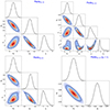 |
Fig. 2. Confidence contours (1σ and 2σ) and marginalized likelihood distributions for the parameter space (H0, q0, j0, and s0) from the Pantheon+ sample utilizing the Padé approximations including Padé(2, 1), Padé(2, 2), Padé(3, 2), and Padé(2, 1)(j0 = 1) polynomials. |
Best-fitting results at the 68 percent confidence level using the Pantheon+ sample under different expansion methods and cosmological models.
In addition, we also constrained the cosmological parameters, combining the Pantheon+ sample with the usual cosmological models, such as the flat ΛCDM, non-flat ΛCDM, wCDM, CPL, and Rh = ct models. The corresponding confidence contours are shown in Figs. A.1 (flat and non-flat ΛCDM models), A.2 (wCDM and CPL models), and A.3 (Rh = ct model). For the flat and non-flat ΛCDM models, the constraints are (H0 = 72.84±0.23 km/s/Mpc, Ωm = 0.36±0.02) and (H0 = 72.53 km/s/Mpc, Ωm = 0.26
 , ΩΛ = 0.48±0.08), respectively. The value of H0 is larger than that derived from H(z) data (Yu et al. 2018). For the wCDM model, the results are H0 = 72.51±0.27 km/s/Mpc, Ωm = 0.21
 , and w0 = −0.72
 . The results of the CPL model are H0 = 71.95
 km/s/Mpc, Ωm = 0.48
 , w0 = −0.52
 , and wa = −7.6
 . The result, H0 = 70.63±0.12 km/s/Mpc, was obtained using the Rh = ct model. Finally, we made a comparison investigation between the Padé approximations and the usual cosmological models in terms of the AIC and BIC methods. The detailed information is shown in Table 2. From the statistical information, we find that the Padé(2, 1)(j0 = 1) polynomials perform better than the usual cosmological models. The smallest values for ΔAIC and ΔBIC were obtained by the Padé(2, 1)(j0 = 1) polynomials; that is, ΔAIC = −2.7 and ΔBIC = −2.7. In addition, there is a negative value of ΔAIC but a positive value of ΔBIC, such as the non-flat ΛCDM model, the wCDM model, the CPL model, and Padé(2, 1)(j0 = 1) polynomials. Overall, the Padé(2, 1)(j0 = 1) polynomial can describe the Pantheon+ sample well.
Statistical results with respect to the reference flat ΛCDM model by utilizing the AIC and BIC statistical criteria.
5.2. Cosmic anisotropy
Based on the comparison analyses, we decided to combine the Padé(2, 1)(j0 = 1) polynomials with the HC method to find the preferred direction of cosmic anisotropy. Therefore, there exist two free parameters, q0 and H0. Previous work usually fixed the redundant parameters, leaving only one free parameter. Here, we chose to fit q0 and H0 simultaneously for the different SNe subsamples that were obtained by the random directions,  . Utilizing Eq. (20), we mapped the corresponding AL(l, b) distributions of q0 and H0 in the galactic coordinate system, as is shown in Fig. 3. From the AL distribution of q0 (upper panel), we find that there is a maximum value of AL, ALmax(q0) = 0.34, in the direction of (l, b) = (304.6
 , −18.7
 ). The corresponding 1σ error of AL was derived from Eq. (21) and used to plot the 1σ region; that is, σALmax = 0.08. For the parameter H0, we find that ALmax(H0) = 0.028, σALmax = 0.004, and (l, b) = (311.1
 , −17.53
 ), as is shown in the lower panel of Fig. 3. It is easy to cover that these two preferred directions are consistent with each other. However, ALmax and the corresponding σALmax values of q0 are larger than those of H0. In other words, the investigation of H0 gives a tighter constraint for the anisotropic direction, but its anisotropic degree is weaker than that given by the q0 investigation. This means that these two parameters might have different sensitivities to the cosmic anisotropy. According to the values of ALmax and σALmax, we plotted the probability density distributions of ALmax, as is shown in Fig. 4. This suggests that the results of Fig. 3 are a significant departure from isotropy (AL = 0).
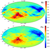 |
Fig. 3. Pseudo-color map of AL in the galactic coordinate system utilizing the HC method. The upper and lower panels show the results of q0 and H0, respectively. The blue star and line mark the direction of the largest AL and the corresponding 1σ range in the sky. The corresponding directions and 1σ areas are parameterized as ALmax,q0 (304.6 |


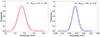 |
Fig. 4. Probability density distribution of the AL. The left and right panels are plotted by using ALmax(q0) = 0.34 ± 0.08 and ALmax(H0) = 0.028 ± 0.004), respectively. |
The statistical isotropic analyses including the isotropy and isotropy RP can be described well by Gaussian functions, as is shown in Fig. 5. For the isotropy analyses, the statistical significance of the real data is 1.72σ and 4.75σ for q0 and H0, respectively. The statistical significance of the real data derived from the isotropy RP analyses is 1.78σ for q0 and 4.39σ for H0. From the statistical results, we can find that the statistical significance of H0 is more obvious than that of q0. This might be caused by the sensitivity differences of parameters on the cosmic anisotropy. The isotropy analyses give more obvious statistical significance than that given by the isotropy RP analyses, especially the H0 investigations. This means that the spatial inhomogeneity can provide an additional contribution to the cosmic anisotropy. In addition, we also considered fixing q0 = −0.55, which corresponds to Ωm = 0.30, to make reanalyses. The corresponding results are shown in Figs. 6, 7, and 8. From the AL distribution, as is shown in Fig. 6, we obtained that ALmax(H0) = 0.015 ± 0.003 and (l, b) = (324.3 , −6.7
 ). Combining this with the results of Figs. 3 and 6, it can be found that the preferred direction of Fig. 6 deviates from that of Fig. 3, but they are consistent with each other within a 1σ range. In addition, it is interesting that the direction of ALmax(H0) in Fig. 8 is close to the boundary of the 1σ range, rather than somewhere in the middle. This finding suggests that the current anisotropy of the Universe might be the result of the combined effect of multiple factors. If it is caused by a single factor, ALmax(H0) should be in the middle. The statistical significance has dropped slightly, but is still greater than 3σ; that is, 3.42σ for the isotropy analyses and 3.62σ for the isotropy RP analyses. All in all, the reanalysis results are in line with the previous results of Figs. 3 and 5. From the overall results, the AL distributions of q0 and H0 give results that deviate significantly from isotropy. The corresponding statistical isotropic analyses of H0 show a higher statistical significance than that of q0; that is, close to 4.0σ. This provides a strong signal, which hints at a breach of the cosmological principle.
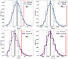 |
Fig. 5. Statistical results in 1000 simulated isotropic datasets. The left and right panels show the results from q0 and H0 investigation, respectively. The blue and purple colors represent the statistical results of isotropic analyses (isotropy) and isotropic analyses that preserve the spatial inhomogeneity of real data (isotropy RP), respectively. The black curve is the best-fitting result to the Gaussian function. The solid and vertical dashed black lines are commensurate with the mean and the standard deviation, respectively. The vertical red line shows the ALmax derived from the real data. For the isotropy analyses, the statistical significance of the real data is 1.72σ (q0) and 4.75σ (H0). For the isotropy RP analyses, the statistical significance is 1.78σ (q0) and 4.39σ (H0). |
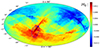 |
Fig. 6. Pseudo-color map of AL in the galactic coordinate system utilizing the HC method. The blue star and line mark the direction of the largest AL and the corresponding 1σ range in the sky. The direction and 1σ area is parameterized as ALmax,H0 (324.3 |


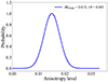 |
Fig. 7. Probability density distribution of the AL. The curve is constructed by ALmax(H0) = 0.015 ± 0.003. |
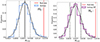 |
Fig. 8. Statistical results in 1000 simulated isotropic datasets. The blue and purple colors represent the statistical results of isotropic analyses (isotropy) and isotropic analyses that preserve the spatial inhomogeneity of real data (isotropy RP); that is, 3.42σ and 3.62σ, respectively. The black curve is the best-fitting result to the Gaussian function. The solid and vertical dashed black lines are commensurate with the mean and the standard deviation, respectively. The vertical red line shows the ALmax derived from the real data. |
All of the preferred directions that we obtained are consistent with the results of previous research that traced the anisotropy of Ωm and H0 (Antoniou & Perivolaropoulos 2010; Cai & Tuo 2012; Kalus et al. 2013; Chang & Lin 2015; Hu et al. 2020) and other dipole research (Wang & Wang 2014; Yang et al. 2014; Lin et al. 2016; Pandey 2017; Zhao et al. 2019; Dam et al. 2023), including SN Ia, quasar, GRB, and galaxy observations. However, they are different from those of Kazantzidis & Perivolaropoulos (2020), Luongo et al. (2022), Mc Conville & Colgáin (2023) and Panwar & Jain (2024), which are consistent with the CMB dipole results (Planck Collaboration I 2016, 2020). Our results are also far from those obtained by Deng & Wei (2018b), Sun & Wang (2018) and Zhao & Xia (2022). In addition, comparing them with other independent observations including the CMB dipole (Planck Collaboration I 2016, 2020), ultra-compact radio sources (Jackson 2012), dark flow (Kashlinsky et al. 2010), bulk flow (Turnbull et al. 2012; Feix et al. 2017; Watkins et al. 2023), and the galaxy cluster (Migkas et al. 2020, 2021), it is easy to find that the preferred directions that we obtained are not consistent with the CMB dipole and ultra-compact radio sources, but they coincide with the galaxy cluster and the bulk flow. For ease of understanding, we aggregated the results after 2020 with the results we obtained and marked them on the galactic coordinate system, as is shown in Fig. 9. The more detailed information is shown in Table 3. Anisotropy studies prior to 2020 can be found from Fig. 5 and Table 1 of Hu et al. (2020).
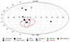 |
Fig. 9. Distribution of our preferred directions (l, b) with a 1σ range. The colored marks represent the results we obtained. The black marks show the preferred directions after 2020 given by other observations including the CMB dipole (Planck Collaboration I 2020), dark flow (Kashlinsky et al. 2010), bulk flow (Watkins et al. 2023), galaxy cluster (Migkas et al. 2020, 2021), SN-Q (Hu et al. 2020), quasar (Zhao & Xia 2021), quasar flux (Panwar & Jain 2024), Pantheon+ (Hu et al. 2024), and GRB (Zhao & Xia 2022). |
Preferred directions given by observations. DF and HC are the abbreviations for the dipole fitting method and the HC method, respectively.
6. Summary
In this paper, we combined the Padé approximation with the latest SNe Ia sample (Pantheon+) for cosmological research. First, we gave the cosmographic constraints of the third, fourth and fifth order utilizing the Padé approximations, then we found that the third-order polynomial (Padé (2, 1)) can describe the Pantheon+ sample better. The corresponding results are H0 = 72.53 ± 0.28 km/s/Mpc, q0 = −0.35 , and j0 = 0.43
 . The Padé(2, 1) polynomial that fixes j0 = 1.0 can give tighter constraints than that of the regular Padé(2, 1) polynomial. The corresponding statistical results also show that the Pantheon+ sample prefers the Padé(2, 1)(j0 = 1.0) polynomial. The comparison between the Padé approximations and the usual cosmological models shows that the Padé(2, 1)(j0 = 1) polynomials perform better than the usual cosmological models including the flat ΛCDM, non-flat ΛCDM, wCDM, CPL, and Rh = ct models.
Based on the Padé(2, 1)(j0 = 1) polynomial, we tested the cosmological principle utilizing the Pantheon+ sample and the HC method. Unlike previous works, we chose to fit the parameters H0 and q0 simultaneously. We gave the preferred directions of cosmic anisotropy; that is, (l, b) = (304.6 , −18.7
 ) for q0 and (311.1
 , −17.53
 ) for H0. The statistical isotropy analyses give the statistical significance of the real data: 1.72σ and 4.75σ for q0 and H0, respectively. The ones for the isotropy RP analyses are 1.78σ for q0 and 4.39σ for H0. The reanalyses fixing q0 = −0.55 give similar results. The preferred direction toward (l, b) = (324.3
 , −6.7
 ), and the statistical significance is 3.42σ and 3.62σ for the isotropy analyses and isotropy RP analyses, respectively. Our obtained preferred directions are consistent with each other within a 1σ range, and they are in line with the results obtained from different kinds of observations (Antoniou & Perivolaropoulos 2010; Cai & Tuo 2012; Turnbull et al. 2012; Kalus et al. 2013; Wang & Wang 2014; Yang et al. 2014; Chang & Lin 2015; Lin et al. 2016; Feix et al. 2017; Pandey 2017; Zhao et al. 2019; Hu et al. 2020; Migkas et al. 2020, 2021; Dam et al. 2023; Watkins et al. 2023). Of course, there also exist some inconsistent results (Jackson 2012; Planck Collaboration I 2016, 2020; Deng & Wei 2018b; Sun & Wang 2018; Kazantzidis & Perivolaropoulos 2020; Abdalla et al. 2022; Luongo et al. 2022; Mc Conville & Colgáin 2023; Panwar & Jain 2024). In short, the Padé approximation can be combined well with the HC method and applied to the study of cosmic anisotropy. The results show that relatively obvious anisotropic signals were found from the Pantheon+ sample. In order to better understand this signal, further analysis is still needed in the future.
Acknowledgments
We thank the anonymous referee for constructive comments. This work was supported by the National Natural Science Foundation of China (grant No. 12273009), the China Manned Spaced Project (CMS-CSST-2021-A12), Jiangsu Funding Program for Excellent Postdoctoral Talent (20220ZB59), Project funded by China Postdoctoral Science Foundation (2022M721561), Yunnan Youth Basic Research Projects (202001AU070013) and National Natural Science Foundation of China (grant No. 12373026).
References
- Abdalla, E., Abellán, G. F., Aboubrahim, A., et al. 2022, J. High Energy Astrophys., 34, 49 [NASA ADS] [CrossRef] [Google Scholar]
- Adil, S. A., Akarsu, Ö., Di Valentino, E., et al. 2024, Phys. Rev. D, 109, 023527 [CrossRef] [Google Scholar]
- Akaike, H. 1974, IEEE Trans. Automatic Control, 19, 716 [CrossRef] [Google Scholar]
- Akarsu, O., Dereli, T., & Katırcı, N. 2022, J. Phys. Conf. Ser., 2191, 012001 [NASA ADS] [CrossRef] [Google Scholar]
- Akarsu, Ö., Di Valentino, E., Kumar, S., Özyiğit, M., & Sharma, S. 2023, Phys. Dark Univ., 39, 101162 [NASA ADS] [CrossRef] [Google Scholar]
- Antoniou, I., & Perivolaropoulos, L. 2010, JCAP, 2010, 012 [NASA ADS] [CrossRef] [Google Scholar]
- Bargiacchi, G., Risaliti, G., Benetti, M., et al. 2021, A&A, 649, A65 [NASA ADS] [CrossRef] [EDP Sciences] [Google Scholar]
- Bengaly, C. A. P., Alcaniz, J. S., & Pigozzo, C. 2024, Phys. Rev. D, 109, 123533 [CrossRef] [Google Scholar]
- Bennett, C. L., Larson, D., Weiland, J. L., et al. 2013, ApJS, 208, 20 [Google Scholar]
- Betoule, M., Kessler, R., Guy, J., et al. 2014, A&A, 568, A22 [NASA ADS] [CrossRef] [EDP Sciences] [Google Scholar]
- Bhanja, S., Mandal, G., Al Mamon, A., & Biswas, S. K. 2023, JCAP, 2023, 050 [CrossRef] [Google Scholar]
- Bousis, D., & Perivolaropoulos, L. 2024, ArXiv e-prints [arXiv:2405.07039] [Google Scholar]
- Brout, D., Scolnic, D., Popovic, B., et al. 2022, ApJ, 938, 110 [NASA ADS] [CrossRef] [Google Scholar]
- Cai, R.-G., & Tuo, Z.-L. 2012, JCAP, 2012, 004 [Google Scholar]
- Caldwell, R. R., & Kamionkowski, M. 2004, JCAP, 2004, 009 [NASA ADS] [CrossRef] [Google Scholar]
- Cao, S., & Ratra, B. 2023, Phys. Rev. D, 107, 103521 [NASA ADS] [CrossRef] [Google Scholar]
- Capozziello, S., D’Agostino, R., & Luongo, O. 2018a, MNRAS, 476, 3924 [NASA ADS] [CrossRef] [Google Scholar]
- Capozziello, S., D’Agostino, R., & Luongo, O. 2018b, JCAP, 2018, 008 [CrossRef] [Google Scholar]
- Capozziello, S., Ruchika, & Sen, A. A. 2019a, MNRAS, 484, 4484 [NASA ADS] [CrossRef] [Google Scholar]
- Capozziello, S., D’Agostino, R., & Luongo, O. 2019b, Int. J. Mod. Phys. D, 28, 1930016 [NASA ADS] [CrossRef] [Google Scholar]
- Capozziello, S., D’Agostino, R., & Luongo, O. 2020, MNRAS, 494, 2576 [NASA ADS] [CrossRef] [Google Scholar]
- Carr, A., Davis, T. M., Scolnic, D., et al. 2022, PASA, 39, e046 [NASA ADS] [CrossRef] [Google Scholar]
- Carroll, S. M. 2001, Liv. Rev. Relativ., 4, 1 [NASA ADS] [CrossRef] [Google Scholar]
- Chang, Z., & Lin, H.-N. 2015, MNRAS, 446, 2952 [Google Scholar]
- Chang, Z., Lin, H.-N., Zhao, Z.-C., & Zhou, Y. 2018, Chin. Phys. C, 42, 115103 [NASA ADS] [CrossRef] [Google Scholar]
- Chen, Y., Kumar, S., Ratra, B., & Xu, T. 2024, ApJ, 964, L4 [NASA ADS] [CrossRef] [Google Scholar]
- Chevallier, M., & Polarski, D. 2001, Int. J. Modern Phys. D, 10, 213 [NASA ADS] [CrossRef] [Google Scholar]
- Chiba, T., & Nakamura, T. 1998, in 19th Texas Symposium on Relativistic Astrophysics and Cosmology, eds. J. Paul, T. Montmerle, & E. Aubourg, 276 [Google Scholar]
- Colin, J., Mohayaee, R., Rameez, M., & Sarkar, S. 2019, A&A, 631, L13 [NASA ADS] [CrossRef] [EDP Sciences] [Google Scholar]
- Dainotti, M. G., De Simone, B., Schiavone, T., et al. 2021, ApJ, 912, 150 [NASA ADS] [CrossRef] [Google Scholar]
- Dainotti, M. G., Bargiacchi, G., Bogdan, M., Capozziello, S., & Nagataki, S. 2023a, ArXiv e-prints [arXiv:2303.06974] [Google Scholar]
- Dainotti, M. G., Bargiacchi, G., Bogdan, M., et al. 2023b, ApJ, 951, 63 [CrossRef] [Google Scholar]
- Dam, L., Lewis, G. F., & Brewer, B. J. 2023, MNRAS, 525, 231 [NASA ADS] [CrossRef] [Google Scholar]
- Demianski, M., Piedipalumbo, E., Sawant, D., & Amati, L. 2017, A&A, 598, A113 [NASA ADS] [CrossRef] [EDP Sciences] [Google Scholar]
- Deng, H.-K., & Wei, H. 2018a, Eur. Phys. J. C, 78, 755 [NASA ADS] [CrossRef] [Google Scholar]
- Deng, H.-K., & Wei, H. 2018b, Phys. Rev. D, 97, 123515 [NASA ADS] [CrossRef] [Google Scholar]
- dos Santos, F. B. M. 2023, JCAP, 2023, 039 [CrossRef] [Google Scholar]
- Dunsby, P. K. S., & Luongo, O. 2016, Int. J. Geom. Methods Mod. Phys., 13, 1630002 [Google Scholar]
- Favale, A., Gómez-Valent, A., & Migliaccio, M. 2023, MNRAS, 523, 3406 [NASA ADS] [CrossRef] [Google Scholar]
- Feix, M., Branchini, E., & Nusser, A. 2017, MNRAS, 468, 1420 [NASA ADS] [CrossRef] [Google Scholar]
- Ferreira, P. D. S. & Quartin, M., 2021, Phys. Rev. D, 104, 063503 [NASA ADS] [CrossRef] [Google Scholar]
- Ghosh, S., Kothari, R., Jain, P., & Rath, P. K. 2016, JCAP, 2016, 046 [CrossRef] [Google Scholar]
- Gómez-Valent, A., Mavromatos, N. E., & Solà Peracaula, J. 2024, CQG, 41, 015026 [CrossRef] [Google Scholar]
- Gruber, C., & Luongo, O. 2014, Phys. Rev. D, 89, 103506 [NASA ADS] [CrossRef] [Google Scholar]
- Hansen, F. K., Banday, A. J., & Górski, K. M. 2004, MNRAS, 354, 641 [NASA ADS] [CrossRef] [Google Scholar]
- Horstmann, N., Pietschke, Y., & Schwarz, D. J. 2022, A&A, 668, A34 [NASA ADS] [CrossRef] [EDP Sciences] [Google Scholar]
- Hu, J. P., & Wang, F. Y. 2022a, A&A, 661, A71 [NASA ADS] [CrossRef] [EDP Sciences] [Google Scholar]
- Hu, J. P., & Wang, F. Y. 2022b, MNRAS, 517, 576 [NASA ADS] [CrossRef] [Google Scholar]
- Hu, J. P., Wang, Y. Y., & Wang, F. Y. 2020, A&A, 643, A93 [EDP Sciences] [Google Scholar]
- Hu, J. P., Wang, F. Y., & Dai, Z. G. 2021, MNRAS, 507, 730 [NASA ADS] [CrossRef] [Google Scholar]
- Hu, J. P., Wang, Y. Y., Hu, J., & Wang, F. Y. 2024, A&A, 681, A88 [NASA ADS] [CrossRef] [EDP Sciences] [Google Scholar]
- Jackson, J. C. 2012, MNRAS, 426, 779 [CrossRef] [Google Scholar]
- Jia, X. D., Hu, J. P., & Wang, F. Y. 2023, A&A, 674, A45 [NASA ADS] [CrossRef] [EDP Sciences] [Google Scholar]
- Jia, X. D., Hu, J. P., & Wang, F. Y. 2024, ArXiv e-prints [arXiv:2406.02019] [Google Scholar]
- Kalbouneh, B., Marinoni, C., & Bel, J. 2023, Phys. Rev. D, 107, 023507 [NASA ADS] [CrossRef] [Google Scholar]
- Kalbouneh, B., Marinoni, C., & Maartens, R. 2024, ArXiv e-prints [arXiv:2401.12291] [Google Scholar]
- Kalus, B., Schwarz, D. J., Seikel, M., & Wiegand, A. 2013, A&A, 553, A56 [NASA ADS] [CrossRef] [EDP Sciences] [Google Scholar]
- Kashlinsky, A., Atrio-Barandela, F., Ebeling, H., Edge, A., & Kocevski, D. 2010, ApJ, 712, L81 [Google Scholar]
- Kazantzidis, L., & Perivolaropoulos, L. 2020, Phys. Rev. D, 102, 023520 [Google Scholar]
- Koksbang, S. M. 2021, Phys. Rev. Lett., 126, 231101 [NASA ADS] [CrossRef] [Google Scholar]
- Krishnan, C., Colgáin, E. Ó., Ruchika, Sen A. A., Sheikh-Jabbari, M. M., & Yang, T., 2020, Phys. Rev. D, 102, 103525 [NASA ADS] [CrossRef] [Google Scholar]
- Krishnan, C., Mohayaee, R., Colgáin, E. Ó., Sheikh-Jabbari, M. M., & Yin, L. 2022, Phys. Rev. D, 105, 063514 [NASA ADS] [CrossRef] [Google Scholar]
- Kumar, S., Nunes, R. C., Pan, S., & Yadav, P. 2023, Phys. Dark Univ., 42, 101281 [NASA ADS] [CrossRef] [Google Scholar]
- Kumar Aluri, P., Cea, P., Chingangbam, P., et al. 2023, CQG, 40, 094001 [NASA ADS] [CrossRef] [Google Scholar]
- Li, Z., Zhang, B., & Liang, N. 2023, MNRAS, 521, 4406 [CrossRef] [Google Scholar]
- Lin, H.-N., Wang, S., Chang, Z., & Li, X. 2016, MNRAS, 456, 1881 [NASA ADS] [CrossRef] [Google Scholar]
- Linder, E. V. 2003, Phys. Rev. Lett., 90, 091301 [Google Scholar]
- Litvinov, G. 1993, Russ. J. Math. Phys., 36, 313 [Google Scholar]
- Liu, Y., Yu, H., & Wu, P. 2024, Phys. Rev. D, 110, L021304 [CrossRef] [Google Scholar]
- Lovick, T., Dhawan, S., & Handley, W. 2023, ArXiv e-prints [arXiv:2312.02075] [Google Scholar]
- Luongo, O., Muccino, M., Colgáin, E. Ó., Sheikh-Jabbari, M. M., & Yin, L. 2022, Phys. Rev. D, 105, 103510 [NASA ADS] [CrossRef] [Google Scholar]
- Lusso, E., Piedipalumbo, E., Risaliti, G., et al. 2019, A&A, 628, L4 [NASA ADS] [CrossRef] [EDP Sciences] [Google Scholar]
- Malekjani, M., Mc Conville, R., Colgáin, Ó. E., Pourojaghi, S., & Sheikh-Jabbari, M. M., 2024, Eur. Phys. J. C, 84, 317 [NASA ADS] [CrossRef] [Google Scholar]
- Mc Conville, R., Colgáin, Ó. E., 2023, Phys. Rev. D, 108, 123533 [CrossRef] [Google Scholar]
- Melia, F., & Shevchuk, A. S. H. 2012, MNRAS, 419, 2579 [NASA ADS] [CrossRef] [Google Scholar]
- Migkas, K. 2024, ArXiv e-prints [arXiv:2406.01752] [Google Scholar]
- Migkas, K., Schellenberger, G., Reiprich, T. H., et al. 2020, A&A, 636, A15 [NASA ADS] [CrossRef] [EDP Sciences] [Google Scholar]
- Migkas, K., Pacaud, F., Schellenberger, G., et al. 2021, A&A, 649, A151 [NASA ADS] [CrossRef] [EDP Sciences] [Google Scholar]
- Milaković, D., Lee, C. C., Molaro, P., & Webb, J. K. 2023, Mem. Soc. Astron. It., 94, 270 [Google Scholar]
- Millon, M., Galan, A., Courbin, F., et al. 2020, A&A, 639, A101 [NASA ADS] [CrossRef] [EDP Sciences] [Google Scholar]
- Nyagisera, R. N., Wamalwa, D., Rapando, B., Awino, C., & Mageto, M. 2024, Astronomy, 3, 43 [NASA ADS] [CrossRef] [Google Scholar]
- Pandey, B. 2017, MNRAS, 468, 1953 [NASA ADS] [CrossRef] [Google Scholar]
- Panwar, M., & Jain, P. 2024, JCAP, 2024, 019 [CrossRef] [Google Scholar]
- Pastén, E., & Cárdenas, V. H. 2023, Phys. Dark Univ., 40, 101224 [CrossRef] [Google Scholar]
- Patel, D., & Desmond, H. 2024, ArXiv e-prints [arXiv:2404.06617] [Google Scholar]
- Perivolaropoulos, L. 2023, Phys. Rev. D, 108, 063509 [NASA ADS] [CrossRef] [Google Scholar]
- Perivolaropoulos, L., & Skara, F. 2022, New Astron. Rev., 95, 101659 [CrossRef] [Google Scholar]
- Perivolaropoulos, L., & Skara, F. 2023, MNRAS, 520, 5110 [NASA ADS] [CrossRef] [Google Scholar]
- Planck Collaboration I. 2016, A&A, 594, A1 [NASA ADS] [CrossRef] [EDP Sciences] [Google Scholar]
- Planck Collaboration I. 2020, A&A, 641, A1 [NASA ADS] [CrossRef] [EDP Sciences] [Google Scholar]
- Poulin, V., Bernal, J. L., Kovetz, E. D., & Kamionkowski, M. 2023, Phys. Rev. D, 107, 123538 [NASA ADS] [CrossRef] [Google Scholar]
- Pourojaghi, S., Zabihi, N. F., & Malekjani, M. 2022, Phys. Rev. D, 106, 123523 [NASA ADS] [CrossRef] [Google Scholar]
- Qi, J.-Z., Meng, P., Zhang, J.-F., & Zhang, X. 2023, Phys. Rev. D, 108, 063522 [NASA ADS] [CrossRef] [Google Scholar]
- Rezaei, M., Pour-Ojaghi, S., & Malekjani, M. 2020, ApJ, 900, 70 [NASA ADS] [CrossRef] [Google Scholar]
- Riess, A. G., Strolger, L.-G., Tonry, J., et al. 2004, ApJ, 607, 665 [NASA ADS] [CrossRef] [Google Scholar]
- Riess, A. G., Yuan, W., Macri, L. M., et al. 2022, ApJ, 934, L7 [NASA ADS] [CrossRef] [Google Scholar]
- Risaliti, G., & Lusso, E. 2019, Nat. Astron., 3, 272 [Google Scholar]
- Sako, M., Bassett, B., Becker, A. C., et al. 2018, PASP, 130, 064002 [NASA ADS] [CrossRef] [Google Scholar]
- Schwarz, D. J., & Weinhorst, B. 2007, A&A, 474, 717 [NASA ADS] [CrossRef] [EDP Sciences] [Google Scholar]
- Schwarz, G. 1978, Ann. Stat., 6, 461 [Google Scholar]
- Scolnic, D., Brout, D., Carr, A., et al. 2022, ApJ, 938, 113 [NASA ADS] [CrossRef] [Google Scholar]
- Scolnic, D., Riess, A. G., Wu, J., et al. 2023, ApJ, 954, L31 [NASA ADS] [CrossRef] [Google Scholar]
- Scolnic, D. M., Jones, D. O., Rest, A., et al. 2018, ApJ, 859, 101 [NASA ADS] [CrossRef] [Google Scholar]
- Simon, T. 2024, Phys. Rev. D, 110, 023528 [CrossRef] [Google Scholar]
- Singal, A. K. 2023, MNRAS, 524, 3636 [NASA ADS] [CrossRef] [Google Scholar]
- Solà Peracaula, J., Gómez-Valent, A., de Cruz Pérez, J., & Moreno-Pulido, C. 2023, Universe, 9, 262 [CrossRef] [Google Scholar]
- Steven, G. K., & Harold, R. P. 1992, Birkhuser Advanced Texts, 39, 373 [Google Scholar]
- Sun, Z. Q., & Wang, F. Y. 2018, MNRAS, 478, 5153 [NASA ADS] [CrossRef] [Google Scholar]
- Tang, L., Lin, H.-N., Liu, L., & Li, X. 2023, Chin. Phys. C, 47, 125101 [NASA ADS] [CrossRef] [Google Scholar]
- Turnbull, S. J., Hudson, M. J., Feldman, H. A., et al. 2012, MNRAS, 420, 447 [Google Scholar]
- Tutusaus, I., Kunz, M., & Favre, L. 2023, ArXiv e-prints [arXiv:2311.16862] [Google Scholar]
- Valdez, G. A. C., Quintanilla, C., García-Aspeitia, M. A., Hernández-Almada, A., & Motta, V. 2023, Eur. Phys. J. C, 83, 442 [NASA ADS] [CrossRef] [Google Scholar]
- Van Raamsdonk, M., & Waddell, C. 2024, JCAP, 2024, 047 [CrossRef] [Google Scholar]
- Visser, M. 2004, CQG, 21, 2603 [NASA ADS] [CrossRef] [Google Scholar]
- Visser, M. 2015, CQG, 32, 135007 [NASA ADS] [CrossRef] [Google Scholar]
- Vitagliano, V., Xia, J.-Q., Liberati, S., & Viel, M. 2010, JCAP, 2010, 005 [CrossRef] [Google Scholar]
- Wang, F. Y., Dai, Z. G., & Qi, S. 2009, A&A, 507, 53 [NASA ADS] [CrossRef] [EDP Sciences] [Google Scholar]
- Wang, F. Y., Hu, J. P., Zhang, G. Q., & Dai, Z. G. 2022, ApJ, 924, 97 [NASA ADS] [CrossRef] [Google Scholar]
- Wang, J. S., & Wang, F. Y. 2014, MNRAS, 443, 1680 [NASA ADS] [CrossRef] [Google Scholar]
- Watkins, R., Allen, T., Bradford, C. J., et al. 2023, MNRAS, 524, 1885 [NASA ADS] [CrossRef] [Google Scholar]
- Wei, H., Yan, X.-P., & Zhou, Y.-N. 2014, JCAP, 2014, 045 [CrossRef] [Google Scholar]
- Weinberg, S. 1972, Gravitation and Cosmology: Principles and Applications of the General Theory of Relativity [Google Scholar]
- Wong, K. C., Suyu, S. H., Chen, G. C. F., et al. 2020, MNRAS, 498, 1420 [Google Scholar]
- Yadav, V. 2023, Phys. Dark Univ., 42, 101365 [NASA ADS] [CrossRef] [Google Scholar]
- Yadav, V., Yadav, S. K., & Rajpal, X. X. 2024, ArXiv e-prints [arXiv:2402.16885] [Google Scholar]
- Yang, T., Banerjee, A., Colgáin, Ó. E., 2020, Phys. Rev. D, 102, 123532 [NASA ADS] [CrossRef] [Google Scholar]
- Yang, X., Wang, F. Y., & Chu, Z. 2014, MNRAS, 437, 1840 [NASA ADS] [CrossRef] [Google Scholar]
- Yershov, V. N. 2023, Universe, 9, 204 [NASA ADS] [CrossRef] [Google Scholar]
- Yu, H., Ratra, B., & Wang, F.-Y. 2018, ApJ, 856, 3 [NASA ADS] [CrossRef] [Google Scholar]
- Zhang, M.-J., Li, H., & Xia, J.-Q. 2017, Eur. Phys. J. C, 77, 434 [NASA ADS] [CrossRef] [Google Scholar]
- Zhao, D., & Xia, J.-Q. 2021, Eur. Phys. J. C, 81, 694 [NASA ADS] [CrossRef] [Google Scholar]
- Zhao, D., & Xia, J.-Q. 2022, MNRAS, 511, 5661 [NASA ADS] [CrossRef] [Google Scholar]
- Zhao, D., Zhou, Y., & Chang, Z. 2019, MNRAS, 486, 5679 [Google Scholar]
- Zhou, Y., Zhao, Z.-C., & Chang, Z. 2017, ApJ, 847, 86 [NASA ADS] [CrossRef] [Google Scholar]
Appendix A: 1σ and 2σ contours in the 2-D parameter space utilizing different cosmological models
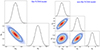 |
Fig. A.1. Confidence contours (1σ and 2σ) and marginalized likelihood distributions for the parameters space (Ωm, ΩΛ and H0) employing the Pantheon+ sample in the ΛCDM models. Left and right panels show the results from the flat and non-flat ΛCDM models, respectively. |
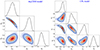 |
Fig. A.2. Confidence contours (1σ and 2σ) and marginalized likelihood distributions for the parameters space (Ωm, w0, wa and H0) employing the Pantheon+ sample in the dark energy models. Left and right panels show the results from the wCDM and CPL models, respectively. |
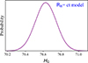 |
Fig. A.3. Probability distribution of H0 employing the Pantheon+ sample from the Rh = ct model. |
All Tables
Best-fitting results at the 68 percent confidence level using the Pantheon+ sample under different expansion methods and cosmological models.
Statistical results with respect to the reference flat ΛCDM model by utilizing the AIC and BIC statistical criteria.
Preferred directions given by observations. DF and HC are the abbreviations for the dipole fitting method and the HC method, respectively.
All Figures
|
Fig. 1. Basic information about the Pantheon+ sample. The left panel shows the cumulative redshift distribution. The right panel shows the location of different redshift SNe in the galactic coordinate system. |
| In the text | |
|
Fig. 2. Confidence contours (1σ and 2σ) and marginalized likelihood distributions for the parameter space (H0, q0, j0, and s0) from the Pantheon+ sample utilizing the Padé approximations including Padé(2, 1), Padé(2, 2), Padé(3, 2), and Padé(2, 1)(j0 = 1) polynomials. |
| In the text | |
|
Fig. 3. Pseudo-color map of AL in the galactic coordinate system utilizing the HC method. The upper and lower panels show the results of q0 and H0, respectively. The blue star and line mark the direction of the largest AL and the corresponding 1σ range in the sky. The corresponding directions and 1σ areas are parameterized as ALmax,q0 (304.6 |
| In the text | |
|
Fig. 4. Probability density distribution of the AL. The left and right panels are plotted by using ALmax(q0) = 0.34 ± 0.08 and ALmax(H0) = 0.028 ± 0.004), respectively. |
| In the text | |
|
Fig. 5. Statistical results in 1000 simulated isotropic datasets. The left and right panels show the results from q0 and H0 investigation, respectively. The blue and purple colors represent the statistical results of isotropic analyses (isotropy) and isotropic analyses that preserve the spatial inhomogeneity of real data (isotropy RP), respectively. The black curve is the best-fitting result to the Gaussian function. The solid and vertical dashed black lines are commensurate with the mean and the standard deviation, respectively. The vertical red line shows the ALmax derived from the real data. For the isotropy analyses, the statistical significance of the real data is 1.72σ (q0) and 4.75σ (H0). For the isotropy RP analyses, the statistical significance is 1.78σ (q0) and 4.39σ (H0). |
| In the text | |
|
Fig. 6. Pseudo-color map of AL in the galactic coordinate system utilizing the HC method. The blue star and line mark the direction of the largest AL and the corresponding 1σ range in the sky. The direction and 1σ area is parameterized as ALmax,H0 (324.3 |
| In the text | |
|
Fig. 7. Probability density distribution of the AL. The curve is constructed by ALmax(H0) = 0.015 ± 0.003. |
| In the text | |
|
Fig. 8. Statistical results in 1000 simulated isotropic datasets. The blue and purple colors represent the statistical results of isotropic analyses (isotropy) and isotropic analyses that preserve the spatial inhomogeneity of real data (isotropy RP); that is, 3.42σ and 3.62σ, respectively. The black curve is the best-fitting result to the Gaussian function. The solid and vertical dashed black lines are commensurate with the mean and the standard deviation, respectively. The vertical red line shows the ALmax derived from the real data. |
| In the text | |
|
Fig. 9. Distribution of our preferred directions (l, b) with a 1σ range. The colored marks represent the results we obtained. The black marks show the preferred directions after 2020 given by other observations including the CMB dipole (Planck Collaboration I 2020), dark flow (Kashlinsky et al. 2010), bulk flow (Watkins et al. 2023), galaxy cluster (Migkas et al. 2020, 2021), SN-Q (Hu et al. 2020), quasar (Zhao & Xia 2021), quasar flux (Panwar & Jain 2024), Pantheon+ (Hu et al. 2024), and GRB (Zhao & Xia 2022). |
| In the text | |
|
Fig. A.1. Confidence contours (1σ and 2σ) and marginalized likelihood distributions for the parameters space (Ωm, ΩΛ and H0) employing the Pantheon+ sample in the ΛCDM models. Left and right panels show the results from the flat and non-flat ΛCDM models, respectively. |
| In the text | |
|
Fig. A.2. Confidence contours (1σ and 2σ) and marginalized likelihood distributions for the parameters space (Ωm, w0, wa and H0) employing the Pantheon+ sample in the dark energy models. Left and right panels show the results from the wCDM and CPL models, respectively. |
| In the text | |
|
Fig. A.3. Probability distribution of H0 employing the Pantheon+ sample from the Rh = ct model. |
| In the text | |
Current usage metrics show cumulative count of Article Views (full-text article views including HTML views, PDF and ePub downloads, according to the available data) and Abstracts Views on Vision4Press platform.
Data correspond to usage on the plateform after 2015. The current usage metrics is available 48-96 hours after online publication and is updated daily on week days.
Initial download of the metrics may take a while.