| Issue |
A&A
Volume 678, October 2023
|
|
|---|---|---|
| Article Number | A181 | |
| Number of page(s) | 10 | |
| Section | Cosmology (including clusters of galaxies) | |
| DOI | https://doi.org/10.1051/0004-6361/202347143 | |
| Published online | 18 October 2023 | |
CHEX-MATE: X-ray absorption and molecular content of the interstellar medium toward galaxy clusters
1
Università degli studi di Roma ‘Tor Vergata’, Via della Ricerca Scientifica, 1, 00133 Roma, Italy
e-mail: This email address is being protected from spambots. You need JavaScript enabled to view it.
2
INFN, Sezione di Roma 2, Università degli Studi di Roma Tor Vergata, Via della Ricerca Scientifica, 1, Roma, Italy
3
INAF, IASF-Milano, Via A. Corti 12, 20133 Milano, Italy
4
Department of Physics and Astronomy, Michigan State University, 567 Wilson Road, East Lansing, MI 48824, USA
5
Department of Astronomy, University of Geneva, Ch. d’Ecogia 16, 1290 Versoix, Switzerland
6
INAF, Osservatorio di Astrofisica e Scienza dello Spazio, Via Pietro Gobetti 93/3, 40129 Bologna, Italy
7
INFN, Sezione di Bologna, Viale Berti Pichat 6/2, 40127 Bologna, Italy
8
Jodrell Bank Centre for Astrophysics, Department of Physics and Astronomy, School of Natural Sciences, The University of Manchester, Oxford Road, Manchester M13 9PL, UK
9
Center for Astrophysics | Harvard & Smithsonian, 60 Garden Street, Cambridge, MA 02138, USA
10
HH Wills Physics Laboratory, University of Bristol, Tyndall Ave, Bristol BS8 1TL, UK
11
IRAP, Université de Toulouse, CNRS, CNES, UT3-UPS, Toulouse, France
12
Université Paris-Saclay, Université Paris Cité, CEA, CNRS, AIM, 91191 Gif-sur-Yvette, France
Received:
9
June
2023
Accepted:
28
July
2023
Abstract
The X-ray spectrum of extragalactic sources, such as galaxy clusters, is affected by the photo-absorption of various components of the Galactic interstellar medium (ISM). The resulting spectral distortion contributes to the systematics of cluster temperature measurements. It essentially depends on the neutral (atomic+molecular) Galactic hydrogen density column, NH, which remains challenging to map across the sky in the lack of a straightforward tracer of the molecular gas phase in the ISM. Combining data from the HI4PI and Planck HFI sky surveys, we investigate the mass fraction of molecular gas across the line of sight of CHEX-MATE galaxy clusters by searching for thermal dust emission excess with respects to the neutral atomic hydrogen density column, NHI. Consistent with earlier studies of the ISM based on IRAS and Planck data, we detect dust emission excess along the line of sight of some members of the CHEX-MATE cluster catalogue that are mostly localised behind dense ISM regions. We find that the CHEX-MATE cluster catalogue can be divided into three categories: 40% of members are located behind low NHI regions where the molecular mass fraction is negligible, 40% of members are located behind intermediate NHI regions where the molecular gas fraction would reach 5% on average, and the remaining 20% of members are located behind high NHI regions that locally exhibit even higher molecular gas fractions. The apparent cluster temperature shifts associated with the molecular content of the ISM are about 1% or less for most CHEX-MATE clusters, but can exceed 5% in the highest NHI regions.
Key words: dust / extinction / galaxies: clusters: intracluster medium
© The Authors 2023
 Open Access article, published by EDP Sciences, under the terms of the Creative Commons Attribution License (https://creativecommons.org/licenses/by/4.0), which permits unrestricted use, distribution, and reproduction in any medium, provided the original work is properly cited.
This article is published in open access under the Subscribe to Open model. This email address is being protected from spambots. You need JavaScript enabled to view it. to support open access publication.
1. Introduction
The radiation of extragalactic X-ray sources is partly absorbed by the interstellar medium (ISM) of the Milky Way galaxy. Specifically, X-ray absorption by atoms, molecules, and grains that populate the ISM is quantified by specific photo-ionisation or photo-absorption cross sections, σgas, σmol, and σgrains, yielding a total effective photo-absorption cross section that depends on the energy, e, and follows
 (1)
(1)
Because σISM is energy dependent, the spectral shape of X-ray sources is affected by this photo-absorption. The resulting spectral distortion can be modelled as
 (2)
(2)
where the ISM photo-absorption cross section is conventionally renormalised with respect to the neutral (atomic+molecular) hydrogen density column: NH = NHI + 2NH2. Given a photo-absorption cross section, spectroscopic studies of extragalactic sources thus take ISM absorption into account via an a priori knowledge of the hydrogen density column along the line of sight or a joint fit of the NH parameter with the intrinsic shape of the source spectrum, Is. While the atomic contribution, NHI, to the total hydrogen density column can be traced from radio surveys of the 21 cm emission line, one difficulty in estimating NH is the observational lack of a continuous mapping of the molecular hydrogen density column across the sky. Except for direct measurements of (far)-UV absorption lines limited to localised background objects (Savage et al. 1977; Gillmon et al. 2006; Rachford et al. 2002, 2009), the molecular hydrogen density column, NH2, can only be indirectly traced from maps of rotational emission lines of CO (e.g. Dame et al. 2001), or combinations of NHI surveys with thermal dust emission maps, as detailed below.
Early UV spectroscopic observations of stars across the sky have revealed an invariance of the neutral hydrogen density column to the Galactic dust extinction ratio NH/E(B − V) (Bohlin et al. 1978), suggesting that the abundance of dust grains is homogeneous in the ISM, regardless of the mass fraction of molecular hydrogen, f = 2NH2/(NHI + 2NH2). Subsequent IR and sub-millimeter sky surveys (IRAS1 and COBE-FIRAS2) have shown that the thermal dust emission at high Galactic latitude can be modelled as a greybody with characteristic temperature T ∼ 17.5 K, whose emission appears to be spatially correlated with the neutral atomic hydrogen density column for low NHI values (Boulanger et al. 1996; Boulanger & Perault 1988). The dust-gas correlation then exhibits a change in the slope and a larger scatter for NHI values higher than about 5 × 1020 cm−2, a break that coincides with the threshold above which the fraction of molecular hydrogen becomes significant in UV surveys. These and more recent observations support a picture in which the dust emission traces the (atomic+molecular) hydrogen density column at high Galactic latitude. In this picture, the molecular hydrogen locally survives photo-dissociation within diffuse clouds because it is self-shielded from the interstellar radiation field (ISRF). The presence of diffuse molecular clouds, characterised by f ≥ 0.1 (Wakelam et al. 2017), can finally be inferred in sky regions in which the thermal dust emission exceeds the tight correlation observed for the lowest NHI values (Desert et al. 1988; Reach et al. 1998; Röhser et al. 2016).
In galaxy cluster observations, temperature estimates are prone to degeneracies with NH measurements, particularly in the regimes of high temperature and/or low signal-to-noise ratio (S/N), which tend to favour the use of independent measurements of the NH value when available. Earlier cluster studies have used NH priors from neutral atomic hydrogen surveys, gamma-ray burst X-ray spectra (e.g. Schellenberger et al. 2015; Lovisari & Reiprich 2019), or thermal dust models in sky regions in which spectroscopic NH measurements seemed to show inconsistencies with NHI (e.g. Pointecouteau et al. 2004; Bourdin et al. 2011; Reiprich et al. 2021). It is worth mentioning that these models might have to disentangle the Galactic and intra-cluster dust emissions. In this regard, stacked IRAS and Planck observations of optical and Sunyaev-Zel’dovich (SZ) cluster catalogues that extend out to redshift 1 have evidenced a dust emission originating from clusters, whose spectral shape is expected to mimic the spectral energy distribution (SED) of Galactic thermal dust (Montier & Giard 2005; Planck Collaboration Int. XLIII 2016). The redshift dependence of infrared cluster luminosities and the SED of the intra-cluster dust emission have been shown to be compatible with an emission mechanism related to the star formation in early-type cluster galaxies (Roncarelli et al. 2010). On the other hand, constraints derived from quasar extinctions behind SDSS clusters a priori leave little room for a remaining diffuse dust emission (Giard et al. 2008).
The Planck mission has covered the Galactic emission of thermal dust at an angular resolution of 5 arcmin down to sub-millimetre wavelengths, thus providing us with new constraints on sky maps of spectroscopic parameters, such as dust optical depth, spectral index, and temperature (Planck Collaboration XI 2014; Meisner & Finkbeiner 2015). Its spectral coverage also permitted us to map the SZ signature of hot baryons across the sky (Planck Collaboration XXII 2016), and to detect 1000 galaxy clusters up to redshift 1 (Planck Collaboration XXVII 2016). The Cluster HEritage project with XMM-Newton3 Mass Assembly and Thermodynamics at the Endpoint of structure formation (CHEX-MATE; CHEX-MATE Collaboration 2021) is an X-ray follow-up of the Planck catalogue of SZ sources. It probes both a population of nearby objects (z < 0.2) and the most massive galaxy clusters at z < 0.6. Combining Planck data with data from HI4PI, the NHI sky survey of highest angular resolution and sensitivity available, this work will provide NH priors for the X-ray analysis of CHEX-MATE clusters by (1) measuring the average neutral density column, and (2) estimating the molecular gas fraction of the ISM in the cluster lines of sight. We present our Planck+HI4PI+LAB data set in Sect. 3, discuss the results we obtained for NH and its molecular content for the CHEX-MATE cluster catalogue in Sect. 4, speculate how these priors could inform spectroscopic analyses of CHEX-MATE clusters, and present our conclusions in Sect. 5. Hereafter, intra-cluster distances are computed as angular diameter distances, assuming a Λ-CDM cosmology with H0 = 70 km s−1 Mpc−1, ΩM = 0.3, and ΩΛ = 0.7. Here, rΔ is the radius of a sphere whose matter content exceeds the critical density of its coeval universe by a factor Δ. Unless otherwise noted, confidence intervals and envelopes encompass a 68% probability.
2. Galaxy cluster sample
By design of this S/N-limited subsample of the Planck catalogue of SZ sources, the CHEX-MATE cluster population can be seen as a representative probe of the X-ray absorption at high Galactic latitudes. Specifically, the CHEX-MATE sample is composed of 120 clusters with apparent diameters θ500 in the range [3, 22] arcmin, all of which are located behind neutral atomic hydrogen column densities, NHI, in the range [1020, 1021] cm−2. These column densities exclude the densest regions of the Galactic plane and the dense molecular clouds, where molecular hydrogen is abundant, and where dust extinction permits nearly all carbon to reach the stable form of CO. The CHEX-MATE lines of sight instead tend to probe both diffuse atomic clouds, in which molecules are thought to be quickly photo-dissociated by the ISRF, and diffuse molecular clouds, in which some attenuation of the ISRF a priori allows the survival of a significant mass fraction of molecular hydrogen (see Snow & McCall 2006, for a review about diffuse interstellar clouds).
3. Observations and data preparation
This work relies on the (sub)-millimeter sky survey performed with Planck and the two radio sky surveys Leiden, Argentine, and Bonn (LAB, Kalberla et al. 2005) and HI 4π (HI4PI, HI4PI Collaboration 2016). We used Planck data registered with the High Frequency Instrument (HFI) for the second data release, which covered the full mission in 2015 (Planck Collaboration VIII 2016). Planck HFI scanned the sky at 100, 143, 217, 353, 545, and 857 GHz, with an average angular resolutions corresponding to 10, 7, 5, 5, 5, and 5 arcmin, respectively (Planck Collaboration VII 2014). The LAB survey corresponds to the final data release of observations of 21 cm emission from Galactic neutral atomic hydrogen over the entire sky, merging the Leiden-Dwingeloo Survey of the sky north of −30° (Hartmann & Burton 1997) with the Instituto Argentino de Radioastronomia Survey of the sky south of −25° (Arnal et al. 2000; Bajaja et al. 2005). The angular resolution of the combined material reaches a half-power beam width of about 0.6 sq. deg. We used sky maps of brightness temperatures registered in equispaced velocity intervals of 10 km s−1 that cover local standard-of-rest velocities in the range |v|< 450 km s−1. The HI4PI survey is based on data from the first coverage of the Effelsberg-Bonn HI Survey (EBHIS; Kerp et al. 2011) and from the third revision of the Galactic All-Sky Survey (GASS; McClure-Griffiths et al. 2009). We used an all sky NHI map of this combined survey computed from the integration of brightness temperatures measurements in a velocity interval |v|< 600 km s−1, whose angular resolution reaches 16.2 arcmin.
For self-consistency purposes in our analyses, we calibrated the antenna temperature of the HFI 857 GHz map in NHI units of the HI4PI NHI map within a sky region in which the two quantities are expected to exhibit a tight correlation. This dust-gas correlation region is characterised by low NHI values, a low contribution of intermediate- or high-velocity clouds (IVC and HVC) to the NHI values, and a low contamination from thermal SZ sources. A low NHI – low SZ sky region was first defined by combining HI4PI maps with a map of the thermal SZ effect resulting from a modified interlinear combination algorithm (MILCA; Hurier et al. 2013; Planck Collaboration XXII 2016). After projecting these maps onto a common grid with an angular resolution of 0.64 sq. deg., we defined a mask that selected NH and Compton parameter values lower than 2 × 1020 cm−2 and 10−5. Similarly to the approach presented in Planck Collaboration XI (2014), we measured the contribution of IVC and HVC characterised by |v|> 30 km s−1 to the NHI values measured for each pixel of the LAB maps, and excluded pixels for which one of these contributions exceeded a threshold of 0.1 × 1020 cm−2 from our correlation region. As shown in Fig. 1, the resulting correlation region was used to perform a linear regression of the HFI 857 GHz map with respects to the NHI values4,
 (3)
(3)
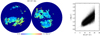 |
Fig. 1. Calibration of the antenna temperature of the HFI 857 GHz map in NHI units. Left panel: HFI 857 GHz map intensity observable within a dust-gas correlation region, characterised by low NHI values, a low contribution of intermediate- or high-velocity clouds (IVC and HVC) to the NHI values, and a low contamination from thermal SZ sources (see details in Sect. 3). Right panel: pixel-to-pixel correlation and linear regression between the HFI 857 GHz and HI4PI NHI maps in the sky region visible in the left panel. |
After correcting the HFI 857 GHz intensity map for an offset of b = 0.571 MJy sr−1, we found a proportional relation between the sky surface brightness at 857 GHz and the neutral atomic hydrogen density column of I857 = a NHI, with a = (0.0385 ± 0.0009)× MJy sr−1 × 10⁻¹⁹ cm2.
4. Data analysis
4.1. Thermal dust emission in the neighbourhood of CHEX-MATE clusters
Because galaxy clusters contaminate the spectral shape of the Galactic emission in the sub-millimeter band, modelling the thermal dust emission along their line of sight requires a specific component-separation approach. We inferred square-degree dust emission maps centred on each galaxy cluster as follows.
-
We defined a Cosmic Microwave Background (CMB) template whose spectral shape was defined as a 2.72548 K blackbody (Fixsen 2009) and whose spatial shape was inferred from a wavelet denoising of the HFI 217 GHz frequency map.
-
We defined a Galactic thermal dust template whose spectral shape, s(ν), was parametrised as the sum of two greybodies and whose spatial shape, Iν, was inferred at pixel coordinate (k, l), from a wavelet denoising of the 857 GHz HFI frequency map,
![Mathematical equation: $$ \begin{aligned}&s(\nu ) = \left[f_1 q_1/q_2 \left(\frac{\nu }{\nu _o}\right)^{\beta _{1}} B_\nu (T_1)\right.\nonumber \\&\qquad \quad \left. +(1-f_1) \left(\frac{\nu }{\nu _o}\right)^{\beta _{2}} B_\nu (T_2)\right],\nonumber \\&I_{\nu }(k,l) = I_{857}(k,l) \frac{s(\nu )}{s(857)}\cdot \end{aligned} $$](/articles/aa/full_html/2023/10/aa47143-23/aa47143-23-eq4.gif) (4)
(4)Specifically, the dust SED was parametrised using two constant spectral indices, β1 and β2, and two interdependent temperatures, T1 and T2, the highest of the two being the result of a joint fit between HFI and IRAS data, following the full-sky modelling of Meisner & Finkbeiner (2015).
-
We parametrised the dust SED via the joint fit of specific intensities of the CMB template and the greybodies of Eq. (4) to the HFI data set. This fit was performed in a cluster-centric annulus supposedly free of intra-cluster thermal dust or thermal SZ signals, delimited by the radius range [3, 6]×r5005.
A stacking of multi-frequency details reconstructed as a linear combination of CMB and Galactic thermal dust templates toward CHEX-MATE clusters is shown in Fig. 2, together with the residuals separating these templates from the HFI data set. The modelling residuals show us that the CMB and Galactic thermal dust are dominant in the radius range [3, 6]×r500. On the other hand, a thermal SZ (tSZ) distortion of CMB temperatures significantly contributes to the observed signal in the radius range [0, 3]×r500. This tSZ contribution can be modelled as a Kompaneets (non-relativistic) distortion, whose emission is spatially distributed as the projection of a cluster mass-scaled hot-gas pressure profile, which follows the parametrisation of Arnaud et al. (2010) up to a free renormalisation factor. We note that our CMB+thermal dust template fitting was performed on a high-pass filtered data set, which increased its accuracy. Specifically, we took advantage of the specificities of discrete B3-spline wavelet transforms to limit the analysis to details of angular resolutions higher than 1 sq. deg., and linearly combined these details with a low-pass filtering of the 857 GHz frequency map at an angular resolution of about 1 sq. deg. The resulting multi-frequency thermal dust template provided us with maps of the dust emission at any given frequency, that were centred on each CHEX-MATE cluster, and encompassed a sky area of diameter 12 × r500. By convention, we hereafter normalised the dust SED to the emission expected at 857 GHz and worked with the corresponding intensity maps, I857.
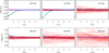 |
Fig. 2. Stacked radial profiles of the SZ signal registered toward CHEX-MATE clusters by the Planck HFI instrument. These profiles radially average HFI frequency maps that were first high-pass filtered and show details of an angular resolution higher than 1 sq. deg. As detailed in Sect. 4, the resulting SZ signal (black points) was corrected for a linear combination of CMB and Galactic thermal dust templates. The dark blue and light blue lines depict the arithmetical mean of CMB and thermal SZ templates that were fit to the data set for each individual cluster, respectively. The red lines depict the individual cluster templates associated with Galactic thermal dust. |
4.2. Thermal dust emission excesses over neutral atomic hydrogen density column
Assuming that the Galactic thermal dust emission traces the total hydrogen density column above the Galactic plane, the mass fraction of molecular hydrogen can be inferred toward CHEX-MATE clusters by comparing the dust optical depth with the neutral atomic hydrogen density column. We recall that the dust optical depth, τν, can be extracted at a frequency ν from the two-component dust SED, s(ν), via Iν = τνs(ν). Given a sky-averaged dust SED, ⟨s(ν)⟩, this allowed us to calibrate a dust intensity to NH linear relation at 857 GHz in a sky region that was assumed to be empty of molecular hydrogen (see also Sect. 2 and Eq. (3)),
 (5)
(5)
We further introduced effective dust intensities, I⟨s(857)⟩, that correct our NH-calibrated intensity maps for local variations of the dust SED,
 (6)
(6)
Using the calibration NH ≡ ϕ(I⟨s(857)⟩), we inferred based on these effective intensities NH values in the neighbourhood of each CHEX-MATE cluster. The resulting NH maps were compared with patches of the all sky NHI map provided by the HI4PI survey by extracting cluster-centric radial profiles of both quantities in the range [0, 6]×r500. For each cluster, the values of NHI and mass fractions of molecular hydrogen, f = 2NH2/(NHI + 2NH2)≡max(NH − NHI, 0)/NH were also averaged in the radius range [3, 6]×r500 and are listed in Table A.1. We discuss our results for low, intermediate, and high NHI below, which we define by values in the ranges NHI < 2 × 1020 cm−2, 2 × 1020 cm−2 < NHI < 5 × 1020 cm−2, and NHI > 5 × 1020 cm−2, respectively.
Stacked radial profiles of the neutral atomic hydrogen density column and effective dust intensities calibrated in NH units, ϕ(I⟨s(857)⟩), are shown in Fig. 3. In the lowest of the three NHI ranges, which corresponds to NHI < 2 × 1020 cm−2, radial profiles of the dust intensity exhibit a marginal gradient along the radius interval [0, 3]×r500, and remain fully consistent with the neutral atomic hydrogen density column across the radius range [0, 6]×r500. For NHI ranges that encompass values higher than 2 × 1020 cm−2, the stacked dust intensity profiles appear as flat along the radius interval [0, 3]×r500 and exhibit a significant excess with respect to the neutral atomic hydrogen density column. The two behaviours observed for average NHI values below or above 2 × 1020 cm−2 suggest that a significant mass fraction of molecular hydrogen is likely to be only detectable for individual NHI values that exceed a threshold of about 2 × 1020 cm−2.
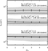 |
Fig. 3. Stacked radial profiles of the neutral atomic hydrogen density column (NHI, single lines) compared with ISM proxies of the total hydrogen density column (NH, lines with errors) for three intervals of increasing NHI values. NHI profiles radially average patches of the all-sky HI4PI survey. NH proxies, NH ≡ ϕ(I⟨s(857)⟩), are inferred from HFI measurements of the dust emission at 857 GHz, which we corrected for local variations in the dust SED (see also Eqs. (3) and (6)). The shaded areas depict the dispersions of differences between NH and NHI values. The error bars depict the uncertainties on the average values of these differences. |
The gradient of the dust intensity that we observed for low NHI values could be attributed to some marginal contamination of the Galactic thermal dust emission from CHEX-MATE clusters. The intra-cluster dust emission observed in stacked IRAS and Planck observations of optical and SZ cluster catalogues is expected to reach a few percent of the background level (Montier & Giard 2005; Planck Collaboration Int. XLIII 2016), with an apparent extension that sightly exceeds the angular size of X-ray and SZ cluster signals (Planck Collaboration XXIII 2016). To avoid any contamination from cluster galaxies, we hereafter investigate the molecular hydrogen density column toward individual CHEX-MATE clusters from the average ratio, NH/NHI, that can be measured assuming NH ≡ ϕ(I⟨s(857)⟩) in the radius range [3, 6]×r500. Histograms of the NH/NHI ratios are plotted in Fig. 4. The median values of NH/NHI for the three NHI ranges are 0.97, 1.05, and 1.13. These raw measurements include NH/NHI values above and below 1, although only values higher than one are physically meaningful. In the lowest of the three NH ranges, the NH/NHI ratios are close to or lower than one. In the intermediate NHI range, the histogram of the NH/NHI ratios peaks around the median value, 1.05. In the highest of the three NHI ranges, the NH/NHI ratios finally show larger scatter, with values that spread from 0.8 to 1.7.
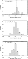 |
Fig. 4. Histograms of the thermal dust emission excesses over hydrogen density column, ϕ(I⟨s(857)⟩)/NHI, registered for each CHEX-MATE clusters in the intra-cluster radius range [3, 6]×r500. The vertical lines indicate the median values of the excesses. The lower to upper panels correspond to the three intervals of increasing NHI values that were used to plot stacked radial profiles of I857 and NHI in Fig. 3. |
5. Discussion and conclusions
5.1. Molecular mass fraction of the ISM toward CHEX-MATE clusters
By searching for dust emission excess with respect to the neutral atomic hydrogen density column, we investigated the mass fraction of molecular gas in the lines of sight toward CHEX-MATE clusters. We found a discrepancy between measurements corresponding to low and high NHI values, which we separated by a threshold of 2 × 1020 cm−2. Below the threshold of 2 × 1020 cm−2, most dust emission excess is consistent with zero. Consistent with earlier studies of the ISM based on IRAS and Planck data (Boulanger et al. 1996; Planck Collaboration XI 2014), this result could be related to the inefficiency of H2 self-shielding in the low NHI regime (Valdivia et al. 2016). Above the threshold of 2 × 1020 cm−2, most cluster lines of sight are characterised by a significant dust emission excess. Individual values of this excess exhibit a rather large scatter and no clear correlation with neutral atomic hydrogen density columns. The partial independence of these two quantities agrees with a picture in which the spatial distribution of molecular gas is specific to this gas phase. In line with this result, earlier investigations of dust emission excesses over NHI at high Galactic latitudes have suggested the presence of a specific population of molecular clouds made of cells whose apparent size does not exceed a few square degrees (Desert et al. 1988; Reach et al. 1998, 2015).
An estimate of the X-ray absorption by the Galactic ISM was provided by Willingale et al. (2013, hereafter W13). Briefly, W13 introduced an analytical modelling of spatial variations of NH2 across the sky depending on NHI and dust extinction E(B − V) as measured by the IRAS and LAB surveys. Their modelling was calibrated in various NHI bins using stacked gamma-ray burst emission spectra observed by Swift. The total hydrogen density column inferred by W13 is compared with results of the present work in Fig. 5. Our measurements of the molecular fraction in the hydrogen density column asymptotically agree with estimates of W13 toward high NHI values, but are generally lower in the low NHI regime (NHI < 2 × 1020 cm−2) and somewhat more patchy. Differences between results of the two works might be related to distinct assumptions in the analytical modelling of the molecular hydrogen density column. Specifically, at variance with the NH proxy adopted in the present work, NH ≡ ϕ(I⟨s(857)⟩), Eq. (7) of W13 introduces a non-linear dependence of NH2 on NHI and dust extinction.
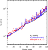 |
Fig. 5. Comparison of atomic (black) and total (dark blue) hydrogen density columns derived in this work around individual CHEX-MATE clusters with NH estimates provided by the all-sky modelling of Willingale et al. (2013). |
5.2. Perspectives for X-ray observations
X-ray emission spectra of galaxy clusters are absorbed by the Galactic ISM, which yields a spectral distortion that depends on the molecular mass fraction owing to the NH and the σISM terms of Eq. (2). The main effect of the molecular mass fraction is to increase the NH term over and above neutral atomic hydrogen density column measurements. From our investigation of the dust emission excess, we find that the CHEX-MATE cluster catalogue can be divided into three categories: 40% of the sample members are located behind low NHI regions where the molecular mass fraction is negligible, 40% are located behind intermediate NHI regions where the molecular gas fraction reaches 5% on average, and the remaining 20% are located behind high NHI regions where even higher molecular gas fractions could locally affect the analysis of a few observations. A secondary effect of the molecular mass fraction would be the modification of the photo-ionisation cross section of molecular hydrogen in the effective photo-absorption cross section of the ISM (Eq. (1)). Given the relatively low molecular fractions observed along the line of sight of CHEX-MATE clusters, it is likely that assuming an element abundance table that does not distinguish photo-ionisation cross sections of atomic and molecular hydrogen would be a satisfying approximation. Specifically, considering that the median molecular gas fraction in the ISM does not exceed 4% toward CHEX-MATE clusters and that the relative difference between the two cross sections is expected to be about 40% (Wilms et al. 2000), this approximation would be equivalent to affecting the NH value by a median systematic error lower than 2% in Eq. (2).
X-ray absorption measurements compared with NHI values and NH estimates from both the W13 method and the present work are shown in Fig. 6 and are reported in tabular form in Table A.1. In order to favour ICM regions characterised by uniform spectral shapes while maximising the spectroscopic S/N, XMM-Newton spectroscopic NH values were jointly fitted with projected temperature and metallicities of the ICM in annular regions delimited by a cluster-centric radius range of [0.15, 0.6]×r500. We assumed a redshifted ICM spectrum that follows the astrophysical plasma emission code (Smith et al. 2001), and a Galactic absorption computed using the ISM element abundances of Asplund et al. (2009), associated with photo-ionisation cross sections of Verner et al. (1996). Further details about X-ray data reduction and spectroscopy can be found in De Luca et al. (in prep.). We hereafter restrict our comparison to a subsample of 110 clusters for which the S/N of X-ray measurements is higher than 2 (red points in Fig. 6). The linear regressions6 of the red data points show that NH estimates of the present work better coincide with X-ray measurements than NHI values or than the results of the W13 method. In addition to regressions, the relative differences of NH estimates compared to the X-ray measurements show a median excess of 10% in the case of NHI values, a median deficit of 5% in the case of the W13 method, and a median deficit of 0.3% for the present work. Given the 25% scatter of relative differences separating X-ray measurements from NH estimates, these results show that XMM-Newton measurements are likely impacted by an ISM absorption that exceeds the neutral atomic hydrogen density column toward CHEX-MATE clusters on average. While this excess is compatible with estimates of the mass fraction of molecular hydrogen provided by the W13 method and by the present work, the work presented in this paper provides us with the least biased estimate of X-ray absorption.
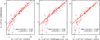 |
Fig. 6. X-ray absorption compared with hydrogen density column estimates toward CHEX-MATE galaxy clusters. Left panel: neutral atomic hydrogen density column derived from the HI4PI survey. Middle panel: total hydrogen density column estimated using the method of Willingale et al. (2013). Right panel: total hydrogen density column estimated in this work using the Planck and HI4PI surveys. XMM-Newton measurements are jointly fitted with projected temperature and metallicity of the intra-cluster gas in an annular region delimited by a cluster-centric radius range of [0.15, 0.6]×r500. The red (black) data points indicate X-ray measurements achieved with an S/N higher (lower) than 2. The red curves depict a linear regression through red points. The labels in the lower right corner of each plot indicate the median, Med(ΔNH/NH), and standard deviation, σ(ΔNH/NH), of the relative differences separating both coordinates of each red point. The dash-dotted lines indicate the identity line that is most similar to the best-fit line in the right panel. |
The impact of the mass fractions of molecular hydrogen provided by the present work on the measurements of CHEX-MATE cluster temperatures is evaluated in Fig. 7. Specifically, average spectroscopic cluster temperatures, kT(NHI) and kT(NH), were extracted assuming the X-ray absorption to be given by the neutral and total hydrogen density columns, respectively. Each kT value was extracted within annular regions delimited by a cluster-centric radius range of [0.15, 0.75]×r500, X, together with characteristic cluster radii, r500, X, gas masses, Mgas, 500, X, and YX mass proxies, YX = Mgas, 500, X × kT. YX and kT values were iteratively reached from convergence of cluster mass estimates, M500, X, following the YX − M500, X scaling relation of Arnaud et al. (2010). The median values of the relative difference separating cluster temperatures measured assuming NH and NHI as the X-ray absorption are 0.1% for clusters of the low NHI category (40% of the CHEX-MATE sample), 1% for cluster of the intermediate NHI category (40% of the CHEX-MATE sample), and 7% for clusters of the high NHI category (20% of the CHEX-MATE sample). As expected for the high Galactic latitudes that are prevalently probed by the CHEX-MATE cluster population, these values suggest that the impact of the mass fractions of molecular hydrogen only becomes significant on temperature measurements of about 20% of the cluster sample located behind the highest NHI regions.
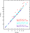 |
Fig. 7. Comparison between temperature measurements performed toward CHEX-MATE clusters assuming X-ray absorptions given by NH and NHI for three intervals of increasing NHI values. The cluster temperatures are jointly fitted with ICM metallicity in an annular region delimited by a cluster-centric radius range of [0.15, 0.75]×r500, X, associated with the YX mass proxy (see details in Sect. 5). |
Infrared Astronomical Satellite.
Cosmic Background Explorer – Far Infrared Absolute Spectrophotometer.
XMM: X-ray Multi Mirror Mission.
Parameters a and b were inferred using IDL function LINFIT as a result of the normal equations of a linear least-squares regression.
The cluster radii result from SZ estimates released as part of the second Planck catalogue of SZ sources (Planck Collaboration XXVII 2016).
Regressions were performed using IDL function MPFIT, which performs a Levenberg–Marquardt χ2 minimisation.
Acknowledgments
We thank and the anonymous referee and Paolo Tozzi for their comments that helped us improve the manuscript. H.B., P.M., F.D.L., and F.O. acknowledge financial contribution from the contracts ASI-INAF Athena 2019-27-HH.0, “Attività di Studio per la comunità scientifica di Astrofisica delle Alte Energie e Fisica Astroparticellare” (Accordo Attuativo ASI-INAF n. 2017-14- H.0), from the European Union’s Horizon 2020 Programme under the AHEAD2020 project (grant agreement n. 871158), support from INFN through the InDark initiative, from “Tor Vergata” Grant “SUPERMASSIVE-Progetti Ricerca Scientifica di Ateneo 2021”, and from Fondazione ICSC, Spoke 3 Astrophysics and Cosmos Observations. National Recovery and Resilience Plan (Piano Nazionale di Ripresa e Resilienza, PNRR) Project ID CN_00000013 ‘Italian Research Center on High-Performance Computing, Big Data and Quantum Computing’ funded by MUR Missione 4 Componente 2 Investimento 1.4: Potenziamento strutture di ricerca e creazione di “campioni nazionali di R&S (M4C2-19 )” – Next Generation EU (NGEU). E.P. acknowledges the support by INSU/CNRS and CNES. Observations presented in this work were obtained with Planck and XMM-Newton, two ESA science missions with instruments and contributions that are directly funded by ESA Member States, NASA, and Canada.
References
- Arnal, E. M., Bajaja, E., Larrarte, J. J., Morras, R., & Pöppel, W. G. L. 2000, A&AS, 142, 35 [NASA ADS] [CrossRef] [EDP Sciences] [Google Scholar]
- Arnaud, M., Pratt, G. W., Piffaretti, R., et al. 2010, A&A, 517, A92 [CrossRef] [EDP Sciences] [Google Scholar]
- Asplund, M., Grevesse, N., Sauval, A. J., & Scott, P. 2009, ARA&A, 47, 481 [NASA ADS] [CrossRef] [Google Scholar]
- Bajaja, E., Arnal, E. M., Larrarte, J. J., et al. 2005, A&A, 440, 767 [NASA ADS] [CrossRef] [EDP Sciences] [Google Scholar]
- Bohlin, R. C., Savage, B. D., & Drake, J. F. 1978, ApJ, 224, 132 [Google Scholar]
- Boulanger, F., & Perault, M. 1988, ApJ, 330, 964 [NASA ADS] [CrossRef] [Google Scholar]
- Boulanger, F., Abergel, A., Bernard, J. P., et al. 1996, A&A, 312, 256 [Google Scholar]
- Bourdin, H., Arnaud, M., Mazzotta, P., et al. 2011, A&A, 527, A21 [NASA ADS] [CrossRef] [EDP Sciences] [Google Scholar]
- CHEX-MATE Collaboration 2021, A&A, 650, A104 [NASA ADS] [CrossRef] [EDP Sciences] [Google Scholar]
- Dame, T. M., Hartmann, D., & Thaddeus, P. 2001, ApJ, 547, 792 [Google Scholar]
- Desert, F. X., Bazell, D., & Boulanger, F. 1988, ApJ, 334, 815 [NASA ADS] [CrossRef] [Google Scholar]
- Fixsen, D. J. 2009, ApJ, 707, 916 [Google Scholar]
- Giard, M., Montier, L., Pointecouteau, E., & Simmat, E. 2008, A&A, 490, 547 [NASA ADS] [CrossRef] [EDP Sciences] [Google Scholar]
- Gillmon, K., Shull, J. M., Tumlinson, J., & Danforth, C. 2006, ApJ, 636, 891 [NASA ADS] [CrossRef] [Google Scholar]
- Hartmann, D., & Burton, W. B. 1997, Atlas of Galactic Neutral Hydrogen (Cambridge: Cambridge University Press) [Google Scholar]
- HI4PI Collaboration (Ben Bekhti, N., et al.) 2016, A&A, 594, A116 [NASA ADS] [CrossRef] [EDP Sciences] [Google Scholar]
- Hurier, G., Macías-Pérez, J. F., & Hildebrandt, S. 2013, A&A, 558, A118 [NASA ADS] [CrossRef] [EDP Sciences] [Google Scholar]
- Kalberla, P. M. W., Burton, W. B., Hartmann, D., et al. 2005, A&A, 440, 775 [NASA ADS] [CrossRef] [EDP Sciences] [Google Scholar]
- Kerp, J., Winkel, B., Ben Bekhti, N., Flöer, L., & Kalberla, P. M. W. 2011, Astron. Nachr., 332, 637 [NASA ADS] [CrossRef] [Google Scholar]
- Lovisari, L., & Reiprich, T. H. 2019, MNRAS, 483, 540 [Google Scholar]
- McClure-Griffiths, N. M., Pisano, D. J., Calabretta, M. R., et al. 2009, ApJS, 181, 398 [NASA ADS] [CrossRef] [Google Scholar]
- Meisner, A. M., & Finkbeiner, D. P. 2015, ApJ, 798, 88 [Google Scholar]
- Montier, L. A., & Giard, M. 2005, A&A, 439, 35 [NASA ADS] [CrossRef] [EDP Sciences] [Google Scholar]
- Planck Collaboration VII. 2014, A&A, 571, A7 [NASA ADS] [CrossRef] [EDP Sciences] [Google Scholar]
- Planck Collaboration XI. 2014, A&A, 571, A11 [NASA ADS] [CrossRef] [EDP Sciences] [Google Scholar]
- Planck Collaboration VIII. 2016, A&A, 594, A8 [NASA ADS] [CrossRef] [EDP Sciences] [Google Scholar]
- Planck Collaboration XXII. 2016, A&A, 594, A22 [NASA ADS] [CrossRef] [EDP Sciences] [Google Scholar]
- Planck Collaboration XXIII. 2016, A&A, 594, A23 [NASA ADS] [CrossRef] [EDP Sciences] [Google Scholar]
- Planck Collaboration XXVII. 2016, A&A, 594, A27 [NASA ADS] [CrossRef] [EDP Sciences] [Google Scholar]
- Planck Collaboration Int. XLIII. 2016, A&A, 596, A104 [NASA ADS] [CrossRef] [EDP Sciences] [Google Scholar]
- Pointecouteau, E., Arnaud, M., Kaastra, J., & de Plaa, J. 2004, A&A, 423, 33 [NASA ADS] [CrossRef] [EDP Sciences] [Google Scholar]
- Rachford, B. L., Snow, T. P., Tumlinson, J., et al. 2002, ApJ, 577, 221 [Google Scholar]
- Rachford, B. L., Snow, T. P., Destree, J. D., et al. 2009, ApJS, 180, 125 [NASA ADS] [CrossRef] [Google Scholar]
- Reach, W. T., Wall, W. F., & Odegard, N. 1998, ApJ, 507, 507 [CrossRef] [Google Scholar]
- Reach, W. T., Heiles, C., & Bernard, J.-P. 2015, ApJ, 811, 118 [NASA ADS] [CrossRef] [Google Scholar]
- Reiprich, T. H., Veronica, A., Pacaud, F., et al. 2021, A&A, 647, A2 [EDP Sciences] [Google Scholar]
- Röhser, T., Kerp, J., Lenz, D., & Winkel, B. 2016, A&A, 596, A94 [NASA ADS] [CrossRef] [EDP Sciences] [Google Scholar]
- Roncarelli, M., Pointecouteau, E., Giard, M., Montier, L., & Pello, R. 2010, A&A, 512, A20 [NASA ADS] [CrossRef] [EDP Sciences] [Google Scholar]
- Savage, B. D., Bohlin, R. C., Drake, J. F., & Budich, W. 1977, ApJ, 216, 291 [NASA ADS] [CrossRef] [Google Scholar]
- Schellenberger, G., Reiprich, T. H., Lovisari, L., Nevalainen, J., & David, L. 2015, A&A, 575, A30 [NASA ADS] [CrossRef] [EDP Sciences] [Google Scholar]
- Smith, R. K., Brickhouse, N. S., Liedahl, D. A., & Raymond, J. C. 2001, ApJ, 556, L91 [Google Scholar]
- Snow, T. P., & McCall, B. J. 2006, ARA&A, 44, 367 [NASA ADS] [CrossRef] [Google Scholar]
- Valdivia, V., Hennebelle, P., Gérin, M., & Lesaffre, P. 2016, A&A, 587, A76 [NASA ADS] [CrossRef] [EDP Sciences] [Google Scholar]
- Verner, D. A., Ferland, G. J., Korista, K. T., & Yakovlev, D. G. 1996, ApJ, 465, 487 [Google Scholar]
- Wakelam, V., Bron, E., Cazaux, S., et al. 2017, Mol. Astrophys., 9, 1 [Google Scholar]
- Willingale, R., Starling, R. L. C., Beardmore, A. P., Tanvir, N. R., & O’Brien, P. T. 2013, MNRAS, 431, 394 [Google Scholar]
- Wilms, J., Allen, A., & McCray, R. 2000, ApJ, 542, 914 [Google Scholar]
Appendix A: Table
Mass fraction of molecular hydrogen (f) and total hydrogen density column (NH) estimates toward CHEX-MATE clusters. f and NH derive from three averaged values of these quantities and associated uncertainties in the intra-cluster radius range [3, 6]×r500.
All Tables
Mass fraction of molecular hydrogen (f) and total hydrogen density column (NH) estimates toward CHEX-MATE clusters. f and NH derive from three averaged values of these quantities and associated uncertainties in the intra-cluster radius range [3, 6]×r500.
All Figures
|
Fig. 1. Calibration of the antenna temperature of the HFI 857 GHz map in NHI units. Left panel: HFI 857 GHz map intensity observable within a dust-gas correlation region, characterised by low NHI values, a low contribution of intermediate- or high-velocity clouds (IVC and HVC) to the NHI values, and a low contamination from thermal SZ sources (see details in Sect. 3). Right panel: pixel-to-pixel correlation and linear regression between the HFI 857 GHz and HI4PI NHI maps in the sky region visible in the left panel. |
| In the text | |
|
Fig. 2. Stacked radial profiles of the SZ signal registered toward CHEX-MATE clusters by the Planck HFI instrument. These profiles radially average HFI frequency maps that were first high-pass filtered and show details of an angular resolution higher than 1 sq. deg. As detailed in Sect. 4, the resulting SZ signal (black points) was corrected for a linear combination of CMB and Galactic thermal dust templates. The dark blue and light blue lines depict the arithmetical mean of CMB and thermal SZ templates that were fit to the data set for each individual cluster, respectively. The red lines depict the individual cluster templates associated with Galactic thermal dust. |
| In the text | |
|
Fig. 3. Stacked radial profiles of the neutral atomic hydrogen density column (NHI, single lines) compared with ISM proxies of the total hydrogen density column (NH, lines with errors) for three intervals of increasing NHI values. NHI profiles radially average patches of the all-sky HI4PI survey. NH proxies, NH ≡ ϕ(I⟨s(857)⟩), are inferred from HFI measurements of the dust emission at 857 GHz, which we corrected for local variations in the dust SED (see also Eqs. (3) and (6)). The shaded areas depict the dispersions of differences between NH and NHI values. The error bars depict the uncertainties on the average values of these differences. |
| In the text | |
|
Fig. 4. Histograms of the thermal dust emission excesses over hydrogen density column, ϕ(I⟨s(857)⟩)/NHI, registered for each CHEX-MATE clusters in the intra-cluster radius range [3, 6]×r500. The vertical lines indicate the median values of the excesses. The lower to upper panels correspond to the three intervals of increasing NHI values that were used to plot stacked radial profiles of I857 and NHI in Fig. 3. |
| In the text | |
|
Fig. 5. Comparison of atomic (black) and total (dark blue) hydrogen density columns derived in this work around individual CHEX-MATE clusters with NH estimates provided by the all-sky modelling of Willingale et al. (2013). |
| In the text | |
|
Fig. 6. X-ray absorption compared with hydrogen density column estimates toward CHEX-MATE galaxy clusters. Left panel: neutral atomic hydrogen density column derived from the HI4PI survey. Middle panel: total hydrogen density column estimated using the method of Willingale et al. (2013). Right panel: total hydrogen density column estimated in this work using the Planck and HI4PI surveys. XMM-Newton measurements are jointly fitted with projected temperature and metallicity of the intra-cluster gas in an annular region delimited by a cluster-centric radius range of [0.15, 0.6]×r500. The red (black) data points indicate X-ray measurements achieved with an S/N higher (lower) than 2. The red curves depict a linear regression through red points. The labels in the lower right corner of each plot indicate the median, Med(ΔNH/NH), and standard deviation, σ(ΔNH/NH), of the relative differences separating both coordinates of each red point. The dash-dotted lines indicate the identity line that is most similar to the best-fit line in the right panel. |
| In the text | |
|
Fig. 7. Comparison between temperature measurements performed toward CHEX-MATE clusters assuming X-ray absorptions given by NH and NHI for three intervals of increasing NHI values. The cluster temperatures are jointly fitted with ICM metallicity in an annular region delimited by a cluster-centric radius range of [0.15, 0.75]×r500, X, associated with the YX mass proxy (see details in Sect. 5). |
| In the text | |
Current usage metrics show cumulative count of Article Views (full-text article views including HTML views, PDF and ePub downloads, according to the available data) and Abstracts Views on Vision4Press platform.
Data correspond to usage on the plateform after 2015. The current usage metrics is available 48-96 hours after online publication and is updated daily on week days.
Initial download of the metrics may take a while.