| Issue |
A&A
Volume 678, October 2023
|
|
|---|---|---|
| Article Number | A44 | |
| Number of page(s) | 17 | |
| Section | Extragalactic astronomy | |
| DOI | https://doi.org/10.1051/0004-6361/202346971 | |
| Published online | 02 October 2023 | |
Reeling in the Whirlpool galaxy: Distance to M 51 clarified through Cepheids and the type IIP supernova 2005cs⋆,⋆⋆
1
Max-Planck-Institute for Astrophysics, Karl-Schwarzschild-Str. 1, 85741 Garching, Germany
e-mail: This email address is being protected from spambots. You need JavaScript enabled to view it.
2
Technical University Munich, TUM Department of Physics, James-Franck-Str. 1, 85741 Garching, Germany
3
École Polytechnique Fédérale de Lausanne (EPFL), Observatoire de Sauverny, Institute of Physics, Laboratory of Astrophysics, 1290 Versoix, Switzerland
4
Exzellenzcluster ORIGINS, Boltzmannstr. 2, 85748 Garching, Germany
5
Aix-Marseille Univ., CNRS, CNES, LAM, 13388 Marseille, France
6
European Southern Observatory, Karl-Schwarzschild-Str. 2, 85741 Garching, Germany
Received:
23
May
2023
Accepted:
23
July
2023
Abstract
Context. The distance to the Whirlpool galaxy, M 51, is still debated, even though the galaxy has been studied in great detail. Current estimates range from 6.02 to 9.09 Mpc, and different methods yield discrepant results. No Cepheid distance has been published for M 51 to date.
Aims. We aim to estimate a more reliable distance to M 51 through two independent methods: Cepheid variables and their period-luminosity relation, and an augmented version of the expanding photosphere method (EPM) on the type IIP supernova SN 2005cs, which exploded in this galaxy.
Methods. For the Cepheid variables, we analysed a recently published Hubble Space Telescope catalogue of stars in M 51. By applying filtering based on the light curve and colour-magnitude diagram, we selected a high-quality sample of M 51 Cepheids to estimate the distance through the period-luminosity relation. For SN 2005cs, an emulator-based spectral fitting technique was applied, which allows for the fast and reliable estimation of the physical parameters of the supernova atmosphere. We augmented the established framework of EPM with these spectral models to obtain a precise distance to M 51.
Results. The two resulting distance estimates are DCep = 7.59 ± 0.30 Mpc and D2005cs = 7.34 ± 0.39 Mpc using the Cepheid period-luminosity relation and the spectral modelling of SN 2005cs, respectively. This is the first published Cepheid distance for this galaxy. The obtained values are precise to 4–5% and are fully consistent within 1σ uncertainties. Because these two estimates are completely independent, they can be combined for an even more precise estimate, which yields DM 51 = 7.50 ± 0.24 Mpc (3.2% uncertainty).
Conclusions. Our distance estimates agree with most of the results obtained previously for M 51, but they are more precise than the earlier counterparts. However, they are significantly lower than the TRGB estimates, which are often adopted for the distance to this galaxy. The results highlight the importance of direct cross-checks between independent distance estimates so that systematic uncertainties can be quantified. Because of the large discrepancy, this finding can also affect distance-sensitive studies and their discussion for objects within M 51, as well as the estimation of the Hubble constant through the type IIP standardizable candle method, for which SN 2005cs is a calibrator object.
Key words: stars: distances / stars: variables: Cepheids / supernovae: individual: SN 2005cs / radiative transfer
The Cepheid catalogue shown in Table B.1 is available at the CDS via anonymous ftp to cdsarc.cds.unistra.fr (130.79.128.5) or via https://cdsarc.cds.unistra.fr/viz-bin/cat/J/A+A/678/A44
The data produced in this work, such as the final M 51 Cepheid catalogue and the flux calibrated spectral time series of SN 2005cs are available at the GitHub page of the author (https://github.com/Csogeza/M51).
© The Authors 2023
 Open Access article, published by EDP Sciences, under the terms of the Creative Commons Attribution License (https://creativecommons.org/licenses/by/4.0), which permits unrestricted use, distribution, and reproduction in any medium, provided the original work is properly cited.
This article is published in open access under the Subscribe to Open model.
Open access funding provided by Max Planck Society.
1. Introduction
The Whirlpool galaxy (or Messier 51, M 51) is one of the best-known extragalactic objects in the sky for professional and amateur astronomers. Despite its proximity and many observations conducted by generations of astronomers, the distance to M 51 remains uncertain compared to other well-studied galaxies, with little agreement between the various methods (see e.g. McQuinn et al. 2016). This uncertainty is a limiting factor for studies that use the distance as an input, such as spatially resolved or luminosity-dependent analyses, for instance in the context of star formation (Heyer et al. 2022), X-ray pulsar brightness (Rodríguez Castillo et al. 2020), or the kinematics of the interstellar medium (Pineda et al. 2020). Moreover, the distance uncertainty for M 51 also affects the extragalactic distance scale because M 51 is one of the few calibrator hosts for the type II supernova standardizable candle method (SCM) through the underluminous type IIP supernova SN 2005cs (de Jaeger et al. 2022).
In recent years, a multitude of methods has been used to constrain the distance to M 51, which yielded results in a wide range of values: the Tully–Fisher method (Tully & Fisher 1977; resulting in distances in the range of 4.9–12.2 Mpc; e.g. Tutui & Sofue 1997), the expanding photosphere method (EPM; Kirshner & Kwan 1974) applied to type II supernovae (6.02–8.40 Mpc; e.g. Takáts & Vinkó 2006; Vinkó et al. 2012), the planetary nebula luminosity function (PNLF; Jacoby 1989; 7.62–8.4 Mpc; Feldmeier et al. 1997; Ciardullo et al. 2002), the surface brightness fluctuation (SBF; Tonry & Schneider 1988; 7.31–7.83 Mpc; e.g. Tonry et al. 2001; Ciardullo et al. 2002), and the tip of the red giant branch (TRGB; Lee et al. 1993; 8.58–9.09 Mpc; Tikhonov et al. 2015; McQuinn et al. 2016), which is most frequently quoted as the distance to M 51 (as discussed in Sect. 6). For a more complete review of these distances and their determination, we refer to McQuinn et al. (2016). Interestingly, no Cepheid distance has been determined for this galaxy to date, despite the large number of observations obtained by the Hubble Space Telescope (HST) in the past decades, for example, based on several supernovae (the type Ic SN 1994I, the low-luminosity type IIP SN 2005cs, and the type IIb SN 2011dh) or with the aim of studying stellar variability (Conroy et al. 2018). In this work, we attempt to obtain a distance to M 51 using two independent techniques: based on Cepheid variables (which is the first dedicated Cepheid study for M 51), and by applying an augmented version of EPM on SN 2005cs.
Cepheids are well-known pulsating variable stars providing one of the most robust and simple distance estimation methods through the Leavitt period-luminosity relation (Leavitt & Pickering 1912), which made these stars the backbone of extragalactic distance measurements and Hubble constant estimations (e.g. Riess et al. 2019, 2022, see Sect. 3.1). On the other hand, type II supernovae also provide a well-established way to determine distances through the EPM (Kirshner & Kwan 1974). This technique provides an independent distance estimation that can be used for galaxies even in the Hubble flow (see Sect. 3.2). As opposed to the Cepheid method, which was not applied to M 51 before, the EPM has been used multiple times in the literature on SN 2005cs to constrain the distance of this galaxy (Takáts & Vinkó 2006; Dessart et al. 2008; Vinkó et al. 2012; Bose & Kumar 2014). However, as we further describe in Sect. 3.2, the method has recently undergone several improvements that increased its accuracy (Vogl et al. 2020). Hence, pairing and comparing the results of this augmented EPM with the first Cepheid-based measurement for M 51 offers an excellent way to narrow down the distance to this galaxy, and it provides two independent distance estimates that can serve to understand the respective systematic uncertainties.
This paper is structured as follows: in Sect. 2 we review the data we adopted for our analysis. In Sect. 3 we introduce and provide a brief outline for the different techniques. In Sect. 4 and Sect. 5 we present the individual steps of the analysis for the Cepheids and SN 2005cs. In Sect. 6 we then discuss these results and summarise our findings.
2. Data
To obtain a Cepheid distance to M 51, we made use of the catalogue and data presented in Conroy et al. (2018, hereafter C18), which were derived based on 34 epochs taken between October 2016 and September 2017 by HST during Cycle 24, using the Advanced Camera for Surveys (ACS). The photometric data published in C18 were derived using the DOLPHOT software package (Dolphin 2000). Although this is a different software from the one that is regularly used for the reduction in Cepheid distance studies (namely DAOPHOT; e.g. Riess et al. 2022), the steps taken for the brightness and error budget estimation (e.g. the point-spread-function (PSF) model estimation or the artificial star tests) match the procedure described in the latest Cepheid works (e.g. Yuan et al. 2022). The applied photometric techniques were also tested before in the context of the Panchromatic Hubble Andromeda Treasury (PHAT) survey (Dalcanton et al. 2012), which showed its high quality. A recent work has also investigated the consistency of the different reduction methods (DAOPHOT and DOLPHOT), finding good agreement (Jang 2023). To ensure the precision of the reduction, C18 adopted the parameter settings from Dalcanton et al. (2012; e.g. the aperture size, the detection threshold, and the maximum step size for positional iteration; for the complete list, see Table 4 in Dalcanton et al. 2012).
The final C18 catalogue consists of F606W and F814W observations at up to 34 epochs for ∼72 000 stars. In addition to presenting the photometry, C18 carried out a Lomb–Scargle method-based analysis for the observations (Lomb 1976; Scargle 1982) with the goal of studying long-term stellar variability in M 51. This analysis showed a period-luminosity relation that indicated that numerous Cepheids were also observed and that the data can be used to determine the distance to M 51. We emphasise that the number of available epochs in this catalogue is significantly higher than what is usually available for extragalactic Cepheids. This makes C18 an exceptionally rich dataset.
To derive the supernova distance, we applied an augmented version of EPM to the data of SN 2005cs. SN 2005cs is a type IIP supernova (SN IIP). It was discovered on 2005 June 28 by Kloehr et al. (2005). It was followed thoroughly both photometrically and spectroscopically (e.g. by Pastorello et al. 2006, 2009). We adopted the photometric data obtained by the Katzman Automatic Imaging Telescope (KAIT; Filippenko et al. 2001) owing to its good coverage and quality, along with early photometric observations from amateur astronomers as collected by Pastorello et al. (2009). We included spectroscopic observations from multiple sources that were taken in the epoch range required for our EPM approach, as described in Sect. 3.2: one spectrum from the Shane telescope1 using KAST2, additional three spectra from the Ekar telescope3 obtained using the AFOSC spectrograph4, one spectrum from the Swift satellite5, one spectrum obtained by TNG6 DOLORES7, and finally, one spectrum obtained by the P200 telescope8 using DBSP9. For more details on the data, we refer to Pastorello et al. (2009).
3. Methods
In this section, we discuss the methods we used to infer the distance to M 51. It is important to note that the methods are completely independent of one another; in particular, the supernova-based method requires no input or calibration from other techniques and acts as a primary distance estimator.
3.1. Cepheid period-luminosity relation
The Cepheid period-luminosity relation (PL relation hereafter; Leavitt & Pickering 1912) is the well-known correlation between the pulsation period and the luminosity of Cepheids. It has been used to determine extragalactic distances for more than a century (Hertzsprung 1913). These distances provide the backbone of precise distance estimations today (Riess et al. 2022). The physical background of this relation and its general usage has been described in detail multiple times in the literature (see e.g. Sandage & Tammann 1968; Madore & Freedman 1991; Freedman et al. 2001; Hoffmann et al. 2016). Although easily applicable because only the brightness and pulsation period of Cepheids need to be measured, a significant limitation of the method is the effect of reddening, which increases the scatter in the PL diagrams. To remedy this, observations are usually taken in at least two separate filters, which are then used to calculate reddening-free magnitudes through the so-called Wesenheit function (Madore 1982),
 (1)
(1)
where mV and mI denote the V- and I-band magnitudes, while RI, V − I = AI/E(V − I) denotes the total-to-selective extinction ratio. The Wesenheit function provides the greatest increase in quality when near-infrared observations are available. These observations are intrinsically less sensitive to the reddening, and make the Wesenheit magnitudes more robust against an incorrectly assumed reddening law. Nevertheless, even the optical two-band Wesenheit indices reduce the effect of reddening significantly. For our work, we employed two Wesenheit functions for the specific HST F555W, F606W, and F814W bands,
 (2)
(2)
and
 (3)
(3)
where the total-to-selective extinction ratios were calculated for RV = 3.3 assuming a Fitzpatrick (1999) reddening law and a typical Cepheid SED following Anderson (2022).
For our analysis, we chose NGC 4258 as the anchor galaxy. Its distance is known to a high precision on a geometric basis (based on a maser; Reid et al. 2019), and it hosts several Cepheids (Yuan et al. 2022). The choice of NGC 4258 was also motivated by the fact that it was observed under similar conditions as M 51: the galaxies are at approximately the same distance and were observed by HST with ACS, although using slightly mismatched filters. Hence their direct comparison allows a differential distance estimation. Since NGC 4258 was observed in F555W and F814W, but not in F606W (which was available for M 51 instead of F555W), we only had to characterise the PL-relation in WF555W, F814W (after the relevant magnitudes were converted for the M 51 sample; see Sect. 4.2). Consequently, the observed M 51 F606W magnitudes and the corresponding Wesenheit function were only used directly for sample selection, as described in Sect. 4.
For the distance estimation, following Riess et al. (2022), the PL relation for M 51 can be written as
![Mathematical equation: $$ \begin{aligned}{[W_{F555W, F814W}]}_i = \alpha \cdot (\log P_i - 1) + \beta + \mu _{0,\mathrm{M\,51}} + \gamma \cdot [\mathrm{O/H} ]_i ,\end{aligned} $$](/articles/aa/full_html/2023/10/aa46971-23/aa46971-23-eq4.gif) (4)
(4)
where i indexes the individual Cepheids in the sample, WF555W, F814W denotes the Wesenheit magnitude, [O/H]i is the metallicity with the usual [O/H] = 12 + log(O/H) definition, P is the period of the Cepheids, and the parameters α, β, and γ define the empirical relation. The parameters α and β can be determined by fitting the PL relation of the anchor galaxy, NGC 4258, by adopting its distance modulus (μ0, NGC 4258 = 29.397 ± 0.032 mag; Reid et al. 2019). For γ, we adopted the value of γ = −0.201 ± 0.071 mag dex−1, corresponding to the F555W and F814W filter set from Breuval et al. (2022). This value is slightly different from but also consistent with the factor used by Riess et al. (2022), ZW = −0.251 ± 0.05, which is applicable for the WH Wesenheit magnitudes. However, given the 0.4 dex average metallicity difference between M 51 and NGC 4258 (Zaritsky & Kennicutt 1994; Yuan et al. 2022), this difference between ZW and γ would only lead to a very small distance offset of 1%. Therefore, the exact choice of the metallicity factor does not affect the final estimate strongly.
3.2. Tailored EPM
To estimate the distance to M 51 based on SN 2005cs, we applied a variant of the tailored expanding photosphere method (tailored EPM hereafter; Dessart & Hillier 2006; Dessart et al. 2008; Vogl et al. 2020). The method itself is an augmented version of the classic EPM, which is a geometric technique relating the photospheric radius of a supernova to its angular diameter (Kirshner & Kwan 1974). Although straightforward, the classical method is prone to several systematics and uncertainties (Jones et al. 2009). As pointed out by Dessart & Hillier (2005), these uncertainties can only be reliably suppressed when the relevant physical parameters for the EPM analysis are estimated through the complete radiative transfer-based modelling of the supernova spectra (which is referred to as tailoring the EPM estimation). We call this augmented version the tailored-EPM analysis, which bears many similarities to the spectral fitting expanding atmosphere method (SEAM) introduced by Baron et al. (2004).
For the required spectral modelling of the supernova, we made use of the spectral emulator developed by Vogl et al. (2020), which is based on radiative transfer models calculated with a modified and type II supernova-specific version of TARDIS (Kerzendorf & Sim 2014; Vogl et al. 2019). The emulator not only significantly reduces the time required for the spectral fitting, but also yields precise estimates of the physical parameters based on maximum likelihood estimation. The background of this spectral fitting method has been thoroughly described in Vogl et al. (2020), while its application and the required calibration steps were summarised in Csörnyei et al. (2023). It has been showcased in Vogl et al. (2020) and Vasylyev et al. (2022), and was also shown to provide internally consistent results for sibling supernovae (i.e. supernovae that exploded in the same galaxy, Csörnyei et al. 2023). For our work, we reapplied the steps detailed in these articles, but we summarise them for completeness in Sect. 5.
For the distance measurement, the photospheric angular diameter of the supernova first has to be estimated for each spectral epoch (Θ = Rph/D, where Rph denotes the radius of the photosphere, and D is the distance measured in Mpc). This estimation was made by minimizing the difference between measured and model apparent magnitudes (mobs and m, respectively) at the given epoch, using Θ as argument,
 (5)
(5)
for all available photometric bands S. To estimate the model apparent magnitudes for each of these bands, the distance modulus formula has to be employed, and the distance has to be replaced by the angular diameter as follows:
![Mathematical equation: $$ \begin{aligned}&m_S = M_S^{\mathrm{ph}}(\Sigma ^{*}) - 5 \log [\Theta (\Sigma ^{*})] + A_S \end{aligned} $$](/articles/aa/full_html/2023/10/aa46971-23/aa46971-23-eq6.gif)
with
 (6)
(6)
Here, Σ* denotes the set of physical parameters corresponding to the best fit,  is the absolute magnitude predicted by the radiative transfer model at the position of the photosphere, and AS denotes the broadband dust extinction in the bandpass. It is important to note that the distance D is the only free parameter that is not directly determined by the spectral fits. With this definition, the best-fitting angular diameter Θ* can be determined for each of the relevant spectral epochs.
Finally, when the ejecta is assumed to be in homologous expansion (Rph = vpht), the distance to the supernova and its time of explosion can be estimated through a Bayesian linear fit to the ratios of the angular diameters and the photospheric velocities (Θ/vph) versus time t. In the fit, we assumed Gaussian uncertainties for Θ/vph of 10% of the measured values for a given colour excess, following Dessart & Hillier (2006), Dessart et al. (2008), and Vogl et al. (2020). We set a flat prior for the distance, and for the time of explosion, we used the normalised histogram of the t0 posterior from a fit to the early light curve as the prior (following Csörnyei et al. 2023). However, instead of applying the standard χ2 based likelihood for the EPM, we used the modified fitting approach from Csörnyei et al. (2023) to take the correlated errors caused by the reddening into account. Essentially, we evaluated the EPM on multiple reddening values with this approach. The values were drawn from the distribution of the single epoch best-fit E(B − V) estimates (see Sect. 5.4 about how these values are obtained). This approach in the end yields a more realistic uncertainty on the EPM distance.
4. Cepheids
In order to obtain a proper understanding of the data presented in C18 and to ensure the good quality of the Cepheid sample, we first reanalysed the catalogue starting from the light curves. This in turn allowed us to filter the dataset in multiple steps instead of applying cuts in the colour-magnitude diagram alone.
4.1. Filtering and sample selection
4.1.1. Period filtering
As a first quality estimation for the sample stars, we inspected the robustness of their period, if any, for the entire C18 catalogue. For this step, we compared the periods from C18 obtained with the Lomb–Scargle method in the F606W and F814W filters with one another and with the equivalent values we obtained using discrete Fourier transformation (DFT; Deeming 1975), for which we employed Period04 (Lenz & Breger 2005). Because the period should be independent of the chosen bandpass or analysis method, it can be used for an initial quality estimation. If any of the four obtained values deviated by more than 1% from the rest, we removed the corresponding star from the sample. Furthermore, additional outliers were removed based on the length of the calculated periods. Even though the C18 sample is extremely rich compared to other extragalactic light-curve samples, it is still reasonably sparse; one datapoint was taken every 10 days on average. This places a limit on the maximal non-aliased frequency that can be estimated using C18 (Nyquist 1928; Eyer & Bartholdi 1999). We thus calculated the Nyquist period for each of the remaining sources (PNyq. ≈ 5 − 10 days) and kept only those for which the estimated period was longer. This single step reduced the sample size from ∼72 000 to merely 950. Figure 1 shows the period-Wesenheit plot for the sample after the period filtering. The plotted Wesenheit values were calculated based on Eq. (3), using the C18 catalogue magnitudes.
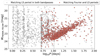 |
Fig. 1. Catalogue PL relation after the filtering based on the Lomb–Scargle (LS) and Fourier periods and the Nyquist frequency. The Wesenheit indices were calculated based on the catalogue magnitudes. The grey dots show the stars for which the LS period matched in the F606W and F814W bands, and the red dots show the stars for which the LS and Fourier periods matched for all filters. |
4.1.2. Filtering the light-curve shapes
After removing non-periodic stars from the catalogue, we attempted to limit our sample further based on their light curves to ensure that only Cepheids or variables with sinusoidal light curves were carried forward. The main reason for this filtering is that light curves more reliably determine the variable type than the colour and brightness. In addition to not being sensitive to reddening, this filtering also removed non-Cepheid stars that seem to scatter into the instability strip region due to reddening or blending. Because most of the sample stars were observed at 34 epochs, which is significantly more than what is available for Cepheids in other galaxies, we were able to perform a more detailed light-curve shape analysis. Instead of inspecting the light curves visually and selecting the Cepheid stars by hand, we applied an automated and reproducible light-curve filtering technique.
We chose to build this step on principal component analysis (PCA; Pearson 1901). The PCA is a commonly used tool for reducing the dimensionality of data, hence allowing for a fast and cheap classification and comparison of dataset elements (see e.g. Dobos et al. 2012; Bhardwaj et al. 2016; Seli et al. 2022). As a reference sample, we adopted the Cepheid set from Yoachim et al. (2009), who applied a PCA to obtain a reliable template set of Cepheid light curves. This set consists of Milky Way and LMC V- and I-band light curves that were covered well enough in phase to allow a detailed analysis of the light-curve shapes. Because the Yoachim et al. (2009) sample of Cepheids was measured in the Bessell system Bessell (1979), we converted the M 51 measurements from the ACS system before the light-curve fitting based on the relations described in Sirianni et al. (2005).
To apply the PCA, we first fit the light curves in the Yoachim et al. (2009) and in the M 51 C18 sample. For this purpose, we applied generalised additive models (GAMs; Hastie & Tibshirani 1990). GAMs are smooth semi-parametric models in the form of a sum of penalised B-splines, which allow modelling non-linear relations with suitable flexibility. The method itself is similar to a Gaussian process fitting that uses splines as the kernel function. This allows a non-parametric, smooth, yet robust fitting method that takes the data uncertainties into account. To implement this method, we made use of the Python package pyGAM (Servén et al. 2018). While the Fourier method would also perform perfectly for Cepheid light curves, it may not handle other types of variables, such as eclipsing binaries, with similar precision. Furthermore, the number of the Fourier components has to be varied from one star to the next in order to avoid overfitting. This can lead to biases when all the light-curve models of different complexities are inspected together, however. Here, GAM models provide a viable alternative because they yield smooth light-curve models whose complexity is automatically set by the data quality. This property makes the technique favourable for generic light curves.
To fit the light curves using GAMs, we first calculated their phase curves using the C18 periods. A comparison of the GAM and DFT fitting is shown in Fig. 2 for a selected few M 51 Cepheids. The two models agree well for good-quality time series. In worse cases, however, in the presence of outliers or larger uncertainties, the naive Fourier method performs worse and increases the model complexity (i.e. overfits the data), as shown in Fig. A.1. However, the GAM model remains smooth and avoids overfitting. It therefore allows for reliable filterings in more uncertain cases as well.
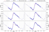 |
Fig. 2. Example of GAM and Fourier fits for a handful M 51 Cepheids. The blue shaded region shows the 95th percentile range of the GAM fits. The plots show that the two models agree perfectly within these uncertainty limits. The grey shaded region shows the extension region for the GAM fitting, which was used to enhance the stability of the phase curve fits towards the edges of the region of interest (close to the phases −0.5 and 0.5). |
This light-curve fitting was carried out for the reference and M 51 sample stars. After this step, each of the light curves was rephased, so that their maximum brightness would fall on the same phase value. We then performed the PCA on the reference sample, obtaining the average curve and the eigenvectors required later on. These vectors are shown in Fig. 3. For our analysis, we used only the first five eigenvectors obtained by the PCA, as they contained > 95% of the variance. This is similar to the choice made by Yoachim et al. (2009), who retained only the first four principal components (although they only aimed to explain ≥90% of the variation).
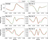 |
Fig. 3. Basis vectors obtained from the PCA applied to the model light curves of the reference sample. The green curves show the Bessell V-band vectors, and the red curves show the I-band vectors. |
The basis was then used to expand the M 51 model phase curves (after applying the same phase normalisation), yielding their expansion coefficients. These expansion coefficients were then used to filter out non-Cepheid variables of the sample. To do this, we set up a grid in the field of expansion coefficients and counted the number of stars that fell in the individual grid elements (i.e. we set up a multi-dimensional histogram for the coefficients). Then, we removed every star for which the expansion coefficients fell in bins that were not covered by the reference sample stars. This approach is similar to defining a convex hull for the reference sample and using this to remove unfit elements with a lower resolution. This step ensured that only Cepheid-like or sinusoidal light curves remained in the sample.
4.1.3. Filtering the colour-magnitude diagram
As a final step of filtering, we removed stars from the sample whose colours were too blue for Cepheids or that were significantly redder than the instability strip (IS). The position of the bluer stars on the colour-magnitude diagram (CMD) cannot be explained by extinction; hence, these stars are either non-Cepheid variables or Cepheids that are strongly blended with clusters (Anderson & Riess 2018). On the other hand, the stars on the redder end can be significantly reddened Cepheids. While the use of the Wesenheit system solves most of the errors tied to the reddening, removing these highly reddened stars will reduce our exposure to the limitations of the Wesenheit relation, resulting in a smaller scatter in the PL relation. To this end, we constructed the cumulative density function (CDF) of the CMD by moving a dividing line along the colour axis. The slope of this dividing line was adopted from Riess et al. (2019) to ensure that it matches the instability strip.
To derive the CDF, we counted the stars left of this dividing line on the CMD, while moving it from bluer colours towards the redder ones. For the bluer edge of the instability strip, we assumed that there is a given offset value for this line at which all stars left of it are outliers, while those to its right are likely Cepheids (see the right plot of Fig. 4). To determine this right offset value, we calculated the first derivative of the CDF. We expect this derivative to initially be flat as long as the dividing line is left of the instability strip on the CMD. In this case, it only moves over a few stars at each step. However, when it enters the instability strip, the number of stars over which the line moves each step would drastically increase. This shows up in the derivative curve as an upturn. Hence, the best position for the dividing line can be set by this upturn. Choosing the offset value corresponding to it will ensure that the filter does not enter the instability strip and thus does not remove bona fide Cepheids while removing as many outliers as possible. A similar scenario was followed at the red edge of the instability strip. Instead of searching for the rise in the CDF derivative, however, we here attempted to determine the offset where it levelled off. This procedure is shown in Fig 4, in which the red lines mark the filter. The best-fit offset value was found to be −0.45 for the blue edge and 0.55 for the red edge in this setup. The plot shows that the resulting Cepheid set aligns well with the reddened theoretical instability strip edges of Anderson et al. (2016; Galactic reddening is applied), and the outliers are properly removed.
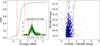 |
Fig. 4. Filtering of the sample stars based on the CMD. Left: CDF of the CMD parametrised by the offset of the adopted IS slope. The inset shows the derivative of the CDF in the range of interest. The dashed red lines show the limits at which the CDF values start to either increase significantly or level off, i.e. the positions of the edges of the M 51 IS. Right: CMD of the M 51 sample, with the IS edge derived based on the CDF (red line). The grey points show the stars that were flagged as outliers. The grey curves show the theoretical instability strip edges from Anderson et al. (2016) reddened by the Galactic colour excess of 0.03 mag for comparison. |
The three filters yielded a sample of M 51 variables that are most likely Cepheids in an almost completely automated manner. In total, the entire catalogue of variable stars was narrowed down from ∼72 000 stars from all types to 638 Cepheids. Table 1 shows the change in the number of sample stars after the individual filters. As a final step, we used the GAM models to recalculate the flux-averaged magnitudes for each of the Cepheids. The magnitude uncertainties were also re-evaluated based on the GAM light-curve fit confidence intervals. The final sample of Cepheids and the corresponding period-luminosity plot are shown in Fig. 5. The plot shows that numerous Cepheids are available for the distance determination, and although the majority of the stars are fundamental-mode Cepheids, the overtone branch is also populated and clearly distinguishable. The positions of the Cepheids in the final sample within M 51 are shown in Fig. 6. The final list of M 51 Cepheids is given in Table B.1.
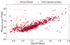 |
Fig. 5. Final set of M 51 Cepheids and their period-luminosity relation. The grey dots show the resulting sample after the first filtering step, and the red points correspond to the final M 51 Cepheid set after the selection for light-curve shape and CMD. |
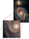 |
Fig. 6. Positions of the final sample of Cepheids within M 51. The background image was taken by the Hubble Space Telescope. The red box indicates the field observed by C18. The yellow shape shows the position and orientation of the M 51 field used for the TRGB by McQuinn et al. (2016). The white cross denotes the position of SN 2005cs. |
Changes in the Cepheid sample size after the individual filtering steps.
4.2. F606W–F555W magnitude conversion
To determine the distance modulus relative to NGC 4258, the F606W observations for the M 51 sample required conversion into F555W. To carry this out, we made use of the spectral library of ATLAS9 stellar atmosphere models (Castelli & Kurucz 2003) that is accessible through pysynphot (STScI Development Team 2013). After limiting the models to the temperature range of Cepheids (5000 K < Teff < 6500 K), we calculated the synthetic F555W − F814W and F606W − F814W colours. Then, by fitting the relation between the colours using a second-order polynomial, we inferred the F555W brightnesses for the M 51 sample. We note that we carried out the conversion into each of the individual measurement epochs instead of just the Cepheid average magnitudes. The conversion curve and its fit are displayed in Fig. 7. The obtained transformation equation is
 (7)
(7)
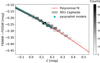 |
Fig. 7. Synthetic pysynphot HST colours and the fitted trend that was subsequently used for the transformation. C denotes the F606W − F814W colour, offset by the sample average. The grey shaded background shows the distribution of the M 51 Cepheid average colours after applying conversion and refitting the light curves. |
where C denotes the original colour, F606W − F814W, with the sample mean subtracted from it (to minimise the fitting and conversion uncertainties). Because our model grid only extended down until 5000 K in temperature, the synthetic data do not cover all colours seen in the catalogue (as some stars scatter up to redder colours due to the reddening). Nevertheless, even for the redder stars, we extrapolated an F555W magnitude using the given transformation curve. From here on, we only used the converted F555W along with the original F814W values for the analysis. Throughout the conversion, no reddening corrections were applied, even though this is known to impose an additional small uncertainty (because the models and the colour conversion assume an extinction-free scenario). On the one hand, constraining this uncertainty properly is hard because it requires knowledge of the internal (within M 51) reddening on a Cepheid-to-Cepheid basis. On the other hand, the good match found between the sample and the slightly reddened theoretical instability strip boundaries (Fig. 4) shows that the majority of the sample is not affected by strong extinction. Assuming a systematic reddening towards the M 51 Cepheids of E(B − V) = 0.03 mag (which is similar to the value found by our analysis of SN 2005cs; see Sect. 5) would only result in a minor F606W − F555W colour difference (smaller than ∼0.01 mag), which is negligible compared to the other systematics affecting our results. Hence, we chose to neglect this term (especially because the highly reddened stars were already clipped using the instability strip boundary estimation presented in Sect. 4.1.3).
4.3. Fitting the period-luminosity relation
In order to measure the distance to M 51 based on the newly found Cepheids, we chose NGC 4258 as the anchor galaxy. It is the only maser host with observed Cepheid variables. We adopted a distance of D = 7.576 ± 0.082 Mpc for NGC 4258 following Reid et al. (2019; which corresponds to a distance modulus of μ = 29.397 ± 0.032 mag). The observed set of Cepheids in NGC 4258, their brightnesses in the HST bands, and their metallicities were adopted from Yuan et al. (2022). The data published in that paper were also obtained using ACS, hence no additional zero-point corrections were necessary. To estimate the reference PL relation fit parameters that were later used for the distance estimation of M 51, we fit Eq. (4) to the NGC 4258 data set. To fit the model, we made use of the UltraNest10 package (Buchner 2021), which allows for Bayesian inference on complex, arbitrarily defined likelihoods based on the nested-sampling Monte Carlo algorithm MLFriends (Buchner 2016, 2019). This allowed us to modify the likelihood. As pointed out for example by Breuval et al. (2022), due to the finite width of the instability strip, the Cepheids exhibit a non-negligible scatter around the true period-luminosity relation, which has to be included in the model. This intrinsic scatter is further enhanced by the photometric uncertainties. To include it, we extended the χ2 likelihood according to Hogg et al. (2010) and applied it in the form
 (8)
(8)
where WVI denotes the observed WF555W, F814W Wesenheit magnitudes, Ω is the set of fit parameters (slope α and offset β of the linear fit), mmodel are the model Wesenheit magnitudes as obtained from the PL relation, and σ2 is the extended uncertainty, defined as the quadrature sum of the measurement uncertainty and the photometric scatter  . We note that
  is defined as a constant for all sample points. It has two components: the unaccounted-for uncertainties, such as the reddening or crowding effects, and the non-negligible width of the instability strip (the intrinsic scatter). For the fitting, we assumed flat priors for all parameters. The resulting maximum a posteriori (MAP) fit along with the derived parameters is shown in Fig. 8.
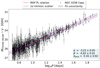 |
Fig. 8. Period-luminosity relation fit to the NGC 4258 anchor data. The red line shows the MAP fit, while the dashed lines denote the range of intrinsic scatter, which is due to observational constraints and the finite width of the instability strip. For simplicity and to reduce scatter, we marginalised over the metallicity values for this plot. |
To estimate the distance of M 51, we applied the result obtained for NGC 4258 by fitting Eq. (4): We fixed the slope of the PL relation to the slope obtained from the reference fit and measured its offset relative to that of the anchor galaxy. We determined the metallicity of each M 51 Cepheid based on its position within the host and by adopting the metallicity gradient obtained by Zaritsky & Kennicutt (1994). According to this, the metallicity of M 51 is 0.4 dex higher on average than that of the anchor galaxy. To determine the distance of M 51 using only NGC 4258 as anchor, we measured the M 51 metallicities relative to those of the NGC 4258 Cepheids. It was therefore not necessary to assume a reference solar value.
Several overtone Cepheids are present in the M 51 set. They can also be used to determine the distance. However, making use of them requires the application of a few changes compared to the regular PL analysis. We therefore conducted two versions of the Cepheid-based distance estimation to M 51: one version without and one version with overtone Cepheids.
4.3.1. Fit of the fundamental mode alone
In the version with the fundamental mode alone, we applied a period cut of 10 days to separate the fundamental-mode Cepheids from their overtone counterparts. The period limit for this cut was motivated by the photometric incompleteness because fundamental-mode Cepheids with shorter periods were too faint and were absent from our sample. Hence, the majority of the removed stars were overtone Cepheids. To fit the PL relation to the filtered dataset, we applied the outlier-rejection method presented in Kodric et al. (2015, 2018). This method works iteratively, and it is based on the median absolute deviation (MAD) of the data points.
Throughout this iterative procedure, the MAD of the dataset is calculated at each step, and then the data point with the greatest deviation is discarded as long as it is at least κ times away from the model value (where κ is a tuning parameter). After this, the MAD is recalculated, and the rejection criterion is re-evaluated. For our work, we adopted κ = 4, in line with the discussion in Kodric et al. (2015). The advantage of the method is that it removes the outliers one by one, which is not only controllable, but is also governed by the statistics of the residuals. No arbitrary cuts therefore have to be made.
The obtained fit for the PL relation of the M 51 Cepheids in this setup is displayed in Fig. 9. To fit the M 51 sample, we recalculated the fit parameters for the anchor galaxy NGC 4258 using only the P > 10 days period range to obtain an unbiased estimate on the slope (although the resulting anchor slope and offset after the step-by-step outlier removal and fitting matched the original values to better than 1%). In this way, we calculated a distance modulus of μM 51 = 29.40 + 0.09 mag and a distance estimate of D = 7.59 ± 0.30 Mpc for M 51.
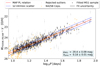 |
Fig. 9. Fitting the PL relation of the fundamental-mode Cepheids in M 51 above the period limit of P > 10 days. The open yellow circles show the NGC 4258 Cepheids for reference, and the faint grey points denote the stars that were rejected by the outlier-detection method. The red line corresponds to the MAP estimate, i.e. the most likely fit. The displayed distance uncertainty includes the systematic terms (namely the uncertainty in the metallicity correction and the reference NGC 4258 PL relation). |
It is worth comparing the fitted observed scatter values: We obtained σphot.,M 51 = 0.20 mag for M 51 and σphot.,N4258 = 0.16 mag for NGC 4258. A similar result of σphot.,M 101 = 0.21 mag can be obtained for M 101 based on the data from Hoffmann et al. (2016). It is important to note that for the comparison NGC 4258 and M 101 values we also used F160W data, which generally reduce the scatter of the Wesenheit magnitudes. The similarity of these values shows the precision of the C18 data and the high quality of the Cepheid sample well.
4.3.2. Fundamental mode and first overtone fit
To investigate how the overtone Cepheids change the distance estimate, we attempted to fit the sample without removing the overtone variables. For this estimation, we assumed that the PL relation slopes of the fundamental mode and overtone Cepheids were the same and that they matched the slopes of the NGC 4258 Cepheid PL relation. This assumption is supported by an earlier study on LMC Cepheids, which showed that the difference between the slopes of the fundamental mode and first overtone Cepheid PL relations is minimal (∼0.12 mag dex−1; see Table 2 in Soszyński et al. 2015). However, it is not known exactly how much brighter the overtone Cepheids should be in the chosen Wesenheit system. For example, Soszyński et al. (2015) found a ∼0.5 mag offset between the PL relations. However, because (a) they used a different Wesenheit system and (b) this offset is not expected to be exactly the same in LMC and M 51, this only allows an approximate estimate for the value in our case. Although the overtone Cepheids can in principle be distinguished from the fundamental mode ones based on light curves, due to their low number they were not separated by the PCA. The analysis of the Fourier components did not separate these two subtypes either because the photometric errors on these Cepheids are relatively high. We thus attempted to separate these two types statistically based on their period-magnitude values.
To do this, we introduced two criteria during the fit. First, we assumed that all stars with P > 10 days were fundamental mode Cepheids because overtone Cepheids of this period are unlikely (Baranowski et al. 2009). For the second criterion, we introduced an offset parameter Δ, which measured the magnitude difference between the fundamental mode and overtone PL relations. Throughout the fitting, each star below the period limit that was at least 1/2 ⋅ Δ magnitudes brighter than the fundamental mode PL relation was assigned to the overtone class. Otherwise, it stayed among the fundamental mode variables. In this way, we were able to fit the PL relation of both modes simultaneously. This ad hoc classification was revised every time a new Δ value was chosen. However, because a Bayesian fitting of this model turned out to be infeasible (due to the simultaneous incorporation of the intrinsic scatter and the offset of overtone Cepheids), we chose not to fit but to marginalise over this offset.
To marginalise, we set up multiple fits assuming different values from a reasonable offset range of [0.45, 0.95] mag. We ran the fitting for all these multiple setups (one of which is shown in Fig. 10), including the previously described outlier rejection, yielding a distance posterior each. Then, we combined these distributions to obtain a marginalised posterior, which included the uncertainty in the offset of the fundamental mode – overtone PL relations.
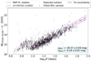 |
Fig. 10. Simultaneous fitting of the fundamental mode and overtone PL relation for the M 51 Cepheid sample. For this run, an offset of 0.75 magnitudes was assumed between the two modes. The red line corresponds to the MAP estimate. The light grey points denote the data points that were rejected by the outlier detection method, and the solid points show the points that were used to fit the relation. As before, the displayed distance uncertainty includes the aforementioned systematic terms. |
Figure 11 shows the combined posterior. By averaging over the combined posterior and then propagating the PL relation fitting and distance modulus uncertainties valid for NGC 4258, we calculated a value of μM 51 = 29.37 ± 0.09 mag (a relative distance modulus of μM 51 − μN4258 = 0.03 ± 0.09 mag), which corresponds to a distance estimate of D = 7.49 ± 0.30 Mpc for M 51. This estimate is consistent with the distance calculated based on the fundamental mode Cepheids alone.
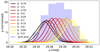 |
Fig. 11. Individual distance posteriors obtained for different offset values Δ (solid curves) and the combined posterior (histogram in the background). |
To cross-check the precision of our NGC 4258-based calibration, we also carried out the distance measurement using Milky Way open cluster Cepheids as an anchor. To do this, we used the recent work of Cruz Reyes & Anderson (2023), in which the period-luminosity relation of Milky Way Cepheids was refined. To perform the calibration, we estimated the α and β fit parameters using equations 26 and 27 presented in Cruz Reyes & Anderson (2023) and based on the pivot wavelengths of the relevant F555W and F814W bands11. The resulting calibration parameters read α = −3.471 and β = −5.998 (the latter of which contains the metallicity term, γ⋅[O/H]MW, Cep ∼ −1.76). To account for the metallicity difference, we measured the [O/H] values relative to that of the Milky Way Cepheid sample when fitting Eq. (4). By carrying out the same distance measurement procedure as above, we arrived at distances of μ = 29.45 ± 0.12 mag and μ = 29.43 ± 0.12 mag for the versions with the fundamental mode alone and the fundamental mode plus first overtone, respectively, which perfectly agree with the results obtained previously. This validates our NGC 4258-based calibration well.
5. SN 2005cs
SN 2005cs is one of the best-known SNe IIP in the literature, mostly because it belongs to the subclass of peculiar underluminous objects (Pastorello et al. 2009; Kozyreva et al. 2022). Because the host is a target that is frequently observed by amateur astronomers, several non-detections were available before its explosion, the latest one just a day before the first detection. The photometric and spectroscopic observations of this supernova are extensively described in Pastorello et al. (2009). The data we adopted and used for this supernova are summarised in Sect. 2. The time series of this supernova was analysed several times with the purpose of obtaining a distance to it based on the standardizable candle method (Hamuy 2005) and the expanding photosphere method (Takáts & Vinkó 2006, 2012; Dessart et al. 2008; Vinkó et al. 2012). The latest independent EPM analysis by Vinkó et al. (2012) yielded a distance of 8.4 ± 0.7 Mpc based on photospheric velocity measurements using model spectra generated by SYNOW (Parrent et al. 2010).
We repeated the analysis based on tailored EPM of SN 2005cs using the spectral emulator introduced in Vogl et al. (2020). The main goal of reanalysing the data of SN 2005cs was twofold: On the one hand, we aimed to investigate how the improvements of the spectral fitting method affect the outcome of the analysis, and on the other hand, we wished to compare this updated result to the independently obtained Cepheid distance. We stress that we did not aim to calibrate the SN II method based on this Cepheid distance because the EPM does not require any such calibration. We instead performed a single-object consistency test for the two methods. The EPM we used was already applied before on SN 2005cs in Vogl et al. (2020). We here discuss the extended version of this analysis (which includes a more complete constraint for the time of explosion, the calibration of spectra to contemporaneous photometry, and the more advanced treatment of reddening in the EPM regression). These improvements have been discussed in detail in Csörnyei et al. (2023).
5.1. Time of explosion
Estimating a high-quality distance to a supernova based on the expanding photosphere method requires precise knowledge of the time of explosion. This parameter is often determined as the mid-point between the first detection and the last non-detection, with an assumed uncertainty of half of the time elapsed between the two. However, this does not make use of all available information, such as the rise of the light curve. When this is taken into account, the EPM results can be improved by constraining the time of explosion with higher precision. Henceforth, we determined the time of explosion based on fitting the early light curve by an inverse exponential following the reasoning of Ofek et al. (2014) and Rubin et al. (2016). We fitted the flux f in band W with a model
![Mathematical equation: $$ \begin{aligned} f_W(t) = f_{m, W} \left[1 - \exp {\left(-\frac{t-t_0}{t_{e, W}}\right)}\right], \end{aligned} $$](/articles/aa/full_html/2023/10/aa46971-23/aa46971-23-eq13.gif) (9)
(9)
where t is the time, t0 is the time of explosion, fm, w is the peak flux, and te, W is the characteristic rise time in the particular band. We carried out this fitting for multiple photometric bands simultaneously to increase the accuracy of the method. Similarly, as in Csörnyei et al. (2023), t0 was treated as a global parameter for the fitting (i.e. it was the same for all bands), while each of the different bands had their own fm, W and te, W parameters. We imposed the additional constraint on the joint fit that the characteristic rise time should increase with wavelength as seen in well-observed SNe before (see e.g. González-Gaitán et al. 2015).
Because SN 2005cs was observed very early on owing to the regular amateur observations of M 51 (see Pastorello et al. 2009 for a list of these observations, some of which are very well described12), the time of explosion can be very tightly constrained through the exponential fitting. The fitting that included the amateur data yielded a precise t0 estimate of JD  (see Fig. 12). This estimate was then used as an independent prior for the EPM regression.
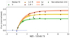 |
Fig. 12. Exponential fit to the light curves of SN 2005cs, including the amateur observations. The shaded regions denote the 68% and 95% confidence intervals. |
5.2. Interpolated light curves
To measure the distance to SN 2005cs, we require knowledge of the absolute and observed magnitudes at matching epochs, which are then compared through Eqs. (5) and (6). Determining the former requires the modelling of spectral observations, but photometry is rarely available simultaneously with spectral epochs. We calculated the observed magnitudes at these epochs by reconstructing the light curves using Gaussian processes (GPs). For the implementation, we used the george13 Python package (Ambikasaran et al. 2015). GPs present an excellent way to interpolate light curves because they provide a non-parametric way of fitting while taking into account the uncertainties in the data. As a result, we obtained smooth and continuous light-curve fits (see Fig. 13) that were used to estimate the brightness in the spectral epochs. The interpolated magnitudes are listed in Table 2.
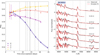 |
Fig. 13. Results of modelling the photometric and spectral time series of SN 2005cs. Left: Gaussian process light-curve fits for 2005cs in the various bands. The dashed grey lines denote the epochs at which a spectrum was taken that was included in our sample. The epochs were measured with respect to MJD 53548.73. Right: the spectra and their emulator fits for the various epochs for an assumed reddening of E(B − V) = 0.03 mag. The grey bands indicate the telluric regions and the sodium band that were masked for the fitting. |
Interpolated magnitudes for SN 2005cs.
5.3. Flux calibration of the spectra
Determining the absolute magnitudes for EPM requires estimating the physical parameters of the supernova, which are best determined through spectral fitting. Because the emulator-based modelling and hence the tailored-EPM analysis requires well-calibrated spectral time series (which is also a requirement for the precise determination of the extinction), the individual spectra had to be recalibrated first based on the photometry. We calculated the relevant set of synthetic magnitudes using the response curves from Bessell & Murphy (2012) and compared them to the corresponding interpolated magnitudes. To correct for flux calibration differences that can be approximated as linear in wavelength, we fitted the first-order trend present in the pairwise ratios of synthetic and interpolated magnitudes against the effective wavelengths of the passbands (including uncertainty inflation following the description of Hogg et al. 2010). We then corrected the spectra for this trend.
5.4. Spectral modelling and tailored EPM
To fit the individual recalibrated spectra, we applied the method from Vogl et al. (2020) and passed the spectral time series to the emulator. This emulator allows for a fast and reliable interpolation of simulated spectra for a given set of physical parameters. The parameter space of the training sets we used for the emulator is summarised in Table 3. These training sets are identical to those used in Csörnyei et al. (2023). Similarly to that work, the choice of the training set used for the emulator was based on the epoch of the spectrum: normally, the first set would be used for spectra younger than 16 days, and the second set for older ones. However, because the evolution of SN 2005cs is accelerated, the training set designed for modelling primarily older spectra had to be employed already at an epoch of 10 days.
Parameter range covered by the extended spectral emulator.
The epoch t of each spectrum was fixed. While the physical parameters were directly estimated by the emulator, we treated the reddening separately: as in Csörnyei et al. (2023), we set up a grid of possible E(B − V) values and performed the maximum likelihood fitting for each of them by reddening the synthetic spectra with the given value. For the lower limit of the E(B − V) grid, we assumed the Galactic colour excess towards the supernova, which was determined based on the dust map of Schlafly & Finkbeiner (2011). The best-fit E(B − V) was then chosen as the average of the E(B − V) values that resulted in the lowest χ2 for the individual spectra.
Because SN 2005cs was a low-luminosity supernova, its spectral evolution was accelerated compared to that of other normal type IIP supernovae (Pastorello et al. 2009). It reached the limits of the emulator faster because of this and because the temperatures were lower. We were therefore only able to use spectra from the first 20 days for the tailored EPM. The recalibrated spectral sequence of SN 2005cs and the corresponding models for the best-fit reddening are shown in Fig. 13. The best-fit parameters for the individual epochs are summarised in Table 4, along with the previous results from Vogl et al. (2020). The fits favoured minimum reddening, and we therefore adopted the reddening of E(B − V) = 0.03 mag obtained by Schlafly & Finkbeiner (2011) towards M 51. This is similar to the estimate that can be obtained from the NaID features seen in the spectra of the sibling supernova, SN 2011dh (Vinkó et al. 2012), hence it is unlikely that the foreground extinction towards M 51 is higher. Moreover, our best-fit extinction estimate is consistent with the value found by previous studies of the spectra of SN 2005cs (Baron et al. 2007; Dessart et al. 2008).
Inferred physical parameters for SN 2005cs.
In general, we find that the obtained Θ/v estimates agree well with the previous values of Dessart et al. (2008). We note that Dessart et al. (2008) modelled two earlier epochs of SN 2005cs as well (at epochs of 4 and 5 days), but they pointed out that the emission line profiles could not be adequately reproduced. When we modelled these epochs, we encountered similar issues and found the estimated physical parameters to be unreliable. Due to these shortcomings, we decided not to include these epochs in the analysis.
As a final step of the distance determination, we performed the EPM analysis of SN 2005cs by fitting a linear function to the Θ/vph(t) values using UltraNest. We performed two fits with different priors on the time of explosion. For the first version, we picked a uniform prior in the range of [−1.3, 2.5] days around the assumed t0 value that was set by the last non-detection (0.5 day before the non-detection, to remain conservative) and the first KAIT detection. For the second fit, we set the prior based on the fit shown in Fig. 12. For both fits, the prior on the distance was set to be flat. To include the systematic uncertainties caused by the reddening in the final error estimate, we applied the treatment described in Csörnyei et al. (2023) for both versions.
The results of the two EPM regressions are shown in Fig. 14. In the more conservative case, we obtain a distance of D = 6.92 ± 0.69 Mpc when the amateur observations are not taken into account. This corresponds to μ = 29.20 ± 0.20 mag. When we tighten the t0 prior used for the EPM regression based on the light curve, the final fit yields a distance of D = 7.34 ± 0.39 Mpc (i.e. μ = 29.33 ± 0.11 mag). We point out that the resulting t0 estimate of the conservative version is in tension with the amateur photometric data because SN 2005cs was already visible in images taken earlier. Hence, we strongly favour the approach that uses the early light-curve fit. We also note that including the tighter constraints reduces the EPM distance uncertainties by almost a factor of two. This highlights the importance of having an informed prior on the time of explosion for a precise distance estimate.
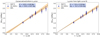 |
Fig. 14. EPM regression obtained for SN 2005cs in the two versions (the left plot shows the more conservative approach, where we adopted a flat prior for t0, and the right plot shows the fit for the t0 prior that is informed by the light curve). The x-axis shows the time elapsed since the explosion epoch t0, MJD 53548.73, for both plots. The points show the evolution of Θ/vph for this supernova as inferred from spectral fitting. The shaded region shows the uncertainty of the fit. |
6. Discussion
We measured two independent distances for M 51: D = 7.59 ± 0.30 Mpc based on Cepheid variables and the period-luminosity relation (by including fundamental mode Cepheids alone, otherwise, this modifies to D = 7.49 ± 0.30 Mpc when using both fundamental mode and first overtone Cepheids and applying the alternative fitting), and D = 7.34 ± 0.39 Mpc based on the updated EPM modelling of SN 2005cs (D = 6.92 ± 0.69 Mpc in the case of the more conservative approach). This consistency highlights the precision of the tailored EPM along with its robustness, and it strengthens the Cepheid distance as well. Because the estimates based on Cepheids and SN 2005cs are completely independent, their average can be taken to obtain a higher-precision distance. When the distance based on the fundamental mode Cepheid alone is combined with the favoured SN 2005cs estimate, the resulting value is D = 7.50 ± 0.24 Mpc. This estimate is precise to 3.2%, which is remarkable for an extragalactic distance. As we expand on below, this distance is more than 10% lower than the estimates used previously for this galaxy (see Table 5).
Previous distance measurements for M 51 from the literature, along with the new estimates.
It is important to note for the Cepheid distances that we did not consider the effects of the stellar association bias in our analysis (i.e. Cepheids may be blended with their birth clusters, which would cause a bias in the estimated brightness). The effect of this bias on the estimated distances was investigated by Anderson & Riess (2018) and will be further inspected by Spetsieri et al. (in prep.). Based on their results, accounting for the bias can have sub-percent effects on the Cepheid brightnesses, and it might increase the inferred distance by the same amount (on the scale of 10−3 mag, as noted in Anderson & Riess 2018). We note that if we accounted for this bias, our Cepheid distance would match the supernova-based result slightly less well, but they would still remain fully consistent.
Figure 15 shows the comparison of our distances with other previous distance estimates. Because we estimated the first Cepheid-based distance to M 51, there are no other results of the same method to which we can compare our value. By comparing our SN 2005cs distance to the other SN II-based distances, we find that it is lower but not inconsistent with the previous EPM and global fitting estimates of Pejcha & Prieto (2015) and Vogl et al. (2020; D = 7.80 ± 0.37 and D = 7.80 ± 0.43, respectively). Most of the difference between our results and theirs can be attributed to the different choices of the explosion time. Compared to the work presented in Vogl et al. (2020), we applied a linear flux correction to the spectra, estimated the time of explosion based on light-curve fits, used an extended set of model spectra for the emulator, and calculated the distance based on a different set of observed spectra. The tentative consistency of our EPM distance with this previous estimate shows that the uncertainties are realistic, that is, the estimator is robust, despite the multiple changes made in the analysis. On the other hand, our EPM distance estimate disagrees with that calculated by Dessart et al. (2008). We found that a significant portion of the mismatch can be explained by the 2.1-day difference in the adopted time of explosion. We note that the t0 estimate of Dessart et al. (2008), which is purely based on the EPM regression, is in tension with the last photometric non-detection of SN 2005cs. If we accounted for this time difference by fixing the time of explosion to the value obtained by Dessart et al. (2008), the two results would be consistent.
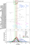 |
Fig. 15. Comparison of the various distance estimates. Top: individual distance estimates from multiple publications making use of the SBF, the TRGB, or optical supernova observations. The coloured regions in the background show the 1σ ranges of the estimates presented in this paper. Bottom: individual distance probability distributions assuming Gaussian uncertainties. |
The most relevant feature in Fig. 15 is the fact that the two distances obtained by us disagree by 2σ at least with the TRGB values, even with the most recently obtained value from McQuinn et al. (2017; D = 8.58 ± 0.44 Mpc, updated from McQuinn et al. 2016 to include systematic uncertainties). The difference between the distance estimates can be even more than 10%, inducing a ∼0.2 − 0.4 mag difference in the absolute magnitudes (15 − 30% difference in flux). Since TRGB distances were used widely as a benchmark for studies that considered the absolute luminosities of objects within M 51 (e.g. supergiant, Jencson et al. 2022, or pulsar studies, Brightman et al. 2022), this difference in distance or luminosity affects the astrophysical results. It also causes a non-negligible change in the SNe IIP standardizable candle method as well, which uses SN 2005cs as a calibrator (de Jaeger et al. 2022). When the TRGB value is used, this object falls slightly away from the rest of the sample in terms of the calibrated absolute magnitude (see Fig. 1 of de Jaeger et al. 2022). The newly estimated Cepheid distance, however, would place SN 2005cs closer to the rest of the sample, which in turn would revise the calibration parameters as well.
An explanation for this offset between the TRGB and the Cepheid (or the EPM-based) distance eludes us. It cannot be ruled out that the offset is due to inherent systematic differences: for example, Anand et al. (2022) found an offset between the TRGB and the maser distance of NGC 4258, our anchor. However, the scale of this offset was only a few percent, hence it cannot explain the entirety of the difference we found. There were also indications of offsets between Cepheid and TRGB distances, and consequently, of the inferred Hubble constants, namely that the TRGB value of Freedman (2021; 69.8 ± 2.2 km s−1) was found to be significantly different from the SH0ES estimate (73.04 ± 1.04 km s−1, Riess et al. 2022). The question whether there truly is a systematic difference may be solved by acquiring a large enough sample of galaxies where both methods to be used for a precision distance estimation (see the HST proposal of Jang et al. 2022).
Another explanation for the offset may be that previous TRGB results overestimated the distance of M 51. As discussed by Jang et al. (2021), Freedman (2021), Anderson (2022), and Madore et al. (2023), the choice of the field (e.g. if it is too close to the disk of the galaxy) can influence the analysis through the internal reddening of the host, or through blending. Moreover, Wu et al. (2023) and Scolnic et al. (2023) have shown that the apparent magnitude of the TRGB feature depends on the contrast between RGB and AGB stars near the tip. This may be important for the McQuinn et al. (2016) TRGB value because the field chosen for analysis lies close to or partially even on top of a spiral arm of M 51. This means that the field is far more crowded and reddened and has a higher contribution from AGB stars than in usual TRGB analyses. This effect was discussed by Anderson et al. (2023) as well. They noted that disk fields could sample a different population of stars than those used to calibrate the TRGB method, and they showed that different groups of stars can exhibit the TRGB at systematically different luminosities. On the other hand, Tikhonov et al. (2015) calculated a distance that was consistent with the estimate of McQuinn et al. (2016), even though the underlying field was farther away from M 51 (but Tikhonov et al. 2015 used one of the earlier versions of the TRGB method; Table 5).
The method for determining the tip of the red giant branch on the CMD has been shown to influence the measurement, as shown by Wu et al. (2023). Curiously, most of the inconsistency between our distances and the TRGB can be remedied when the absolute magnitude of the tip is assumed to be dimmer. Recent analyses (e.g. Jang et al. 2021; Anand et al. 2022) assumed an absolute magnitude of about MF814W = −4.06 mag (similarly to McQuinn et al. 2016). However, assuming a value of MF814W = −3.94 mag, which is perfectly within the range of absolute magnitudes found by Rizzi et al. (2007), would lead to a TRGB distance estimate of μ = 29.55 mag. This is also supported by the recent analysis of Anderson et al. (2023), who found a similarly fainter calibration magnitude for the TRGB method. This would be consistent with our estimates within 2σ. As noted by Rizzi et al. (2007), the TRGB absolute magnitude weakly correlates with the metallicity even in the I band, which could explain the distance offsets, given the supersolar value for M 51.
It is worth noting that despite the large offsets between our estimates and the TRGB value, the Cepheid and EPM distances are consistent with results of secondary distance indicators, such as PNLF (7.62 ± 0.42 Mpc; Ciardullo et al. 2002) and SBF (7.31 ± 0.47 Mpc; Tully et al. 2013). These methods were calibrated based on Cepheids, and a good agreement is therefore expected (nevertheless, it is important that our estimates are independent of these because M 51 had no published Cepheid distance before our analysis, and the supernova distance requires no calibration). Based on these results and the good agreement among all independent indicators except for the TRGB, we find it more likely that M 51 is located closer to us than previously assumed.
7. Conclusions
The distance to M 51 was measured using two independent approaches: the well-established PL relation method of Cepheid variable stars, yielding a distance of D = 7.59 ± 0.30 Mpc (D = 7.49 ± 0.30 Mpc when both fundamental mode and overtone Cepheids are used), and by applying the tailored expanding photosphere method on SN 2005cs, resulting in D = 7.34 ± 0.39 Mpc (D = 6.92 ± 0.69 without using light curve information to estimate the explosion time). Combinination of these two independent estimates yields a distance of DM 51 = 7.50 ± 0.24 Mpc for M 51. The consistency of the obtained values demonstrates the potential of SN IIP-based distances well: Even though the analysis does not rely on any calibration with other distance estimation methods, it produced a distance that is not only comparable in precision but also agrees with the result based on the Cepheid PL relation. A similar consistency was achieved between our results and some other secondary distance indicators, such as surface brightness fluctuations or the planetary nebula luminosity function.
Both of our estimates disagree with the previously obtained TRGB values. It is unclear whether this inconsistency is an inherent difference between the various methods, even though former studies did not show systematic offsets of such magnitudes. Understanding this offset is important from the point of view of luminosity-critical studies: Because the difference between the newly obtained distances and the latest TRGB value is as large as 10%, the choice of the distance measure can significantly affect the astrophysical conclusions for objects within M 51.
This work also demonstrates that the improvements in the spectral modelling have placed non-computation intensive and accurate type IIP supernova distances well within reach. By obtaining spectral time series that are well suited for this type of analysis, these supernovae might be used to estimate distances that are well within the Hubble flow independently of the distance ladder. Data like this have been obtained by the Nearby Supernova Factory and the adh0cc collaborations, with the ultimate goal of inferring the local Universe Hubble constant through tailored EPM.
Shane is the 3 m Donald Shane Telescope, Lick Observatory, California (US).
Kast spectrograph.
Ekar is the 1.82 m Copernico Telescope, INAF, Osservatorio di Asiago, Mt Ekar, Asiago (Italy).
Asiago Faint Object Spectrograph and Camera.
Neil Gehrels Swift Observatory, NASA.
TNG is the 3.5 m Telescopio Nazionale Galileo, Fundacións Galileo Galilei, INAF, Fundación Canaria, La Palma (Canary Islands, Spain).
Device Optimized for the LOw RESolution.
P200 is the Palomar 200-inch Hale Telescope, Palomar Observatory, Caltech, Palomar Mountain, California (US).
Double Spectrograph.
Acknowledgments
The authors thank the anonymous referee for the constructive comments and remarks that helped improve the paper. We also thank Jason Spyromilio for the comments he provided while writing the manuscript, and Zoi Spetsieri for carrying out a check on stellar association bias for the Cepheid sample. The research was completed with the extensive use of Python, along with the numpy (Harris et al. 2020), scipy (Virtanen et al. 2020) and astropy (Astropy Collaboration 2018) modules. This research made use of TARDIS, a community-developed software package for spectral synthesis in supernovae (Kerzendorf & Sim 2014; Kerzendorf et al. 2022). The development of TARDIS received support from the Google Summer of Code initiative and from ESA’s Summer of Code in Space program. TARDIS makes extensive use of Astropy and PyNE. C.V. and W.H. were supported for part of this work by the Excellence Cluster ORIGINS, which is funded by the Deutsche Forschungsgemeinschaft (DFG, German Research Foundation) under Germany’s Excellence Strategy-EXC-2094-390783311. R.I.A. acknowledges support from the European Research Council (ERC) under the European Union’s Horizon 2020 research and innovation programme (Grant Agreement No. 947660). R.I.A. further acknowledges funding by the Swiss National Science Foundation through an Eccellenza Professorial Fellowship (award PCEFP2_194638). S.T. acknowledges funding from the European Research Council (ERC) under the European Union’s Horizon 2020 research and innovation program (LENSNOVA: grant agreement No 771776). S.B. acknowledges support from the Alexander von Humboldt foundation and thanks Sherry Suyu and her group at the Technische Universität München (TUM) for their hospitality. This work was supported by the ‘Programme National de Physique Stellaire’ (PNPS) of CNRS/INSU co-funded by CEA and CNES. The data underlying this work are publicly available (via Wiserep for the Pastorello et al. 2009 data, and via CDS for the Conroy et al. 2018 catalogue).
References
- Ambikasaran, S., Foreman-Mackey, D., Greengard, L., Hogg, D. W., & O’Neil, M. 2015, IEEE Trans. Pattern Anal. Mach. Intel., 38, 252 [Google Scholar]
- Anand, G. S., Tully, R. B., Rizzi, L., Riess, A. G., & Yuan, W. 2022, ApJ, 932, 15 [NASA ADS] [CrossRef] [Google Scholar]
- Anderson, R. I. 2022, A&A, 658, A148 [NASA ADS] [CrossRef] [EDP Sciences] [Google Scholar]
- Anderson, R. I., & Riess, A. G. 2018, ApJ, 861, 36 [NASA ADS] [CrossRef] [Google Scholar]
- Anderson, R. I., Saio, H., Ekström, S., Georgy, C., & Meynet, G. 2016, A&A, 591, A8 [NASA ADS] [CrossRef] [EDP Sciences] [Google Scholar]
- Anderson, R. I., Koblischke, N. W., & Eyer, L. 2023, Nature, submitted [arXiv:2303.04790] [Google Scholar]
- Astropy Collaboration (Price-Whelan, A. M., et al.) 2018, AJ, 156, 123 [Google Scholar]
- Baranowski, R., Smolec, R., Dimitrov, W., et al. 2009, MNRAS, 396, 2194 [NASA ADS] [CrossRef] [Google Scholar]
- Baron, E., Hauschildt, P. H., Branch, D., Kirshner, R. P., & Filippenko, A. V. 1996, MNRAS, 279, 799 [NASA ADS] [CrossRef] [Google Scholar]
- Baron, E., Nugent, P. E., Branch, D., & Hauschildt, P. H. 2004, ApJ, 616, L91 [NASA ADS] [CrossRef] [Google Scholar]
- Baron, E., Branch, D., & Hauschildt, P. H. 2007, ApJ, 662, 1148 [NASA ADS] [CrossRef] [Google Scholar]
- Bessell, M. S. 1979, PASP, 91, 589 [Google Scholar]
- Bessell, M., & Murphy, S. 2012, PASP, 124, 140 [NASA ADS] [CrossRef] [Google Scholar]
- Bhardwaj, A., Kanbur, S. M., Marconi, M., et al. 2016, MNRAS, 466, 2805 [Google Scholar]
- Bose, S., & Kumar, B. 2014, ApJ, 782, 98 [NASA ADS] [CrossRef] [Google Scholar]
- Breuval, L., Riess, A. G., Kervella, P., Anderson, R. I., & Romaniello, M. 2022, ApJ, 939, 89 [NASA ADS] [CrossRef] [Google Scholar]
- Brightman, M., Bachetti, M., Earnshaw, H., et al. 2022, ApJ, 925, 18 [NASA ADS] [CrossRef] [Google Scholar]
- Buchner, J. 2016, Stat. Comput., 26, 383 [Google Scholar]
- Buchner, J. 2019, PASP, 131, 108005 [Google Scholar]
- Buchner, J. 2021, J. Open Source Softw., 6, 3001 [CrossRef] [Google Scholar]
- Castelli, F., & Kurucz, R. L. 2003, IAU Symp., 210, A20 [Google Scholar]
- Ciardullo, R., Feldmeier, J. J., Jacoby, G. H., et al. 2002, ApJ, 577, 31 [Google Scholar]
- Conroy, C., Strader, J., van Dokkum, P., et al. 2018, ApJ, 864, 111 [NASA ADS] [CrossRef] [Google Scholar]
- Cruz Reyes, M., & Anderson, R. I. 2023, A&A, 672, A85 [NASA ADS] [CrossRef] [EDP Sciences] [Google Scholar]
- Csörnyei, G., Vogl, C., Taubenberger, S., et al. 2023, A&A, 672, A129 [NASA ADS] [CrossRef] [EDP Sciences] [Google Scholar]
- Dalcanton, J. J., Williams, B. F., Lang, D., et al. 2012, ApJS, 200, 18 [Google Scholar]
- Deeming, T. J. 1975, Ap&SS, 36, 137 [Google Scholar]
- de Jaeger, T., Galbany, L., Riess, A. G., et al. 2022, MNRAS, 514, 4620 [NASA ADS] [CrossRef] [Google Scholar]
- Dessart, L., & Hillier, D. J. 2005, A&A, 439, 671 [NASA ADS] [CrossRef] [EDP Sciences] [Google Scholar]
- Dessart, L., & Hillier, D. J. 2006, A&A, 447, 691 [NASA ADS] [CrossRef] [EDP Sciences] [Google Scholar]
- Dessart, L., Blondin, S., Brown, P. J., et al. 2008, ApJ, 675, 644 [NASA ADS] [CrossRef] [Google Scholar]
- Dobos, L., Csabai, I., Yip, C.-W., et al. 2012, MNRAS, 420, 1217 [Google Scholar]
- Dolphin, A. E. 2000, PASP, 112, 1397 [NASA ADS] [CrossRef] [Google Scholar]
- Eyer, L., & Bartholdi, P. 1999, A&AS, 135, 1 [NASA ADS] [CrossRef] [EDP Sciences] [Google Scholar]
- Feldmeier, J. J., Ciardullo, R., & Jacoby, G. H. 1997, ApJ, 479, 231 [NASA ADS] [CrossRef] [Google Scholar]
- Ferrarese, L., Mould, J. R., Kennicutt, R. C., Jr., et al. 2000, ApJ, 529, 745 [Google Scholar]
- Filippenko, A. V., Li, W. D., Treffers, R. R., & Modjaz, M. 2001, ASP Conf. Ser., 246, 121 [NASA ADS] [Google Scholar]
- Fitzpatrick, E. L. 1999, PASP, 111, 63 [Google Scholar]
- Freedman, W. L. 2021, ApJ, 919, 16 [NASA ADS] [CrossRef] [Google Scholar]
- Freedman, W. L., Madore, B. F., Gibson, B. K., et al. 2001, ApJ, 553, 47 [Google Scholar]
- González-Gaitán, S., Tominaga, N., Molina, J., et al. 2015, MNRAS, 451, 2212 [CrossRef] [Google Scholar]
- Hamuy, M. 2005, in IAU Colloq. 192: Cosmic Explosions, On the 10th Anniversary of SN1993J, 99, 535 [NASA ADS] [CrossRef] [Google Scholar]
- Harris, C. R., Millman, K. J., van der Walt, S. J., et al. 2020, Nature, 585, 357 [NASA ADS] [CrossRef] [Google Scholar]
- Hastie, T., & Tibshirani, R. 1990, Generalized Additive Models (Milton Park: Routledge) [Google Scholar]
- Hertzsprung, E. 1913, Astron. Nachr., 196, 201 [NASA ADS] [Google Scholar]
- Heyer, M., Gregg, B., Calzetti, D., et al. 2022, ApJ, 930, 170 [NASA ADS] [CrossRef] [Google Scholar]
- Hoffmann, S. L., Macri, L. M., Riess, A. G., et al. 2016, ApJ, 830, 10 [Google Scholar]
- Hogg, D. W., Bovy, J., & Lang, D. 2010, ArXiv e-prints [arXiv:1008.4686] [Google Scholar]
- Iwamoto, K., Nomoto, K., Höflich, P., et al. 1994, ApJ, 437, L115 [NASA ADS] [CrossRef] [Google Scholar]
- Jacoby, G. H. 1989, ApJ, 339, 39 [NASA ADS] [CrossRef] [Google Scholar]
- Jang, I. S. 2023, MNRAS, 521, 1532 [NASA ADS] [CrossRef] [Google Scholar]
- Jang, I. S., Hoyt, T. J., Beaton, R. L., et al. 2021, ApJ, 906, 125 [NASA ADS] [CrossRef] [Google Scholar]
- Jang, I. S., Dhawan, S., Freedman, W. L., et al. 2022, HST Proposal. Cycle 30, #17079 [Google Scholar]
- Jencson, J. E., Sand, D. J., Andrews, J. E., et al. 2022, ApJ, 930, 81 [NASA ADS] [CrossRef] [Google Scholar]
- Jones, M. I., Hamuy, M., Lira, P., et al. 2009, ApJ, 696, 1176 [NASA ADS] [CrossRef] [Google Scholar]
- Kerzendorf, W. E., & Sim, S. A. 2014, MNRAS, 440, 387 [NASA ADS] [CrossRef] [Google Scholar]
- Kerzendorf, W., Sim, S., Vogl, C., et al. 2022, https://zenodo.org/record/6299948 [Google Scholar]
- Kirshner, R. P., & Kwan, J. 1974, ApJ, 193, 27 [NASA ADS] [CrossRef] [Google Scholar]
- Kloehr, W., Muendlein, R., Li, W., Yamaoka, H., & Itagaki, K. 2005, IAU Circ., 8553, 1 [NASA ADS] [Google Scholar]
- Kodric, M., Riffeser, A., Seitz, S., et al. 2015, ApJ, 799, 144 [NASA ADS] [CrossRef] [Google Scholar]
- Kodric, M., Riffeser, A., Seitz, S., et al. 2018, ApJ, 864, 59 [NASA ADS] [CrossRef] [Google Scholar]
- Kozyreva, A., Janka, H.-T., Kresse, D., Taubenberger, S., & Baklanov, P. 2022, MNRAS, 514, 4173 [CrossRef] [Google Scholar]
- Leavitt, H. S., & Pickering, E. C. 1912, Harvard College Observatory Circular, 173, 1 [Google Scholar]
- Lee, M. G., Freedman, W. L., & Madore, B. F. 1993, ApJ, 417, 553 [Google Scholar]
- Lenz, P., & Breger, M. 2005, Commun. Asteroseismol., 146, 53 [Google Scholar]
- Lomb, N. R. 1976, Ap&SS, 39, 447 [Google Scholar]
- Madore, B. F. 1982, ApJ, 253, 575 [NASA ADS] [CrossRef] [Google Scholar]
- Madore, B. F., & Freedman, W. L. 1991, PASP, 103, 933 [Google Scholar]
- Madore, B. F., Freedman, W. L., Owens, K. A., & Jang, I. S. 2023, AJ, 166, 2 [NASA ADS] [CrossRef] [Google Scholar]
- McQuinn, K. B. W., Skillman, E. D., Dolphin, A. E., Berg, D., & Kennicutt, R. 2016, ApJ, 826, 21 [NASA ADS] [CrossRef] [Google Scholar]
- McQuinn, K. B. W., Skillman, E. D., Dolphin, A. E., Berg, D., & Kennicutt, R. 2017, AJ, 154, 51 [NASA ADS] [CrossRef] [Google Scholar]
- Nyquist, H. 1928, Phys. Rev., 32, 110 [CrossRef] [Google Scholar]
- Ofek, E. O., Arcavi, I., Tal, D., et al. 2014, ApJ, 788, 154 [NASA ADS] [CrossRef] [Google Scholar]
- Parrent, J., Branch, D., & Jeffery, D. 2010, Astrophysics Source Code Library [record ascl:1010.055] [Google Scholar]
- Pastorello, A., Sauer, D., Taubenberger, S., et al. 2006, MNRAS, 370, 1752 [NASA ADS] [CrossRef] [Google Scholar]
- Pastorello, A., Valenti, S., Zampieri, L., et al. 2009, MNRAS, 394, 2266 [Google Scholar]
- Pearson, K. F. 1901, London Edinburgh Dublin Philos. Mag. J. Sci., 2, 559 [CrossRef] [Google Scholar]
- Pejcha, O., & Prieto, J. L. 2015, ApJ, 799, 215 [NASA ADS] [CrossRef] [Google Scholar]
- Pineda, J. L., Stutzki, J., Buchbender, C., et al. 2020, ApJ, 900, 132 [NASA ADS] [CrossRef] [Google Scholar]
- Poznanski, D., Butler, N., Filippenko, A. V., et al. 2009, ApJ, 694, 1067 [NASA ADS] [CrossRef] [Google Scholar]
- Reid, M. J., Pesce, D. W., & Riess, A. G. 2019, ApJ, 886, L27 [Google Scholar]
- Richmond, M. W., van Dyk, S. D., Ho, W., et al. 1996, AJ, 111, 327 [NASA ADS] [CrossRef] [Google Scholar]
- Riess, A. G., Casertano, S., Yuan, W., Macri, L. M., & Scolnic, D. 2019, ApJ, 876, 85 [Google Scholar]
- Riess, A. G., Yuan, W., Macri, L. M., et al. 2022, ApJ, 934, L7 [NASA ADS] [CrossRef] [Google Scholar]
- Rizzi, L., Tully, R. B., Makarov, D., et al. 2007, ApJ, 661, 815 [Google Scholar]
- Rodríguez, Ó., Clocchiatti, A., & Hamuy, M. 2014, AJ, 148, 107 [CrossRef] [Google Scholar]
- Rodríguez Castillo, G. A., Israel, G. L., Belfiore, A., et al. 2020, ApJ, 895, 60 [Google Scholar]
- Rubin, A., Gal-Yam, A., De Cia, A., et al. 2016, ApJ, 820, 33 [NASA ADS] [CrossRef] [Google Scholar]
- Sandage, A., & Tammann, G. A. 1968, ApJ, 151, 531 [NASA ADS] [CrossRef] [Google Scholar]
- Scargle, J. D. 1982, ApJ, 263, 835 [Google Scholar]
- Schlafly, E. F., & Finkbeiner, D. P. 2011, ApJ, 737, 103 [Google Scholar]
- Scolnic, D., Riess, A. G., Wu, J., et al. 2023, ApJ, 954, L31 [NASA ADS] [CrossRef] [Google Scholar]
- Seli, B., Oláh, K., Kriskovics, L., et al. 2022, A&A, 659, A3 [NASA ADS] [CrossRef] [EDP Sciences] [Google Scholar]
- Servén, D., Brummitt, C., & Abedi, H. 2018, https://zenodo.org/record/1476122 [Google Scholar]
- Sirianni, M., Jee, M. J., Benítez, N., et al. 2005, PASP, 117, 1049 [Google Scholar]
- Soszyński, I., Udalski, A., Szymański, M. K., et al. 2015, Acta Astron., 65, 297 [NASA ADS] [Google Scholar]
- STScI Development Team 2013, Astrophysics Source Code Library [record ascl:1303.023] [Google Scholar]
- Takáts, K., & Vinkó, J. 2006, MNRAS, 372, 1735 [CrossRef] [Google Scholar]
- Takáts, K., & Vinkó, J. 2012, MNRAS, 419, 2783 [CrossRef] [Google Scholar]
- Tikhonov, N. A., Lebedev, V. S., & Galazutdinova, O. A. 2015, Astron. Lett., 41, 239 [NASA ADS] [CrossRef] [Google Scholar]
- Tonry, J., & Schneider, D. P. 1988, AJ, 96, 807 [Google Scholar]
- Tonry, J. L., Dressler, A., Blakeslee, J. P., et al. 2001, ApJ, 546, 681 [Google Scholar]
- Tully, R. B., & Fisher, J. R. 1977, A&A, 54, 661 [NASA ADS] [Google Scholar]
- Tully, R. B., Courtois, H. M., Dolphin, A. E., et al. 2013, AJ, 146, 86 [NASA ADS] [CrossRef] [Google Scholar]
- Tutui, Y., & Sofue, Y. 1997, A&A, 326, 915 [NASA ADS] [Google Scholar]
- Vasylyev, S. S., Filippenko, A. V., Vogl, C., et al. 2022, ApJ, 934, 134 [NASA ADS] [CrossRef] [Google Scholar]
- Vinkó, J., Takáts, K., Szalai, T., et al. 2012, A&A, 540, A93 [NASA ADS] [CrossRef] [EDP Sciences] [Google Scholar]
- Virtanen, P., Gommers, R., Oliphant, T. E., et al. 2020, Nat. Methods, 17, 261 [Google Scholar]
- Vogl, C., Sim, S. A., Noebauer, U. M., Kerzendorf, W. E., & Hillebrandt, W. 2019, A&A, 621, A29 [NASA ADS] [CrossRef] [EDP Sciences] [Google Scholar]
- Vogl, C., Kerzendorf, W. E., Sim, S. A., et al. 2020, A&A, 633, A88 [NASA ADS] [CrossRef] [EDP Sciences] [Google Scholar]
- Wu, J., Scolnic, D., Riess, A. G., et al. 2023, ApJ, 954, 87 [NASA ADS] [CrossRef] [Google Scholar]
- Yoachim, P., McCommas, L. P., Dalcanton, J. J., & Williams, B. F. 2009, AJ, 137, 4697 [NASA ADS] [CrossRef] [Google Scholar]
- Yuan, W., Macri, L. M., Riess, A. G., et al. 2022, ApJ, 940, 64 [NASA ADS] [CrossRef] [Google Scholar]
- Zaritsky, D., Kennicutt, Robert C. J., & Huchra, J. P., 1994, ApJ, 420, 87 [NASA ADS] [CrossRef] [Google Scholar]
Appendix A: Examples for differences between the Fourier method and GAM
Fig. A.1 shows examples of light curves for which the Fourier and GAM fits yielded significantly different results. In these cases, the naive Fourier method overfits the data. This can be avoided by limiting the number of Fourier terms used for the fitting for each object individually. However, the GAM method performs well in these cases and results in smooth light curves that can still be compared reasonably well to the rest of the sample. Even though the uncertainties are high, these variable stars were still included for the further filtering steps because of the smooth GAM fits, whereas the Fourier method would have removed them using our approach.
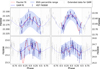 |
Fig. A.1. Example light-curve fits for which the Fourier and the GAM method yield different results. |
Appendix D: Cepheid catalogue
In Tab B.1 we show the list of Cepheids that were found by our filtering. This list is complete, that is, even the stars that were flagged as outliers by the σ clipping method are included. For the full table including photometric errors, we refer to the online version of the article. This table includes all variables that remained in the sample after removing the stars with a bluer colour than the instability strip. The σ clip column shows the variables that were not classified as outliers by the σ clipping algorithm we applied (denoted with the plus). For the full table, we refer to the online appendix of the article or the alternative sources described at the end of the acknowledgements section. The metallicities are measured according to the Zaritsky & Kennicutt (1994) scale.
List of the Cepheid variables found in our analysis.
All Tables
Previous distance measurements for M 51 from the literature, along with the new estimates.
All Figures
|
Fig. 1. Catalogue PL relation after the filtering based on the Lomb–Scargle (LS) and Fourier periods and the Nyquist frequency. The Wesenheit indices were calculated based on the catalogue magnitudes. The grey dots show the stars for which the LS period matched in the F606W and F814W bands, and the red dots show the stars for which the LS and Fourier periods matched for all filters. |
| In the text | |
|
Fig. 2. Example of GAM and Fourier fits for a handful M 51 Cepheids. The blue shaded region shows the 95th percentile range of the GAM fits. The plots show that the two models agree perfectly within these uncertainty limits. The grey shaded region shows the extension region for the GAM fitting, which was used to enhance the stability of the phase curve fits towards the edges of the region of interest (close to the phases −0.5 and 0.5). |
| In the text | |
|
Fig. 3. Basis vectors obtained from the PCA applied to the model light curves of the reference sample. The green curves show the Bessell V-band vectors, and the red curves show the I-band vectors. |
| In the text | |
|
Fig. 4. Filtering of the sample stars based on the CMD. Left: CDF of the CMD parametrised by the offset of the adopted IS slope. The inset shows the derivative of the CDF in the range of interest. The dashed red lines show the limits at which the CDF values start to either increase significantly or level off, i.e. the positions of the edges of the M 51 IS. Right: CMD of the M 51 sample, with the IS edge derived based on the CDF (red line). The grey points show the stars that were flagged as outliers. The grey curves show the theoretical instability strip edges from Anderson et al. (2016) reddened by the Galactic colour excess of 0.03 mag for comparison. |
| In the text | |
|
Fig. 5. Final set of M 51 Cepheids and their period-luminosity relation. The grey dots show the resulting sample after the first filtering step, and the red points correspond to the final M 51 Cepheid set after the selection for light-curve shape and CMD. |
| In the text | |
|
Fig. 6. Positions of the final sample of Cepheids within M 51. The background image was taken by the Hubble Space Telescope. The red box indicates the field observed by C18. The yellow shape shows the position and orientation of the M 51 field used for the TRGB by McQuinn et al. (2016). The white cross denotes the position of SN 2005cs. |
| In the text | |
|
Fig. 7. Synthetic pysynphot HST colours and the fitted trend that was subsequently used for the transformation. C denotes the F606W − F814W colour, offset by the sample average. The grey shaded background shows the distribution of the M 51 Cepheid average colours after applying conversion and refitting the light curves. |
| In the text | |
|
Fig. 8. Period-luminosity relation fit to the NGC 4258 anchor data. The red line shows the MAP fit, while the dashed lines denote the range of intrinsic scatter, which is due to observational constraints and the finite width of the instability strip. For simplicity and to reduce scatter, we marginalised over the metallicity values for this plot. |
| In the text | |
|
Fig. 9. Fitting the PL relation of the fundamental-mode Cepheids in M 51 above the period limit of P > 10 days. The open yellow circles show the NGC 4258 Cepheids for reference, and the faint grey points denote the stars that were rejected by the outlier-detection method. The red line corresponds to the MAP estimate, i.e. the most likely fit. The displayed distance uncertainty includes the systematic terms (namely the uncertainty in the metallicity correction and the reference NGC 4258 PL relation). |
| In the text | |
|
Fig. 10. Simultaneous fitting of the fundamental mode and overtone PL relation for the M 51 Cepheid sample. For this run, an offset of 0.75 magnitudes was assumed between the two modes. The red line corresponds to the MAP estimate. The light grey points denote the data points that were rejected by the outlier detection method, and the solid points show the points that were used to fit the relation. As before, the displayed distance uncertainty includes the aforementioned systematic terms. |
| In the text | |
|
Fig. 11. Individual distance posteriors obtained for different offset values Δ (solid curves) and the combined posterior (histogram in the background). |
| In the text | |
|
Fig. 12. Exponential fit to the light curves of SN 2005cs, including the amateur observations. The shaded regions denote the 68% and 95% confidence intervals. |
| In the text | |
|
Fig. 13. Results of modelling the photometric and spectral time series of SN 2005cs. Left: Gaussian process light-curve fits for 2005cs in the various bands. The dashed grey lines denote the epochs at which a spectrum was taken that was included in our sample. The epochs were measured with respect to MJD 53548.73. Right: the spectra and their emulator fits for the various epochs for an assumed reddening of E(B − V) = 0.03 mag. The grey bands indicate the telluric regions and the sodium band that were masked for the fitting. |
| In the text | |
|
Fig. 14. EPM regression obtained for SN 2005cs in the two versions (the left plot shows the more conservative approach, where we adopted a flat prior for t0, and the right plot shows the fit for the t0 prior that is informed by the light curve). The x-axis shows the time elapsed since the explosion epoch t0, MJD 53548.73, for both plots. The points show the evolution of Θ/vph for this supernova as inferred from spectral fitting. The shaded region shows the uncertainty of the fit. |
| In the text | |
|
Fig. 15. Comparison of the various distance estimates. Top: individual distance estimates from multiple publications making use of the SBF, the TRGB, or optical supernova observations. The coloured regions in the background show the 1σ ranges of the estimates presented in this paper. Bottom: individual distance probability distributions assuming Gaussian uncertainties. |
| In the text | |
|
Fig. A.1. Example light-curve fits for which the Fourier and the GAM method yield different results. |
| In the text | |
Current usage metrics show cumulative count of Article Views (full-text article views including HTML views, PDF and ePub downloads, according to the available data) and Abstracts Views on Vision4Press platform.
Data correspond to usage on the plateform after 2015. The current usage metrics is available 48-96 hours after online publication and is updated daily on week days.
Initial download of the metrics may take a while.