© The Authors 2023

1. Introduction

Cold dark matter (CDM) is widely believed to dominate the matter content of the Universe and is microscopically modelled as a self-gravitating collisionless fluid that obeys the Vlasov-Poisson equations (Peebles 1982, 1984; Blumenthal et al. 1984). Due to its initially virtually null local velocity dispersion, the CDM phase-space distribution function can be described as a 3D sheet evolving in 6D phase-space. This sheet originally represents a single-stream flow, but as a consequence of the evolution under self-gravity, it can at some point self-intersect in configuration space. Such shell crossings mark the formation of singularities of various kinds, in particular pancake-like structures accompanied by apparent divergences of the density field (see e.g. Zel’dovich 1970; Arnold et al. 1982; Shandarin & Zeldovich 1989; Gouda & Nakamura 1988; Melott & Shandarin 1989; Hidding et al. 2014; Feldbrugge et al. 2018). After the first shell crossings, the sheet repeatedly self-interacts and folds to form intricate multi-stream structures, which include filaments and dark matter haloes. Although numerical simulations have revealed a number of details regarding the dynamical history of dark matter, it is still difficult to develop an analytical theory capable of predicting the entire growth history of these structures in a fully self-consistent way due to the highly non-linear processes involved in multi-stream dynamics. An accurate description of the early stages of the evolution of multi-stream regions is fundamental to understanding these processes, and this must go through the calculation of the gravitational force field sourced by pancakes, which is the object of this article.

While we primarily focus on perturbation theory (PT) and multi-stream dynamics around the first shell-crossing time, it is also interesting to note that pancakes represent, at the coarse level (that is, after a certain level of smoothing to remove small-scale fluctuations in the matter distribution), fundamental building blocks of large-scale structures. They lie at the frontiers of voids in the galaxy distribution, and their presence can influence local Hubble flow estimates. Combined with voids, pancakes could therefore be used as powerful dynamical tools for studying, for example, the origin of the Hubble constant tension between the late and early Universe (see e.g. Verde et al. 2019; Riess 2020; Perivolaropoulos & Skara 2022), as discussed in, for example, Gurzadyan et al. (2023).

To approximate dark matter dynamics on large scales, one usually relies on PT (see e.g. Bernardeau et al. 2002, for a review). This theory has been widely used to predict, in the weakly non-linear regime, large-scale structure statistics such as power-spectrum and higher-order correlations. Many techniques have been developed in this framework (e.g. Crocce & Scoccimarro 2006, 2008; Valageas 2007; Taruya & Hiramatsu 2008; Matsubara 2008, 2011; Bernardeau et al. 2008, 2012, 2014; Pietroni 2008; Taruya et al. 2009, 2012; Valageas et al. 2013) and applied to observational data in order to constrain cosmological models (e.g. Blake et al. 2011; Beutler et al. 2017; Zhao et al. 2019; Ivanov et al. 2020; Tröster et al. 2020). In standard PT, a single-stream flow is imposed, and the small parameter is the Eulerian density contrast. However, the single-stream approximation is valid only during the early phases of structure formation, and its relevance can be questioned in the PT formalism (see e.g. Bernardeau et al. 2014; Blas et al. 2014; Nishimichi et al. 2016; Halle et al. 2020). Beyond the single-stream approximation, it is challenging to incorporate backreactions from the multi-stream regions into the analytical predictions in generic situations (see e.g. Rampf 2021, for a recent review). A way to account for multi-streaming in large-scale structure statistics consists in using effective field theory (Baumann et al. 2012; Carrasco et al. 2012; Hertzberg 2014; Baldauf et al. 2015). While effective field theory can provide meaningful constraints on cosmological models from observational data for practical applications (e.g. Ivanov et al. 2020; d’Amico et al. 2020), it involves free parameters that need to be calibrated with N-body simulations. For a more rigorous treatment beyond the phenomenological approach, one solid approach would be to consider high-order velocity moments of Vlasov equations that account for multi-streaming. Recently, Garny et al. (2023a,b) succeeded in making the problem analytically tractable, greatly facilitating the convergence of PT predictions. However, the approach they developed still depends on simplifying assumptions, and there is room for improvement. Accurately incorporating multi-stream effects into statistical predictions of large-scale structure is thus now considered an important factor for properly extracting cosmological information from observations.

Pancakes generally correspond to the first stages of multi-stream evolution; filaments and then dark matter haloes represent the next stages when shell crossing subsequently occurs along transverse directions of motion. The importance of accounting for multi-stream flows has therefore also been recognised in the formation process of proto-haloes that supposedly develop monolithically during an early violent relaxation phase (Lynden-Bell 1967) and subsequently, in the CDM scenario, merge hierarchically to form larger haloes with a universal density profile (Navarro et al. 1996, 1997). Although numerical investigations have revealed important properties of proto-haloes, for example their power-law density profile, ρ(r)∼r^−α, with a logarithmic slope α ≈ 1.5 (Moutarde et al. 1991; Diemand et al. 2005; Ishiyama 2014; Angulo et al. 2017; Ogiya & Hahn 2018; Delos et al. 2018a,b; Colombi 2021; Delos & White 2022, 2023; White 2022), there is no exact analytical theory that accounts for multi-stream dynamics inside dark matter haloes, despite the multiple approaches to the problem, for instance, self-similarity (Fillmore & Goldreich 1984; Bertschinger 1985; Henriksen & Widrow 1995; Sikivie et al. 1997; Yano & Gouda 1998; Yano et al. 2004; Zukin & Bertschinger 2010a,b; Alard 2013) or entropy maximisation (Lynden-Bell 1967; Hjorth & Williams 2010; Carron & Szapudi 2013; Pontzen & Governato 2013).

One way to push the dynamics beyond shell crossing while preserving total mass conservation consists in using a Lagrangian approach that follows the motion of matter elements as functions of their initial position. Lagrangian perturbation theory (LPT), according to which the displacement field is the small parameter, has been widely employed to accurately describe the large-scale matter distribution in the quasi-linear regime, even beyond shell crossing (e.g. Zel’dovich 1970; Shandarin & Zeldovich 1989; Bouchet et al. 1992, 1995; Buchert 1992; Buchert & Ehlers 1993; Bernardeau 1994). Unfortunately, LPT quickly becomes inaccurate after shell crossing because it does not correctly account for the force feedback inside multi-stream regions. Recently, some progress has been achieved in this regard in the 1D case, which corresponds to the simplest dynamical setup, that is, a pure pancake that reduces to the interaction between infinite parallel planes. In 1D, linear LPT is exact prior to shell crossing (Novikov 1969), but subsequent multi-stream evolution still does not have a fully general analytical solution. However, it is possible to derive some approximate, asymptotically exact solutions just after shell crossing based on LPT but extended beyond collapse and correctly taking the backreaction of the gravitational force inside the multi-stream region into account (Colombi 2015; Taruya & Colombi 2017; Rampf et al. 2021). This article aims to generalise this post-collapse PT approach to 3D by calculating the gravitational force in proto-pancakes with the idea of developing a general analytical treatment of the early stages of multi-stream motion.

Contrary to the 1D case, one of the difficulties in developing a 3D post-collapse theory is the absence of an exact solution, even before shell crossing. This solution can be approached using sufficiently high-order LPT, but as the system approaches the first shell crossing, the perturbative treatment worsens and its convergence speed decreases (e.g. Zheligovsky & Frisch 2014; Rampf et al. 2015, 2022; Rampf & Hahn 2021, for work on the convergence radius). Convergence speed strongly depends on the nature of the initial conditions. It is facilitated when approaching quasi-1D initial conditions (e.g. Rampf & Frisch 2017; Saga et al. 2018) and is made more difficult when approaching axisymmetric configurations or spherical symmetry (e.g. Saga et al. 2018; Rampf 2019). In the simplified approach considered in the present work, we focus on pancakes seeded by a locally symmetric displacement field, a restrictive but still relatively generic setup that applies, for instance, to high peaks of a Gaussian random field Bardeen et al. (1986). To test our analytical predictions, we considered systems evolving from the initial crossed sine wave conditions, which we already studied at collapse in Saga et al. (2018) and slightly beyond shell crossing in Saga et al. (2022, hereafter, STC). For these systems, we find that LPT is able, at a sufficiently high order, to provide an accurate description of the density distribution around the shell crossing; therefore, they can be used to test our analytical predictions for the gravitational force field.

This paper is organised as follows. In Sect. 2 we introduce the basic equations of motion in the Lagrangian description and the LPT framework. We also discuss important aspects of the gravitational force calculation. In Sect. 3 we provide a simple analytical formula for the force inside a pancake in a case where the caustic structure is seeded by a locally symmetric displacement. In Sect. 4 our analytical predictions are tested in systems with initial sine wave conditions, using high-order LPT as a proxy for the dynamics. The approximation of the force field is compared to the exact solution of the Poisson equation, in which the density field is generated by the LPT motion. This is followed in Sect. 5 by comparisons of the analytical predictions to the force field directly measured in Vlasov-Poisson simulations performed with the public code ColDICE (Sousbie & Colombi 2016). Finally, Sect. 6 is devoted to the summary of our main findings. To supplement the main text, Appendices A–C, respectively test the validity of the series expansion at the third order of the displacement field used in Sect. 3, the accuracy of our Green function approach used to compute the force in the theoretical calculations, and finally the method we use to measure the force field in the ColDICE simulations.

2. Basic equations and gravitational force

We now introduce the basic equations in the Lagrangian description (Sect. 2.1) and discuss important aspects of the gravitational force calculation in the framework of LPT (Sect. 2.2).

2.1. Lagrangian dynamical framework

We considered the Lagrangian equation of motion of a fluid element at the Eulerian comoving position, x, in the presence of gravity (e.g. Peebles 1980):

$$\begin{array}{cc}\hfill \frac{{\mathrm{d}}^2\mathit{x}}{\mathrm{d}{t}^2}+2H\frac{\mathrm{d}\mathit{x}}{\mathrm{d}t}& =-\frac{1}{a^2}{\mathbf{\nabla }}_x\varphi (\mathit{x}),\hfill \end{array}$$(1)

where the quantities a, H(t) = a⁻¹da/dt, and ϕ(x) are the scale factor of the Universe, the Hubble parameter, and the Newton gravitational potential, respectively, and the operator ∇_x = ∂/∂x is the spatial gradient in Eulerian space. The gravitational potential is related to the matter density contrast $\delta (\mathit{x})=\rho (\mathit{x})/\overline{\rho }-1$ with $\overline{\rho }$ the background mass density, through the Poisson equation

$$\begin{array}{cc}\hfill {\mathbf{\nabla }}_x^2\varphi (\mathit{x})& =4\pi G{a}^2\overline{\rho }\delta (\mathit{x}).\hfill \end{array}$$(2)

The Lagrangian description relates the initial, Lagrangian position, q, of each mass element to the Eulerian position at time t, x(q, t), through the introduction of the displacement field, Ψ(q, t). In this framework, the Eulerian position x and velocity v are given by

$$\begin{array}{cc}& \mathit{x}(\mathit{q},t)=\mathit{q}+\mathbf{\Psi }(\mathit{q},t),\hfill \end{array}$$(3)

$$\begin{array}{cc}\hfill & \mathit{v}=a\frac{\mathrm{d}\mathbf{\Psi }}{\mathrm{d}t}.\hfill \end{array}$$(4)

Assuming homogeneous initial density, $\rho (\mathit{q})/\overline{\rho }=1$, mass conservation reads d³q = (1+δ(x)) d³x before the first shell-crossing time, t_sc. Hence,

$$\begin{array}{c}\hfill 1+\delta (\mathit{x})=\frac{1}{J},\end{array}$$(5)

where the quantity J = detJ_ij is the Jacobian of the matrix J_ij defined by

$$\begin{array}{c}\hfill J_{\mathit{ij}}(\mathit{q},t)=\frac{\partial x_i(\mathit{q},t)}{\partial q_j}={\delta }_{\mathit{ij}}+{\mathrm{\Psi }}_{i,j}(\mathit{q},t).\end{array}$$(6)

The first occurrence of J = 0 determines the first shell-crossing time, t_sc.

Until the first shell crossing, we can employ a perturbative treatment to predict the fluid motion, namely LPT (e.g. Zel’dovich 1970; Shandarin & Zeldovich 1989; Bouchet et al. 1992, 1995; Buchert 1992; Buchert & Ehlers 1993; Bernardeau 1994). In LPT, the displacement field, Ψ, is considered a small quantity, which is systematically expanded as

$$\begin{array}{c}\hfill \mathbf{\Psi }(\mathit{q},t)={\displaystyle \sum _{n=1}^{\infty }}{\mathbf{\Psi }}^{(n)}(\mathit{q},t).\end{array}$$(7)

Assuming that the fastest growing modes dominate, the perturbative solution is approximated quite well by the form (see e.g. Bernardeau et al. 2002, and references therein)

$$\begin{array}{c}\hfill {\mathbf{\Psi }}^{(n)}(\mathit{q},t)=D_{+}^n(t){\mathbf{\Psi }}^{(n)}(\mathit{q}),\end{array}$$(8)

with the time-dependent function D₊(t) being the linear growth factor. Substituting Eq. (8) into Eq. (4), the velocity field is given by

$$\begin{array}{c}\hfill \mathit{v}(\mathit{q},t)=aHf{\displaystyle \sum _{n=1}^{\infty }n{D}_{+}^n(t){\mathbf{\Psi }}^{(n)}(\mathit{q}),}\end{array}$$(9)

where we define the linear growth rate by f(t)≡dlnD₊/dlna.

In Eqs. (8) and (9) the nth order displacement Ψ⁽ⁿ⁾ is computed recursively by exploiting Eqs. (1) and (2) using well-known algebraic techniques (see e.g. Rampf 2012; Zheligovsky & Frisch 2014; Rampf et al. 2015; Matsubara 2015). Specific expressions for the three-sine-wave case examined below are given in STC and we do not consider it necessary to repeat them here. The Lagrangian framework we use in this article relies in practice on PT as a proxy of the dynamics. However, the analytic expressions computed in Sect. 3 are more general in the sense that they apply (asymptotically, that is, just beyond shell crossing) to any non-degenerate displacement field locally symmetric and Taylor expandable up to the third order in the Lagrangian position around the singularity of interest.

2.2. Gravitational force

To facilitate resolution of the Poisson Eq. (2), we decomposed it into two independent equations:

$$\begin{array}{cc}& {\mathbf{\nabla }}_x^2{\varphi }_{\mathrm{p}}=4\pi G\overline{\rho }{a}^2(1+\delta (\mathit{x})),\hfill \end{array}$$(10)

$$\begin{array}{cc}\hfill & {\mathbf{\nabla }}_x^2\overline{\varphi }=-4\pi G\overline{\rho }{a}^2.\hfill \end{array}$$(11)

Thus,

$$\begin{array}{c}\hfill \varphi (\mathit{x})={\varphi }_{\mathrm{p}}(\mathit{x})+\overline{\varphi }(\mathit{x}).\end{array}$$(12)

The first and second terms of the right-hand side of this equation are respectively the gravitational potential coming from the total density $\overline{\rho }(1+\delta (\mathit{x}))$ and the negative background density $-\overline{\rho }$ as counter-term. After solving Eqs. (10) and (11), the gravitational acceleration, also abusively referred to here as force F(x) = − ∇_xϕ(x), is given by

$$\begin{array}{cc}\hfill \mathit{F}(\mathit{x})& =4\pi G{a}^2\overline{\rho }({\displaystyle \int }\frac{{\mathrm{d}}^d{\mathit{x}}^{\prime }}{2^{d-1}\pi }\frac{(1+\delta ({\mathit{x}}^{\prime }))(\mathit{x}-{\mathit{x}}^{\prime })}{{|\mathit{x}-{\mathit{x}}^{\prime }|}^d}+\frac{1}{d}\mathit{x}),\hfill \end{array}$$(13)

$$\begin{array}{cc}\hfill & =4\pi G{a}^2\overline{\rho }({\displaystyle \int }\frac{{\mathrm{d}}^d\mathit{q}}{2^{d-1}\pi }\frac{\mathit{x}-{\mathit{x}}^{\prime }(\mathit{q})}{{|\mathit{x}-{\mathit{x}}^{\prime }(\mathit{q})|}^d}+\frac{1}{d}\mathit{x}),\hfill \end{array}$$(14)

where d represents the dimension of space (d = 2 or 3 considered in this paper). In the second line, we used mass conservation in d-dimensional space: (1 + δ(x′)) d^dx′=d^dq. The second term in parentheses represents the gravitational force arising from the background density in Eq. (11).

Thanks to the change of variable x → q, the expression of the force in Eq. (14) does not depend explicitly on the density contrast nor does it require a detailed knowledge of the multi-stream structure, which is, regardless of its complexity, implicitly contained in the function x(q). This considerably facilitates the numerical calculation of the integrals without the need to solve a multi-value problem. We note that this property was exploited before to compute the gravity field from caustic rings (see e.g. Sikivie 1998, 1999; Charmousis et al. 2003; Onemli 2006; Natarajan & Sikivie 2006, 2007; Duffy & Sikivie 2008; Onemli & Sikivie 2009; Chakrabarty & Sikivie 2018; Tam 2012), and the calculations we perform here are analogous.

While integral (14) seems simpler to estimate than integral (13), because it is performed in Lagrangian space, it remains challenging to compute it analytically. The main goal of the present work is to find explicit expressions that approximate it.

Another way to estimate the gravitational acceleration consists in simply computing the second time derivative of the Lagrangian displacement (provided that it is sourced by pure gravity). Consider the presence of n_S streams at Eulerian position x. In this case, the acceleration can be formally written as the local average of the time derivatives of velocities over all the streams weighted by the density of each stream:

$$\begin{array}{cc}& \mathit{F}(\mathit{x})=\frac{{\sum }_{i=1}^{n_{\mathrm{S}}}{\rho }_i(\mathit{x}){\mathbf{\Gamma }}_i(\mathit{x})}{{\sum }_{i=1}^{n_{\mathrm{S}}}{\rho }_i(\mathit{x})},\hfill \end{array}$$(15)

$$\begin{array}{cc}& {\mathbf{\Gamma }}_i(\mathit{x})\equiv \frac{\mathrm{d}(a{\mathit{v}}_i(\mathit{x}))}{\mathrm{d}t},\hfill \end{array}$$(16)

where the quantities ρ_i and a v_i stand for the density and peculiar velocity of ith stream, respectively. If one has access to the exact solution of the dynamics, this expression is somewhat trivial since, in this case, Γ_i(x) = Γ_j(x), i ≠ j. On the other hand, if the accelerations in Eq. (15) are given by second time derivatives of the LPT displacement computed at some order, the force in Eq. (15) does not generally agree with Eq. (14) applied to the same displacement field, even in the single-stream regime. Indeed, the LPT solutions are derived not by directly solving the Poisson equation as in Eq. (14) but by perturbatively solving the Lagrangian equations of motion.

Equation (14), which is strongly non-linear in essence as it can account accurately of multi-streams, acts as a re-summation of the LPT acceleration: it is expected to provide a more accurate prediction of the gravitational force field than the second time derivative of the LPT displacement. However, as long as the LPT series converges, we expect the higher-order LPT acceleration to converge to the force given by Eq. (14) in the single-stream regime, and this property will turn out to be useful even in the multi-stream regime when estimating the gravitational force orthogonal to the shell-crossing direction (coplanar with the pancake) by using Eq. (15).

3. Analytical predictions for the gravitational force

In this section we aim to compute the gravitational force shortly after the first shell crossing in 3D space. As detailed in Sect. 3.1, we restricted our computations to the formation of a symmetric pancake seeded by a locally axisymmetric motion. The calculation of the component of the force along the shell-crossing direction is the most challenging. However, after Taylor expanding the Lagrangian displacement field around the singularity just after shell crossing, it turns out to be very similar to the pure 1D case already treated in Gurevich & Zybin (1995), Colombi (2015), Taruya & Colombi (2017), and Rampf et al. (2021). In particular it involves the resolution of a three-value problem related to the three flows inside the proto-pancake, as detailed in Sect. 3.2. The expression for the force along the shell-crossing direction is given in Sect. 3.3. In this subsection we also argue that the force field in the transverse direction should not be significantly affected by the multi-stream nature of the flow, which will allow us to estimate it directly as the second time derivative of the displacement estimated with high-order LPT.

3.1. Main assumptions

In what follows, the calculations were all performed in 3D space, but the extension to 2D is made straightforward by ignoring or setting to zero all the contributions that depend on z. We also supposed that the first shell crossing takes place at the origin, q = x = 0, along the x-axis direction, and also that the system exhibits locally axisymmetric dynamics. This setup, illustrated by Fig. 1, seemingly appears to be very particular, but locally represents the expected motion around high peaks of a Gaussian random field (see e.g. Bardeen et al. 1986).

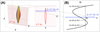Fig. 1. Schematic representation of caustic structure shortly after shell crossing. (A) Left: schematic representation of a 3D Eulerian caustic shortly after shell crossing along the x-axis direction, together with a 2D slice with y = y0 (light red plane). Right: Intersection of the caustic surface with the slice (red curve), also shown in the left panel. (B) Schematic representation of the x component of the Lagrangian coordinate, qx, as a function of the Eulerian coordinate, x, for fixed (y0, z0) (solid blue line). Given x0, the solution of the three-value problem x(qx) = x0 is given by qx, n(x0, y0, z0) for n = 1, 2, and 3, as in Eq. (41).

Axisymmetric dynamics translates as follows on the displacement, Ψ(q):

$$\begin{array}{cc}\hfill {\mathrm{\Psi }}_x(q_x,q_y,q_z)& ={\mathrm{\Psi }}_x(q_x,-q_y,q_z)={\mathrm{\Psi }}_x(q_x,q_y,-q_z)\hfill \\ \hfill & =-{\mathrm{\Psi }}_x(-q_x,q_y,q_z),\hfill \end{array}$$(17)

$$\begin{array}{cc}\hfill {\mathrm{\Psi }}_y(q_x,q_y,q_z)& ={\mathrm{\Psi }}_y(q_x,q_y,-q_z)={\mathrm{\Psi }}_y(-q_x,q_y,q_z)\hfill \\ \hfill & =-{\mathrm{\Psi }}_y(q_x,-q_y,q_z),\hfill \end{array}$$(18)

$$\begin{array}{cc}\hfill {\mathrm{\Psi }}_z(q_x,q_y,q_z)& ={\mathrm{\Psi }}_z(-q_x,q_y,q_z)={\mathrm{\Psi }}_z(q_x,-q_y,q_z)\hfill \\ \hfill & =-{\mathrm{\Psi }}_z(q_x,q_y,-q_z).\hfill \end{array}$$(19)

Here and hereafter, we omit the time dependence in the notations. Expanding these functions around the origin q = 0, we have

$$\begin{array}{cc}\hfill {\mathrm{\Psi }}_x(\mathit{q})& ={\displaystyle \sum _{i,j,k=0}\frac{{\psi }_{2i+12j2k}}{(2i+1)!(2j)!(2k)!}{q}_x^{2i+1}{q}_y^{2j}{q}_z^{2k},}\hfill \end{array}$$(20)

$$\begin{array}{cc}\hfill {\mathrm{\Psi }}_y(\mathit{q})& ={\displaystyle \sum _{i,j,k=0}\frac{{\psi }_{2i2j+12k}}{(2i)!(2j+1)!(2k)!}{q}_x^{2i}{q}_y^{2j+1}{q}_z^{2k},}\hfill \end{array}$$(21)

$$\begin{array}{cc}\hfill {\mathrm{\Psi }}_z(\mathit{q})& ={\displaystyle \sum _{i,j,k=0}}\frac{{\psi }_{2i2j2k+1}}{(2i)!(2j)!(2k+1)!}{q}_x^{2i}{q}_y^{2j}{q}_z^{2k+1},\hfill \end{array}$$(22)

with ψ_i j k being some functions of time. Substituting Eqs. (20)–(22) into Eq. (3), and neglecting O(q⁴) and higher-order terms, we obtain

$$\begin{array}{cc}\hfill x(\mathit{q})& \simeq (1+{\psi }_{100})q_x+\frac{1}{2}({\psi }_{120}{q}_y^2+{\psi }_{102}{q}_z^2)q_x+\frac{1}{6}{\psi }_{300}{q}_x^3,\hfill \end{array}$$(23)

$$\begin{array}{cc}\hfill y(\mathit{q})& \simeq (1+{\psi }_{010})q_y+\frac{1}{2}({\psi }_{012}{q}_z^2+{\psi }_{210}{q}_x^2)q_y+\frac{1}{6}{\psi }_{030}{q}_y^3,\hfill \end{array}$$(24)

$$\begin{array}{cc}\hfill z(\mathit{q})& \simeq (1+{\psi }_{001})q_z+\frac{1}{2}({\psi }_{201}{q}_x^2+{\psi }_{021}{q}_y^2)q_z+\frac{1}{6}{\psi }_{003}{q}_z^3.\hfill \end{array}$$(25)

While this local representation of the motion is minimal, it remains accurate shortly after collapse as illustrated by Appendix A.

We now write the necessary conditions that the coefficients in Eqs. (23)–(25) must satisfy for a pancake to exist near the origin. It is important to note that these conditions do not necessarily imply that a halo subsequently forms, this would require more restrictive constraints.

Since we considered a system in which first shell crossing just took place along the x direction at q = 0, we imposed

$$\begin{array}{cc}\hfill \frac{\partial x(\mathbf{0})}{\partial q_x}& \equiv -h=1+{\psi }_{100}<0,0<h\ll 1,\hfill \end{array}$$(26)

$$\begin{array}{cc}\hfill \frac{\partial y(\mathbf{0})}{\partial q_y}& =1+{\psi }_{010}>0,\hfill \end{array}$$(27)

$$\begin{array}{cc}\hfill \frac{\partial z(\mathbf{0})}{\partial q_z}& =1+{\psi }_{001}>0.\hfill \end{array}$$(28)

Additional constraints can be obtained from the expression of the Jacobian determinant, J = det∂x/∂q at the leading order in q, which reads

$$\begin{array}{c}\hfill J\simeq \frac{1}{2}(1+{\psi }_{010})(1+{\psi }_{001})(-2h+{\psi }_{120}{q}_y^2+{\psi }_{102}{q}_z^2+{\psi }_{300}{q}_x^2).\end{array}$$(29)

From catastrophe theory (see e.g. Hidding et al. 2014; Feldbrugge et al. 2018, and references therein), the caustic surface should be an ellipsoid outside of which the Jacobian determinant must have a positive value J > 0, so we imposed

$$\begin{array}{c}\hfill {\psi }_{120}>0,{\psi }_{102}>0,{\psi }_{300}>0.\end{array}$$(30)

Finally, the smallness of the h parameter induces an additional simplification of Eqs. (23)–(25) if one supposes that Lagrangian coordinates are restricted to lie in the neighbourhood of the pancake, namely q_x ∼ q_y ∼ q_z ∼ 𝒪(h^1/2) from Eq. (29). In this case, one realises that, when examining Eqs. (23)–(25),

$$\begin{array}{cc}\hfill x(\mathit{q})& =\mathcal{O}(h^{3/2}),\hfill \end{array}$$(31)

$$\begin{array}{cc}\hfill y(\mathit{q})& \simeq (1+{\psi }_{010})q_y+\mathcal{O}(h^{3/2}),\hfill \end{array}$$(32)

$$\begin{array}{cc}\hfill z(\mathit{q})& \simeq (1+{\psi }_{001})q_z+\mathcal{O}(h^{3/2}),\hfill \end{array}$$(33)

which implies |x|∼𝒪(h^3/2)≪|y|, |z|∼𝒪(h^1/2), a signature of the pancake nature of the system: the extension of the caustic region along the x-axis is asymptotically infinitely smaller than that along the other axes in the limit h → 0, as illustrated by panel A of Fig. 1. Accordingly, inside and in the vicinity of the caustic region, we can ignore the higher-order terms in the expressions of y and z, and reduce Eqs. (23)–(25) to

$$\begin{array}{cc}\hfill x(\mathit{q})& \simeq (1+{\psi }_{100})q_x+\frac{1}{2}({\psi }_{120}{q}_y^2+{\psi }_{102}{q}_z^2)q_x+\frac{1}{6}{\psi }_{300}{q}_x^3,\hfill \end{array}$$(34)

$$\begin{array}{cc}\hfill y(\mathit{q})& \simeq (1+{\psi }_{010})q_y,\hfill \end{array}$$(35)

$$\begin{array}{cc}\hfill z(\mathit{q})& \simeq (1+{\psi }_{001})q_z.\hfill \end{array}$$(36)

Equations (34)–(36) represent our starting point to derive the x component of the gravitational force inside a pancake.

3.2. The three-value problem

Despite its apparent simplicity, Eq. (14) is not easily exploitable when it comes to estimate the gravitational force analytically, even with as simple expressions as Eqs. (34)–(36). Indeed, although the multi-stream nature of the flow does not appear explicitly in the integral (14), we see in Sect. 3.3 that the calculation of the x component of the gravitational force still requires solving the three-value problem implicit in Eqs. (34)–(36), that is, finding q given x.

From Eqs. (35) and (36), we trivially obtain

$$\begin{array}{c}\hfill q_y=\frac{y}{1+{\psi }_{010}},q_z=\frac{z}{1+{\psi }_{001}}.\end{array}$$(37)

The calculation of q_x(x) is more complex because it requires solving the following cubic equation, as illustrated by panel B of Fig. 1,

$$\begin{array}{c}\hfill q_x^3+3A(y,z)q_x+2B(x)=0,\end{array}$$(38)

where we define

$$\begin{array}{cc}& A(y,z)=\frac{1}{{\psi }_{300}}(-2h+{\psi }_{120}{\left(\frac{y}{1+{\psi }_{010}}\right)}^2+{\psi }_{102}{\left(\frac{z}{1+{\psi }_{001}}\right)}^2),\hfill \end{array}$$(39)

$$\begin{array}{cc}\hfill & B(x)=-\frac{3x}{{\psi }_{300}}.\hfill \end{array}$$(40)

The roots of cubic Eq. (38) are given by (see e.g. Abramowitz & Stegun 1972)

$$\begin{array}{cc}\hfill q_{x,n}(\mathit{x})& ={\omega }^{n-1}\frac{-A(y,z)}{{(\sqrt{D(\mathit{x})}-B(x))}^{1/3}}+{\omega }^{4-n}{(\sqrt{D(\mathit{x})}-B(x))}^{1/3},\hfill \end{array}$$(41)

for n = 1, 2, and 3. Here, the factor ω is one of the complex cubic roots of unity (i.e. $\omega =(-1\pm i\sqrt{3})/2$), which are the solutions of ω² + ω + 1 = 0. We define the discriminant D(x), which determines the properties of the roots (41), by (e.g. Abramowitz & Stegun 1972)

$$\begin{array}{cc}\hfill D(\mathit{x})& ={(A(y,z))}^3+{(B(x))}^2.\hfill \end{array}$$(42)

We first note that the equation D(x) = 0 defines the caustics surfaces in Eulerian space:

$$\begin{array}{c}\hfill [-2h+{\psi }_{120}{\left(\frac{y}{1+{\psi }_{010}}\right)}^2+{\psi }_{102}{\left(\frac{z}{1+{\psi }_{001}}\right)}^2{]}^3+9{\psi }_{300}{x}^2=0.\end{array}$$(43)

According to the sign of D(x), the solutions of the cubic equation, Eq. (38), can then be classified as follows. If D(x) < 0, we are inside the multi-stream region delimited by the caustic surfaces: the cubic equation has three real solutions, with q_x, 2 < q_x, 3 < q_x, 1 and q_x, 2 < 0 < q_x, 1. If D(x) > 0, we are outside the multi-stream region: only q_x, 1 or q_x, 2 is real, and the other solutions are a complex conjugate to each other.

As a final note, from Eq. (43), the maximum values of the Eulerian coordinates of caustics along the x-, y-, and z-axes are given by

$$\begin{array}{cc}\hfill x_{\max }& =\sqrt{\frac{8h^3}{9{\psi }_{300}}},\hfill \end{array}$$(44)

$$\begin{array}{cc}\hfill y_{\max }& =(1+{\psi }_{010})\sqrt{\frac{2h}{{\psi }_{120}}},\hfill \end{array}$$(45)

$$\begin{array}{cc}\hfill z_{\max }& =(1+{\psi }_{001})\sqrt{\frac{2h}{{\psi }_{102}}},\hfill \end{array}$$(46)

Once again, x_max ≪ y_max, z_max in the limit h → 0.

3.3. The force field inside a pancake

We now present the main results of this paper. Focusing on the dynamics just after the first shell crossing along the x direction, we first derive an analytical formula for the x component of the gravitational force after collapse. Next, we discuss orthogonal components and argue that they can be directly approximated by the high-order LPT acceleration.

By zooming in very closely on the multi-stream region, we notice that the structure of the density field becomes almost 1D when h → 0. This follows from the fact the size of the pancake along the x-axis is much smaller than along orthogonal directions (see Eqs. (31)–(33) and also panel A of Fig. 1). Consequently, given the Eulerian position (x, y₀, z₀) for y₀ and z₀ fixed, solving the Poisson Eq. (10), is asymptotically reduced to a 1D problem along the x-axis, as schematically shown in panel B of Fig. 1. In this case, we can neglect local variations of the density along the y and z directions, and Eq. (10) reduces to the following 1D Poisson equation for the x coordinate of the gravitational acceleration,

$$\begin{array}{cc}\hfill \frac{{\mathrm{d}}^2{\varphi }_{\mathrm{p}}(x,y_0,z_0)}{\mathrm{d}{x}^2}& =4\pi G\overline{\rho }{a}^2(1+\delta (x,y_0,z_0)),\hfill \\ \hfill & =4\pi G\overline{\rho }{a}^2\frac{1}{(1+{\psi }_{010})(1+{\psi }_{001})}{\left|\frac{\partial x}{\partial q_x}\right|}^{-1},\hfill \end{array}$$(47)

where, in the second equality, we have used Eq. (5) with Eqs. (34)–(36).

To solve this equation, we followed in the footsteps of Colombi (2015), Taruya & Colombi (2017), and Rampf et al. (2021) and employed a Green function approach to derive the x component of the force in the multi-stream region, F_x(x₀)≃ − dϕ_p(x₀)/dx with x₀ = (x₀,  y₀,  z₀) (inside the pancake, x ∼ h^3/2, and the background contribution $\overline{\varphi }$ is negligible):

$$\begin{array}{cc}\hfill F_x({\mathit{x}}_0)& \simeq {\displaystyle \int }\mathrm{d}x\frac{4\pi G\overline{\rho }{a}^2}{(1+{\psi }_{010})(1+{\psi }_{001})}{\displaystyle \sum _{n=0,1,2}}{\left|\frac{\partial x}{\partial q_{x,n}}\right|}^{-1}\frac{1}{2}[{\mathrm{\Theta }}_{\mathrm{H}}(x-x_0)-{\mathrm{\Theta }}_{\mathrm{H}}(x_0-x)],\hfill \\ \hfill & ={\displaystyle \int }\mathrm{d}{q}_x\frac{4\pi G\overline{\rho }{a}^2}{(1+{\psi }_{010})(1+{\psi }_{001})}\frac{1}{2}[{\mathrm{\Theta }}_{\mathrm{H}}(x(q_x,\frac{y_0}{1+{\psi }_{010}},\frac{z_0}{1+{\psi }_{001}})-x_0)\hfill \\ \hfill & -{\mathrm{\Theta }}_{\mathrm{H}}(x_0-x(q_x,\frac{y_0}{1+{\psi }_{010}},\frac{z_0}{1+{\psi }_{001}}))],\hfill \\ \hfill & =-\frac{4\pi G\overline{\rho }{a}^2}{(1+{\psi }_{010})(1+{\psi }_{001})}[q_{x,1}({\mathit{x}}_0)+q_{x,2}({\mathit{x}}_0)-q_{x,3}({\mathit{x}}_0)]\hfill \\ \hfill & \text{(in the multi-stream region)},\hfill \end{array}$$(48)

where Θ_H represents the Heaviside step function, and the quantities q_x, n are the three-value problem solutions given in Eq. (41). In the first line of Eq. (48), we have dropped the negligible contributions in the 1D Green function that are not proportional to the Heaviside step function.

Interestingly, one can also write, asymptotically,

$$\begin{array}{c}\hfill F_x({\mathit{x}}_0)\simeq {\mathrm{\Gamma }}_x[q_{x,1}({\mathit{x}}_0)]+{\mathrm{\Gamma }}_x[q_{x,2}({\mathit{x}}_0)]-{\mathrm{\Gamma }}_x[q_{x,3}({\mathit{x}}_0)],\end{array}$$(49)

where Γ_x, defined in Eq. (16), is the x coordinate of the LPT acceleration (computed by ignoring shell crossing). This approximation will be tested in Sect. 5.

Equation (48) applies only to the multi-stream region. However, as mentioned above, in the single-stream region, either q_x, 1 or q_x, 2 is real while the two other values are complex conjugate to each other. Taking the real part of right hand side of Eq. (48), the unphysical contribution arising from the complex conjugate solutions vanishes, leaving only the physical contribution from one real solution¹:

$$\begin{array}{cc}\hfill F_x({\mathit{x}}_0)& \simeq -\frac{4\pi G\overline{\rho }{a}^2}{(1+{\psi }_{010})(1+{\psi }_{001})}\mathrm{Re}[q_{x,1}({\mathit{x}}_0)+q_{x,2}({\mathit{x}}_0)-q_{x,3}({\mathit{x}}_0)].\hfill \end{array}$$(51)

Here, ‘Re’ denotes the real part.

Equation (51) is the most important formula in our work. Together with the solution of the cubic Eq. (41), it consists of a simple algebraic form for the x component of the force in the vicinity of the pancake, inside and outside it. This formula is the natural extension to 3D of the 1D calculations of Gurevich & Zybin (1995), Colombi (2015), Taruya & Colombi (2017), and Rampf et al. (2021).

The components F_y and F_z of the force orthogonal to the shell-crossing direction, hence coplanar with the pancake, should, on the other hand, remain quite insensitive to the effects of shell crossing, as we show with numerical tests in following sections. This means that if the LPT displacement field is entirely sourced by gravity, its second time derivative should provide a very good approximation of the local gravitational acceleration, even slightly beyond shell crossing. As a consequence, the acceleration directly derived from the high-order LPT solution (with no Taylor expansion at the third order in q space) should provide a good approximation for F_y and F_z. Of course this is true only if one remains within the convergence radius of the LPT series, which is finite in the general case (e.g. Zheligovsky & Frisch 2014; Rampf et al. 2015; Rampf & Hahn 2021). To overcome the three-value problem, the acceleration can be obtained with the weighted average (15) over the different flows inside the pancake, even though this is not absolutely necessary, since it is expected, in the vicinity of the pancake, that F_y[x(q₁)] ≃ F_y[x(q₂)] ≃ F_y[x(q₃)] and similarly for the z component of the force: this is due to the fact that the vectors q₁, q₂ and q₃ are nearly equal.

4. Examination of the accuracy of the formulas

In this section we test the validity and the accuracy of our prescription for calculating the post-collapse force. To this end, we assume Einstein-de Sitter cosmology and consider simplified initial conditions composed of two or three crossed sine waves, following the early investigations of Moutarde et al. (1991, 1995) and our previous works (Saga et al. 2018). We present these initial conditions in Sect. 4.1, where we also give practical details on the way the analyses are performed. Section 4.2 focuses on the force along the shell-crossing direction. We test, at different orders of the perturbative development, the accuracy of Eq. (51) against the exact solution obtained by direct resolution of Poisson equation. This is followed in Sect. 4.3 by a comparison, in the transverse direction, of the LPT acceleration to the exact force. All these analyses are performed very shortly after collapse to make sure that assumptions of Sect. 3.1 are verified. One indeed expects increasing discrepancies with time between the exact solution and the approximations of the dynamics, as examined in Sect. 4.4.

Throughout this section, we use the LPT solution as a proxy for the ‘exact’ Eulerian position. To calculate the exact force field, we simply injected the LPT solution into Eq. (14) and numerically performed the 2D or 3D integrals². The comparisons to simulations performed in Sect. 5 will show that this proxy turns to provide a quite accurate description of the true displacements at the times we consider.

4.1. Two- and three-sine-wave initial conditions: Practical implementation

We considered initial conditions seeded by two or three crossed sine waves in a periodic box [ − L/2, L/2[ in which the initial displacement field at initial time t_ini is expressed by (see STC)

$$\begin{array}{c}\hfill {\mathrm{\Psi }}_i^{\mathrm{ini}}(\mathit{q},t_{\mathrm{ini}})=\frac{L}{2\pi }{D}_{+}(t_{\mathrm{ini}}){ϵ}_{i}sin\left(\frac{2\pi }{L}{q}_i\right),\end{array}$$(52)

with ϵ_i < 0 and |ϵ_x|≥|ϵ_y|≥|ϵ_z|. The initial density field, ${\delta }^{\mathrm{ini}}\simeq -{\mathbf{\nabla }}_q·{\mathbf{\Psi }}^{\mathrm{ini}}=D_{+}(t_{\mathrm{ini}})\sum _i|{ϵ}_i|cos(2\pi /L{q}_i)$, presents a small peak at the origin. Subsequently, mass elements fall towards the overdense central region, and shell crossing takes place at the origin. The initial time, t_ini, is set to satisfy D₊(t_ini)|ϵ_i|≤0.012 ≪ 1, so that the fastest growing mode approximation is accurate (Saga et al. 2018). We note that in the Einstein-de Sitter universe, the growth factor is simply proportional to the scale factor and we have f = 1. Hence, we hereafter use the scale factor to describe the time rather than D₊.

In this setup, the dynamics is determined by the ratios ϵ_2D = ϵ_y/ϵ_x and ϵ_3D = (ϵ_y/ϵ_x, ϵ_z/ϵ_x), respectively for two- and three-sine-wave initial conditions (STC). We considered three qualitatively different initial conditions, as detailed in Table 1: quasi-1D with |ϵ_x|≫|ϵ_y, z| (Q1D), anisotropic with |ϵ_x|> |ϵ_y|> |ϵ_z| (ANI), and axial-symmetric with |ϵ_x|=|ϵ_y|=|ϵ_z| (SYM). The Q1D and ANI initial conditions are the primary targets of our analyses because first shell crossing occurs only along the x direction, satisfying the assumptions of Sect. 3.1. On the other hand, for the SYM case, since shell crossing takes place simultaneously along two or three axial directions, the prescriptions proposed in Sect. 3.3 to approximate the force field becomes improper. However, the SYM case might provide insight into rare primordial haloes and remains mathematically interesting. In this case, we explore only numerically the force field by comparing predictions of higher-order LPT combined with the Green function approach (Eq. (14)) to measurements in the simulations (see Sect. 5).

Sine wave initial conditions (52) correspond to a low-order trigonometric polynomial, which makes LPT calculations relatively cheap and allows us to reach the 40th and 15th order for the 2D and 3D case, respectively (see Sect. 2 in STC for the explicit procedure)³. Having obtained the higher-order LPT solutions, we analytically predicted the force along the shell-crossing direction using Eq. (51), by expanding the LPT solutions around the origin up to the third order in terms of Lagrangian coordinates to have the expressions for the coefficients ψ_ijk in Eqs. (20)–(22) hence in formula (51). Also, we analytically predicted the force orthogonal to the shell-crossing direction by directly using the LPT acceleration (without Taylor expanding it in q) and averaging it (numerically) over different flows at same Eulerian position x using Eq. (15).

Because the collapse time, traced here by the value of the expansion factor $a_{\mathrm{sc}}^{(n)}$, decreases when perturbative order n augments (see e.g. STC), LPT predictions are in practice synchronised to their own respective shell-crossing times. Then the system is evolved beyond collapse by a very small amount of time:

$$\begin{array}{c}\hfill a^{(n)}=a_{\mathrm{sc}}^{(n)}(1+\mathrm{\Delta }),\end{array}$$(53)

where Δ is a small parameter, such that the assumptions of Sect. 3.1 are valid, in particular h ≃ Δ |∂v_x/∂q_x/(aH)|_{q = 0,  t = tsc} ≪ 1. In practice, we take Δ = 0.001 in Sects. 4.2 and 4.3, while it is allowed to be larger in Sect. 4.4. As a final note, we truncated the integral in Eq. (14) to a finite interval [ − q_max, q_max] in each dimension, setting q_max = L/2 for F_x and q_max = 10L for F_y, z to insure convergence of the integral, as studied in Appendix B.

In the rest of the paper, we use the following units: a box size L = 1 and an inverse of the Hubble parameter at the present time H₀ = 1 for the dimensions of length and time, respectively. We also present the normalised force $\stackrel{\sim }{\mathit{F}}(\mathit{x})$ given by

$$\begin{array}{c}\hfill \stackrel{\sim }{\mathit{F}}(\mathit{x})=\frac{\mathit{F}(\mathit{x})}{4\pi G{a}^2\overline{\rho }}.\end{array}$$(54)

4.2. Force along the shell-crossing direction, F_x

Figure 2 displays, just after shell crossing, the x component of the force F_x as a function of x in the vicinity of the pancake for various values of y. The perturbative order increases from left to right, while initial conditions are given, from top to bottom, by Q1D-2SIN, ANI-2SIN, Q1D-3SIN, and ANI-3SIN.

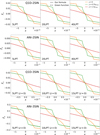Fig. 2. x component of force as a function of x inside and in the vicinity of a pancake seeded by three sine waves in the context of LPT dynamics, with −1.8 ≤ x/xmax ≤ 1.8, where xmax is the maximum extension of the caustic region along the x-axis, as given by Eq. (44) in our approximate formalism. The output time is set to Δ = 0.001 with synchronisation (see Eq. (53)). In each panel, the curves of various colours correspond to different values of y (and z = 0 in the 3D case), namely y/ymax = 0 (orange), 0.75 (green), and 1.5 (red, outside the multi-stream region), where ymax is the maximum extension of the caustic region along the y-axis (Eq. (45)). From top to bottom, we consider Q1D-2SIN, ANI-2SIN, Q1D-3SIN, and ANI-3SIN. From left to right, the predictions are made with 5, 20 (10), and 40LPT (15LPT) for two-sine-wave (three-sine-wave) initial conditions. The dashed and solid lines respectively represent the ‘exact’ force given by Eq. (14) and the analytic prediction (51).

We first notice the perfect agreement between the analytical formula (51) (solid curves) and the exact solution (14) (dashed curves), which fully justifies the mathematical relevance of the formalism developed in Sect. 3. In particular, the sharp transition between the single-stream and the multi-stream region is perfectly described by Eq. (51), with the variations with y (and z, not shown here) accounted for correctly. The discontinuity observed on the derivative of the x component of the force field is a typical signature of the presence of caustics, as found previously in the 1D case (see e.g. Gurevich & Zybin 1995; Colombi 2015), as well as in caustic rings (see e.g. Fig. 8 in Sikivie 1999).

Interestingly, the results do not strongly depend on the perturbation order in Fig. 2. This is because both the analytical formula (51) and the numerical calculation (14) rely on LPT displacement, which shows fast convergence behaviour with LPT order after synchronisation of shell-crossing times (see Fig. 10 in STC).

Obviously, our approach works because parameter Δ in Eq. (53) is very small, which makes the pancake quasi-1D, independently of the values of ϵ_2D and ϵ_3D as long as ϵ_y, ϵ_z < ϵ_x. We see in Sect. 4.4 how the accuracy of the description deteriorates with increasing Δ, that is, with increasing time interval after collapse.

4.3. Force orthogonal to the shell-crossing direction

We now turn to the component F_y of the force orthogonal to the shell-crossing direction (hence coplanar with the pancake) inside and in the vicinity of the pancake, as shown in Fig. 3 very shortly after collapse (note that the plot of the z component, F_z, in the 3D case, would give results very similar to F_y, so is not shown here). As already mentioned in Sect. 3.3, contrary to F_x, the exact gravitational force field given by Eq. (14), displayed as dashed curves, is not significantly affected by the presence of caustics, with a weak dependence on x, F_y ∝ y and F_z ∝ z close to the origin, while F_y and F_z are locally even with respect to z and y, respectively (not shown on the figures). In particular we find, by comparing F_y, z just before and after collapse (Δ = ±0.001), that it hardly changes during this period of time. These results suggest that shell crossing along the x direction does not strongly affect the dynamics along other axes. This property allows us to still use the high-order LPT solution, that is, the acceleration computed as the second time derivative of the LPT displacement, to describe the y and z components of the force as long as the LPT series converges, as shown by the solid curves in Fig. 3 after averaging other the streams according to Eq. (15). The solid curves in Fig. 3 converge to the exact solution when the perturbative order, n, increases, except the 15th order is still insufficient for ANI-3SIN. Convergence is eased when approaching quasi-1D initial conditions (Q1D-2SIN and Q1D-3SIN), thanks to the much faster convergence of the LPT series in this case. We also checked in Eq. (15) that the LPT accelerations computed inside each stream are nearly the same.

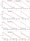Fig. 3. Same as Fig. 2 but for the y component of the force, Fy, in the range −1.8 ≤ y/ymax ≤ 1.8 for x/xmax = 0 (orange), 0.75 (green), and 1.5 (red). The dashed and solid lines represent, respectively, the force given in Eq. (14) and the LPT acceleration given in Eq. (15). Due to the weak dependence of Fy on the presence of the caustic and the very small range of values of x considered, the curves for x/xmax = 0, 0.75, and 1.5 nearly perfectly overlap.

Another important finding is that the dashed curves are only weakly dependent on LPT order, which is a consequence of synchronisation of LPT predictions with their own collapse time. We see in Sect. 5 that they actually agree very well with the measurements in ColDICE simulations. As shown by STC, the density field, which stems from synchronised LPT displacements and sources the force field, is very well described by LPT predictions even of relatively low order. On the other hand, the solid curves in Fig. 3 show that the LPT acceleration converges much more slowly than the LPT displacement, even after synchronisation. This is a rather obvious consequence of the fact that time derivatives give more weight than cumulative quantities to deviations from the exact solution, since these last ones increase with time. Similarly, STC found that convergence of LPT for velocities fields was slower than for density fields. We thus note that Eq. (14) provides, at fixed LPT order, a much more accurate way to compute the gravitational acceleration than the second time derivative of the LPT displacement, as already mentioned in last paragraph of Sect. 2.2. In other words, it provides a re-summation of the gravitational force that could be used to improve on LPT predictions even prior to shell crossing (i.e. even in the absence of synchronisation; see Fig. 6 in Sect. 5).

4.4. Time dependence

In the analyses performed in the two previous sections, we made sure that the assumptions of Sect. 3.1 were valid by taking a very small value of Δ = 0.001 in Eq. (53). In Fig. 4 we investigate how the results change when Δ increases, up to the values ${\mathrm{\Delta }}_{\mathrm{sim}}^{\mathrm{LPT}}={\mathrm{\Delta }}_{\mathrm{sim}}(a_{\mathrm{sc}}/a_{\mathrm{sc}}^{\mathrm{LPT}}),$ with Δ_sim listed in Table 1, that are used for measurements of Sect. 5 in ColDICE simulations.

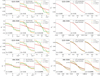Fig. 4. Time dependence of the x and y components of the force for the various initial sine wave conditions considered in this article, as indicated in the panels. In each row, the output time, traced by the parameter Δ in Eq. (53), increases from left to right, as indicated in each panel, with $\mathrm{\Delta }={\mathrm{\Delta }}_{\mathrm{sim}}(a_{\mathrm{sc}}/a_{\mathrm{sc}}^{\mathrm{LPT}})$ in the right panels, where Δsim corresponds to the output time in the simulations discussed in Sect. 5 (see also Table 1). Note that in this last case, the value indicated in the figure is not Δ but Δsim, but the differences are small. The exact solution given by Eq. (14) applied to the LPT displacement (dashes) is compared to the analytical formula (51) for Fx and with the LPT acceleration (15) for Fy (solid lines). The two top and two bottom rows use 40LPT and 15LPT, respectively, to compute the displacement field and its acceleration. In the two bottom rows, we assume z = 0.

We first focus on F_x by examining left panels of Fig. 4. As expected, the analytical prediction (51) deviates more and more from the exact solution as Δ increases. For a given value of Δ, for example Δ = 0.01, deviations are slightly larger for ANI cases than Q1D cases, in agreement with intuition. Yet, even for non Q1D initial conditions, the local quasi-1D nature of the dynamics dominates if Δ is small enough. Obviously our approach has its limits, as illustrated by bottom right panel of the left part of Fig. 4. Importantly, deviations between dashes and solid lines in the left part of Fig. 4 are not related to performances of high-order LPT but instead, to our truncation to the third order of the Taylor expansion in Eqs. (20)–(22), as illustrated by Fig. A.1. This also explains why deviations also increase with the value of y, when passing from the green to the red curve in the left panels of Fig. 4. We note that it would be possible to correct the solutions (41) of the three-value problem by including perturbatively higher-order terms in the Taylor expansion in q, which would most certainly improve the agreement between the solid and the dashed curve in the ANI-3SIN case, even for Δ = 0.0289. Of course, such a procedure cannot apply to arbitrarily large Δ. It would moreover become pointless since LPT becomes a worse prescription of the dynamics as Δ increases. Indeed LPT has a finite convergence radius in time and does not take into account the feedback of the gravitational force inside the caustics, which is the objective we have in mind when computing the force field.

Next, we focused on F_y and examined the right panels of Fig. 4⁴, which confirm what we find in the previous section for Δ = 0.001: except for the ANI-3SIN case, the LPT acceleration given by Eq. (15) agrees well with the exact solution (14) at all times considered. It stays pretty insensitive to the existence of the multi-stream region, as long as the pancake remains very thin and preserves the 1D nature of the local dynamics, which facilitates convergence of the LPT series. This is obviously not the case of ANI-3SIN, where F_y presents significant variations with x that increase with time, especially for the exact solution. We note that the good agreement between theory and exact solution is obviously greatly facilitated by 40LPT in 2D, while only 15LPT is used in the 3D cases. Still, although the Q1D-3SIN case uses only the 15LPT solution for the acceleration, theory and exact solutions still agree very well with each other. On the other hand, in the ANI-3SIN case, the LPT acceleration deviates significantly from the exact force given by Eq. (14) and this even before shell crossing, while the 15LPT displacement itself remains a very good approximation of the true displacement measured in simulations, even for $\mathrm{\Delta }={\mathrm{\Delta }}_{\mathrm{sim}}^{\mathrm{LPT}}$, as shown below in Sect. 5.

5. Comparison to simulations

In the previous sections, we tested the accuracy of force field calculations by using LPT as a proxy of the dynamics. We now rely on actual measurements in Vlasov-Poisson simulations to test LPT itself, since it is used for computing the coefficients in Eqs. (34)–(36) that lead to the asymptotic expression (51) as well as the gravitational acceleration as a second time derivative of the LPT displacement in Eqs. (49) and (15).

The simulations we used to conduct the analyses were performed by Colombi (2021) and STC with the public Vlasov code ColDICE (Sousbie & Colombi 2016). This solver directly follows the evolution of a self-gravitating 3D (2D) phase-space sheet in 6D (4D) phase-space with an adaptive tessellation of tetrahedra (triangles). The initial configuration uses a regular pattern of n_s vertices with null velocities to construct the tessellation. At the beginning of the simulations, this pattern is perturbed with Zel’dovich motion following Eq. (52). During runtime, Poisson equation is solved in ColDICE on a mesh of fixed resolution n_g. Table 1 indicates the values of n_s and n_g adopted for our runs, as well as the expansion factor a_sim of the snapshot used for the analyses slightly beyond first shell crossing. Other technical details on the simulations we used are already provided in Colombi (2021) and STC, so we do not repeat them here. In Appendix C, we explain how we measured the force field from the tessellation.

To compare LPT predictions to measurements in simulations, we proceeded as in Sect. 4 and synchronised high-order LPT solutions (here, 40LPT for the 2D case and 15LPT for the 3D case) as follows. First, LPT solutions were evolved to their own shell-crossing time, designated in Table 1 by $a_{\mathrm{sc}}^{\mathrm{LPT}}$ (namely $a_{\mathrm{sc}}^{(40)}$ and $a_{\mathrm{sc}}^{(15)}$ for 2D and 3D, respectively, in the notations of Sect. 4). Next, time was advanced up to expansion factor $a=a_{\mathrm{sc}}^{\mathrm{LPT}}+(a_{\mathrm{sim}}-a_{\mathrm{sc}})$, where a_sc and a_sim are respectively the shell-crossing time measured by STC in the simulations and the expansion factor of the snapshot we considered for the analyses, as listed in Table 1. We note that the output times of the simulations, which are different for each initial condition, are, in terms of relative expansion factor values, closer to the shell-crossing time in the following order: ANI-2SIN, Q1D-3SIN, Q1D-2SIN, and ANI-3SIN (see the last column in Table 1).

Figure 5 compares analytical predictions to measurements in the simulations of the force field for the various sine wave initial conditions introduced in Sect. 4.1, except the axisymmetric ones, which are discussed further below. The first thing to notice when examining this figure is the excellent agreement between the measurements (black dots) and the numerical solution of Poisson equation based on the Green function approach, Eq. (14), when applied to the density field sourced by the LPT displacement after synchronisation (orange dashes). This confirms the earlier investigations of STC on the density field, which compared post-collapse predictions based on the ballistic approximation, where the velocity field is frozen at collapse time, to the same simulations data. At the times considered here, the ballistic approximation should not differ much from LPT predictions pushed beyond shell crossing as performed in the present work. Such a good agreement between LPT and simulations fully validates the conclusions of the analyses of Sect. 4. Thus, in Fig. 5 we observe the same matches and discrepancies between the solid green (left panels) or blue (right panels) curves and the black dots or orange dashes, respectively, that we can discern in Fig. 4 between the solid curves and the dashes. This confirms again the validity of our theoretical predictions when two conditions are met: (i) sufficiently short period of time after collapse, so that our local Taylor expansion of the displacement field remains accurate enough to estimate the component of the force along the shell-crossing direction (orthogonal to the pancake) with Eq. (51), and (ii) sufficiently high LPT order for the LPT displacement to be accurate around shell-crossing time, as well as its second time derivative used in Eq. (15) as an approximation for the component of the force orthogonal to the direction of collapse (coplanar with the pancake). Obviously, these two conditions are not met for ANI-3SIN as already discussed in detail in Sect. 4, but are facilitated in the Q1D cases.

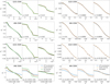Fig. 5. Comparison between simulations and analytical predictions for Fx (left panels) and Fy (right panels) slightly beyond first shell-crossing time. From top to bottom, we consider Q1D-2SIN, ANI-2SIN, Q1D-3SIN, and ANI-3SIN initial conditions, respectively. For each initial condition, we present the force for three different values of y and/or z, as indicated in each panel. The largest values of y and z are outside the multi-stream region. The dots stand for the measurements in the ColDICE simulations. The solid green curves in the left panels give the theoretical prediction for Fx from the analytical formula (51). The solid blue lines correspond to the theoretical predictions for Fx and Fy obtained from the LPT acceleration using Eq. (49) (only in the multi-stream region) and Eq. (15), respectively. The dashed orange lines represent the force field resulting from solving the Poisson Eq. (14), when using the LPT displacement instead of the supposedly exact positions of particles in the ColDICE runs.

Interestingly, Eq. (49) (solid blue curves in the left panels of Fig. 5) approximates very well the x component of the force, except again for ANI-3SIN. Summing up correctly the LPT accelerations in the multi-stream regions using either Eq. (49) or Eq. (15) also provides, shortly after shell crossing, a very good self-consistent approximation of all the components of the force field provided that the LPT series is converged.

The synchronisation process plays an important role in the analytical prediction of the force along the direction of shell crossing, F_x, because collapse time changes with LPT order and the effect of shell crossing is dramatic on F_x. However, this is not really the case for the orthogonal component – coplanar with the pancake – that pretty much preserves the single-stream behaviour of the motion, as already discussed in Sect. 4.3. We double-checked this property by reproducing the right panels of Fig. 5 on Fig. 6 but without synchronisation of LPT predictions. For the 40th LPT order and the 15th LPT order respectively in 2D and 3D, we indeed distinguish no difference between the two figures. Additionally, various LPT orders are considered on Fig. 6. Interestingly, the LPT accelerations (solid lines) show slow convergence, while the forces computed with the Green function method from the LPT displacements (Eq. (14), dashed lines) show very fast convergence, even for ANI-3SIN. In other words, as mentioned in Sect. 4.3, Eq. (14) represents a re-summation of LPT that provides a much more accurate description of the gravitational acceleration than the second time derivative of the LPT displacement. This property might turn very useful for future applications.

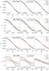Fig. 6. Same as the right panels of Fig. 5, but without synchronisation to collapse time at each LPT order, i.e. for a given initial condition, all the curves are calculated at the same expansion factor, asim. In addition, several LPT orders are considered, as indicated in the right panels, to illustrate the convergence speed.

Before closing this section, we examine in Fig. 7 axial-symmetric initial conditions, SYM-2SIN and SYM-3SIN. In this case, shell crossing occurs simultaneously along all the axes of the dynamics, so we expect qualitatively different behaviour from the Q1D and ANI cases. Strictly speaking, axial-symmetric configurations have zero weight from the statistical point of view but can in practice still be present at the coarse level, for example a very high peak in random Gaussian fields that are expected to be rounder (see e.g. Bardeen et al. 1986).

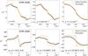Fig. 7. Same as Fig. 5 but for the SYM-2SIN (top panels) and SYM-3SIN (bottom panels) initial conditions and the fact that there are no blue or green curves, because our analytical recipes apply only to shell crossing occurring along one direction. Only the x component of the force is shown in Fig. 7 due to the symmetric nature of the system. In addition, the 15LPT prediction from Eq. (14) is shown as a dashed light orange curve in the 2D case.

The axisymmetric case does not correspond to the superposition of 2 and 3 pancakes in the 2D and 3D cases, respectively (see Gurevich & Zybin 1995, for analytical predictions of the gravitational potential under these assumptions). Indeed, the caustic structure stemming from simultaneous shell crossings along several directions is convoluted, as shown by STC, which translates into multiple discontinuities of the derivative of the force field along each axis. For instance, in the top-left panel of Fig. 7 there are four sharp transition points on the force field instead of the two in the top-left panel of Fig. 5. Even if the analytical predictions discussed in Sect. 3 are irrelevant for SYM cases, it is still possible to use the Green function approach in Eq. (14) with the high-order LPT displacement field used as a proxy for the dynamics, as indicated by the dashed curves on Fig. 7. While 40LPT successfully reproduces the post-collapse gravitational field in the 2D case, 15LPT is not accurate enough. Turning to the 3D case, 15LPT is not even good from the qualitative point of view, as already noticed for STC for the density field itself. However, SYM-3SIN is further away from shell crossing than SYM-2SIN in terms of the parameter Δ as shown in last column of Table 1, which explains partly the worse performance of LPT predictions for SYM-3SIN compared to SYM-2SIN. Another and more obvious reason for this lies in the much higher contrasts expected in SYM-3SIN compared to SYM-2SIN, which can introduce non negligible feedback effects from the multi-stream region, even very shortly after shell crossing, as already extensively discussed in STC.

6. Summary

In this article we have studied the gravitational force field generated by pancakes shortly after collapse. Restricting ourselves to the case where the displacement field sourcing the pancake is locally symmetric, we derived approximations for the force field by combining fundamentals of catastrophe theory and high-order LPT that we carefully validated on systems seeded by two- or three-sine-wave initial conditions. Our analyses include comparisons of theoretical predictions to measurements in Vlasov simulations performed with the public code ColDICE. The important assumption we made is that the time lapse after collapse, quantified here by the parameter Δ given in Eq. (53), is very short, allowing one to assume that the multi-stream region is locally infinitely thin. The main results of our work can be summarised as follows:

• (i)

  The calculation of the component F_x, the gravitational force aligned with the direction of the shell crossing (that is, orthogonal to the pancake), comes down to solving a three-value problem that reduces to the resolution of a third-order polynomial in the limit Δ ≪ 1. This process is very analogous, not surprisingly, to the 1D case and leads to explicit expressions in terms of Eulerian coordinates, Eqs. (37), (39)–(41), and (51). Calculation of the various time-dependent coefficients intervening in the expression of F_x relies on a Taylor expansion of the LPT displacement at the third order in the Lagrangian position, while staying within the convergence radius of the displacement expanded as a high-order series in time.

• (ii)

  The component F_y (and F_z), the gravitational force orthogonal to the direction of shell crossing (that is, in the same plane as the pancake), is rather insensitive to the presence of caustics. It can thus be predicted with the usual LPT acceleration, that is, the second time derivative of the LPT displacement, as long as the LPT acceleration converges as a series expansion in time. While Eq. (15) can be used to perform averaging over several streams, it is not absolutely needed. However, the three-value problem still needs to be solved, either numerically as we did in this work or approximately using Eqs. (37), (39)–(41).

• (iii)

  Equation (51) is asymptotically equivalent to Eq. (49), with the x component of the acceleration given by the second time derivative of the LPT displacement, which in turn makes the approach fully consistent with point (ii).

• (iv)

  A much higher LPT order is needed for the acceleration to converge than for the displacement. This is a natural consequence of the properties of the LPT series, of which the convergence speed decreases with successive time derivatives (see e.g. Rampf et al. 2023). However, one can numerically solve the Poisson equation using the Green function approach embodied by integral Eq. (14) based on the knowledge of the LPT displacement to reach – as is obvious – a convergence level that is as good as for the displacement. Hence, Eq. (14) acts as a re-summation procedure of LPT for accurately computing the gravitational field.

• (v)

  While quasi-1D initial conditions facilitate convergence of PT predictions, our calculations also apply to pancakes seeded by peaks with a general ellipsoid shape and remain accurate as long as the pancake remains very flat, but become inaccurate in the extreme case where collapse takes place simultaneously along all the axes of the dynamics.

In this work we have used LPT as an approximation of the dynamics shortly beyond collapse, but there are limitations to such an approach due to the finite radius of convergence with respect to time of the perturbative series. A safer point of view, adopted and tested successfully by STC on our sine wave cases, consists in using a ballistic approximation, where velocities (and in the present case, LPT accelerations) are frozen from collapse. While for the sake simplicity we did not adopt it here, it would be easy to implement this ballistic approximation to compute the gravitational force field of pancakes instead of using the procedure described in points (i) and (ii). The advantage of the ballistic approach is it allows us to overcome the problem of LPT convergence, which is known to be guaranteed in practice up to collapse (see e.g. Rampf & Hahn 2021, STC).

The calculations presented in this work can in principle be generalised to an arbitrary (smooth and non-degenerate) displacement field. Clearly, the case of a displacement field deriving from a potential in Lagrangian space (i.e. vorticity-free in Lagrangian space) can be treated easily. While not fully representative of the exact dynamics, since zero vorticity prior to shell crossing is only expected in Eulerian space, a vorticity-free displacement in Lagrangian space remains a very good approximation up to the second order in the LPT framework, which includes the Zel’dovich approximation. In the case of a displacement field deriving from a potential, it is easy to see that, with the proper combination of affine transformations in both Lagrangian and Eulerian space, one can obtain equations similar to Eqs. (34)–(36), but with additional $q_x^2{q}_y$, $q_x^2{q}_z$, $q_y^3$, and $q_z^3$ terms in the right-hand side of Eq. (34), which makes solving the three-value problem and the force field calculation slightly more involved. We postpone more general analyses that do not impose the local symmetries (18)–(19) to future work.

The calculation of the force field generated in the vicinity of a proto-pancake represents the first step towards an accurate treatment of the dynamics in the multi-stream regime. It involves computing corrections to the motion inside the pancakes due to the force backreaction from the multi-stream regions, thereby extending the 1D calculations of Colombi (2015), Taruya & Colombi (2017), and Rampf et al. (2021) to the 3D case. Of course, this approach remains limited, as it is expected to work only shortly after shell crossing, though it might be possible to combine it with an adaptive smoothing procedure to accurately predict large-scale structure statistics, such as the power spectrum, even in the non-linear regime (see e.g. Taruya & Colombi 2017; Halle et al. 2020, for the 1D case). Shell crossing can also locally take place along other axes of the dynamics, leading to the formation of proto-filaments and proto-haloes. This is also followed by violent relaxation, which is a quick folding of the phase-space sheet in multiple directions. Understanding in detail the early evolution of proto-pancakes remains crucial to understanding how multi-flow dynamics is initiated and how this affects the early evolution of the statistics of the large-scale matter distribution.

Acknowledgments

We thank C. Rampf for reading and commenting on the draft. S.S. is supported by JSPS Overseas Research Fellowships. This work was supported in part by MEXT/JSPS KAKENHI Grant Numbers JP20H05861 and JP21H01081 (AT), ANR grant ANR-13-MONU-0003 (SC), as well as Programme National Cosmology et Galaxies (PNCG) of CNRS/INSU with INP and IN2P3, co-funded by CEA and CNES (SC). Numerical computation with ColDICE was carried out using the HPC resources of CINES (Occigen supercomputer) under the GENCI allocations c2016047568, 2017-A0040407568 and 2018-A0040407568. Post-treatment of ColDICE data were performed on HORIZON cluster of Institut d’Astrophysique de Paris.

References

Appendix A: Series expansion of the displacement field

In Sect. 3.1 we derive an analytical expression for computing the x component of gravitational force, starting from the Taylor expansion of the displacement field with respect to the Lagrangian coordinate up to the third order in q, given in Eqs. (23)–(25). Figure A.1 tests the accuracy of Eqs. (23)–(25) in q_x-x space for our non-axisymmetric three-sine-wave setups. Clearly, at the dynamical times considered in this paper, a third-order approximation for the displacement field is sufficient in the Q1D case, but significant deviations can be seen in the bottom-right panel of the figure. As expected, these deviations increase when moving away from the origin of coordinates, hence with increasing, |x|, |y| (and |z| in 3D). They explain, at least partly, the discrepancies between theory and exact solution in Fig. 4. Another significant source of error is the approximation of y and z coordinates at the linear order in q (Eqs. 35 and 36), which we do not examine here. W note that, as long as higher-order corrections remain small, it would be possible to correct perturbatively the three-value solution derived from the third-order Taylor expansion to include higher-order contributions. Here, we notice that the fifth order already brings very significant improvements, though we should also check what happens in other planes.

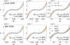Fig. A.1. x coordinate as a function of qx for Q1D-3SIN (top panels) and ANI-3SIN (bottom panels) initial conditions at various output times, with Δ = 0.005 (left), 0.01 (centre), and Δsim = asim/asc − 1, as given in the right column of Table 1 (right). The solid and dashed curves correspond to qy = 0 and $q_y\simeq q_y^{\text{max}}$, where $q_y^{\text{max}}$ is the maximum extension of the caustic in Lagrangian space along the qy-axis, while qz = 0. We present the results predicted by the pure 15LPT solution (black) and its Taylor expansion expression in the Lagrangian coordinate up to up to 𝒪(q3) (orange) and up to 𝒪(q5) (blue).

Appendix B: Calculation of the force: Truncation of integral (14)

Throughout this article, we compare our analytical predictions for the force to direct calculations of the integral (14) over a finite interval, [ − q_max, q_max]. Our systems seeded by initial sine wave conditions are periodic, and hence the problem comes down to computing the gravitational contribution of each matter element inside the simulation volume of size L, plus all the periodic replica. Many techniques exist in the literature to perform such a calculation quickly, for instance Ewald summation (see e.g. Hernquist et al. 1991). Our brute force technique allows us to have rather accurate estimates of pairwise interactions between nearby elements of mass, which is necessary given the very thin nature of the caustic structures, but fails to account for the contribution of all remote elements, including replica, which can make the force field calculation inaccurate.

To validate the choice of our somewhat simplistic technique, Fig. B.1 presents the x (top panels) and y components (bottom panels) of the force for our (non-axisymmetric) sine wave initial conditions, restricting to the local neighbourhood of the pancake. All the output times are the same as in Fig. 5, which compares analytical predictions to simulations. We see that the x component of the force at the scales of interest is dominated by the influence of the caustics and is thus quite insensitive to the replica given these small values of x, so a truncation of the integral (14) at q_max = L/2 is enough for all the initial conditions (including SYM-2SIN and SYM-3SIN, not shown in Fig. 5). On the other hand, the y component of the force can be significantly affected by the replicas for Q1D initial conditions, but from lower panels of Fig. 5, q_max = 5L/2 seems sufficient for adequate convergence of the integral (14). In practice, we adopted the values listed in Table C.1 for the measurements in the ColDICE simulations, and q_max = L/2 for F_x, q_max = 20L/2 for F_y, z, for other calculations using the LPT displacement in Eq. (14).

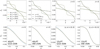Fig. B.1. Tests of the choice of the bounds of integral (14). The x and y coordinates of the force are plotted, respectively, in the top and bottom panels, for various choices of the integration range [ − qmax, qmax] with qmax ranging from L/2 to 20L/2, as indicated in the upper-left panel. From left to right, we consider Q1D-2SIN, ANI-2SIN, Q1D-3SIN, and ANI-3SIN initial conditions. In the top panels, various values of y are considered, as indicated in the second panel of the top row, while the bottom panels only assume x = 0 since other values of x would not lead to significantly different results. We also set z = 0 in the 3D cases considered in the two top-right and two bottom-right panels. Note that the output time chosen in this figure is the same as in Fig. 5. We see that all the curves corresponding to different values of qmax are superimposed on each other, except for qmax = L/2 for the Q1D cases.

Appendix C: Force measurement in simulations

In ColDICE, the dark matter distribution is represented with an adaptive tessellation of simplices, that is, an ensemble of connected triangles and tetrahedra, respectively in 2D and 3D. To compute the force field $\stackrel{\sim }{\mathit{F}}(\mathit{x})$ at a given point of space, we employed a direct approach consisting in replacing each simplex with a set of particles. To do so, if needed, each simplex was refined isotropically ℓ_max times. At the end, each sub-simplex was replaced with a single particle lying at the barycentre of the its vertices. To obtain the highest accuracy, the refinement process exploits the quadratic nature of each simplex thanks to additional tracers used in ColDICE. To avoid divergences due to the singular nature of the force field induced by a point particle distribution, we introduced additional softening as follows:

$$\begin{array}{c}\hfill \stackrel{\sim }{\mathit{F}}(\mathit{x})=\frac{m}{2^{d-2}\times 2\pi }\frac{\mathit{x}-{\mathit{x}}_0}{(|\mathit{x}-{\mathit{x}}_0{{|}^2+{\epsilon }^2)}^{d/2}},\end{array}$$(C.1)

where, d = 2 or 3 is the dimension of space, m and x₀ are respectively the (normalised) mass and the position of the particle. This equation does not account for the background correction proportional to x in Eq. (14), which has to be added at the end of the calculation. Depending on the coordinate of the force field considered, a set of periodic replica of each particle with positions

$$\begin{array}{c}\hfill {\mathit{x}}_0+(i,j,k)L\end{array}$$(C.2)

can contribute, with integers i, j, k ∈ [ − n_rep, n_rep], which is equivalent to restricting the integral (14) to the interval [ − q_max, q_max], with q_max = (n_rep + 1/2)L. The values of q_max we adopted are listed in Table C.1. They are large enough according to the convergence tests discussed in Appendix B.

Because we examined the system just after shell crossing, it is important to have an accurate description of the phase-space sheet inside a region containing the caustics. This region was chosen to be a thin rectangular parallelepiped covering the intervals x ∈ [ − x_max, x_max], y ∈ [ − y_max, y_max], and z ∈ [ − z_max, z_max] in each dimension (except for the last one, which is in 3D only). Outside this region, each simplex was replaced with a single particle and inside it, each simplex was adaptively refined ℓ_max ≥ 1 times, with a value of ℓ_max depending on initial conditions.

The various parameters introduced in this appendix are listed in Table C.1, which completes Table 1 of the main text. W note, for instance, that ε = x_max/64. Because of the high mass resolution of the 2D simulations (n_s = 2048), is was enough to take ℓ_max = 2 for Q1D-2SIN, ANI-2SIN and SYM-2SIN. Furthermore, due to the lower cost of the force calculation in 2D, many periodic replica could be used, n_rep = 30. On the other hand, the 3D case is much more involved computationally, which imposes us to adopt a much smaller value of n_rep, yet still large enough according to the tests performed in Appendix B. The most delicate case was Q1D-3SIN, where ℓ_max = 4 was necessary to have (barely) sufficiently accurate measurements of the force field. There are two reasons for this. First, in this simulation, the initial tessellation has a lower number of simplices, $6\times n_{\text{s}}^3$, with n_s = 256, compared to n_s = 512 for ANI-3SIN and SYM-3SIN, which already imposes at least one additional refinement level in Q1D-3SIN compared to the two other cases. Second, the discrete nature of the sampling of the phase-space sheet we adopted can introduce systematic biases to the force field that are stronger in Q1D settings due to the fact that particles, which initially form a regular mesh, tend to cluster together much more along the x direction inside and in the vicinity of the caustics than in orthogonal direction(s). This induces artificial fluctuations to the force field, especially on axes orthogonal to x (see e.g. middle panel of the right group in third row of Fig. 5), that would not appear with a proper, smooth representation of the phase-space sheet. While it would be possible (but not trivial) to implement a more optimal calculation of the force field, we did not find it necessary for our analyses.

All Tables

All Figures

Fig. 1. Schematic representation of caustic structure shortly after shell crossing. (A) Left: schematic representation of a 3D Eulerian caustic shortly after shell crossing along the x-axis direction, together with a 2D slice with y = y0 (light red plane). Right: Intersection of the caustic surface with the slice (red curve), also shown in the left panel. (B) Schematic representation of the x component of the Lagrangian coordinate, qx, as a function of the Eulerian coordinate, x, for fixed (y0, z0) (solid blue line). Given x0, the solution of the three-value problem x(qx) = x0 is given by qx, n(x0, y0, z0) for n = 1, 2, and 3, as in Eq. (41).

In the text

Fig. 2. x component of force as a function of x inside and in the vicinity of a pancake seeded by three sine waves in the context of LPT dynamics, with −1.8 ≤ x/xmax ≤ 1.8, where xmax is the maximum extension of the caustic region along the x-axis, as given by Eq. (44) in our approximate formalism. The output time is set to Δ = 0.001 with synchronisation (see Eq. (53)). In each panel, the curves of various colours correspond to different values of y (and z = 0 in the 3D case), namely y/ymax = 0 (orange), 0.75 (green), and 1.5 (red, outside the multi-stream region), where ymax is the maximum extension of the caustic region along the y-axis (Eq. (45)). From top to bottom, we consider Q1D-2SIN, ANI-2SIN, Q1D-3SIN, and ANI-3SIN. From left to right, the predictions are made with 5, 20 (10), and 40LPT (15LPT) for two-sine-wave (three-sine-wave) initial conditions. The dashed and solid lines respectively represent the ‘exact’ force given by Eq. (14) and the analytic prediction (51).

In the text

Fig. 3. Same as Fig. 2 but for the y component of the force, Fy, in the range −1.8 ≤ y/ymax ≤ 1.8 for x/xmax = 0 (orange), 0.75 (green), and 1.5 (red). The dashed and solid lines represent, respectively, the force given in Eq. (14) and the LPT acceleration given in Eq. (15). Due to the weak dependence of Fy on the presence of the caustic and the very small range of values of x considered, the curves for x/xmax = 0, 0.75, and 1.5 nearly perfectly overlap.

In the text

Fig. 4. Time dependence of the x and y components of the force for the various initial sine wave conditions considered in this article, as indicated in the panels. In each row, the output time, traced by the parameter Δ in Eq. (53), increases from left to right, as indicated in each panel, with $\mathrm{\Delta }={\mathrm{\Delta }}_{\mathrm{sim}}(a_{\mathrm{sc}}/a_{\mathrm{sc}}^{\mathrm{LPT}})$ in the right panels, where Δsim corresponds to the output time in the simulations discussed in Sect. 5 (see also Table 1). Note that in this last case, the value indicated in the figure is not Δ but Δsim, but the differences are small. The exact solution given by Eq. (14) applied to the LPT displacement (dashes) is compared to the analytical formula (51) for Fx and with the LPT acceleration (15) for Fy (solid lines). The two top and two bottom rows use 40LPT and 15LPT, respectively, to compute the displacement field and its acceleration. In the two bottom rows, we assume z = 0.

In the text

Fig. 5. Comparison between simulations and analytical predictions for Fx (left panels) and Fy (right panels) slightly beyond first shell-crossing time. From top to bottom, we consider Q1D-2SIN, ANI-2SIN, Q1D-3SIN, and ANI-3SIN initial conditions, respectively. For each initial condition, we present the force for three different values of y and/or z, as indicated in each panel. The largest values of y and z are outside the multi-stream region. The dots stand for the measurements in the ColDICE simulations. The solid green curves in the left panels give the theoretical prediction for Fx from the analytical formula (51). The solid blue lines correspond to the theoretical predictions for Fx and Fy obtained from the LPT acceleration using Eq. (49) (only in the multi-stream region) and Eq. (15), respectively. The dashed orange lines represent the force field resulting from solving the Poisson Eq. (14), when using the LPT displacement instead of the supposedly exact positions of particles in the ColDICE runs.

In the text

	Fig. 6. Same as the right panels of Fig. 5, but without synchronisation to collapse time at each LPT order, i.e. for a given initial condition, all the curves are calculated at the same expansion factor, asim. In addition, several LPT orders are considered, as indicated in the right panels, to illustrate the convergence speed.
In the text

Fig. 7. Same as Fig. 5 but for the SYM-2SIN (top panels) and SYM-3SIN (bottom panels) initial conditions and the fact that there are no blue or green curves, because our analytical recipes apply only to shell crossing occurring along one direction. Only the x component of the force is shown in Fig. 7 due to the symmetric nature of the system. In addition, the 15LPT prediction from Eq. (14) is shown as a dashed light orange curve in the 2D case.

In the text

Fig. A.1. x coordinate as a function of qx for Q1D-3SIN (top panels) and ANI-3SIN (bottom panels) initial conditions at various output times, with Δ = 0.005 (left), 0.01 (centre), and Δsim = asim/asc − 1, as given in the right column of Table 1 (right). The solid and dashed curves correspond to qy = 0 and $q_y\simeq q_y^{\text{max}}$, where $q_y^{\text{max}}$ is the maximum extension of the caustic in Lagrangian space along the qy-axis, while qz = 0. We present the results predicted by the pure 15LPT solution (black) and its Taylor expansion expression in the Lagrangian coordinate up to up to 𝒪(q3) (orange) and up to 𝒪(q5) (blue).

In the text

Fig. B.1. Tests of the choice of the bounds of integral (14). The x and y coordinates of the force are plotted, respectively, in the top and bottom panels, for various choices of the integration range [ − qmax, qmax] with qmax ranging from L/2 to 20L/2, as indicated in the upper-left panel. From left to right, we consider Q1D-2SIN, ANI-2SIN, Q1D-3SIN, and ANI-3SIN initial conditions. In the top panels, various values of y are considered, as indicated in the second panel of the top row, while the bottom panels only assume x = 0 since other values of x would not lead to significantly different results. We also set z = 0 in the 3D cases considered in the two top-right and two bottom-right panels. Note that the output time chosen in this figure is the same as in Fig. 5. We see that all the curves corresponding to different values of qmax are superimposed on each other, except for qmax = L/2 for the Q1D cases.

In the text

References

- Abramowitz, M., & Stegun, I. A. 1972, Handbook of Mathematical Functions, National Bureau of Standards Applied Mathematics Series, 55 [Google Scholar]
- Alard, C. 2013, MNRAS, 428, 340 [Google Scholar]
- Angulo, R. E., Hahn, O., Ludlow, A. D., & Bonoli, S. 2017, MNRAS, 471, 4687 [Google Scholar]
- Arnold, V. I., Shandarin, S. F., & Zeldovich, I. B. 1982, Geophys. Astrophys. Fluid Dyn., 20, 111 [NASA ADS] [CrossRef] [Google Scholar]
- Baldauf, T., Mercolli, L., & Zaldarriaga, M. 2015, Phys. Rev. D, 92, 123007 [NASA ADS] [CrossRef] [Google Scholar]
- Bardeen, J. M., Bond, J. R., Kaiser, N., & Szalay, A. S. 1986, ApJ, 304, 15 [Google Scholar]
- Baumann, D., Nicolis, A., Senatore, L., & Zaldarriaga, M. 2012, J. Cosmol. Astropart. Phys., 2012, 051 [CrossRef] [Google Scholar]
- Bernardeau, F. 1994, ApJ, 427, 51 [NASA ADS] [CrossRef] [Google Scholar]
- Bernardeau, F., Colombi, S., Gaztañaga, E., & Scoccimarro, R. 2002, Phys. Rep., 367, 1 [Google Scholar]
- Bernardeau, F., Crocce, M., & Scoccimarro, R. 2008, Phys. Rev. D, 78, 103521 [NASA ADS] [CrossRef] [Google Scholar]
- Bernardeau, F., Crocce, M., & Scoccimarro, R. 2012, Phys. Rev. D, 85, 123519 [NASA ADS] [CrossRef] [Google Scholar]
- Bernardeau, F., Taruya, A., & Nishimichi, T. 2014, Phys. Rev. D, 89, 023502 [NASA ADS] [CrossRef] [Google Scholar]
- Bertschinger, E. 1985, ApJS, 58, 39 [Google Scholar]
- Beutler, F., Seo, H.-J., Saito, S., et al. 2017, MNRAS, 466, 2242 [Google Scholar]
- Blake, C., Brough, S., Colless, M., et al. 2011, MNRAS, 415, 2876 [NASA ADS] [CrossRef] [Google Scholar]
- Blas, D., Garny, M., & Konstandin, T. 2014, J. Cosmol. Astropart. Phys., 2014, 010 [CrossRef] [Google Scholar]
- Blumenthal, G. R., Faber, S. M., Primack, J. R., & Rees, M. J. 1984, Nature, 311, 517 [Google Scholar]
- Bouchet, F. R., Juszkiewicz, R., Colombi, S., & Pellat, R. 1992, ApJ, 394, L5 [Google Scholar]
- Bouchet, F. R., Colombi, S., Hivon, E., & Juszkiewicz, R. 1995, A&A, 296, 575 [NASA ADS] [Google Scholar]
- Buchert, T. 1992, MNRAS, 254, 729 [NASA ADS] [CrossRef] [Google Scholar]
- Buchert, T., & Ehlers, J. 1993, MNRAS, 264, 375 [Google Scholar]
- Carrasco, J. J. M., Hertzberg, M. P., & Senatore, L. 2012, J. High Energy Phys., 2012, 82 [CrossRef] [Google Scholar]
- Carron, J., & Szapudi, I. 2013, MNRAS, 432, 3161 [Google Scholar]
- Chakrabarty, S. S., & Sikivie, P. 2018, Phys. Rev. D, 98, 103009 [NASA ADS] [CrossRef] [Google Scholar]
- Charmousis, C., Onemli, V., Qiu, Z., & Sikivie, P. 2003, Phys. Rev. D, 67, 103502 [NASA ADS] [CrossRef] [Google Scholar]
- Colombi, S. 2015, MNRAS, 446, 2902 [Google Scholar]
- Colombi, S. 2021, A&A, 647, A66 [NASA ADS] [CrossRef] [EDP Sciences] [Google Scholar]
- Crocce, M., & Scoccimarro, R. 2006, Phys. Rev. D, 73, 063520 [NASA ADS] [CrossRef] [Google Scholar]
- Crocce, M., & Scoccimarro, R. 2008, Phys. Rev. D, 77, 023533 [NASA ADS] [CrossRef] [Google Scholar]
- d’Amico, G., Gleyzes, J., Kokron, N., et al. 2020, J. Cosmol. Astropart. Phys., 2020, 005 [CrossRef] [Google Scholar]
- Delos, M. S., Erickcek, A. L., Bailey, A. P., & Alvarez, M. A. 2018a, Phys. Rev. D, 97, 041303 [Google Scholar]
- Delos, M. S., Erickcek, A. L., Bailey, A. P., & Alvarez, M. A. 2018b, Phys. Rev. D, 98, 063527 [Google Scholar]
- Delos, M. S., & White, S. D. M. 2022, ArXiv e-prints [arXiv:2209.11237] [Google Scholar]
- Delos, M. S., & White, S. D. M. 2023, MNRAS, 518, 3509 [Google Scholar]
- Diemand, J., Moore, B., & Stadel, J. 2005, Nature, 433, 389 [Google Scholar]
- Duffy, L. D., & Sikivie, P. 2008, Phys. Rev. D, 78, 063508 [NASA ADS] [CrossRef] [Google Scholar]
- Feldbrugge, J., van de Weygaert, R., Hidding, J., & Feldbrugge, J. 2018, J. Cosmol. Astropart. Phys., 2018, 027 [CrossRef] [Google Scholar]
- Fillmore, J. A., & Goldreich, P. 1984, ApJ, 281, 1 [Google Scholar]
- Garny, M., Laxhuber, D., & Scoccimarro, R. 2023a, Phys. Rev. D, 107, 063539 [NASA ADS] [CrossRef] [Google Scholar]
- Garny, M., Laxhuber, D., & Scoccimarro, R. 2023b, Phys. Rev. D, 107, 063540 [NASA ADS] [CrossRef] [Google Scholar]
- Gouda, N., & Nakamura, T. 1988, Prog. Theor. Phys., 79, 765 [CrossRef] [Google Scholar]
- Gurevich, A. V., & Zybin, K. P. 1995, Phys.-Usp., 38, 687 [NASA ADS] [CrossRef] [Google Scholar]
- Gurzadyan, V. G., Fimin, N. N., & Chechetkin, V. M. 2023, A&A, 672, A95 [NASA ADS] [CrossRef] [EDP Sciences] [Google Scholar]
- Halle, A., Nishimichi, T., Taruya, A., Colombi, S., & Bernardeau, F. 2020, MNRAS, 499, 1769 [NASA ADS] [CrossRef] [Google Scholar]
- Henriksen, R. N., & Widrow, L. M. 1995, MNRAS, 276, 679 [Google Scholar]
- Hernquist, L., Bouchet, F. R., & Suto, Y. 1991, ApJS, 75, 231 [NASA ADS] [CrossRef] [Google Scholar]
- Hertzberg, M. P. 2014, Phys. Rev. D, 89, 043521 [NASA ADS] [CrossRef] [Google Scholar]
- Hidding, J., Shandarin, S. F., & van de Weygaert, R. 2014, MNRAS, 437, 3442 [Google Scholar]
- Hjorth, J., & Williams, L. L. R. 2010, ApJ, 722, 851 [Google Scholar]
- Ishiyama, T. 2014, ApJ, 788, 27 [Google Scholar]
- Ivanov, M. M., Simonović, M., & Zaldarriaga, M. 2020, J. Cosmol. Astropart. Phys., 2020, 042 [CrossRef] [Google Scholar]
- Lynden-Bell, D. 1967, MNRAS, 136, 101 [Google Scholar]
- Matsubara, T. 2008, Phys. Rev. D, 77, 063530 [NASA ADS] [CrossRef] [Google Scholar]
- Matsubara, T. 2011, Phys. Rev. D, 83, 083518 [NASA ADS] [CrossRef] [Google Scholar]
- Matsubara, T. 2015, Phys. Rev. D, 92, 023534 [Google Scholar]
- Melott, A. L., & Shandarin, S. F. 1989, ApJ, 343, 26 [NASA ADS] [CrossRef] [Google Scholar]
- Moutarde, F., Alimi, J. M., Bouchet, F. R., Pellat, R., & Ramani, A. 1991, ApJ, 382, 377 [Google Scholar]
- Moutarde, F., Alimi, J. M., Bouchet, F. R., & Pellat, R. 1995, ApJ, 441, 10 [NASA ADS] [CrossRef] [Google Scholar]
- Natarajan, A., & Sikivie, P. 2006, Phys. Rev. D, 73, 023510 [NASA ADS] [CrossRef] [Google Scholar]
- Natarajan, A., & Sikivie, P. 2007, Phys. Rev. D, 76, 023505 [NASA ADS] [CrossRef] [Google Scholar]
- Navarro, J. F., Frenk, C. S., & White, S. D. M. 1996, ApJ, 462, 563 [Google Scholar]
- Navarro, J. F., Frenk, C. S., & White, S. D. M. 1997, ApJ, 490, 493 [Google Scholar]
- Nishimichi, T., Bernardeau, F., & Taruya, A. 2016, Phys. Lett. B, 762, 247 [Google Scholar]
- Novikov, E. A. 1969, Sov. J. Exp. Theor. Phys., 30, 512 [NASA ADS] [Google Scholar]
- Ogiya, G., & Hahn, O. 2018, MNRAS, 473, 4339 [Google Scholar]
- Onemli, V., & Sikivie, P. 2009, Phys. Lett. B, 675, 279 [NASA ADS] [CrossRef] [Google Scholar]
- Onemli, V. K. 2006, Phys. Rev. D, 74, 123010 [NASA ADS] [CrossRef] [Google Scholar]
- Peebles, P. J. E. 1980, The large-scale Structure of the Universe (Princeton University Press) [Google Scholar]
- Peebles, P. J. E. 1982, ApJ, 263, L1 [Google Scholar]
- Peebles, P. J. E. 1984, ApJ, 277, 470 [Google Scholar]
- Perivolaropoulos, L., & Skara, F. 2022, New A Rev., 95, 101659 [NASA ADS] [CrossRef] [Google Scholar]
- Pietroni, M. 2008, J. Cosmol. Astropart. Phys., 2008, 036 [CrossRef] [Google Scholar]
- Pontzen, A., & Governato, F. 2013, MNRAS, 430, 121 [Google Scholar]
- Rampf, C. 2012, J. Cosmol. Astropart. Phys., 2012, 004 [Google Scholar]
- Rampf, C. 2019, MNRAS, 484, 5223 [NASA ADS] [CrossRef] [Google Scholar]
- Rampf, C. 2021, Rev. Mod. Plasma Phys., 5, 10 [NASA ADS] [CrossRef] [Google Scholar]
- Rampf, C., & Frisch, U. 2017, MNRAS, 471, 671 [NASA ADS] [CrossRef] [Google Scholar]
- Rampf, C., & Hahn, O. 2021, MNRAS, 501, L71 [NASA ADS] [CrossRef] [Google Scholar]
- Rampf, C., Villone, B., & Frisch, U. 2015, MNRAS, 452, 1421 [CrossRef] [Google Scholar]
- Rampf, C., Frisch, U., & Hahn, O. 2021, MNRAS, 505, L90 [NASA ADS] [CrossRef] [Google Scholar]
- Rampf, C., Frisch, U., & Hahn, O. 2022, Phys. Rev. Fluids, 7, 104610 [NASA ADS] [CrossRef] [Google Scholar]
- Rampf, C., Saga, S., Taruya, A., & Colombi, S. 2023, ArXiv e-prints [arXiv:2303.12832] [Google Scholar]
- Riess, A. G. 2020, Nat. Rev. Phys., 2, 10 [NASA ADS] [CrossRef] [Google Scholar]
- Saga, S., Taruya, A., & Colombi, S. 2018, Phys. Rev. Lett., 121, 241302 [Google Scholar]
- Saga, S., Taruya, A., & Colombi, S. 2022, A&A, 664, A3 [NASA ADS] [CrossRef] [EDP Sciences] [Google Scholar]
- Shandarin, S. F., & Zeldovich, Y. B. 1989, Rev. Mod. Phys., 61, 185 [NASA ADS] [CrossRef] [Google Scholar]
- Sikivie, P. 1998, Phys. Lett. B, 432, 139 [NASA ADS] [CrossRef] [Google Scholar]
- Sikivie, P. 1999, Phys. Rev. D, 60, 063501 [NASA ADS] [CrossRef] [Google Scholar]
- Sikivie, P., Tkachev, I. I., & Wang, Y. 1997, Phys. Rev. D, 56, 1863 [Google Scholar]
- Sousbie, T., & Colombi, S. 2016, J. Comput. Phys., 321, 644 [Google Scholar]
- Tam, H. 2012, ArXiv e-prints [arXiv:1205.1260] [Google Scholar]
- Taruya, A., & Colombi, S. 2017, MNRAS, 470, 4858 [Google Scholar]
- Taruya, A., & Hiramatsu, T. 2008, ApJ, 674, 617 [NASA ADS] [CrossRef] [Google Scholar]
- Taruya, A., Nishimichi, T., Saito, S., & Hiramatsu, T. 2009, Phys. Rev. D, 80, 123503 [NASA ADS] [CrossRef] [Google Scholar]
- Taruya, A., Bernardeau, F., Nishimichi, T., & Codis, S. 2012, Phys. Rev. D, 86, 103528 [NASA ADS] [CrossRef] [Google Scholar]
- Tröster, T., Sánchez, A. G., Asgari, M., et al. 2020, A&A, 633, L10 [NASA ADS] [CrossRef] [EDP Sciences] [Google Scholar]
- Valageas, P. 2007, A&A, 465, 725 [NASA ADS] [CrossRef] [EDP Sciences] [Google Scholar]
- Valageas, P., Nishimichi, T., & Taruya, A. 2013, Phys. Rev. D, 87, 083522 [NASA ADS] [CrossRef] [Google Scholar]
- Verde, L., Treu, T., & Riess, A. G. 2019, Nat. Astron., 3, 891 [Google Scholar]
- White, S. D. M. 2022, MNRAS, 517, L46 [CrossRef] [Google Scholar]
- Yano, T., & Gouda, N. 1998, ApJS, 118, 267 [NASA ADS] [CrossRef] [Google Scholar]
- Yano, T., Koyama, H., Buchert, T., & Gouda, N. 2004, ApJS, 151, 185 [NASA ADS] [CrossRef] [Google Scholar]
- Zel’dovich, Y. B. 1970, A&A, 5, 84 [NASA ADS] [Google Scholar]
- Zhao, G.-B., Wang, Y., Saito, S., et al. 2019, MNRAS, 482, 3497 [Google Scholar]
- Zheligovsky, V., & Frisch, U. 2014, J. Fluid Mech., 749, 404 [Google Scholar]
- Zukin, P., & Bertschinger, E. 2010a, Phys. Rev. D, 82, 104045 [Google Scholar]
- Zukin, P., & Bertschinger, E. 2010b, Phys. Rev. D, 82, 104044 [Google Scholar]