| Issue |
A&A
Volume 678, October 2023
|
|
|---|---|---|
| Article Number | A39 | |
| Number of page(s) | 10 | |
| Section | Galactic structure, stellar clusters and populations | |
| DOI | https://doi.org/10.1051/0004-6361/202346828 | |
| Published online | 02 October 2023 | |
The age, kinematics, and metallicity of nearby Sun-like stars and the history of the Milky Way disc
ESA exoplanet team, ESTEC, Postbus 299, 2200 AG Noordwijk, The Netherlands
e-mail: ph.gondoin.astro@gmail.com
Received:
6
May 2023
Accepted:
26
June 2023
Contact. Investigating how the Milky Way formed and has evolved is an important topic in astrophysics that requires the determination of precise ages for large samples of stars over long periods.
Aims. The present study addresses the formation history of nearby Sun-like stars using the emission reversal in the cores of their Ca II H&K Fraunhofer lines as an age indicator.
Methods. I used an empirical age–activity relationship derived from stellar rotation period measurements in intermediate-age open clusters to infer the age distribution of a representative sample of nearby 0.85−1.0 M⊙ stars with −0.2 ≤ [Fe/H] ≤ +0.2. The evolution of the dispersion of their velocity components and of the mean iron abundance as a function of age is estimated.
Results. The inferred age distribution shows a steep rise in star formation in the solar neighbourhood between 7 and 6 Gyr ago, with a maximum formation rate ∼5 Gyr ago. This rate then decays until ∼2 Gyr and rises again in the recent past. The dispersion of the radial and vertical velocity components of the sample stars is the largest at the time of maximum star formation. Their mean iron abundance first decays from a super-solar value ([Fe/H] ∼ +0.05) ∼ 6 Gyr ago to a sub-solar value ([Fe/H] ≤ −0.05) ∼ 4 Gyr ago and rises again in the recent past.
Conclusions. This timeline is consistent with a scenario where the steep rise in the age distribution of nearby Sun-like stars around 7−6 Gyr is related to an external perturbation induced by a first close pericentric passage of the Sgr galaxy ∼6.5 Gyr ago. The Sgr galaxy would have been significantly stripped from its gas in this first encounter, thus explaining the weaker star formation during a more recent encounter ∼2 Gyr ago. The gas infall from the satellite galaxy onto the MilkyWay disc would have diluted its metallicity over an extended period of time after the first encounter. The turbulence induced in this initial encounter may be partly responsible for the increased dispersion of velocity components of the stars born around the age of maximum star formation. A continuous metal enrichment of the disc would have progressively compensated the decaying infall of low-metallicity gas leading to an increase in the mean stellar metallicity in the last 4 Gyr.
Key words: Galaxy: evolution / solar neighborhood / Galaxy: disk / stars: activity / stars: chromospheres / stars: solar-type
© The Authors 2023
 Open Access article, published by EDP Sciences, under the terms of the Creative Commons Attribution License (https://creativecommons.org/licenses/by/4.0), which permits unrestricted use, distribution, and reproduction in any medium, provided the original work is properly cited.
This article is published in open access under the Subscribe to Open model. Subscribe to A&A to support open access publication.
1. Introduction
Investigating how the Milky Way formed and has evolved is an important theme in astrophysics (Bland-Hauthorn & Ortwin 2016; Helmi 2020). Major contributions to this subject are provided by studies of nearby stars. Their chemical composition and kinematics bear the imprint of the Galaxy history that can be reconstructed using different techniques. These include the comparison between synthetic and measured colour–magnitude diagrams (e.g. Gaia Collaboration 2018), or the fitting of chemical evolution models to measured stellar abundances (Matteucci 2021).
Reconstructing the history of the Milky Way assembly requires the determination of precise ages for large samples of stars over long periods. It has long been known that the emission reversal in the cores of the Ca II H&K Fraunhofer lines of late-type dwarfs is correlated with their age and is potentially an accurate age indicator (e.g. Wielen 1974). This chromospheric emission is closely linked to the magnetic activity of cool stars via heating mechanisms and energy transport into their outer atmospheres (Hall 2008). The dynamo generation of magnetic fields in their interiors results from the interplay between convection and stellar rotation (Pallavicini et al. 1981) that decays with age, due to rotational braking by stellar winds (Mestel & Spruit 1987).
Using the Ca II H&K signature, the Mount Wilson programme measured the chromospheric activity of more than a thousand nearby stars over a time span of more than four decades (Wilson 1968; Duncan et al. 1991; Baliunas et al. 1995). In a sample of 486 FGKM stars from the northern hemisphere within 25 pc of the Sun, Vaughan & Preston (1980) noted an apparent deficiency in the number of F- and G-type stars exhibiting an intermediate activity level between that of the Hyades and that of the Sun. One decade later, Henry et al. (1996) confirmed the existence of a bimodal distribution in a sample of 800 southern stars within 50 pc of the Sun that included mainly G dwarfs, with active and inactive groups separated by the so-called Vaughan-Preston gap at  .
.
Barry (1988) was the first to suggest that this gap is the result of a recent increase in the stellar birth rate in the Milky Way that has most likely experienced several bursts of star formation over its history. Based on the age calibration developed by Soderblom et al. (1991), Rocha-Pinto et al. (2000) also concluded that the Milky Way has not had a constant star formation history and that the disc of our Galaxy has experienced enhanced episodes of star formation.
Using a calibration of the chromospheric activity versus age relationship derived from stellar rotation periods measurements in intermediate-age open clusters, Gondoin (2020) showed that the bimodal distribution of magnetic activity among local G- and early K-type dwarfs with a near-solar metallicity can be explained as the result of two important star formation events. These include an old event that could not be dated by the author due to the limited accuracy of available data and a recent burst of star formation that occurred ∼1.9 to 2.6 Gyr ago in the thin disc of the Milky Way. These results are based on a chromospheric activity catalogue compiled by Boro-Saikia et al. (2018) from various photometric surveys and archival spectra.
Recently, Gomes da Silva et al. (2021) measured the emission in the core of the Ca II H&K lines of nearby stars using more than 180 000 high-resolution spectra from the HARPS spectrograph, as compiled in the AMBRE project (de Laverny et al. 2013). This homogeneous dataset provides a new opportunity to address the formation history of the Milky Way disc using high precision measurements of the time-averaged chromospheric emission of nearby stars. This is the objective of the present study.
Section 2 describes a sample of Sun-like stars extracted from the AMBRE-HARPS catalogue of nearby stars with measured chromospheric emission. Section 3 describes an empirical age–activity relationship derived from stellar rotation period measurements in intermediate-age open clusters. In Sect. 4, I derive the age distribution of the sample stars and estimate the evolution of the dispersion of their velocity components and of their mean iron abundance as a function of age. The results are discussed in Sect. 5 in the light of recent studies of the Milky Way disc. A candidate scenario for the formation of nearby Sun-like stars is summarised in Sect. 6.
2. Sample selection
Gomes da Silva et al. (2021) measured the chromospheric emission in the Ca II H&K lines of 1674 FGK main-sequence, sub-giant, and giant stars using more than 180 000 high-resolution spectra obtained with the HARPS high-resolution spectrometer between 2003 and 2019. They converted the fluxes to bolometric and photospheric corrected chromospheric emissions and derived the  indices of the stars. This index is defined as (e.g. Linsky et al. 1979)
where  and
and  are the emission fluxes in the cores of the Ca II H & K lines and σ is the Stefan–Boltzmann constant.
Stellar atmospheric parameters including iron abundance were retrieved from the literature or determined using a homogeneous method. The vast majority (≳99%) of the stars have an [Fe/H] ratio between −0.9 and 0.5 and are located within 500 pc from the Sun. The authors used apparent V magnitudes, parallaxes, effective temperature, and metallicity to calculate stellar masses using the theoretical PARSEC isochrones (Bressan et al. 2012) and a Bayesian estimation method described in da Silva et al. (2006).
Most stars in the solar neighbourhood have a metallicity [Fe/H] > −0.2 (e.g. Hayden et al. 2020). Stars with [Fe/H] > +0.2 dex are too metal rich to have formed in the solar neighbourhood since the metallicity of the present-day local interstellar medium derived from young objects (Esteban et al. 2022) is close to the solar value. The likely origin of metal-rich stars is the inner Galaxy as there is a strong radial metallicity gradient in the disc with a median stellar metallicity in the inner Galaxy much higher than in the solar neighbourhood (e.g. Luck & Lambert 2011; Lemasle et al. 2013; Anders et al. 2014; Hayden et al. 2014). In order to distinguish local stars from those formed in the inner or in the outer disc of the Galaxy, I extracted from the catalogue of Gomes da Silva et al. 2021 main-sequence stars with −0.2 ≤ [Fe/H] ≤ +0.2.
I cross-matched the selected sample with the well-characterised catalogue of objects within 100 pc of the Sun produced from the Gaia Early Data Release 3 (Gaia Collaboration 2021). The cross-correlated list contains 908 F-, G-, and K-type stars whose  indexes have been measured at least twice. Most of these stars have masses between 0.7 and 1.1 M⊙ and are located within 70 pc from the Sun.
Within this list I selected the 222 stars with masses between 0.85 and 1.0 M⊙ that are located within 65 pc from the Sun. Since the mass loss rates of cool dwarfs older than 1 Gyr is not orders of magnitude higher than that of the present-day Sun (Vidotto 2021), their masses do not change significantly during their evolution on the main sequence beyond the age of 1 Gyr. Their mass, metallicity, and age are thus independent stellar parameters. The selection of the sample stars by mass and metallicity does not introduce a bias on the determination of their age distribution.
In contrast, the effective temperature of cool dwarfs older than 1 Gyr depends on age, and metallicity. According to Bressan et al. (2012), the effective temperature of a 0.85 solar mass star with a metallicity [M/H] = −0.2 (resp. [M/H] = +0.2) varies from ∼5440 K (resp. ∼4980 K) at an age of 1 Gyr to ∼5590 K (resp. ∼5080 K) at an age of 6 Gyr. The effective temperature of a 1.0 solar mass star with [M/H] = −0.2 (resp. [M/H] = +0.2) varies from ∼6030 K (resp. ∼5560 K) at an age of 1 Gyr to ∼6130 K (resp. ∼5690 K) at an age of 6 Gyr.
Stars more massive than the Sun were not selected since their lifetime on the main sequence (e.g. Mowlavi et al. 2012) could be significantly shorter than the age of the disc (Fantin et al. 2019). Their evolutionary status may therefore be uncertain as there is no well-defined cut-off between main-sequence stars and sub-giants in a colour–magnitude diagram.
Stars less massive than 0.85 M⊙ were also not selected since the maximum distance to the Sun appears to decrease with mass from ∼70 pc to ∼40 pc for the 0.7 M⊙ mass stars. Their lowest chromospheric activity index and the proportion of active stars among these K-type stars also increases at low masses. These trends indicate that these low-mass stars are affected by a selection bias (Malmquist 1922, 1925) which leads to a preferential detection of more active (i.e. younger) stars. Their emission in the core of the Ca II lines is intrinsically brighter and detected at shorter distances creating a false trend of increasing activity at lower masses.
Figure 1 shows the Gaia colour–magnitude diagram of the selected sample obtained by calculating the stars’ absolute magnitude in the G band using MG = G + 5 − 5 log d, with d the distance in parsec. Since the sample stars are located within the local bubble (Lallement et al. 2003), the dimming and reddening of their observed light due to the presence of dust along the line of sight is negligible. Their positions in the colour–magnitude diagram are compared with the PARSEC isochrones (Bressan et al. 2012) projected into the Gaia eDR3 photometric system (Evans et al. 2018). Most stars are located between the 1 Gyr ([Fe/H] = −0.2) and 6 Gyr ([Fe/H] = 0.2) isochrones.
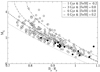 |
Fig. 1. Colour–magnitude diagram of the sample stars compared with the PARSEC isochrones (Bressan et al. 2012) projected into the Gaia eDR3 photometric system (Evans et al. 2018). The filled circles indicate stars with |
Only a few stars are located above the 6 Gyr ([Fe/H] = 0.2) isochrone. One of them exhibits a high activity level ( ) indicative of an age younger than 1 Gyr inconsistent with its position in the colour–magnitude diagram. This star is most likely a close binary in which rapid rotation and high activity are enforced by synchronisation of the rotation and orbital periods, due to tidal effects. Tidal interaction between main-sequence stars in binary systems is generally considered negligible if the orbital period is greater than ten days (Habets & Zwaan 1989). Binarity would thus have no significant effect on the age estimate derived from the chromospheric activity level of Sun-like stars older than 1 Gyr. Errors on their mass estimates would also have a limited effect since the evolution of their chromospheric activity index depends weakly on mass (Gondoin 2020).
Figure 2 shows the mean R′HK index distribution of the sample stars obtained by averaging the histograms of 1000 realisations of the R′HK index distribution assuming a Gaussian distribution around the mean values with the uncertainties provided in the AMBER-HARPS catalogue of  indices. The distribution shows an inactive peak near
  with an intermediate-activity shoulder in the 1.4−2.5 × 10⁻⁵
 range, and an active tail beyond
  ∼ 2.5 × 10⁻⁵.
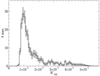 |
Fig. 2. Mean ⟨R′HK⟩ index distribution of all sample stars. The grey areas represent the ±1σ envelopes of the histograms of 1000 realisations of the distribution of R′HK indices of the sample stars assuming a Gaussian distribution around the mean measurement values with the uncertainties provided in the AMBER-HARPS catalogue of |

3. Age–activity relationship
Relationships between the age and the emission reversal in the cores of the Ca II H&K lines of late-type dwarfs have been derived in several studies (e.g. Skumanich 1972, Soderblom et al. 1991, Lachaume et al. 1999, Gondoin et al. 2012). The dependence of chromospheric activity on stellar mass, rotation and metallicity (Noyes et al. 1984; Mamajek & Hillenbrand 2008; Gray et al. 2006; Amard & Matt 2020) renders the calibration of an age–activity relationship difficult. In addition, the long-term evolution trend of activity indicators is blurred by the short-time variability of magnetic phenomena that includes the evolution of active regions and activity cycles.
In the past decade photometric surveys of open clusters have produced extensive rotation period measurements on many Sun-like stars of different ages (e.g. Gallet & Bouvier 2013). These surveys have shown that, beyond ∼600 Myr, the rotation rates of Sun-like stars with similar masses no longer depend on their initial rotation rate after circumstellar disc dispersion, but converge towards similar values (e.g. Barnes 2003; Meibom et al. 2009, 2011). Stellar age and mass then become the main parameters that determine the rotation and magnetic activity of 0.7–1.0 M⊙ stars with near-solar metallicity (Gondoin 2017, 2018).
Combining an activity versus Rossby number relationship (Mamajek & Hillenbrand 2008) with an empirical formulation of the convective turnover time (Wright et al. 2011) and rotation period measurements in intermediate-age open clusters (Meibom et al. 2015; Barnes et al. 2016; Curtis et al. 2019), Gondoin (2020) derived a model of the average  index evolution of Sun-like stars older than 1 Gyr. The author ran Monte Carlo simulations of
  index distributions among populations of nearby Sun-like stars assuming that their stellar birth function (i.e. the number of stars born per unit of mass and time) consists of several episodes of star formation occurring at different epochs. This model captures the main characteristics of a star formation event, namely a steep rise and a slow decline. It gives plausible age estimates for major star formation events and provide clues to the relative evolution of the thin disc and thick disc populations. However, the results inevitably depend on the a priori shape imposed on the age distribution.
An alternative approach without an a priori hypothesis on the star formation events consists in inverting the measured  index distribution calculating a chromospheric age for each individual star from its mass and average
  index. This can be achieved inverting the age–activity relationship used by Gondoin (2020).
For stars older than 1 Gyr with masses between 0.7 and 1.1 M⊙, and [Fe/H] between −0.2 and 0.2, the age t (in Gyr) of a star can be expressed as a function of its mean chromospheric activity index  and its mass M (in solar unit) as
with

where P0(M) is the rotation period of a 1 Gyr old dwarf with a mass between 0.7 and 1.1 M⊙ (Gondoin 2020),

and τc(M) its age-independent convective turnover time (Wright et al. 2011):

The determination of the mean chromospheric activity level of a star requires a large number of observations on a time span long enough to filter out short-term variability effects, including the evolution of active regions and activity cycles. The catalogue of Gomes da Silva et al. (2021) provides mean activity indices averaged on several measurements (up to a few hundred) distributed over a long time span (up to more than a decade). The number and precision of these data enable the ages of the sample stars to be closely constrained. The requirement on the number of measurements per star and on the length of the measurements period is alleviated if, instead of one star, we consider a group of coeval stars.
The precision of the age–activity relationship (Eq. (2)) can be estimated from the results of a spectroscopic survey of solar-type stars in the solar-age and solar-metallicity open cluster M67 (Giampapa et al. 1976). The authors found that 72%–80% of the solar analogues in this sample exhibit Ca II H&K strengths within the range of the modern solar cycle. This range was estimated to −4.955 < log ( < −4.832 from 1977 to 2008 by Mamajek & Hillenbrand (2008) from the data of Livingston et al. (2007). According to Eq. (2), the corresponding ages of the M67 solar mass stars is included between 4.6 and 3.5 Gyr, in agreement with the age of the cluster (4.1 ± 0.5 Gyr; Yadav et al. 2008). The precision of the inferred age–activity relationship would thus be about ±0.6 Gyr for these measurements of the
  indices of coeval stars.
Simulations of the age distributions of artificially created samples of coeval stars with the same masses, errors on masses, and errors on mean  indices as the sample stars show sharp peaks at the imposed ages with extended wings. The root mean square dispersion σage of the distributions range from 540 Myr for a 2 Gyr coeval sample to 890 Myr for a 6 Gyr sample. The ±σage interval around the peaks of the inverted distributions of the 2 Gyr (resp. 6 Gyr) test sample contain 98% (resp. 88%) of the sample stars. These results indicate that the accuracy of the age inversion method decays towards increasing ages due to the flattening of the activity versus age relationship, but remains better than 1 Gyr with a high confidence level.
4. Analysis
4.1. Age distribution of the sample stars
The upper graph in Fig. 3 shows the age distribution of all sample stars derived from their  indices using Eq. (2). The retrieved distribution is the average of 1000 simulations assuming Gaussian distributions of the mass and average
  index of each star around the average values provided in the AMBRE-HARPS catalogue of
  indices with the uncertainties given in the catalogue. The grey areas represent the ±1σ envelopes of the 1000 simulations.
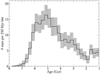 |
Fig. 3. Age distributions derived by inverting the |


The inferred age distribution shows a sharp rise in the number of stars per 250 Myr age bin between 7 and 6 Gyr ago. It reaches a maximum at an age of ∼5 Gyr. The distribution then shows a decaying trend of the number of stars per age bin until about 2 Gyr. This number rises again in the recent past, about 1.8 Gyr ago. However, the statistic is too low to assign a precise age to this recent event.
Extrapolating these results to the age distribution of Sun-like stars in the solar neighbourhood is reasonable if the stellar sample used in the present study is representative of the population of nearby 0.85−1.0 M⊙ dwarfs intended to be characterised. In the present case, selection effects could come from the HARPS spectrometer performance, from target selection criteria of the observation programmes that participated in the archive build up or from any criteria possibly used by the automated analysis pipelines to reject non-standard spectra.
In particular, the high spectral resolution of the HARPS spectrometer requires the observation of bright stars; the planet search programme may favour the observation of old inactive single G dwarfs and the pipeline analysis probably rejects non-standard spectra, such as those of binary stars, fast rotators, and very active stars. All together, these instrumental, programmatic, and analysis selection criteria are expected to favour single inactive G-type stars.
Following the approach of Henry et al. (1996), I classified the chromospheric activity levels of the sample stars into inactive ( ), active (
 ), and very active (
 ). Most sample stars (74%) have a low chromospheric activity level, an important fraction (23%) have a high activity level, and very few (∼3%) have a very high activity level.
For comparison, Henry et al. (1996) reported that in their sample of southern solar-type stars, the proportions of stars in the inactive, active, and very active chromospheric activity levels are 70.4%, 27.1 %, and 2.6% respectively. These proportions are 68%, 30.3%, and 1.7%, respectively among 0.85–1.0 M⊙ stars in a sample of single Sun-like stars (Gondoin 2020) obtained by cross-correlating the chromospheric activity catalogue of Boro-Saikia et al. (2018) with the PASTEL catalogue (Soubiran et al. 2016).
The distribution of activity level in the present sample is thus similar to that of the samples studied by Henry et al. (1996) and Gondoin (2020), but presents a slight deficit in active stars ( ). However, a two-sample Kolmogorov–Smirnov test applied to sub-samples of stars with
  extracted from the present sample and the sample of Gondoin (2020) does not invalidate the hypothesis that these two sub-samples originate from the same parent population. This supports the conclusion that the measured distribution of ages among the sample stars with
  is representative of the age distribution of nearby solar-type stars older than ∼1 Gyr.
4.2. Kinematics of the sample stars
Figure 4 shows the histograms of the space velocity components of the sample stars in the local standard of rest measured with the Gaia satellite. These components are expressed in a right-handed rectangular coordinate system (x, y, z) in which U, V, and W are positive in the direction of the Galactic centre, Galactic rotation, and the north Galactic pole, respectively.
 |
Fig. 4. Histograms of the U (left), V (middle), and W (right) velocity components of the sample stars in the local standard of rest measured with the Gaia satellite. |
Since the velocity histograms of the sample stars depart from Gaussian distributions, their origin from either the thin or thick disc of the Milky Way cannot be reliably estimated from their kinematics following the approach of Reddy et al. (2006), Bensby et al. (2003, 2004), and Mishenina et al. (2004). The Toomre diagram of the sample stars (Fig. 5) also does not show any clear-cut separation between populations of different origin in the disc.
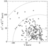 |
Fig. 5. Toomre diagram of the sample stars. The constant space velocity modulus ( |
The velocity components of the sample stars are plotted as a function of their chromospheric activity indices in Fig. 6. The dispersion of the radial velocities U of the sample stars increases towards a low activity level (i.e. towards old ages) both in the Galaxy centre and the anti-centre directions; a larger number of stars move in the anti-centre direction. The radial velocities of the less active stars are included between −120 and 80 km s−1.
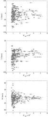 |
Fig. 6. U (top), V (middle), and W (bottom) velocity components of the sample stars in the local standard of rest measured with the Gaia satellite as a function of their chromospheric activity index. |
The dispersion of the tangential velocities V also increases towards a low activity level, but mainly towards negative velocities; in other words, more stars lag behind the local standard of rest at increasing age. The tangential velocities of the less active stars are included between −100 and 30 km s−1. The velocity dispersion of the sample stars perpendicular to the disc increases towards a low activity level (i.e. towards old ages). The dispersion of the vertical velocities W of the less active stars ranges between −70 and 60 km s−1.
The widths and asymmetries of the distributions of the U, V, and W velocity components of the sample stars in Figs. 4 and 6 are similar to those of the U, V, and W velocity histograms of a much larger sample of 74 281 nearby stars with a valid radial velocity extracted from the Gaia EDR3 catalogue (see Fig. 22 in Gaia Collaboration 2021).
Figure 7 shows the mean standard deviation of the U, V, and W velocity components of the sample stars in age bins of 20 stars as a function of the average age of the stars in each bin. In order to propagate the uncertainties on the mass and  measurements, I performed 1000 Gaussian Monte Carlo realisations of the age distribution of the stars using the corresponding uncertainties on the mass and
  index of each object provided in the AMBRE-HARPS catalogue. The vertical bars represent the ±1σ errors on the mean standard deviation of the velocity components.
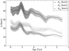 |
Fig. 7. Standard deviation of the U, V, and W velocity components of the sample stars in age bins of 20 stars as a function of the average age of the stars in those bins. The vertical bars represent the ±1σ errors on the mean standard deviation of the velocity components. The dot-dashed lines are best-fit power laws to the time evolution of the velocity component dispersions of all sample stars. |
The mean standard deviation of each velocity component increases towards old ages. Fitting power laws to these trends in the range 1.5 to 6 Gyr give exponents equal to 0.29, 0.46, and 0.63 for the U, V, and W velocity dispersions, respectively. These exponents are comparable to the values of 0.39, 0.40, and 0.53, respectively, derived from the Geneva–Copenhagen survey of the solar neighbourhood (Holmberg et al. 2009) that includes over 14 000 nearby F and G dwarfs with HIPPARCOS parallaxes, and accurate radial-velocity observations. Exponents of 0.31, 0.34, and 0.47 for the U, V, and W velocity dispersions, respectively, had been derived previously by Nordstrom et al. (2004) from the Geneva–Copenhagen survey, in agreement with Binney et al. (2000).
Although these power laws account for the increasing dispersion of the velocity components with age, all standard deviation curves show fluctuations around these best-fit evolution trends. In particular, fluctuations of the U and W velocity dispersions with an amplitude larger than 1σ above their best-fit power laws are observed at an age of ∼5.1 Gyr. Since the standard deviation measurements are performed with a constant number of stars per age bin, these maxima suggest that the dispersions of the U and W velocity components increases at the age of maximum star formation (see Fig. 3).
4.3. Iron abundance of the sample stars
The chemical compositions of the sample stars contain information on the formation process of the Milky Way disc. They encode the chemical properties of the interstellar medium at the epochs of their formation. Figure 8 shows the iron abundance of the sample stars as a function of their chromospheric activity index. The dispersion of the [Fe/H] abundance ratios is large at any activity level (i.e. at any age).
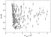 |
Fig. 8. Iron abundance of the sample stars as a function of their chromospheric activity index. |
Figure 9 shows the mean [Fe/H] abundance ratio of sample stars in age bins of 20 stars as a function of the average age of the stars in those bins. In order to propagate the uncertainties on the masses,  indices, and [Fe/H] ratios measurements, I performed 1000 Gaussian Monte Carlo realisations of the mean [Fe/H] distribution of the stars using the corresponding errors provided in the AMBRE-HARPS catalogue. The vertical bars represent the ±1σ errors on the average iron abundance. A circle indicates the iron abundance of the Sun at 4.57 Gyr (Bonanno et al. 2002).
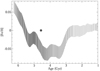 |
Fig. 9. Mean [Fe/H] abundance ratio of the sample stars in age bins of 20 stars as a function of the average age of the stars in those bins. The vertical bars represent the ±1σ errors on the mean [Fe/H] ratios. A circle indicates the iron abundance of the Sun. |
The mean iron abundance of the oldest sample stars is super-solar ([Fe/H] ∼ +0.05) at the beginning of star formation about 6 Gyr ago. It then decays and becomes significantly sub-solar ([Fe/H] < −0.05) between ∼4.6 and 3.3 Gyr ago. The mean iron abundance then rises continuously until slightly super-solar values ([Fe/H] ∼ +0.01) in the recent past.
This recent evolution is consistent with a monotonic metal enrichment history of the disc leading to element abundances increasing monotonically with time. In contrast, the co-existence of 4.6 to 3.3 Gyr old metal-poor stars with older but more metal-rich stars is clearly in conflict with a metal enrichment scenario. Although stellar migration effects cannot be excluded, the correlation between age and metallicity suggests a continuous dilution of the interstellar medium with the accretion of low-metallicity gas in the first 2–3 Gyr after the beginning of star formation about 7 Gyr ago.
A dip at around 4–5 Gyr in the age-metallicity relationship has been previously reported and discussed in a study of nearby solar-type stars with high-precision element abundances (Nissen et al. 2020) and in an analysis of a large spectroscopic survey of cool stars with a broad range of effective temperatures (Sahlholdt et al. 2022).
A drop in metallicity followed by a chemical enrichment episode with increasing [Fe/H] has also been identified at an earlier epoch in the age-metallicity relationship of the Galactic disc stars by Ciucǎ et al. (2023). The authors noted that this chemical evolution is similar to that induced by an early-epoch gas-rich merger identified in the Milky Way-like zoom-in cosmological simulation Auriga (Grand et al. 2020). These studies provide an insight into the effects onto the Galaxy of an event similar to the earlier Gaia-Enceladus-Sausage merger. In particular, they indicate that the low-metallicity gas from the gas-rich merger initially dilutes the metal content of the Galaxy. The merger then induces a significant formation of stars with a lower metallicity than those formed prior to the event.
5. Discussion
In the present study I address the origin of the chromospheric activity distribution of a sample of 222 Sun-like stars with −0.2 ≤ [Fe/H] ≤ 0.2 and masses between 0.85 and 1.0 M⊙ located within 65 pc from the Sun. The study sample is extracted from the catalogue of Gomes da Silva et al. (2021) that provides the mean chromospheric activity level of nearby cool stars obtained by averaging from a few to several thousand measurements of their chromospheric activity indices distributed on a time span from a few hours up to more than a decade. The atmospheric parameters including the iron abundances and the masses of the stars have been homogeneously determined by these authors. I retrieved their space velocity components from the catalogue of objects within 100 pc of the Sun produced from the Gaia Early Data Release 3 (Gaia Collaboration 2021).
I used an empirical age–activity relationship to infer the age distribution of the sample stars from their  indices. This relationship combines rotation period measurements in intermediate-age open clusters with a rotation-activity relationship. Late-type dwarfs experience a reduced braking efficiency and stalled spin-down between the ages of ∼670 Myr and ∼1 Gyr (Meibom et al. 2011, 2015; Rebull et al. 2017; Agueros et al. 2018; Curtis et al. 2019; Douglas et al. 2019). The decay of their
  index inferred from rotation period measurements in 1.0, 2.4, and 4.0 Gyr old clusters is thus slightly steeper than the activity evolution previously derived from the best fits to measured
  data in young (< 0.7 Gyr) open clusters, and in M67 (∼4 Gyr) or the Sun (e.g. Lorenzo-Oliveira et al. 2018; Zhang et al. 2019). Recent
  measurements (Booth et al. 2020) on solar-type stars with asteroseismeic ages that have masses lower than 1.1 M⊙, and near-solar metallicity (−0.2 ≤ [Fe/H] ≤ 0.2) supports the hypothesis of a continuously decreasing chromospheric activity until ∼7 Gyr ago.
The inferred age distribution of the sample stars shows a steep rise between 7 and 6 Gyr ago with a maximum ∼5 Gyr ago. The number of stars per 250 Myr age bin then decays until ∼2 Gyr and rises again in the recent past. A comparison of the colour–magnitude diagram of the sample stars (see Fig. 1) with the PARSEC isochrones (Bressan et al. 2012) confirms that most stars are located between the 1 Gyr ([Fe/H] = −0.2) and 6 Gyr ([Fe/H] = 0.2) isochrones. Since the distributions of activity levels and velocities among the sample stars are similar to those of previous samples of Sun-like stars, their derived age distribution can be compared with previous studies of the formation history of nearby dwarfs with origins at galactocentric distances similar to that of the region where the Sun was born.
The age–activity relationship used in the present study points to a dearth of near-solar metallicity stars older than 7 Gyr. This result is in line with the metallicity distribution function in the solar vicinity that is known to peak at solar metallicity, with most of its stars being younger than 7–8 Gyr (e.g. Haywood et al. 2019). This timeline is consistent with a quenching of star formation around the age of 8 Gyr that was derived by Snaith et al. (2015) from the Adibekyan et al. (2012) abundances and the Haywood et al. (2013) isochrone ages of solar-type stars. Mor et al. (2019) similarly report indications of a double-peaked star formation history with a minimum around 6 Gyr ago, from Gaia colour–magnitude diagrams. Other authors (Xiang & Rix 2022) found that the stellar age-metallicity distribution splits into two almost disjoint parts, separated at an age of 8 Gyr that may be interpreted as evidence of two episodes of accretion of gas onto the Galactic disc with quenching of star formation between them (Spitoni et al. 2023).
The question of how most nearby stars reached a metallicity [Fe/H] greater than −0.2 dex has long been known as the G-dwarf problem (van den Bergh 1962; Pagel & Patchett 1975). An answer can be provided if one considers that the solar vicinity did not evolve as a closed-box, but rather underwent gas flows, in particular gas infall (Greener et al. 2021; Matteucci 2021). Haywood et al. (2019) presented a scenario of the chemical enrichment of the solar neighbourhood that solves the G-dwarf problem. They suggested that the thick disc was formed from a turbulent gaseous disc that permitted a homogeneous distribution of metals, rather than a radially dependent distribution. This allowed the solar ring to be enriched to solar metallicity. According to these authors, this enrichment episode of the solar neighbourhood must have occurred after the thick disc reached solar metallicity, about 8–9 Gyr ago.
Various studies have reported a recent episode of star formation in the Milky Way. Using HIPPARCOS data in a sphere of 80 pc around the Sun and assuming a fixed initial mass function, Vergely et al. (2002) and Cignoni et al. (2006) derived maximum peaks of star formation 1.75−2 Gyr ago and 2−3 Gyr ago, respectively. Bernard (2017), in a tentative work using TGAS data, pointed towards the existence of a relative maximum of star formation also occurring 2–3 Gyr ago. Mor et al. (2019) found in Gaia DR2 data an imprint of a star formation burst 2–3 Gyr ago in the Galactic thin disc domain. Gondoin (2020) concluded that an important star formation episode that occurred ∼1.9–2.6 Gyr ago in the thin disc of the Milky Way can account for the distribution of magnetic activity among local G- and early K-type stars with a near-solar metallicity.
In view of the large timescale and of the large amount of mass involved in this recent star formation event, some authors (Cignoni et al. 2006; Mor et al. 2019) proposed that it is not intrinsic to the disc, but was produced by an external perturbation, possibly by a recent merger with a gas-rich satellite galaxy that could have started several Gyr ago. Ruiz-Lara et al. (2020) identified a number of peaks in the star formation rate within about 2 kpc obtained by colour–magnitude diagram fitting of Gaia data. These includes a recent peak ∼1.9 Gyr ago and an older more prominent peak located 5.7 Gyr ago, at ages similar to those of the youngest and oldest peaks found in the age distribution of the present stellar sample.
The authors interpret these peaks as being induced by the pericentre passages of the Sagittarius dwarf galaxy (Sgr) discovered by Ibata et al. (1994). This spheroidal galaxy is one of the closest and brightest satellites of the Milky Way. Having just passed pericentre, it is currently undergoing strong tidal disruption and is expected to completely dissolve over the next billion years (Vasiliev & Belokurov 2020; Vasiliev et al. 2021). Stars have been stripped from Sgr to form the Sagittarius stream, a pair of long tails that lead and trail Sgr. These wrap around the Milky Way in a plane roughly perpendicular to its disc (see e.g. Ibata et al. 2001; Majewski et al. 2003; Belokurov et al. 2006; Newberg et al. 2002).
The age distributions of the sample stars (see Fig. 3) shows that the number of stars involved in the oldest peak ∼5 Gyr ago is much larger than the number of stars involved in the youngest one. This indicates that the oldest event is by far the most important. A similar observation was noted by Ruiz-Lara et al. (2020).
The combined analysis of the kinematics data and age of the sample stars indicate that the dispersion of their space velocity components increases with age. A clear correlation between stellar age and velocity dispersion has been observed in the Milky Way (e.g. Nordstrom et al. 2004) and in other galaxies of the local group (Leaman et al. 2017) including M31 (Dorman et al. 2015; Bhattacharya et al. 2019), and M33 (Beasley et al. 2015). The classic explanation for this age-velocity relation is that stars always form in dynamically cold gas, but various gravitational scattering mechanisms steadily increase their random orbital energy with age (e.g. Wielen 1977; Lacey 1984).
The best-fit power laws to the velocity component dispersion of the sample stars have exponents similar to those derived from previous studies of the kinematics of nearby Sun-like stars (Nordstrom et al. 2004; Binney et al. 2000; Holmberg et al. 2009; Yu & Liu 2018). This supports the view that the present day velocity dispersion of the metal-rich population of nearby stars is consistent with heating mechanisms via scattering processes possibly induced by spiral arms and giant molecular clouds (GMCs). Sharma et al. (2021) point out that the observed dispersion is the end result of the heating history of stellar populations born at different times. Its interpretation is thus complex, in particular due to the higher gas fraction in the early Galactic disc that change the contribution of GMCs scattering over time.
Although power laws account for a continuous increase in the stars’ velocity dispersion with age, fluctuations above the best-fit power laws show an increase in the dispersions of the U and W stellar velocity components at the age of maximum star formation (see Fig. 7). This behaviour suggests alternative explanations according to which old nearby stars are born dynamically hotter due to a more active galaxy merger phase (Toth & Ostriker 1992; Quinn et al. 1993; Brook et al. 2004; Martig et al. 2014; Hu & Sijacki 2018; Buck et al. 2020), a higher gravitational turbulence if the disc was more gas rich (Bournaud et al. 2009), or a higher star formation rate (Lehnert et al. 2014). The disc would then settle and become progressively cooler as the star forming gas cools with time.
These explanations are consistent with a scenario where the steep rise in the age distribution of nearby Sun-like stars around 7−6 Gyr and their increased velocity dispersion is related to an external perturbation induced by a merger with a gas-rich satellite galaxy. The date of this event is compatible with that of the first close pericentric passage of the Sgr galaxy ∼6.5 Gyr ago. Stars younger than 5 Gyr would show a decaying trend of the dispersion of their velocity components as the disc becomes progressively cooler and the star forming gas cools with time. Subsequent dynamical heating by spiral arms, and galactic molecular clouds could have slowed down this cooling process.
According to this scenario, the Sgr galaxy would have been significantly stripped from its gas in this first encounter with the Milky Way disc, thus explaining the lower amplitude of the more recent formation event ∼1.8 Gyr ago. Dynamical modelling of the disruption of Sgr estimate the present-day mass of the Sgr remnant to 2.5 × 10⁸ M⊙ (Law & Majewski 2010) and 4 × 10⁸ M⊙ (Vasiliev & Belokurov 2020). However, a much higher mass of the Sgr progenitor (> 4–6 × 10¹⁰ M⊙) at its first infall has been proposed in a number of different studies (e.g. Jiang & Binney 2000; Read & Erkal 2019; Dillamore et al. 2022).
In order to account for such a massive Sgr precursor and to reproduce the star formation burst at its first infall 6 Gyr ago, hydrodynamical simulations (Annem & Khoperskov 2022) require a close pericentric passage (< 20 kpc) with subsequent substantial mass loss of the Sgr precursor.
The metallicity distribution function in the core of Sgr dSph but outside the nuclear region best approximates the conditions near the centre of the Sgr progenitor (Minelli et al. 2023). According to these authors, it is characterised by a peak at [Fe/H] ∼ −0.5 plus a wide and weak tail reaching [Fe/H] ≤ −2.0. Soon after the first pericentric passage, the gas infall from the satellite galaxy could have diluted the initially super-solar metallicity of the Milky Way outer disc. The event would have triggered the subsequent formation of a substantial amount of stars with a decreasing mean metallicity over an extended period of time.
This scenario would explain the early decay of the mean [Fe/H] ratio of the sample stars from a slightly super-solar value ∼6 Gyr ago to a slightly sub-solar value of ∼4 Gyr ago. A continuous metal enrichment of the disc would have progressively compensated the decaying infall of low-metallicity gas leading to an increase in the mean stellar metallicity of the solar neighbourhood in the last 4 Gyr. This scenario can also account for the observed chrono-chemodynamical structure of the outer disc of the Milky Way beyond the solar neighbourhood (Das et al. 2023).
6. Summary
In this study I addressed the formation history of nearby 0.85−1.0 M⊙ stars with −0.2 ≤ [Fe/H] ≤ +0.2 using the emission reversal in the cores of their Ca II H&K Fraunhofer lines as an age indicator. An empirical age–activity relationship derived from stellar rotation period measurements in intermediate-age open clusters was used to infer their age distribution and to estimate the evolution of their velocity components and mean metallicity.
The result indicates a steep rise in the formation of Sun-like stars in the solar neighbourhood between 7 and 6 Gyr ago with a maximum ∼5 Gyr ago. The star formation then decays until ∼2 Gyr and increases again in the recent past at ∼1.8 Gyr.
This timeline is consistent with a formation model of the Galaxy disc in two episodes of gas accretion, with a quenching of star formation between them about 8 Gyr ago. In the second episode of gas accretion, the steep rise in the age distribution of nearby Sun-like stars around 7−6 Gyr ago could be related to an external perturbation induced by a first close pericentric passage of the Sgr galaxy ∼6.5 Gyr ago.
The Sgr galaxy would have been significantly stripped from its gas in this first encounter with the Milky Way disc, thus explaining the lower amplitude of the more recent formation event ∼1.8 Gyr ago. The turbulence induced during the initial encounter may be partly responsible for the increased dispersion of the U and W stellar velocity components around the age of maximum star formation.
The gas infall from the satellite galaxy onto the Milky Way disc over an extended period of time would have first diluted the mean stellar metallicity after the first pericentric passage. This would explain the decay of the mean iron abundance of the sample stars from the first encounter until the age of ∼4 Gyr. A continuous metal enrichment of the disc would have then progressively compensated the decaying infall of low-metallicity gas leading to an increase in the mean stellar metallicity from ∼4 Gyr ago until the recent past.
Acknowledgments
This research has made use of the VizieR catalogue access tool, CDS, Strasbourg, France and of the NASA’s Astrophysics Data System Bibliographic Services. This work has made use of data from the European Space Agency (ESA) mission Gaia (https://www.cosmos.esa.int/gaia), processed by the Gaia Data Processing and Analysis Consortium (DPAC, https://www.cosmos.esa.int/web/gaia/dpac/consortium). Funding for the DPAC has been provided by national institutions, in particular the institutions participating in the Gaia Multilateral Agreement. I am grateful to the anonymous referee for the helpful comments that allowed me to improve the paper.
References
- Adibekyan, V. Zh., Sousa, S. G., Santos, N. C., et al. 2012, A&A, 545, A32 [NASA ADS] [CrossRef] [EDP Sciences] [Google Scholar]
- Agueros, M. A., Bowsher, E. C., Bochanski, J. J., et al. 2018, ApJ, 862, 33 [NASA ADS] [CrossRef] [Google Scholar]
- Amard, L., & Matt, S. P. 2020, ApJ, 889, 108 [Google Scholar]
- Anders, F., Chiappini, C., Santiago, B. X., et al. 2014, A&A, 564, A115 [NASA ADS] [CrossRef] [EDP Sciences] [Google Scholar]
- Annem, B., & Khoperskov, S. 2022, MNRAS, submitted [arXiv:2210.17054] [Google Scholar]
- Baliunas, S. L., Donahue, R. A., Soon, W. H., et al. 1995, ApJ, 438, 269 [Google Scholar]
- Barnes, S. A. 2003, ApJ, 586, 464 [Google Scholar]
- Barnes, S. A., Weingrill, J., Fritzweski, D., et al. 2016, ApJ, 823, 16 [CrossRef] [Google Scholar]
- Barry, D. C. 1988, ApJ, 334, 436 [NASA ADS] [CrossRef] [Google Scholar]
- Beasley, M. A., San Roman, I., Gallart, C., et al. 2015, MNRAS, 451, 3400 [NASA ADS] [CrossRef] [Google Scholar]
- Belokurov, V., Zucker, D. B., Evans, N. W., et al. 2006, ApJ, 642, L137 [Google Scholar]
- Bensby, T., Feltzing, S., & Lundström, I. 2003, A&A, 410, 527 [CrossRef] [EDP Sciences] [Google Scholar]
- Bensby, T., Feltzing, S., & Lundström, I. 2004, A&A, 421, 969 [NASA ADS] [CrossRef] [EDP Sciences] [Google Scholar]
- Bernard, E. J. 2017, Reconstructing the Star Formation History of the Solar Neighbourhood with Gaia. Proceedings of the International Astronomical Union, 13, 158 [Google Scholar]
- Bhattacharya, S., Arnaboldi, M., Caldwell, N., et al. 2019, A&A, 631, A56 [NASA ADS] [CrossRef] [EDP Sciences] [Google Scholar]
- Binney, J., Dehnen, W., & Bertelli, G. 2000, MNRAS, 318, 658 [NASA ADS] [CrossRef] [Google Scholar]
- Bland-Hauthorn, J., & Ortwin, G. 2016, ARA&A, 54, 529 [NASA ADS] [CrossRef] [Google Scholar]
- Bonanno, A., Schlattl, H., & Paterno, L. 2002, A&A, 390, 1115 [NASA ADS] [CrossRef] [EDP Sciences] [Google Scholar]
- Booth, R. S., Poppenhaeger, K., Watson, C. A., et al. 2020, MNRAS, 491, 455 [NASA ADS] [CrossRef] [Google Scholar]
- Boro-Saikia, S., Marvin, C. J., Jeffers, S. V., et al. 2018, A&A, 616, A108 [NASA ADS] [CrossRef] [EDP Sciences] [Google Scholar]
- Bournaud, F., Elmegreen, B. G., & Martig, M. 2009, ApJ, 707, L1 [Google Scholar]
- Bressan, A., Marigo, P., Girardi, L., et al. 2012, MNRAS, 427, 127 [NASA ADS] [CrossRef] [Google Scholar]
- Brook, C. B., Kawata, D., Gibson, B. K., et al. 2004, ApJ, 612, 894 [NASA ADS] [CrossRef] [Google Scholar]
- Buck, T., Obreja, A., Maccio, A. V., et al. 2020, MNRAS, 491, 3461 [Google Scholar]
- Cignoni, M., Degl’Innocenti, S., Prada Moroni, P. G., et al. 2006, A&A, 459, 783 [NASA ADS] [CrossRef] [EDP Sciences] [Google Scholar]
- Ciucǎ, I., Kawata, D., Ting, Y.-S., et al. 2023, MNRAS, in press, https://doi.org/10.1093/mnrasl/slad033 [Google Scholar]
- Curtis, J. L., Agueros, M. A., Douglas, S. T., et al. 2019, ApJ, 879, 49 [NASA ADS] [CrossRef] [Google Scholar]
- Das, P., Huang, Y., Ciuca, I., & Fragkoudi, F. 2023, MNRAS, submitted [arXiv:2305.07426] [Google Scholar]
- da Silva, L., Girardi, L., Pasquini, L., et al. 2006, A&A, 458, 609 [NASA ADS] [CrossRef] [EDP Sciences] [Google Scholar]
- de Laverny, P., Recio-Blanco, A., Worley, C. C., et al. 2013, The Messenger, 153, 8 [Google Scholar]
- Dillamore, A. M., Belokurov, V., Evans, N. W., et al. 2022, MNRAS, 516, 1685 [NASA ADS] [CrossRef] [Google Scholar]
- Dorman, C. E., Guhathakurta, P., Seth, A. C., et al. 2015, ApJ, 803, 24 [Google Scholar]
- Douglas, S. T., Curtis, J. L., Agueros, M. A., et al. 2019, ApJ, 879, 100 [NASA ADS] [CrossRef] [Google Scholar]
- Duncan, D. K., Vaughan, A. H., Wilson, O. C., et al. 1991, ApJS, 76, 383 [Google Scholar]
- Esteban, C., Mendez-Delgado, J. E., Garcia-Rojas, J., et al. 2022, ApJ, 931, 92 [NASA ADS] [CrossRef] [Google Scholar]
- Evans, D. W., Riello, W., De Angeli, F., et al. 2018, A&A, 616, A4 [NASA ADS] [CrossRef] [EDP Sciences] [Google Scholar]
- Fantin, N. J., Cote, P., McConnachie, A. W., et al. 2019, ApJ, 887, 148 [NASA ADS] [CrossRef] [Google Scholar]
- Gaia Collaboration (Babusiaux, C., et al.) 2018, A&A, 616, A10 [NASA ADS] [CrossRef] [EDP Sciences] [Google Scholar]
- Gaia Collaboration (Smart, R. L., et al.) 2021, A&A, 649, A6 [EDP Sciences] [Google Scholar]
- Gallet, F., & Bouvier, J. 2013, A&A, 556, A36 [NASA ADS] [CrossRef] [EDP Sciences] [Google Scholar]
- Giampapa, M. S., Hall, J. C., Radick, R. R., et al. 1976, ApJ, 651, 444 [Google Scholar]
- Gomes da Silva, J., Santos, N. C., Adibekyan, V., et al. 2021, A&A, 646, A77 [NASA ADS] [CrossRef] [EDP Sciences] [Google Scholar]
- Gondoin, P. 2017, A&A, 599, A122 [NASA ADS] [CrossRef] [EDP Sciences] [Google Scholar]
- Gondoin, P. 2018, A&A, 616, A154 [NASA ADS] [CrossRef] [EDP Sciences] [Google Scholar]
- Gondoin, P. 2020, A&A, 641, A110 [NASA ADS] [CrossRef] [EDP Sciences] [Google Scholar]
- Gondoin, P., Gandolfi, D., Fridlund, M., et al. 2012, A&A, 548, A15 [NASA ADS] [CrossRef] [EDP Sciences] [Google Scholar]
- Grand, R. J. J., Kawata, D., Belokurov, V., et al. 2020, MNRAS, 497, 1603 [NASA ADS] [CrossRef] [Google Scholar]
- Gray, R. O., Corbally, C. J., Garrison, R. F., et al. 2006, AJ, 132, 161 [Google Scholar]
- Greener, M. J., Merrifield, M., Aragon-Salamanca, A., et al. 2021, MNRAS, 502, L95 [NASA ADS] [CrossRef] [Google Scholar]
- Habets, G. M. H. J., & Zwaan, C. 1989, A&A, 211, 56 [NASA ADS] [Google Scholar]
- Hall, J. C. 2008, Liv. Rev. Sol. Phys., 5, 2 [Google Scholar]
- Hayden, M. R., Holtzman, J. A., Bovy, J., et al. 2014, AJ, 147, 116 [NASA ADS] [CrossRef] [Google Scholar]
- Hayden, M. R., Bland-Hawthorn, J., Sharma, S., et al. 2020, MNRAS, 493, 2952 [Google Scholar]
- Haywood, M., Di Matteo, P., Lehnert, M. D., et al. 2013, A&A, 560, A109 [NASA ADS] [CrossRef] [EDP Sciences] [Google Scholar]
- Haywood, M., Snaith, O., Lehnert, M. D., et al. 2019, A&A, 625, A105 [NASA ADS] [CrossRef] [EDP Sciences] [Google Scholar]
- Helmi, A. 2020, ARA&A, 58, 205 [Google Scholar]
- Henry, T. J., Soderblom, D. R., Donahue, R. A., et al. 1996, AJ, 111, 439 [NASA ADS] [CrossRef] [Google Scholar]
- Holmberg, J., Nordstrom, B., & Andersen, J. 2009, A&A, 501, 941 [NASA ADS] [CrossRef] [EDP Sciences] [Google Scholar]
- Hu, S., & Sijacki, D. 2018, MNRAS, 478, 1576 [NASA ADS] [CrossRef] [Google Scholar]
- Ibata, R. A., Gilmore, G., & Irwin, M. J. 1994, Nature, 370, 194 [Google Scholar]
- Ibata, R., Irwin, M., Lewis, G. F., et al. 2001, ApJ, 547, L133 [NASA ADS] [CrossRef] [Google Scholar]
- Jiang, I.-G., & Binney, J. 2000, MNRAS, 314, 468 [Google Scholar]
- Lacey, C. G. 1984, MNRAS, 208, 687 [NASA ADS] [CrossRef] [Google Scholar]
- Lachaume, R., Dominik, C., & Habing, H. J. 1999, A&A, 348, 897 [NASA ADS] [Google Scholar]
- Lallement, R., Welsh, B. Y., Vergely, J. L., et al. 2003, A&A, 411, 447 [NASA ADS] [CrossRef] [EDP Sciences] [Google Scholar]
- Law, D. R., & Majewski, S. R. 2010, ApJ, 718, 1128 [Google Scholar]
- Leaman, R., Mendel, J. T., Wisnioski, E., et al. 2017, MNRAS, 472, 1879 [Google Scholar]
- Lehnert, M. D., Di Matteo, P., Haywood, M., et al. 2014, ApJ, 789, L30 [NASA ADS] [CrossRef] [Google Scholar]
- Lemasle, B., Francois, P., Genovali, K., et al. 2013, A&A, 558, A31 [NASA ADS] [CrossRef] [EDP Sciences] [Google Scholar]
- Linsky, J. L., Worden, S. P., McClintock, W., et al. 1979, ApJS, 41, 47 [NASA ADS] [CrossRef] [Google Scholar]
- Livingston, W., Wallace, L., White, O. R., et al. 2007, ApJ, 657, 1137 [CrossRef] [Google Scholar]
- Lorenzo-Oliveira, D., Freitas, F. C., Melendez, J., et al. 2018, A&A, 619, A73 [NASA ADS] [CrossRef] [EDP Sciences] [Google Scholar]
- Luck, R. E., & Lambert, D. L. 2011, AJ, 142, 136 [Google Scholar]
- Majewski, S. R., Skrutskie, M. F., Weinberg, M. D., et al. 2003, ApJ., 599, 1082 [NASA ADS] [CrossRef] [Google Scholar]
- Malmquist, G. 1922, Arkiv för Matematik, Astronomi och Fysik., 16, 1 [Google Scholar]
- Malmquist, G. 1925, Arkiv för Matematik, Astronomi och Fysik, 19, 1 [Google Scholar]
- Mamajek, E. E., & Hillenbrand, L. A. 2008, ApJ, 687, 1264 [Google Scholar]
- Martig, M., Minchev, I., & Flynn, C. 2014, MNRAS, 443, 2452 [Google Scholar]
- Matteucci, F. 2021, A&ARv, 29, 5 [NASA ADS] [CrossRef] [Google Scholar]
- Meibom, S., Mathieu, R. D., & Stassun, K. G. 2009, ApJ, 695, 679 [Google Scholar]
- Meibom, S., Matthieu, R. D., Stassun, K. G., et al. 2011, ApJ, 733, 115 [NASA ADS] [CrossRef] [Google Scholar]
- Meibom, S., Barnes, S. A., Platais, I., et al. 2015, Nature, 517, 589 [Google Scholar]
- Mestel, L., & Spruit, H. C. 1987, MNRAS, 228, 57 [NASA ADS] [CrossRef] [Google Scholar]
- Minelli, A., Bellazzini, M., Mucciarelli, A., et al. 2023, A&A, 669, A54 [NASA ADS] [CrossRef] [EDP Sciences] [Google Scholar]
- Mishenina, T. V., Soubiran, C., Kovtyukh, V. V., et al. 2004, A&A, 418, 551 [NASA ADS] [CrossRef] [EDP Sciences] [Google Scholar]
- Mowlavi, N., Eggenberger, P., Meynet, G., et al. 2012, A&A, 541, A41 [NASA ADS] [CrossRef] [EDP Sciences] [Google Scholar]
- Mor, R., Robin, A. C., Figueras, F., et al. 2019, A&A, 624, L1 [NASA ADS] [CrossRef] [EDP Sciences] [Google Scholar]
- Newberg, H. J., Yanny, B., Rockosi, C., et al. 2002, ApJ, 569, 245 [Google Scholar]
- Nissen, P. E., Christensen-Dalsgaard, J., Mosumgaard, J. R., et al. 2020, A&A, 640, A81 [NASA ADS] [CrossRef] [EDP Sciences] [Google Scholar]
- Nordstrom, B., Mayor, M., Andersen, J., et al. 2004, A&A, 418, 989 [NASA ADS] [CrossRef] [EDP Sciences] [Google Scholar]
- Noyes, R. W., Hartmann, L. W., Baliunas, S. L., et al. 1984, ApJ, 279, 763 [NASA ADS] [CrossRef] [Google Scholar]
- Pagel, B. E. J., & Patchett, B. E. 1975, MNRAS, 172, 13 [NASA ADS] [CrossRef] [Google Scholar]
- Pallavicini, R., Golub, L., Rosner, R., et al. 1981, ApJ, 248, 279 [NASA ADS] [CrossRef] [Google Scholar]
- Quinn, P. J., Hernquist, L., & Fullagar, D. P. 1993, ApJ, 403, 74 [Google Scholar]
- Read, J. I., & Erkal, D. 2019, MNRAS, 487, 5799 [Google Scholar]
- Rebull, L. M., Stauffer, J. R., Hillenbrand, L. A., et al. 2017, ApJ, 839, 92 [Google Scholar]
- Reddy, B. E., Lambert, D. L., & Prieto, C. A. 2006, MNRAS, 367, 1329 [NASA ADS] [CrossRef] [Google Scholar]
- Rocha-Pinto, H. J., Scalo, J., Maciel, W. J., et al. 2000, ApJ, 531, L115 [NASA ADS] [CrossRef] [Google Scholar]
- Ruiz-Lara, T., Gallart, C., Bernard, E. J., et al. 2020, Nat. Astron., 4, 265 [Google Scholar]
- Sahlholdt, C. L., Feltzing, S., & Feuillet, D. K. 2022, MNRAS, 510, 4669 [NASA ADS] [CrossRef] [Google Scholar]
- Sharma, S., Hayden, M. R., Bland-Hawthorn, J., et al. 2021, MNRAS, 506, 1761 [NASA ADS] [CrossRef] [Google Scholar]
- Skumanich, A. 1972, ApJ, 171, 565 [Google Scholar]
- Snaith, O., Haywood, M., Di Matteo, P., et al. 2015, A&A, 578, A87 [NASA ADS] [CrossRef] [EDP Sciences] [Google Scholar]
- Soderblom, D. R., Duncan, D. K., & Johnson, D. R. H. 1991, ApJ, 375, 722 [NASA ADS] [CrossRef] [Google Scholar]
- Soubiran, C., Le Campion, J.-F., Brouillet, N., et al. 2016, A&A, 591, A118 [NASA ADS] [CrossRef] [EDP Sciences] [Google Scholar]
- Spitoni, E., Recio-Blanco, A., de Laverny, P., et al. 2023, A&A, 670, A109 [NASA ADS] [CrossRef] [EDP Sciences] [Google Scholar]
- Toth, G., & Ostriker, J. P. 1992, ApJ, 389, 5 [NASA ADS] [CrossRef] [Google Scholar]
- van den Bergh, S. 1962, AJ, 67, 486 [Google Scholar]
- Vasiliev, E., & Belokurov, V. 2020, MNRAS, 497, 4162 [Google Scholar]
- Vasiliev, E., Belokurov, V., & Erkal, D. 2021, MNRAS, 501, 2279 [NASA ADS] [CrossRef] [Google Scholar]
- Vaughan, A. H., & Preston, G. W. 1980, PASP, 92, 385 [Google Scholar]
- Vergely, J.-L., Köppen, J., Egret, D., et al. 2002, A&A, 390, 917 [NASA ADS] [CrossRef] [EDP Sciences] [Google Scholar]
- Vidotto, A. A. 2021, Living Rev. Sol. Phys., 18, 3 [NASA ADS] [Google Scholar]
- Wielen, R. 1974, in Highlights of Astronomy, eds. G. Gontopoulos, & G. Gontopoulos (Dordrecht: Reidel), 3, 395 [NASA ADS] [CrossRef] [Google Scholar]
- Wielen, R. 1977, A&A, 60, 263 [NASA ADS] [Google Scholar]
- Wilson, O. C. 1968, ApJ, 153, 221 [Google Scholar]
- Wright, N. J., Drake, J. J., Mamajek, E. E., & Henry, G. W. 2011, ApJ, 743, 48 [Google Scholar]
- Xiang, M., & Rix, H.-W. 2022, Nature, 603, 599 [NASA ADS] [CrossRef] [Google Scholar]
- Yadav, R. K. S., Bedin, L. R., Piotto, G., et al. 2008, A&A, 484, 609 [NASA ADS] [CrossRef] [EDP Sciences] [Google Scholar]
- Yu, J., & Liu, C. 2018, MNRAS, 475, 1093 [Google Scholar]
- Zhang, J., Zhao, J., Oswalt, T. D., et al. 2019, ApJ, 887, 84 [NASA ADS] [CrossRef] [Google Scholar]
All Figures
|
Fig. 1. Colour–magnitude diagram of the sample stars compared with the PARSEC isochrones (Bressan et al. 2012) projected into the Gaia eDR3 photometric system (Evans et al. 2018). The filled circles indicate stars with |
| In the text | |
|
Fig. 2. Mean ⟨R′HK⟩ index distribution of all sample stars. The grey areas represent the ±1σ envelopes of the histograms of 1000 realisations of the distribution of R′HK indices of the sample stars assuming a Gaussian distribution around the mean measurement values with the uncertainties provided in the AMBER-HARPS catalogue of |
| In the text | |
|
Fig. 3. Age distributions derived by inverting the |
| In the text | |
|
Fig. 4. Histograms of the U (left), V (middle), and W (right) velocity components of the sample stars in the local standard of rest measured with the Gaia satellite. |
| In the text | |
|
Fig. 5. Toomre diagram of the sample stars. The constant space velocity modulus ( |
| In the text | |
|
Fig. 6. U (top), V (middle), and W (bottom) velocity components of the sample stars in the local standard of rest measured with the Gaia satellite as a function of their chromospheric activity index. |
| In the text | |
|
Fig. 7. Standard deviation of the U, V, and W velocity components of the sample stars in age bins of 20 stars as a function of the average age of the stars in those bins. The vertical bars represent the ±1σ errors on the mean standard deviation of the velocity components. The dot-dashed lines are best-fit power laws to the time evolution of the velocity component dispersions of all sample stars. |
| In the text | |
|
Fig. 8. Iron abundance of the sample stars as a function of their chromospheric activity index. |
| In the text | |
|
Fig. 9. Mean [Fe/H] abundance ratio of the sample stars in age bins of 20 stars as a function of the average age of the stars in those bins. The vertical bars represent the ±1σ errors on the mean [Fe/H] ratios. A circle indicates the iron abundance of the Sun. |
| In the text | |
Current usage metrics show cumulative count of Article Views (full-text article views including HTML views, PDF and ePub downloads, according to the available data) and Abstracts Views on Vision4Press platform.
Data correspond to usage on the plateform after 2015. The current usage metrics is available 48-96 hours after online publication and is updated daily on week days.
Initial download of the metrics may take a while.