| Issue |
A&A
Volume 678, October 2023
|
|
|---|---|---|
| Article Number | A40 | |
| Number of page(s) | 14 | |
| Section | The Sun and the Heliosphere | |
| DOI | https://doi.org/10.1051/0004-6361/202346689 | |
| Published online | 29 September 2023 | |
Coronal energy release by MHD avalanches
Effects on a structured, active region, multi-threaded coronal loop
1
Dipartimento di Fisica & Chimica, Università di Palermo, Piazza del Parlamento 1, 90134 Palermo, Italy
e-mail: gabriele.cozzo@unipa.it
2
School of Mathematics and Statistics, University of St Andrews, St Andrews, Fife KY16 9SS, UK
e-mail: jr93@st-andrews.ac.uk
3
INAF – Osservatorio Astronomico di Palermo, Piazza del Parlamento 1, 90134 Palermo, Italy
e-mail: paolo.pagano@inaf.it
Received:
18
April
2023
Accepted:
8
June
2023
Context. A possible key element for large-scale energy release in the solar corona is a magnetohydrodynamic (MHD) kink instability in a single twisted magnetic flux tube. An initial helical current sheet progressively fragments in a turbulent way into smaller-scale sheets. Dissipation of these sheets is similar to a nanoflare storm. Since the loop expands in the radial direction during the relaxation process, an unstable loop can disrupt nearby stable loops and trigger an MHD avalanche.
Aims. Exploratory investigations have been conducted in previous works with relatively simplified loop configurations. In this work, we address a more realistic environment that comprehensively accounts for most of the physical effects involved in a stratified atmosphere typical of an active region. The questions we investigate are whether the avalanche process will be triggered, with what timescales, and how will it develop as compared with the original, simpler approach.
Methods. We used three-dimensional MHD simulations to describe the interaction of magnetic flux tubes, which have a stratified atmosphere with chromospheric layers, a thin transition region to the corona, and a related transition from high-β to dlow-β regions. The model also includes the effects of thermal conduction and of optically thin radiation.
Results. Our simulations address the case where one flux tube amongst a few is twisted at the footpoints faster than its neighbours. We show that this flux tube becomes kink unstable first in conditions in agreement with those predicted by analytical models. It then rapidly affects nearby stable tubes, instigating significant magnetic reconnection and dissipation of energy as heat. In turn, the heating brings about chromospheric evaporation as the temperature rises up to about 107 K, close to microflare observations.
Conclusions. This work confirms, in more realistic conditions, that avalanches are a viable mechanism for the storing and release of magnetic energy in plasma confined in closed coronal loops as a result of photospheric motions.
Key words: plasmas / magnetohydrodynamics (MHD) / Sun: corona / Sun: magnetic fields
© The Authors 2023
 Open Access article, published by EDP Sciences, under the terms of the Creative Commons Attribution License (https://creativecommons.org/licenses/by/4.0), which permits unrestricted use, distribution, and reproduction in any medium, provided the original work is properly cited.
This article is published in open access under the Subscribe to Open model. Subscribe to A&A to support open access publication.
1. Introduction
The magnetic activity in the solar corona consists of a wide range of events, reflecting the dynamic nature of the environment. The role of the magnetic field as the dominant reservoir of energy that may heat the corona to millions of kelvin is now widely accepted. Moreover, it is now clear that the ‘coronal heating problem’ must address the whole solar atmosphere as a highly coupled system (Parnell & De Moortel 2012); that is, the solar corona must not be treated as an isolated environment, but as an energetically open system with continuous interactions with the underlying layers (i.e. the chromosphere and photosphere). However, the nature of the mechanisms that might lead the magnetic field to supply energy to the corona is still highly debated. Although several processes have been proposed in recent decades, it is still unclear how they interact to produce the complex behaviour of the solar atmosphere. For instance, photospheric observations show a very clumpy magnetic field organized into clusters of elemental flux tubes (Gomez et al. 1993). Above that, the bright corona consists of arch-like magnetic structures called coronal loops that connect regions with different polarity (Vaiana et al. 1973; Reale 2014). The loops are, in turn, structured into thinner magnetic strands that reflect the underlying granular pattern. Tangling and twisting of the coronal magnetic strands cannot be avoided, according to photospheric observations. The field must therefore reconnect in order to prevent an infinite build-up of stress. This inevitably produces plasma heating (Parker 1972; Klimchuk 2015). Investigating coronal loops is of fundamental importance to understanding the key physical aspects of several heating mechanisms based on magnetic stress.
Coronal loops are generally organized into clusters of thin, twisted threads (also called ‘strands’) that follow the same behaviour. Nevertheless, as coronal loops commonly exhibit strong magnetic fields of the order of 10 G or more (Yang et al. 2020; Long et al. 2017; Brooks et al. 2021), and the coronal plasma is nearly ideal, transport of matter across the field is strongly inhibited. In other words, the magnetic field confines the plasma within the flux tubes. Moreover, since magnetic forces are much stronger than gravity in the corona, the latter will effectively act only along the field lines. Tenuous plasma is strongly funnelled along the field lines and also thermally isolated from the surroundings (Rosner et al. 1978; Vesecky et al. 1979). Coronal loops are anchored to the underlying chromosphere and, a little further down, to the photospheric layer, where the plasma β parameter exceeds unity by a few orders of magnitude. There, the so-called footpoints of the loop are dragged by photospheric plasma motion, which, in turn, might be highly irregular and turbulent. The typical strength of the magnetic field in the photosphere has been found to be hundreds of Gauss in active regions and sunspots (Ishikawa et al. 2021). Higher in the corona, the plasma pressure decreases, the flux tube progressively expands, and the magnetic field strength decreases while the magnetic flux is conserved. The greatest expansion rate is expected across the thin transition region separating the chromosphere from the overlying corona (Gabriel 1976). There, the temperature rapidly increases from thousands to millions of kelvin and, consequently, the pressure scale-height increases by several orders of magnitude.
The solar corona may be heated both by dissipation of stored magnetic stresses (DC heating) and by the damping of waves (AC heating; Parnell & De Moortel 2012; Zirker 1993). In particular, DC heating must involve both storage and impulsive release of magnetic energy. In solar active regions, the energy is presumably stored over timescales longer than an Alfvén time. A reasonable general assumption is that the magnetic field evolves quasi-statically through a sequence of equilibria, slowly changing because the coronal footpoints are rigidly line-tied to the low-beta photospheric plasma. As the coronal field moves through these equilibria, energy is injected by the motions and is then stored. Observations and numerical experiments provide evidence that the evolution of coronal loops is strongly influenced by photospheric motions (Chen et al. 2021). The coronal magnetic field must be driven towards a stressed state, which will be a non-potential configuration. For instance, footpoint rotation may lead the magnetic structure to twist and gain magnetic energy. While magnetic energy is stored, the flux tube could potentially be subject to strong stresses that may eventually trigger fast magnetohydrodynamic instabilities, such as the kink instability (Hood et al. 2009) or the tearing mode instability (Del Zanna et al. 2016), or lead to long-lasting Ohmic heating (Klimchuk 2006). The details of this conversion, for instance whether it is continuous or by sequences of pulses (nanoflares), are still under investigation. Another outstanding issue is the spatial distribution of the heating, which may reveal a filamentary structure on coronal loops.
Heating and brightening of coronal loops may occur as a ‘storm’ of impulsive events (Klimchuk 2009; Viall & Klimchuk 2011). Such heat pulses may be driven by multiple localized instances of the magnetic field relaxing. The irregular photospheric motion, as well as a large range of magnetohydrodynamic instabilities, may lead the magnetic structure to develop fast reconnection and to produce heat. A very compelling body of evidence now supports magnetic reconnection as the key element to start the process of the large-scale release of energy, which might dissipate into background heating (Hood et al. 2009). Apart from individual reconnection events in localized current sheets and neutral points, many sites of reconnection might develop in the complex and dynamic coronal magnetic field. Energy released by several localized reconnection events can be predicted by Taylor’s dissipation theory (Taylor 1974), which was first applied to reversed-field pinch devices in plasma laboratories (Taylor 1986) and then extended to the coronal environment (Browning & Priest 1986). According to Taylor’s theory, a turbulent, resistive plasma can rapidly reach a minimum-energy state. During the process, the topology of the magnetic field changes via reconnection, but magnetic helicity is conserved.
In the corona, the magnetic field might become unstable under resistive modes as it is slowly forced by photospheric motions to explore a series of non-linear force-free states. In conditions of high magnetic stress, the field must reconnect and relax towards a linear force-free state, ∇ × B = αB, with uniform α (Woltjer 1958; Heyvaerts & Priest 1983). In particular, magnetic energy is found to be released in the corona throughout a widespread range of events that occur from large (flares, < 1025 J) down to medium (microflares, < 1022 J) scales (e.g. shown by Priest 2014). It has been suggested that the same mechanism, operating on even smaller scales, could be responsible for maintaining the one-million kelvin diffuse corona, through so-called ‘nanoflare’ activity (Parker 1988).
Undetectable when first proposed (Parker 1988; Antolin et al. 2021), observational evidence of such small events, including nanoflares, has been growing (Mondal 2021; Vadawale et al. 2021). Solar Orbiter’s combination of (Müller et al. 2020) high-resolution measurements of the photospheric magnetic field with the Polarimetric and Helioseismic Imager (PHI; Solanki et al. 2020) and ultraviolet and extreme ultraviolet images from the Extreme Ultraviolet Imager (EUI; Rochus et al. 2020) and spectra from the Spectral Imaging of the Coronal Environment (SPICE; SPICE Consortium 2020), are able to capture localized reconnection events down to even smaller scales, the ‘campfires’ (Berghmans et al. 2021; Zhukov et al. 2021). These are small and localized brightenings in a quiet Sun region with length-scales between 400 km and 4000 km and durations between 10 s and 200 s. These coronal events are rooted in the magnetic flux concentrations of the chromospheric network.
A possible trigger mechanism for large-scale energy release (such as solar flares) is the magnetohydrodynamic (MHD) kink instability in a single twisted magnetic flux strand (Hood & Priest 1979b; Hood et al. 2009). It typically arises in narrow, strongly twisted magnetic tubes and results in the cross-section of the plasma column moving transversely away from its centre of mass, determining an irreversible imbalance between the outward-directed force from magnetic pressure and the inward force of magnetic tension (Priest 2014). During the twisting, a helical current sheet forms that can eventually trigger reconnection along the tube. The condition for the instability to occur can be expressed in terms of a critical amount of twist Φcrit.. Different studies have predicted the critical twist in different configurations: Φcrit. = 3.3 π for a uniform twisting (Hood & Priest 1979a); Φcrit. = 4.8 π for a localized twisting profile (Mikić et al. 1990); and Φcrit. = 5.15 π for a localized, variable twisting profile (Baty & Heyvaerts 1996). Energy is released after the magnetic field becomes unstable to ideal MHD modes. At the beginning, a helical kink develops and grows according to the linear theory of instability. Afterwards, the initial helical current sheet progressively fragments, in a turbulent manner, into smaller-scale sheets. During the onset of instability, the kinetic energy rapidly increases, and throughout the non-linear phase of the instability, magnetic energy dissipates. In particular, reconnection events arise in fine-scale structures like current sheets. Dissipation of these sheets is similar to a nanoflare storm. As time progresses, the magnetic field reaches an energy minimum constrained by the conservation of magnetic helicity, as expected in highly conducting plasmas (Browning 2003; Browning et al. 2008), but also subject to other topological constraints (e.g. Yeates et al. 2010).
Since the loop expands in the radial direction, during the relaxation process, an unstable loop can disrupt nearby stable loops (Tam et al. 2015) and trigger an MHD avalanche (Hood et al. 2016). For instance, Hood et al. (2016) demonstrates that an MHD avalanche can occur in a non-potential multi-threaded coronal loop. They showe that a single unstable thread can trigger the decay of the entire structure. In particular, each flux tube coalesces with the neighbouring ones and releases discrete heating bursts. In general, the energy stored by photospheric motions can be released via viscous and Ohmic dissipation during a dynamic relaxation process (Reid et al. 2018) and thereafter through a sequence of impulsive, localized, and aperiodic heating events under the action of continuous photospheric driving (Reid et al. 2020).
The earlier works we cited conducted exploratory investigations with relatively simplified loop configurations, with no gravitational stratification and consequently no variation of β with height while also neglecting thermal conduction and optically thin radiation. Separately, others have considered the effect of thermal conduction, but in a purely coronal loop (Botha et al. 2011), and again without stratification in density. In this work, we consider a more realistic scenario of flux tubes interacting within a stratified atmosphere that includes chromospheric layers, and the thin transition region to the corona, the associated transition from high-β to low-β regions, as well as including thermal conduction and optically thin radiation (as in Reale et al. 2016). The questions that we investigate are whether the avalanche process will be triggered, with what timescales, and how it will develop in comparison with the evolution in the original, simplified approach.
In Sect. 2, we present the equations used in our model and the details for the set-up used in the numerical model. Section 3 treats the theoretical models deployed to corroborate the numerical outcomes and to provide a physical interpretation to the results. Section 4 discusses the results achieved concerning the initial quasi-static evolution of the coronal loops as they twist under the influence of a slow photospheric motion and the further dynamic relaxation via an MHD avalanche. Finally, in Sect. 5, we provide a comprehensive interpretation of the results compared with previous works.
2. The model
The numerical experiment is based on a solar atmosphere model that consists of a chromospheric layer and a coronal environment crossed by multiple coronal loop strands. Each strand is modelled as a straightened magnetic flux tube linked to two chromospheric layers at opposite ends of a box (Fig. 1). The length of each tube is much longer than its cross-sectional radius. Though the loop-aligned gravity is that of a curved, untwisted loop, we neglect other effects of the curvature. In our scenario, the two (upper and lower) chromospheric layers are the two loop footpoints and are so distant from each other that they can be assumed independent regions.
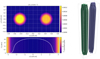 |
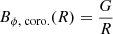
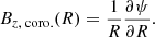
Fig. 1. Initial conditions used in the numerical simulation. Upper-left panel: map of the angular velocity at the bottom of the box. The colour scale emphasizes higher angular velocity. The uniform grid is marked. The two rotating regions have the same radius Rmax. The region on the left has a higher angular velocity (vmax.,left = 1.1 × vmax.,right). Lower-left panel: map of average plasma β as a function of z at t = 0 s. The solid curve shows the initial temperature along the z axis. Right panel: three-dimensional rendering of the initial magnetic field configuration in the box around the two flux tubes. The green field lines are twisted more quickly than the purple ones. |
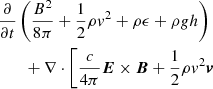
The evolution of the plasma and magnetic field in the box is described by solving the full, time-dependent MHD equations including gravity (for a curved loop), thermal conduction (including the effects of heat flux saturation), radiative losses from an optically thin plasma, and an anomalous magnetic diffusivity. The equations are solved in Eulerian, conservative form:
![$$ \begin{aligned}&\qquad \left. + \frac{\gamma }{\gamma -1} P\, \boldsymbol{v} + \boldsymbol{F}_c + \rho g h\, \boldsymbol{v} \right] = - \Lambda (T) n_e n_H + H_0, \\&P = (\gamma -1) \rho \epsilon = \frac{2 k_B}{\mu m_H} \rho T, \end{aligned} $$](/articles/aa/full_html/2023/10/aa46689-23/aa46689-23-eq5.gif)
where t is the time; ρ is the mass density; v is the plasma velocity; P is the thermal pressure; B is the magnetic field; E is the electric field; g is the gravity acceleration vector for a curved loop; I is the identity tensor; ϵ is the internal energy; j is the induced current density; η is the magnetic diffusivity;  is the electrical conductivity; T is the temperature; Fc is the thermal conductive flux; Λ(T) is the optically thin radiative losses per unit emission measure; nH and ne are the hydrogen and electron number density, respectively; mH is the hydrogen mass density; kB is the Boltzmann constant; μ = 1.265 is the mean ionic weight (relative to a proton and assuming metal abundance of solar values: X (H)≃70.7%, Y (He)≃27.4%, Z (Li − U)≃1.9%; Anders & Grevesse 1989); and H0 = 4.3 × 10⁻⁵ erg cm−3 s−1 is a volumetric heating rate that balances the initial energy losses and is used to keep the loop initially in thermal equilibrium. As shown in Eq. (5), we used the ideal gas law as an equation of state.
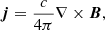
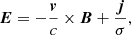
According to the induction equation (Eq. (3)), the magnetic field solenoidal condition ∇ ⋅ B = 0 formally holds at any time t, provided the initial conditions are well posed (and numerical errors are not taken into account). Ampère’s law in a non-relativistic regime (Eq. (6)) gives the current density in terms of the curl of the magnetic field. In Eq. (6), the displacement current can be neglected provided that the plasma velocity is not relativistic (i.e. v ≪ c). The electric field E is defined by Ohm’s law in Eq. (7). From this, the Poynting flux can be decomposed into three terms:
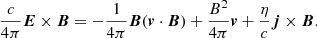
The first term on the right-hand side (- ) is significant for the driving, as it determines the energy injected in the domain by the photospheric driver. The second term (
 ) represents the flow of magnetic energy across the boundaries of the domain. Finally, the third term (
 ) is related to Ohmic dissipation and field line diffusion at the boundaries of the domain.
2.1. Thermal conduction, radiative losses, and heating
The thermal conductive flux is defined in the equations below.
![$$ \begin{aligned} \boldsymbol{F}_{\mathrm{class.} }&= - k_{\parallel } \hat{\boldsymbol{b}} ( \hat{\boldsymbol{b}} \cdot \mathbf \nabla T) - k_{\perp } \left[ \mathbf \nabla T - \hat{\boldsymbol{b}} ( \hat{\boldsymbol{b}} \cdot \mathbf \nabla T) \right], \end{aligned} $$](/articles/aa/full_html/2023/10/aa46689-23/aa46689-23-eq14.gif)
where the subscripts ∥ and ⊥ denote the components parallel and perpendicular to the magnetic field. The thermal conduction coefficients along and across the field are  and
and  , where K∥ = 9.2 × 10⁻⁷ and K⊥ = 5.4 × 10⁻¹⁶ (cgs units); ciso. is the isothermal sound speed; ϕ = 0.9 is a dimensionless free parameter;
  is a unit vector in the direction of the magnetic field; and Fsat. is the maximum flux magnitude in the direction of Fc.
The optically thin radiative losses per unit emission measure were derived from the CHIANTI v. 7.0 database (Landi & Reale 2013). We assumed coronal element abundances (Widing & Feldman 1992).
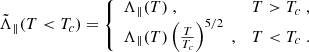
Across the transition region, the number density and the temperature change by three orders of magnitude in less than 100 km. Resolving such rapid variation and steep gradients would ordinarily require an extremely high spatial resolution and lead to unfeasible computational times (Bradshaw & Cargill 2013). The Linker–Lionello–Mikić method (Linker et al. 2001; Lionello et al. 2009; Mikić et al. 2013) allowed us artificially to broaden the transition region without significantly changing the properties of the loop in the corona, obviating that challenge. In particular, following the Linker-Lionello–Mikić approach, we modified the temperature dependence of the parallel thermal conductivity and radiative emissivity below a temperature threshold Tc = 2.5 × 10⁵ K:
According to Rosner-Tucker-Vaiana (RTV) scaling laws (Rosner et al. 1978), the volumetric heating rate H0 is sufficient to keep the corona static with an apex temperature of about 8 × 10⁵ K and a half-length of L = 2.5 × 109 cm. This provided a background atmosphere that was adopted as the initial condition, according to the hydrostatic loop model by Serio et al. (1981) and Guarrasi et al. (2014). This heating rate was not similarly scaled for temperatures below the cut-off temperature (cf. Johnston et al. 2020).
2.2. Gravity in a curved loop
We assumed that the flux tube is circularly curved only in the corona and that it is straight in the chromosphere. Thus, we considered the gravity of a curved loop in the corona:
where  is constant; G is the gravitational constant; M⊙ is the solar mass; and R⊙ is the solar radius. We note that gravitational acceleration decreases and becomes zero at the loop apex (z = 0) to account for the loop curvature. Below the corona, gravity is uniform and vertical.
2.3. The loop setup
The 3D computational domain of our reference simulation contains two flux tubes, each with a length of 5 × 109 cm and an initial temperature of approximately 106 K (see lower-left panel of Fig. 1). Their footpoints are anchored to two thick, isothermal chromospheric layers at the top and bottom of the box. As the plasma β decreases farther from the boundaries, the magnetic field expands (see Fig. 1). The initial atmosphere is the result of a preliminary simulation in which we let a domain with a vertical magnetic field relax to an equilibrium condition until the maximum velocity reached a value below 10 km s−1, as described in Guarrasi et al. (2014).
The computational box is a 3D Cartesian grid, −xM < x < xM, −yM < y < yM, and −zM < z < zM, where xM = 2yM = 8 × 108 cm, yM = 4 × 108 cm, and zM = 3.1 × 109 cm, with a staggered grid. We adopted the piecewise uniform and stretched grid sketched in Fig. 1. In particular, in the corona, we considered a non-uniform grid whose resolution degrades with height. To describe the transition region at sufficiently high resolution, the cell size there (|z|≈2.4 × 109 cm) decreases to Δr ∼ Δz ∼ 3 × 106 cm and remains constant across the chromosphere. The boundary conditions are periodic at x = ±xM and y = ±yM. Reflecting boundary conditions were set at z = ±zM. There, the magnetic field has equatorial-symmetric boundary conditions (i.e., symmetric for the normal component of the magnetic field and anti-symmetric for the tangential components).
We also performed a second numerical experiment, extending the domain in the x-direction (xM = 1.5 × 109 cm) and including a third flux tube. The results of this simulation are discussed in Sect. 5.
2.4. The plasma resistivity
We considered an anomalous plasma resistivity that is switched on only in the corona and transition region (i.e. above Tcr. = 104 K) where the magnitude of the current density exceeds a critical value, as in the following equation (e.g. Hood et al. 2009):
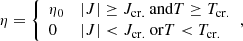
where we assumed η0 = 1014 cm−2 s−1 and Jcr. = 250 Frcm−3 s−1. The current threshold was chosen so as to avoid Ohmic heating before the onset of the avalanche process and to permit the ideal build-up to the instability. With this assumption, the minimum heating rate above the threshold is H = η0(4π|Jcr.|/c)2 ≈ 0.3 erg cm−3 s−1. Below the critical current, a minimum numerical resistivity is inevitably present, but it does not contribute any heating during the simulation.
2.5. Loop twisting
We tested the evolution of a coronal loop under the effects of a footpoint rotation. In particular, both strands were driven by coherent photospheric rotations that switch signs from one footpoint to the other. Rotation at the threads’ footpoints induces a twisting of the magnetic field lines. As flux tube torsion increases, the current density is amplified. Once the conditions for kink instability are reached, a strong current sheet forms and the critical current is exceeded, triggering magnetic diffusion and heating via Ohmic dissipation. The angular velocity ω(r) is that of a rigid body around the central axis; that is, the angular speed is constant in an inner circle and then decreases linearly in an outer annulus (Reale et al. 2016):
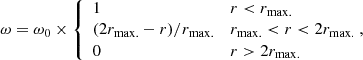
where ω0 = vmax./rmax., vmax. is the maximum tangential velocity (vϕ = ωr), and rmax. is the characteristic radius of the rotation. In this specific case, the central loop is driven at a speed that is 10% higher than the lateral ones and is equal to 1.1 km s−1. The maximum velocity achieved by twisting is always smaller than the minimum Alfvén velocity  in the domain. Moreover, the characteristic velocity (ω0 rmax.) is high enough to avoid field line slippage at the photospheric boundaries caused by numerical diffusion. The choice of a mirror-symmetric photospheric driver does not cause the further system evolution to lack generality: as the relatively high Alfvén velocities lead coronal loops to maintain a very high degree of symmetry, even when they are subjected to asymmetric photospheric motions for a long time (Cozzo et al. 2023). The rmax. parameter was set to 1200 km for both loops (see top-left panel of Fig. 1). For many recent simulations of coronal loops subject to photospheric driving, a significant challenge has been in attaining realistic driving speeds, given that there is a need to drive quickly enough to prevent slippage of field lines, which requires modelling velocities that are much faster than those observed. However, with velocities of the order of 1 km s−1, we approach typical photospheric velocity patterns (Gizon & Birch 2005; Rieutord & Rincon 2010) and benefited from growing computational resources.
2.6. Numerical computation
The calculations were performed using the PLUTO code (Mignone et al. 2007, 2012), a modular Godunov-type code for astrophysical plasmas. The code provides an algorithmic, modular multi-physics environment particularly oriented towards the treatment of astrophysical flows in the presence of discontinuities, as in the case treated here. Numerical integration of the conservation laws (Eqs. (1)–(4)) was achieved through high-resolution shock-capturing (HRSC) schemes using the finite-volume formalism where volume averages evolve in time (Mignone et al. 2007). The code is designed to make efficient use of massive parallel computers using the message passing interface library for interprocessor communications. The MHD equations were solved using the MHD module available in PLUTO, configured to compute intercell fluxes with the Harten–Lax–Van Leer approximate Riemann solver (Roe 1986), while second-order accuracy in time was achieved using a Runge-Kutta scheme. A Van Leer limiter (Sweby 1984) for the primitive variables was used. The evolution of the magnetic field was carried out adopting the constrained transport approach (Balsara & Spicer 1999) that maintains the solenoidal condition (∇ ⋅ B = 0) at machine accuracy. The PLUTO code includes optically thin radiative losses in a fractional step formalism, which preserves the second-order time accuracy, since the advection and source steps are at least second-order accurate. The radiative loss, Λ, values were taken from a look-up table. Thermal conduction was treated separately from advection terms through operator splitting. In particular, we adopted the super-time-stepping technique (Alexiades et al. 1996), which has proved to be very effective at speeding up explicit time-stepping schemes for parabolic problems. This approach is crucial when high values of plasma temperature are reached (e.g. during flares) since explicit schemes are subject to a rather restrictive stability condition (namely, Δt ≤ (Δx)2/(2α), where α is the maximum diffusion coefficient). This means the thermal conduction timescale, τcond., is shorter than the dynamical one, τdyn. (Orlando et al. 2005, 2008).
3. Basic theory
3.1. Twisting with expanding magnetic tube
Simple analytical models can predict the initial, steady-state evolution of a system provided that certain assumptions be satisfied (Hood & Priest 1979a; Browning & Hood 1989). Each loop is modelled as a cylindrically symmetric magnetic structure not interacting with the neighbouring ones. The initial magnetic field is not uniform: magnetic field lines expand from the photospheric boundaries (where B ≈ 300 G) to the upper corona (where B ≈ 10 G). As the field lines expand, the magnetic field decreases by an order of magnitude because of conservation of magnetic flux. The expansion of the field corresponds to a height that is roughly equal to the distance between the chromospheric sources, so it involves a small fraction of a coronal loop length, and thus the loop is of mostly uniform width in the corona. Field line tapering is strong in the chromosphere, where changes in the plasma beta are steeper, but weaker in the corona. In typical coronal conditions, such as high (T ≈ 1 MK) and uniform temperature, the pressure scale height is large compared with the loop length. Therefore, density and pressure can be assumed to be uniform and constant in the corona. Averaged values can be constrained from the RTV scaling laws (Rosner et al. 1978) once the total length of the loop 2L and the uniform heating rate H0 are given. At the boundaries, the photospheric driver twists the magnetic field, causing the azimuthal component to increase. Perfect line-tying to the photospheric boundaries is assumed and no field line slippage is taken into account. The driver is much slower than the Alfvén velocity so that the magnetic torsion can be assumed to be instantaneously transmitted along the whole tube.
Under these assumptions, it is possible to express the magnetic field of a single thread in cylindrical coordinates in terms of the flux function ψ as a generalized parameter:
where  . In Eq. (17), the azimuthal magnetic field component is given by a function, G, of the flux function, ψ. The function G is related to the radial profile of the twisting velocity. In the following, R denotes the radius in the corona, and r is the radius in the photosphere. Under typical coronal conditions (i.e. low plasma beta), the force-free condition,
holds. Using Eq. (17), the force-free equation is satisfied by the Grad-Shafranov equation (Grad & Rubin 1958; Shafranov 1958):
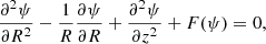
where  is a function of ψ. The third term on the left-hand side can be neglected in the corona, under the assumption of negligible field line curvature,
  (Browning & Hood 1989; Lothian & Hood 1989). As a first assumption, we considered the azimuthal velocity to be linear in z, since the twisting is equal in magnitude and opposite in direction at the two ends:

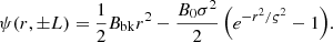
where l is a length scale that can be assumed to be equal to L, the half-length of the loop, in order that this equation matches the angular speed imposed on the boundaries. From the linearization of the ideal induction equation (Eq. (3)), with η = 0, the azimuthal component of the magnetic field in the photosphere is easily linked to the given twisting angular velocity ω(r) (see Eq. (16)):
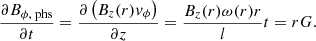
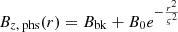
The vertical component at the photosphere, Bz, phs(r), is given by the superposition of a background magnetic field Bbk and a Gaussian function with amplitude B0 and a characteristic width ς, that is:
so that:
The magnetostatic equilibrium of a coronal loop in response to slow twisting of the photospheric footpoints can be investigated in the corona by solving the Grad–Shafranov equation:
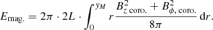
In this way, we accounted for the flux tube expansion across the chromosphere just by assuming magnetic flux conservation throughout the loop volume and force-free condition in the corona. In particular, the volume-integrated magnetic energy of a single thread in the corona is given by:
The volume-integrated kinetic energy can be roughly assessed by assuming the coronal loop to reach a steady state where the plasma is moved only by the magnetic field torsion:
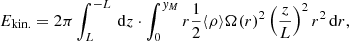
where Ω(r) is the angular velocity of the loop in the corona (the relation Ω(ψ) = ω(ψ) holds) and ⟨ρ⟩ is the averaged coronal density.
In a cylindrically symmetric flux tube, the angular velocity produces the axial current density and the azimuthal magnetic field (see Eq. (16)):
according to Eqs. (6), (16), (20), and (21). A rough but effective estimate of the maximum current density over the time is retrieved by evaluating the current density at the loop axis:
As soon as the azimuthal component of the magnetic field increases linearly with time, magnetic energy should grow quadratically and the current density should grow linearly.
3.2. Energy equations
The temporal evolution of the four energy terms (i.e. magnetic, kinetic, internal, and gravitational energy) is driven by the energy sources and sinks (background heating and radiative losses, respectively) and several energy fluxes at the boundaries of the domain (such as thermal conduction, Poynting flux, enthalpy flux, and kinetic and gravitational energy fluxes). In addition, energy transfer terms may link two different forms of energy. This is the case for Ohmic heating, which converts magnetic energy into heat, and work done per unit time by the Lorentz force, the pressure gradient, and gravity, which respectively convert kinetic energy into magnetic, thermal, and gravitational energy. The respective equations governing the evolution of magnetic, kinetic, internal, and gravitational energy are as follows:
![$$ \begin{aligned}&\qquad + \left. \frac{B^2}{4 \pi } \boldsymbol{v} + \frac{\eta }{c} \boldsymbol{j} \times \boldsymbol{B}\right] = - \frac{j^2}{\sigma } - \frac{\boldsymbol{v}}{c} \cdot \left(\boldsymbol{j} \times \boldsymbol{B} \right), \nonumber \\&\frac{\partial }{\partial t} \left(\frac{1}{2} \rho v^2 \right) + \nabla \cdot \left(\frac{1}{2} \rho v^2 \,\boldsymbol{v} \right)= - \boldsymbol{v} \cdot \nabla P + \frac{\boldsymbol{v}}{c} \left( \boldsymbol{j} \times \boldsymbol{B} \right) \\&\qquad \qquad \qquad \qquad \qquad \qquad + \rho \, \boldsymbol{v} \cdot \boldsymbol{g}, \nonumber \end{aligned} $$](/articles/aa/full_html/2023/10/aa46689-23/aa46689-23-eq43.gif)
![$$ \begin{aligned} \frac{\partial (\rho \epsilon )}{\partial t} + \nabla \cdot \left[ \frac{\gamma }{\gamma -1} P \,\boldsymbol{v} + \nabla \cdot \boldsymbol{F}_c \right]&= \boldsymbol{v} \cdot \nabla P - \Lambda (T) n_e n_H \end{aligned} $$](/articles/aa/full_html/2023/10/aa46689-23/aa46689-23-eq44.gif)
The sum of the four equations gives the energy equation (Eq. (4)) discussed in Sect. 2. Terms on the left-hand sides include rates of change in energy (the derivatives with respect to time) and energy fluxes (i.e. surface terms, which appear here as divergences). Energy transfer terms, sources, and sinks are on the right-hand sides.
4. Results
4.1. Continued driving: Evolution before the instability
The box size is 6.2 Mm in the z direction. The chromosphere extends for 0.7 Mm on both sides, and the corona (including the transition region) is in the middle 2L = 5 × 109 cm (see Sect. 2.1). In the following, we cautiously restricted our analysis to the inner domain between z = ±2 × 109 cm in order to avoid any possible undesired contributions from expected changes in transition region height. Since boundary conditions are periodic at the side boundaries of the box, fluxes were only evaluated at the upper and lower boundaries of the sub-domain (i.e. at z = ±2 × 109 cm).
Initially, the two flux tubes were slowly twisted at a speed much slower than the Alfvén speed. As a consequence, the initial evolution of the magnetic structure is through quasi-steady states. In particular, an azimuthal magnetic field component grows almost linearly with time. The magnetic torsion is transmitted to the coronal part of the magnetic tube (i.e. at |z|< 2 × 109 cm) after two hundred seconds, in accordance with the time estimated for a magnetic signal to cross the chromospheric layer.
Figure 2 shows the rate of change of the total energy, which is given as the sum of magnetic, kinetic, thermal, and gravitational energy. The total energy is not constant inside the coronal volume as a result of incoming fluxes at the chromospheric boundaries of the domain (such as Poynting flux, kinetic energy flux, enthalpy flux, gravitational energy flux, and thermal conduction), energy sources (background heating), and sinks (radiative losses). The total energy in the system, accounting for incoming and outgoing fluxes (see Eq. (4)), is approximately conserved throughout the numerical experiment. Amongst all the external contributions, the Poynting flux is dominant during the build-up of the twisting.
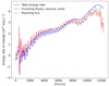 |
Fig. 2. Evolution of the rate of change of the total energy, incoming fluxes, sources, and sinks for the reference simulation. The blue curve indicates the change in total energy over time, given by the sum of internal, kinetic, magnetic, and gravitational energies of the system, plotted as functions of time, before the onset of the instability. The red curve represents the sum of the total fluxes, energy sources, and sinks as a function of time before the onset of the instability. The closeness of the blue and red curves demonstrates the approximate energy conservation in the domain. The dashed black curve depicts the Poynting flux, which is the dominant flux and adds to the magnetic energy. |
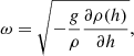
The initial evolution of the system might be seen as the superposition of a long-lasting and steady tube twisting (where magnetic energy and current density slowly grow as a consequence of the field line torsion) and a wave-like response to the induced dynamics (where oscillations of short characteristic timescales are damped with time). In particular, long-period oscillation (P ≈ 360 s) is clearly visible in Fig. 2 and in Fig. 3, the latter of which shows the work done by the pressure gradient and the work done by gravity as functions of time. Those features might be associated with Brunt–Väisälä oscillations whose characteristic frequency is
 |
Fig. 3. Fourier transform of pressure work, gravity work, and kinetic energy rates. The blue curve indicates the Fourier transform of the work done by pressure gradients per unit time, before the onset of the instability. The red curve represents the Fourier transform of the work done by gravity force per unit time, before the onset of the instability. Both curves show a peak around T ≈ 365 s (identified by eye). The green curve depicts the Fourier transform of the kinetic energy before the onset of the instability. It shows a peak around 180 s. |
where  gives the height in a semi-circular loop. In particular, a frequency of 2.76 × 10⁻³ s−1 (corresponding to a period of approximately 360 s) matches the theoretical value at transition region heights, suggesting that the nature of this oscillation might be associated with buoyancy movements in the upper chormospheric layers. Alfvén waves appear in each thread as azimuthal modes with a period of nearly 50 s.
In Fig. 4, the kinetic energy reaches a steady state value around a time of 6000 s and remains there until about t = 11 000 s, when it exponentially increases as the first kink instability occurs. The theoretical limit, computed from Eq. (27) and shown as a red dashed line, agrees with the actual volume-averaged kinetic energy. The oscillations in kinetic energy have a period of approximately t = 180 s (see Fig. 3) and are the result of magnetosonic waves. Moreover, the growth of the kinetic energy during the onset of the ideal kink instability is, as expected, exponential with time. This is shown in the internal panel of Fig. 4. In particular, the slope of the exponential increase matches with the theoretical value τ = 0.1 × 2L/vA, where vA is the Alfvén velocity (Van der Linden & Hood 1999; Hood et al. 2009).
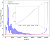 |
Fig. 4. Kinetic energy damping before the instability onset. In blue is the total kinetic energy, plotted as a function of time, in the time leading up to the instability. The last exponential rise shows the time at which the first thread is disrupted. In dashed red is a theoretical estimation of the steady state based on the model described in Eq. (27). As waves are progressively damped, the total kinetic energy is expected to tend towards this theoretical steady state prior to the instability. |
Figure 5 shows that the magnetic energy determined from the simulation is very close to the prediction of the theoretical model presented in the previous section. The quadratic increase of the magnetic energy is determined by the linear growth of the azimuthal component of the magnetic field during the twisting.
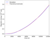 |
Fig. 5. Evolution of the volume integrated magnetic energy prior to the instability. In blue is the total magnetic energy before the onset of the instability, plotted as a function of time. In dashed red is a theoretical estimate based on the model described in Sect. 3, which grows through the energy input by photospheric driving. |
The vertical component of the current density dominates over the other ones. It also grows linearly in time as a consequence of the magnetic tube twisting (see Fig. 6). As assumed in Eq. (29), the maximum current intensity is along the axis of each flux tube As shown in Fig. 7, the axial current remains positive around the centres of the strands. On the outer edge, there is a neutralizing negative current, ensuring the net axial current remains zero.
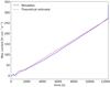 |
Fig. 6. Evolution of the maximum current density. The solid, blue curve represents the maximum current intensity, before the onset of the instability, as a function of time. In dashed red is the theoretical estimate based on the model described in Sect. 3. |
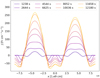 |
Fig. 7. Profiles of the apex current intensity along the x-axis (y = 0) at different times. |
4.2. Onset of the instability
The first tube becomes unstable after around 12 400 s. We estimated the amount of twist, defined as Φ = 2πN (with N the number of twists in the unstable strand), at the time of the kink instability. We considered both the maximum tangential photospheric velocity vϕ and an averaged value 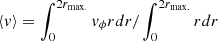 . In the first case, the Φ ≈ 10, while in the second one it is smaller by a factor of two. In both cases, Φ is of the same order of magnitude as previous results, such as the Kruskal-Shafranov condition (ΦKS = 3.3 π; Priest 2014).
The onset of the first kink instability and the subsequent MHD cascade can be followed by inspecting the current density and velocity evolution. For instance, Fig. 8 shows the current density distribution (first column) and the velocity field (second column) over the loop mid-plane at four different times. In the first panel (t = 12 400 s), the onset of the first kink instability is shown: the unstable flux tube begins to flex owing to the growing magnetic pressure imbalance. Consequently, a single current sheet forms at the edge of the loop, and the velocity grows at its sides. Then, in the second panel (t = 12 500 s), the current sheet fragments in a turbulent way (see the velocity map) into smaller current sheets, and the entire structure expands to interact with the neighbouring loop. This causes the second strand’s instability. The third (t = 12 550 s) and fourth (t = 12 600 s) panels show the evolution of the MHD cascade (i.e. second loop disruption) triggered by the first kink instability. Throughout the process, zones of high plasma velocity on the horizontal mid-plane spread over regions of high current density. This is expected since plasma is mostly accelerated by magnetic forces where magnetic field gradients are higher.
 |
Fig. 8. Onset and evolution of the MHD avalanche. First column: horizontal cut of the current density across the mid-plane at times (from the top) t = 12 400 s (onset of first kink instability), t = 12 500 s, t = 12 550 s (second strand’s disruption), and t = 12 600 s. Second column: horizontal cut of the velocity across the mid-plane at the same four times. The arrows show the orientation of the velocity field. The colour maps evaluate the intensity of the vertical component of the velocity field. Third column: terminal locations (z = L) of the sample field lines at the same four times. The red field lines (spots) depart from the z = −L footpoint on the left (red shaded region), and the blue field lines depart from the right (blue shaded region). Initially, the red and blue field lines are randomly distributed inside the blue and red circles, respectively. Subsequent starting locations at the lower boundary points were determined at later times by tracking their locations in response to the photospheric motions. |
The average temperature peaks 100 seconds after the onset of the avalanche process, while the average density and radiative losses reach the maximum value after a further period of 800 s (see first panel of Fig. 9). The turbulent evolution of the system is difficult to follow, but quantitative information on its dynamics can be obtained from the maximum current, temperature, and velocity evolution shown in Fig. 9. The three plots show the same qualitative behaviour with some high peaks around t = 12 500 s; that is, during large heating events corresponding to dissipation of relatively large current sheets. In particular, the first group of peaks occurs during the onset of the first kink instability. The second and third groups correspond to the times when the second loop is destabilized and when it is finally disrupted, respectively. Another peak in the current intensity occurs at t = 13 000 s and is followed by a moderate enhancement in the loop temperature and velocity. It is produced by the formation and subsequent dissipation of a big current sheet induced by the continuous driving at the boundaries.
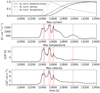 |
Fig. 9. Global evolution of the MHD avalanche. From top to bottom: average normalized radiative losses, density and temperature in the corona, maximum current density, maximum temperature, and maximum velocity against time. The red vertical lines mark the times of large heating events. |
The dissipation of the multi-threaded loop into smaller current sheets can be traced by following the magnetic field lines connectivity over time. The third column of Fig. 8 shows the end points of some field lines on the upper boundary plane z = zmax.. Red dots correspond to field lines connected at the bottom to the left footpoint (i.e. z = −zmax.). Conversely, blue dots refer to field lines connected at the bottom to the footpoint on the right. Field lines were traced from the bottom side of the box and mapped into the upper one using a second-order Runge-Kutta integration scheme. The location of the starting points at z = −zmax. were updated according to the imposed rotation, while the points at the opposite side were expected to change as the field lines move or change by reconnection. It is easy to see that the field line connectivity changes as soon as the MHD cascade takes place and that magnetic reconnection has occurred in the meantime. Indeed, during the avalanche process, field lines from each strand become entangled and eventually cross the lateral boundaries of the domain. The same thing is likewise evident in Fig. 10, where field lines in the box are shown in full-3D rendering. The field lines were computed using a fourth order Runge-Kutta scheme, and colour was attributed depending on where on the photosphere the starting points were placed. As the twisting triggers the kink instability, field lines reconnect with each other. At the end of the process, some light blue and purple lines connect different loop footpoints.
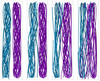 |
Fig. 10. Three-dimensional rendering of the magnetic field lines in the box around the two flux tubes at different times. Far left panel: field lines at t = 12 400 s (onset of first kink instability). Middle left panel: field lines at t = 12 500 s. Middle right panel: field lines at t = 12 550 s (second loop disruption). Far right panel: field lines at t = 12 600 s. The change in the field line connectivity during the evolution of the MHD cascade is highlighted by the different colours. |
The energetics of the numerical experiment reflect the physical processes that drive the system dynamics. Figure 11 shows the evolution of the four energy components (i.e. magnetic, kinetic, thermal, and gravitational energy). The magnetic energy dominates over the other components during the initial, smooth evolution of the system. As mentioned above, the main source of energy derives from the Poynting flux (see Fig. 2). The net effect of thermal conduction, radiative losses, and background heating is negligible provided that the magnetic field changes are slow compared with the radiative and conductive timescales. In Fig. 12, the sum of the time-integrated thermal flux, radiative losses, and uniform heating is practically zero, while the thermal conduction dominates over the radiative losses, as expected in typical coronal conditions.
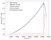 |
Fig. 11. Magnetic (purple), internal (pink), kinetic (orange), and gravitational (yellow) energies as functions of time. The black is the total energy given as the sum of the four energy terms. The onset of the avalanche is marked with a vertical red dashed line. |
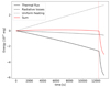 |
Fig. 12. Time-integrated thermal flux (solid black), radiative losses (dashed black), and background heating (dotted black) as functions of time. The solid red curve is the sum of the three contributions. The onset of the avalanche is marked with a vertical red dashed line. |
After the onset of the MHD avalanche, the magnetic energy rapidly drops. The kinetic energy increases exponentially but remains at least one order of magnitude smaller than the magnetic energy. Most of the magnetic energy gained, through footpoint driving, is converted into heat, and the steep rise in thermal energy follows the plasma acceleration. Figure 13 shows how the rate of change in magnetic energy matches the instantaneous Ohmic heating and how it, in turn, influences the rate of change in heating.
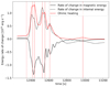 |
Fig. 13. Rates of change in magnetic (solid black) and internal (dashed black) energies and Ohmic heating (red) as functions of time. The vertical red solid lines highlight times of large heating events. The onset of the avalanche is marked with a vertical red dashed line. |
Several heat pulses released after the multiple magnetic reconnection events enhance the thermal conductive flux towards both transition regions (see Fig. 12). The heat flow was then slowed down in the chromosphere because conduction is less efficient at cooler temperatures. As a consequence, an excess of pressure accumulates in the transition region and the top of the chromosphere. This creates the pressure gradient that causes the evaporative upflow. The plasma expanding upwards, in turn, leads to an increase in the coronal density inside the magnetic structure. The sudden growth of the gravitational potential energy traces this strong mass flow upwards, as shown in Fig. 14. After the beginning of the MHD avalanche, the gravitational energy increases as a consequence of the chromospheric plasma evaporation in the coronal volume. It supplied gravitational energy flux at the boundaries while the remaining contribution to the potential energy is given by the work done by the gravity force to distribute this denser plasma over the entire loop length.
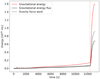 |
Fig. 14. Gravitational energy (red), time-integrated gravitational energy flux (solid black), and work done by gravity (dashed black) as functions of time. The onset of the avalanche is marked with a vertical red dashed red line. |
Figure 15 shows the average vertical thermal flux, radiative losses, density, and temperature as a function of time and height. The strongest thermal flux (first panel) developed at the times when each loop is disrupted (i.e. when the temperature gradient is greatest). The heat flux propagates towards the upper and lower transition regions and was stronger in the corona. In contrast, the radiative losses (second panel) were stronger at later times, when the density (third panel) has increased by chromospheric evaporation. The biggest contribution is localized in the transition region where the rates exceed the coronal radiative losses by at least two orders of magnitude. As heating released during the MHD avalanche rapidly spread (in few tens of seconds) along the tube, temperature (fourth panel) rises uniformly. It then slowly decreases from 10 MK to 1 MK on a timescale of 1000 s.
 |
Fig. 15. Average vertical thermal flux, radiative losses, plasma density, and temperature against time (on the horizontal axis) and height (z; on the vertical axis). The averaging is on the horizontal planes. The region of the domain where the temperature exceeds 104 K (i.e. transition region and corona) is bounded (magenta lines). |
4.3. Three-stranded loop simulation
The propagation of the instability described so far is an avalanche process that can extend to increasing numbers of nearby flux tubes (Hood et al. 2016). To ensure this progression, we performed a second numerical experiment with three interacting strands within a coronal loop. The initial configuration of the magnetic structure is shown in the left panel of Fig. 16. As in the previous case, this magnetic structure is embedded in a stratified atmosphere with a cold (T ≃ 104 K) chromospheric layer and a hot and tenuous corona (T ≃ 106 K and n ≃ 109 cm−3). Equations (1)–(7) summarize the underlying physics driving the evolution of the system, as discussed in Sect. 2. As in the first case, one of the magnetic strands is twisted at its footpoint faster than the others and becomes kink unstable. The right panel of Fig. 16 shows the propagation of the instability from a central, faster tube to the two adjacent tubes. As expected, the first unstable strand triggers the global dissipation of the magnetic structure into smaller current sheets. Heating by Ohmic dissipation is localized inside relatively small regions where the current density is higher. These current sheets develop and spread in a turbulent way throughout the entire extension of the domain.
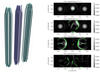 |
Fig. 16. Three-threaded coronal loop simulation: initial condition and evolution of the MHD avalanche. Left panel: three-dimensional rendering of the initial magnetic field configuration in the proximity of each coronal loop (for the second model, with three strands). The purple field lines were subjected to a faster twisting driver than the green ones. Right panel: horizontal cut of the Ohmic heating per unit time and per unit volume at the middle of the box at different times. From the top down, these times are: t = 11 200 s (onset of first kink instability), t = 11 400 s, t = 11 800 s (disruption of the second and third strands), and t = 11 900 s. The green filaments indicate areas where the current density exceedes the threshold value for dissipation. |
5. Discussion and conclusions
This work addresses the energy released impulsively in the corona under strong magnetic stresses. In particular, we have shown that MHD avalanches are efficient mechanisms for fast release of magnetic energy in the solar corona progressively stored by slow, uniform photospheric motions. We describe a system consisting of two neighbouring twisted flux tubes. These interacting flux tubes comprise a stratified atmosphere including chromospheric layers, a thin transition region to the corona, and an associated transition from high-β to low-β regions. Our model includes the effects of thermal conduction and of optically thin radiation. Rotation of the plasma at the upper and lower boundaries of our computational domain applies twisting to the magnetic flux tubes. Since line-tying of the field lines at the photospheric boundaries is expected to be maintained over time by high plasma beta values and a sufficient spatial resolution, each loop can develop high levels of twist, as the azimuthal component of the magnetic field increases. Above a certain stress threshold, the structure becomes kink-unstable and suddenly relaxes to a new equilibrium configuration (Hood et al. 2009). In particular, since one strand is twisted faster than the other, that strand will become unstable before the other and trigger the avalanche process that will, in turn, spread as it affects the neighbouring flux tube. Magnetic reconnection between unstable flux tubes causes bursty and diffuse energy release (similar to a nanoflare storm) and changes the field connectivity. Moreover, through repeated reconnection events, the system relaxes towards the minimum energy state. The system undergoes an initial dynamic phase where the plasma is rapidly accelerated. The initial helical current sheet progressively fragments in a turbulent way into smaller current sheets, which, in turn, dissipate magnetic energy via Ohmic heating. As soon as the steep rise in kinetic energy is damped in the corona, the released heating rapidly increases the coronal temperatures and, consequently, the pressure scale-height. As a consequence of that process, the steep rise in temperature is followed by a progressive coronal density enhancement due to chromospheric evaporation.
Results achieved in this paper agree with those found by Hood et al. (2009;, 2016), and Reid et al. (2018), but also go further and extend them. In particular, we demonstrate that even inside a stratified atmosphere, highly twisted loops with zero net current undergo the non-linear phase of the kink instability where reconnection in a single current sheet triggers the fragmentation of the flux tubes at multiple reconnection sites. In particular, once the first unstable strand is disrupted, it coalesces with the neighbouring strands, inducing an MHD cascade, as found in uniform coronal atmospheres (Tam et al. 2015; Hood et al. 2016; Reid et al. 2018).
As shown in Fig. 13, magnetic energy is released in discrete bursts as stable strands are disrupted and single current sheets are dissipated. This bursty heating does not show evidence of reaching a steady state.
Thermal conduction is very effective in spreading heating along field lines, and this leads to the filamentary structuring in loop temperature. Also, as shown in Fig. 9, because of thermal conduction, the temperature grows to about 107 K, which is much cooler than the temperatures of approximately 108 K found in Hood et al. (2009). Peak temperatures of a few tens of millions of kelvin as well as variations in magnetic and internal energy of 1027 erg are found in our simulations. They agree with those measured from microflare observations (Testa & Reale 2020).
Radiation also has an important effect on the temperature distribution. Radiative losses are stronger across the transition region, where the plasma density is higher. As the upper atmosphere is heated, this layer acts as a thermostat for the corona since it tends to restore the initial coronal temperature. Indeed, it maintains the temperature gradient that allows heat to flow out of the corona.
A deep chromospheric layer is important to guarantee line-tying throughout the whole evolution of the coronal loop. With this layer in place, photospheric motions can slowly twist the magnetic flux tubes expanding across the chromospheric layer. At the same time, the chromosphere acts as a reservoir of dense plasma that can flow into the corona as a consequence of impulsive heating. Modelling the chromospheric evaporation and the resulting increase of the loop emissivity is fundamental to corroborate the results through comparison with EUV and X-ray observations of dynamic coronal loops.
As shown in Sect. 4.3, the propagation of the instability is an avalanche process that can extend to increasing numbers of nearby flux tubes (Hood et al. 2016). In conclusion, this work confirms, and constrains the conditions for, the propagation of a kink instability amongst a cluster of flux tubes, including a more complete, stratified loop atmosphere, as well as important physical effects, in particular thermal conduction and optically thin radiative losses. The avalanche can trigger the ignition and heating of a large-scale coronal loop with parameters not far from those inferred from the observations.
The reconfiguration of the magnetic structure and the resulting plasma dynamics have been found to occur at timescales on the order of 10 s and over spatial scales smaller than one arcsecond. The detection of these small scales involved in coronal heating release will be the target of high-resolution spectroscopic observations of future missions, such as MUSE (Cheung et al. 2022; De Pontieu et al. 2022) and SOLAR-C/EUVST (Shimizu et al. 2020). Additionally, specific diagnostics will be the subject of a forthcoming investigation.
Acknowledgments
G.C., P.P. and F.R. acknowledge support from ASI/INAF agreement n. 2022-29-HH.0 and from italian Ministero dell’Universitá e della Ricerca (MUR). J.R., A.W.H. and G.C. gratefully acknowledge the financial support of the Science and Technology Facilities Council (STFC) through Consolidated Grants ST/S000402/1 and ST/W001195/1 to the University of St Andrews. This work made use of the HPC system MEUSA, part of the Sistema Computazionale per l’Astrofisica Numerica (SCAN) of INAF-Osservatorio Astronomico di Palermo.
References
- Alexiades, V., Amiez, G., & Gremaud, P.-A. 1996, Commun. Numer. Methods Eng., 12, 31 [Google Scholar]
- Anders, E., & Grevesse, N. 1989, Geochim. Cosmochim. Acta, 53, 197 [Google Scholar]
- Antolin, P., Pagano, P., Testa, P., Petralia, A., & Reale, F. 2021, Nat. Astron., 5, 54 [NASA ADS] [CrossRef] [Google Scholar]
- Balsara, D. S., & Spicer, D. S. 1999, J. Comput. Phys., 149, 270 [NASA ADS] [CrossRef] [Google Scholar]
- Baty, H., & Heyvaerts, J. 1996, A&A, 308, 935 [NASA ADS] [Google Scholar]
- Berghmans, D., Auchère, F., Long, D. M., et al. 2021, A&A, 656, L4 [NASA ADS] [CrossRef] [EDP Sciences] [Google Scholar]
- Botha, G. J. J., Arber, T. D., & Hood, A. W. 2011, A&A, 525, A96 [NASA ADS] [CrossRef] [EDP Sciences] [Google Scholar]
- Bradshaw, S. J., & Cargill, P. J. 2013, ApJ, 770, 12 [NASA ADS] [CrossRef] [Google Scholar]
- Brooks, D. H., Warren, H. P., & Landi, E. 2021, ApJ, 915, L24 [NASA ADS] [CrossRef] [Google Scholar]
- Browning, P. 2003, A&A, 400, 355 [NASA ADS] [CrossRef] [EDP Sciences] [Google Scholar]
- Browning, P., & Hood, A. 1989, Sol. Phys., 124, 271 [NASA ADS] [CrossRef] [Google Scholar]
- Browning, P., & Priest, E. 1986, A&A, 159, 129 [NASA ADS] [Google Scholar]
- Browning, P., Gerrard, C., Hood, A., Kevis, R., & Van der Linden, R. 2008, A&A, 485, 837 [NASA ADS] [CrossRef] [EDP Sciences] [Google Scholar]
- Chen, Y., Przybylski, D., Peter, H., et al. 2021, A&A, 656, L7 [NASA ADS] [CrossRef] [EDP Sciences] [Google Scholar]
- Cheung, M. C., Martínez-Sykora, J., Testa, P., et al. 2022, ApJ, 926, 53 [NASA ADS] [CrossRef] [Google Scholar]
- Cozzo, G., Pagano, P., Petralia, A., & Reale, F. 2023, Symmetry, 15, 627 [NASA ADS] [CrossRef] [Google Scholar]
- Del Zanna, L., Landi, S., Papini, E., Pucci, F., & Velli, M. 2016, J. Phys. Conf. Ser., 719 [Google Scholar]
- De Pontieu, B., Testa, P., Martínez-Sykora, J., et al. 2022, ApJ, 926, 52 [NASA ADS] [CrossRef] [Google Scholar]
- Gabriel, A. 1976, Philos. Trans. Royal Soc. London Ser. A Math. Phys. Sci., 339 [Google Scholar]
- Gizon, L., & Birch, A. C. 2005, Liv. Rev. Solar Phys., 2, 6 [Google Scholar]
- Gomez, D. O., Martens, P. C., & Golub, L. 1993, ApJ, 405, 767 [NASA ADS] [CrossRef] [Google Scholar]
- Grad, H., & Rubin, H. 1958, in Proceedings of the Second United Nations International Conference on the Peaceful Uses of Atomic Energy, 31, 190 [Google Scholar]
- Guarrasi, M., Reale, F., Orlando, S., Mignone, A., & Klimchuk, J. 2014, A&A, 564, A48 [NASA ADS] [CrossRef] [EDP Sciences] [Google Scholar]
- Heyvaerts, J., & Priest, E. R. 1983, A&A, 117, 220 [NASA ADS] [Google Scholar]
- Hood, A., & Priest, E. 1979a, A&A, 77, 233 [NASA ADS] [Google Scholar]
- Hood, A. W., & Priest, E. 1979b, Sol. Phys., 64, 303 [NASA ADS] [CrossRef] [Google Scholar]
- Hood, A. W., Browning, P., & Van der Linden, R. 2009, A&A, 506, 913 [NASA ADS] [CrossRef] [EDP Sciences] [Google Scholar]
- Hood, A. W., Cargill, P., Browning, P., & Tam, K. 2016, ApJ, 817, 5 [NASA ADS] [CrossRef] [Google Scholar]
- Ishikawa, R., Bueno, J. T., del Pino Alemán, T., et al. 2021, Sci. Adv., 7, 8406 [NASA ADS] [CrossRef] [Google Scholar]
- Johnston, C. D., Cargill, P. J., Hood, A. W., et al. 2020, A&A, 635, A168 [NASA ADS] [CrossRef] [EDP Sciences] [Google Scholar]
- Klimchuk, J. A. 2006, Sol. Phys., 234, 41 [Google Scholar]
- Klimchuk, J. A. 2009, ASP Conf. Ser., 415, 221 [NASA ADS] [Google Scholar]
- Klimchuk, J. A. 2015, Philos. Trans. Royal Soc. A Math. Phys. Eng. Sci., 373, 20140256 [NASA ADS] [Google Scholar]
- Landi, E., & Reale, F. 2013, ApJ, 772, 71 [NASA ADS] [CrossRef] [Google Scholar]
- Linker, J. A., Lionello, R., Mikić, Z., & Amari, T. 2001, J. Geophys. Res., 106, 25165 [NASA ADS] [CrossRef] [Google Scholar]
- Lionello, R., Linker, J. A., & Mikić, Z. 2009, ApJ, 690, 902 [CrossRef] [Google Scholar]
- Long, D. M., Valori, G., Pérez-Suárez, D., Morton, R. J., & Vásquez, A. M. 2017, A&A, 603, A101 [NASA ADS] [CrossRef] [EDP Sciences] [Google Scholar]
- Lothian, R., & Hood, A. 1989, Sol. Phys., 122, 227 [NASA ADS] [CrossRef] [Google Scholar]
- Mignone, A., Bodo, G., Massaglia, S., et al. 2007, ApJS, 170, 228 [Google Scholar]
- Mignone, A., Flock, M., Stute, M., Kolb, S., & Muscianisi, G. 2012, A&A, 545, A152 [NASA ADS] [CrossRef] [EDP Sciences] [Google Scholar]
- Mikić, Z., Schnack, D. D., & Van Hoven, G. 1990, ApJ, 361, 690 [CrossRef] [Google Scholar]
- Mikić, Z., Lionello, R., Mok, Y., Linker, J. A., & Winebarger, A. R. 2013, ApJ, 773, 94 [Google Scholar]
- Mondal, S. 2021, Sol. Phys., 296, 131 [NASA ADS] [CrossRef] [Google Scholar]
- Müller, D., Cyr, O. S., Zouganelis, I., et al. 2020, A&A, 642, A1 [NASA ADS] [CrossRef] [EDP Sciences] [Google Scholar]
- Orlando, S., Peres, G., Reale, F., et al. 2005, A&A, 444, 505 [NASA ADS] [CrossRef] [EDP Sciences] [Google Scholar]
- Orlando, S., Bocchino, F., Reale, F., Peres, G., & Pagano, P. 2008, ApJ, 678, 274 [NASA ADS] [CrossRef] [Google Scholar]
- Parker, E. 1972, ApJ, 174, 499 [NASA ADS] [CrossRef] [Google Scholar]
- Parker, E. N. 1988, ApJ, 330, 474 [Google Scholar]
- Parnell, C. E., & De Moortel, I. 2012, Philos. Trans. Royal Soc. A Math. Phys. Eng. Sci., 370, 3217 [NASA ADS] [Google Scholar]
- Priest, E. 2014, Magnetohydrodynamics of the Sun (Cambridge University Press) [Google Scholar]
- Reale, F. 2014, Liv. Rev. Sol. Phys., 11, 1 [NASA ADS] [Google Scholar]
- Reale, F., Orlando, S., Guarrasi, M., et al. 2016, ApJ, 830, 21 [CrossRef] [Google Scholar]
- Reid, J., Hood, A. W., Parnell, C. E., Browning, P., & Cargill, P. 2018, A&A, 615, A84 [NASA ADS] [CrossRef] [EDP Sciences] [Google Scholar]
- Reid, J., Cargill, P., Hood, A. W., Parnell, C. E., & Arber, T. D. 2020, A&A, 633, A158 [NASA ADS] [CrossRef] [EDP Sciences] [Google Scholar]
- Rieutord, M., & Rincon, F. 2010, Liv. Rev. Sol. Phys., 7, 1 [NASA ADS] [Google Scholar]
- Rochus, P., Auchère, F., & Berghmans, D., et al. 2020, A&A, 642, A8 [NASA ADS] [CrossRef] [EDP Sciences] [Google Scholar]
- Roe, P. L. 1986, Annu. Rev. Fluid Mech., 18, 337 [NASA ADS] [CrossRef] [Google Scholar]
- Rosner, R., Tucker, W. H., & Vaiana, G. 1978, ApJ, 220, 643 [NASA ADS] [CrossRef] [Google Scholar]
- Serio, S., Peres, G., Vaiana, G., Golub, L., & Rosner, R. 1981, ApJ, 243, 288 [NASA ADS] [CrossRef] [Google Scholar]
- Shafranov, V. D. 1958, Sov. Phys. J. Exp. Theor. Phys., 6, 545 [NASA ADS] [Google Scholar]
- Shimizu, T., Imada, S., Kawate, T., et al. 2020, SPIE, 11444, 113 [Google Scholar]
- Solanki, S. K., del Toro Iniesta, J. C., Woch, J., et al. 2020, A&A, 642, A11 [NASA ADS] [CrossRef] [EDP Sciences] [Google Scholar]
- SPICE Consortium, (Anderson, M., et al.) 2020, A&A, 642, A14 [NASA ADS] [CrossRef] [EDP Sciences] [Google Scholar]
- Sweby, P. K. 1984, SIAM journal on numerical analysis, 21, 995 [CrossRef] [Google Scholar]
- Tam, K. V., Hood, A. W., Browning, P., & Cargill, P. 2015, A&A, 580, A122 [NASA ADS] [CrossRef] [EDP Sciences] [Google Scholar]
- Taylor, J. B. 1974, Phys. Rev. Lett., 33, 1139 [Google Scholar]
- Taylor, J. 1986, Rev. Mod. Phys., 58, 741 [Google Scholar]
- Testa, P., & Reale, F. 2020, ApJ, 902, 31 [NASA ADS] [CrossRef] [Google Scholar]
- Vadawale, S. V., Mithun, N., Mondal, B., et al. 2021, ApJ, 912, L13 [NASA ADS] [CrossRef] [Google Scholar]
- Vaiana, G., Krieger, A., & Timothy, A. 1973, Sol. Phys., 32, 81 [NASA ADS] [CrossRef] [Google Scholar]
- Van der Linden, R., & Hood, A. 1999, A&A, 346, 303 [Google Scholar]
- Vesecky, J., Antiochos, S., & Underwood, J. 1979, ApJ, 233, 987 [NASA ADS] [CrossRef] [Google Scholar]
- Viall, N. M., & Klimchuk, J. A. 2011, ApJ, 738, 24 [Google Scholar]
- Widing, K., & Feldman, U. 1992, ApJ, 392, 715 [NASA ADS] [CrossRef] [Google Scholar]
- Woltjer, L. 1958, Proc. Natl. Acad. Sci., 44, 489 [NASA ADS] [CrossRef] [Google Scholar]
- Yang, Z., Bethge, C., Tian, H., et al. 2020, Science, 369, 694 [Google Scholar]
- Yeates, A. R., Hornig, G., & Wilmot-Smith, A. L. 2010, Phys. Rev. Lett., 105, 085002 [NASA ADS] [CrossRef] [Google Scholar]
- Zhukov, A. N., Mierla, M., Auchère, F., et al. 2021, A&A, 656, A35 [NASA ADS] [CrossRef] [EDP Sciences] [Google Scholar]
- Zirker, J. B. 1993, Sol. Phys., 148, 43 [NASA ADS] [CrossRef] [Google Scholar]
All Figures
|
Fig. 1. Initial conditions used in the numerical simulation. Upper-left panel: map of the angular velocity at the bottom of the box. The colour scale emphasizes higher angular velocity. The uniform grid is marked. The two rotating regions have the same radius Rmax. The region on the left has a higher angular velocity (vmax.,left = 1.1 × vmax.,right). Lower-left panel: map of average plasma β as a function of z at t = 0 s. The solid curve shows the initial temperature along the z axis. Right panel: three-dimensional rendering of the initial magnetic field configuration in the box around the two flux tubes. The green field lines are twisted more quickly than the purple ones. |
| In the text | |
|
Fig. 2. Evolution of the rate of change of the total energy, incoming fluxes, sources, and sinks for the reference simulation. The blue curve indicates the change in total energy over time, given by the sum of internal, kinetic, magnetic, and gravitational energies of the system, plotted as functions of time, before the onset of the instability. The red curve represents the sum of the total fluxes, energy sources, and sinks as a function of time before the onset of the instability. The closeness of the blue and red curves demonstrates the approximate energy conservation in the domain. The dashed black curve depicts the Poynting flux, which is the dominant flux and adds to the magnetic energy. |
| In the text | |
|
Fig. 3. Fourier transform of pressure work, gravity work, and kinetic energy rates. The blue curve indicates the Fourier transform of the work done by pressure gradients per unit time, before the onset of the instability. The red curve represents the Fourier transform of the work done by gravity force per unit time, before the onset of the instability. Both curves show a peak around T ≈ 365 s (identified by eye). The green curve depicts the Fourier transform of the kinetic energy before the onset of the instability. It shows a peak around 180 s. |
| In the text | |
|
Fig. 4. Kinetic energy damping before the instability onset. In blue is the total kinetic energy, plotted as a function of time, in the time leading up to the instability. The last exponential rise shows the time at which the first thread is disrupted. In dashed red is a theoretical estimation of the steady state based on the model described in Eq. (27). As waves are progressively damped, the total kinetic energy is expected to tend towards this theoretical steady state prior to the instability. |
| In the text | |
|
Fig. 5. Evolution of the volume integrated magnetic energy prior to the instability. In blue is the total magnetic energy before the onset of the instability, plotted as a function of time. In dashed red is a theoretical estimate based on the model described in Sect. 3, which grows through the energy input by photospheric driving. |
| In the text | |
|
Fig. 6. Evolution of the maximum current density. The solid, blue curve represents the maximum current intensity, before the onset of the instability, as a function of time. In dashed red is the theoretical estimate based on the model described in Sect. 3. |
| In the text | |
|
Fig. 7. Profiles of the apex current intensity along the x-axis (y = 0) at different times. |
| In the text | |
|
Fig. 8. Onset and evolution of the MHD avalanche. First column: horizontal cut of the current density across the mid-plane at times (from the top) t = 12 400 s (onset of first kink instability), t = 12 500 s, t = 12 550 s (second strand’s disruption), and t = 12 600 s. Second column: horizontal cut of the velocity across the mid-plane at the same four times. The arrows show the orientation of the velocity field. The colour maps evaluate the intensity of the vertical component of the velocity field. Third column: terminal locations (z = L) of the sample field lines at the same four times. The red field lines (spots) depart from the z = −L footpoint on the left (red shaded region), and the blue field lines depart from the right (blue shaded region). Initially, the red and blue field lines are randomly distributed inside the blue and red circles, respectively. Subsequent starting locations at the lower boundary points were determined at later times by tracking their locations in response to the photospheric motions. |
| In the text | |
|
Fig. 9. Global evolution of the MHD avalanche. From top to bottom: average normalized radiative losses, density and temperature in the corona, maximum current density, maximum temperature, and maximum velocity against time. The red vertical lines mark the times of large heating events. |
| In the text | |
|
Fig. 10. Three-dimensional rendering of the magnetic field lines in the box around the two flux tubes at different times. Far left panel: field lines at t = 12 400 s (onset of first kink instability). Middle left panel: field lines at t = 12 500 s. Middle right panel: field lines at t = 12 550 s (second loop disruption). Far right panel: field lines at t = 12 600 s. The change in the field line connectivity during the evolution of the MHD cascade is highlighted by the different colours. |
| In the text | |
|
Fig. 11. Magnetic (purple), internal (pink), kinetic (orange), and gravitational (yellow) energies as functions of time. The black is the total energy given as the sum of the four energy terms. The onset of the avalanche is marked with a vertical red dashed line. |
| In the text | |
|
Fig. 12. Time-integrated thermal flux (solid black), radiative losses (dashed black), and background heating (dotted black) as functions of time. The solid red curve is the sum of the three contributions. The onset of the avalanche is marked with a vertical red dashed line. |
| In the text | |
|
Fig. 13. Rates of change in magnetic (solid black) and internal (dashed black) energies and Ohmic heating (red) as functions of time. The vertical red solid lines highlight times of large heating events. The onset of the avalanche is marked with a vertical red dashed line. |
| In the text | |
|
Fig. 14. Gravitational energy (red), time-integrated gravitational energy flux (solid black), and work done by gravity (dashed black) as functions of time. The onset of the avalanche is marked with a vertical red dashed red line. |
| In the text | |
|
Fig. 15. Average vertical thermal flux, radiative losses, plasma density, and temperature against time (on the horizontal axis) and height (z; on the vertical axis). The averaging is on the horizontal planes. The region of the domain where the temperature exceeds 104 K (i.e. transition region and corona) is bounded (magenta lines). |
| In the text | |
|
Fig. 16. Three-threaded coronal loop simulation: initial condition and evolution of the MHD avalanche. Left panel: three-dimensional rendering of the initial magnetic field configuration in the proximity of each coronal loop (for the second model, with three strands). The purple field lines were subjected to a faster twisting driver than the green ones. Right panel: horizontal cut of the Ohmic heating per unit time and per unit volume at the middle of the box at different times. From the top down, these times are: t = 11 200 s (onset of first kink instability), t = 11 400 s, t = 11 800 s (disruption of the second and third strands), and t = 11 900 s. The green filaments indicate areas where the current density exceedes the threshold value for dissipation. |
| In the text | |
Current usage metrics show cumulative count of Article Views (full-text article views including HTML views, PDF and ePub downloads, according to the available data) and Abstracts Views on Vision4Press platform.
Data correspond to usage on the plateform after 2015. The current usage metrics is available 48-96 hours after online publication and is updated daily on week days.
Initial download of the metrics may take a while.