| Issue |
A&A
Volume 678, October 2023
|
|
|---|---|---|
| Article Number | A78 | |
| Number of page(s) | 19 | |
| Section | Interstellar and circumstellar matter | |
| DOI | https://doi.org/10.1051/0004-6361/202245541 | |
| Published online | 09 October 2023 | |
Linking ice and gas in the Coronet cluster in Corona Australis
1
Niels Bohr Institute, University of Copenhagen,
Øster Voldgade 5–7,
1350
Copenhagen K,
Denmark
2
Max Planck Institute for Astronomy,
Königstuhl 17,
69117
Heidelberg,
Germany
e-mail: This email address is being protected from spambots. You need JavaScript enabled to view it.
3
Laboratory for Astrophysics, Leiden Observatory, Leiden University,
PO Box 9513,
2300
RA Leiden,
The Netherlands
4
National Radio Astronomy Observatory,
520 Edgemont Rd,
Charlottesville, VA
22903-2475,
USA
5
Instituto de Astrofísica, Ponticia Universidad Católica de Chile,
Av. Vicuña Mackenna 4860,
7820436
Macul, Santiago,
Chile
6
Núcleo Milenio de Formación Planetaria (NPF),
Gran Bretaña 1111,
Valparaíso,
Chile
7
Exoplanets and Stellar Astrophysics Laboratory, NASA Goddard Space Flight Center,
Greenbelt, MD
20771,
USA
8
Department of Astronomy, University of Maryland,
College Park, MD
20742,
USA
9
Center for Research and Exploration in Space Science and Technology, NASA Goddard Space Flight Center,
Greenbelt, MD
20771,
USA
10
Department of Space, Earth, and Environment, Chalmers University of Technology,
Onsala Space Observatory,
439 92
Onsala,
Sweden
11
School of Physical Sciences, The Open University,
Walton Hall,
Milton Keynes,
MK7 6AA,
UK
12
Astrochemistry Laboratory, NASA Goddard Space Flight Center,
Greenbelt, MD
20771,
USA
Received:
23
November
2022
Accepted:
24
August
2023
Abstract
Context. During the journey from the cloud to the disc, the chemical composition of the protostellar envelope material can be either preserved or processed to varying degrees depending on the surrounding physical environment.
Aims. This works aims to constrain the interplay of solid (ice) and gaseous methanol (CH3OH) in the outer regions of protostellar envelopes located in the Coronet cluster in Corona Australis (CrA), and assess the importance of irradiation by the Herbig Ae/Be star R CrA. CH3OH is a prime test case as it predominantly forms as a consequence of the solid-gas interplay (hydrogenation of condensed CO molecules onto the grain surfaces) and it plays an important role in future complex molecular processing.
Methods. We present 1.3 mm Submillimeter Array (SMA) and Atacama Pathfinder Experiment (APEX) observations towards the envelopes of four low-mass protostars in the Coronet cluster. Eighteen molecular transitions of seven species were identified. We calculated CH3OH gas-to-ice ratios in this strongly irradiated cluster and compared them with ratios determined towards protostars located in less irradiated regions such as Serpens SVS 4 in Serpens Main and the Barnard 35A cloud in the λ Orionis region. Results. The CH3OH gas-to-ice ratios in the Coronet cluster vary by one order of magnitude (from 1.2 × 10⁻⁴ to 3.1 × 10⁻³) which is similar to less irradiated regions as found in previous studies. We find that the CH3OH gas-to-ice ratios estimated in these three regions are remarkably similar despite the different UV radiation field intensities and formation histories.
Conclusions. This result suggests that the overall CH3OH chemistry in the outer regions of low-mass envelopes is relatively independent of variations in the physical conditions and hence that it is set during the prestellar stage.
Key words: ISM: molecules / stars: protostars / astrochemistry / molecular processes / ISM: individual objects: R CrA
© The Authors 2023
 Open Access article, published by EDP Sciences, under the terms of the Creative Commons Attribution License (https://creativecommons.org/licenses/by/4.0), which permits unrestricted use, distribution, and reproduction in any medium, provided the original work is properly cited.
This article is published in open access under the Subscribe to Open model.
Open Access funding provided by Max Planck Society.
1 Introduction
Solar-type stars and planets form inside molecular clouds, when dense cores undergo gravitational collapse. While collapsing, the gas and dust constituting the clouds are assembled into infalling envelopes, streamers, and circumstellar discs, which supply the fundamental ingredients for planet formation (see e.g. Pineda et al. 2023). Recent observations (e.g. Andrews et al. 2018; Harsono et al. 2018; Keppler et al. 2018; Segura-Cox et al. 2020) suggest that planets form earlier than previously thought (a few 105 yr; Tychoniec et al. 2020) and in tandem with their host stars (Alves et al. 2020). In this context, it is still unclear whether the composition of the molecular cloud material is preserved when becoming part of planets or, instead, entirely thermally processed losing the natal cloud’s chemical fingerprint (see e.g. Jørgensen et al. 2020; van Dishoeck & Bergin 2020 for recent reviews).
To address this query, it is necessary to study how the environment impacts the physical and chemical properties of embedded protostars and their discs. For instance, external irradiation (Winter et al. 2020) and cosmic ray ionisation (Kuffmeier et al. 2020) might shape the chemical and physical evolution of forming low-mass stars and their discs (van Terwisga et al. 2020; Haworth et al. 2021 and references therein) or leading to less massive discs (Cazzoletti et al. 2019). In this paper we investigate the variations of the methanol gas and ice towards deeply embedded sources in Corona Australis (CrA), to study the effects of external irradiation on the gas-to-ice ratios.
CH3OH is the most suitable molecule for the main aim of this work because it is abundantly detected in both solid and gas phases (Boogert et al. 2015; McGuire 2022). Most importantly, it is primarily formed in the solid state (Watanabe & Kouchi 2002; Fuchs et al. 2009; Qasim et al. 2018; Simons et al. 2020; Santos et al. 2022) as its gas-phase formation pathways are considerably less efficient (Roberts & Millar 2000; Garrod & Herbst 2006; Geppert et al. 2006). Finally, CH3OH is regarded as the gateway species for the formation of complex organic molecules both in the solid state (e.g. Öberg et al. 2009b; Chuang et al. 2016; Fedoseev et al. 2017) and in the gas phase (e.g. Shannon et al. 2014; Balucani et al. 2015).
Corona Australis is one of the nearest regions with ongoing star formation, located at a distance of 149.4±0.4 pc as estimated from Gaia Data Release 2 measurements (Galli et al. 2020). The most recent census of the cloud counts 393 young stellar object (YSO) candidates (Esplin & Luhman 2022): these are relatively evolved, mainly Class II and III sources, and they are predominantly concentrated in the most extincted region, the ‘head’ (Peterson et al. 2011; Alves et al. 2014). The correlation between the star formation activity and the head-tail structure of CrA has been investigated by Dib & Henning (2019), who found that the spatial distribution of dense cores is a consequence of the physical conditions of the large-scale environment present at the time the cloud assembled. The youngest population of YSOs (Class 0/I) is situated in the Coronet cluster (Taylor & Storey 1984; Forbrich et al. 2007; Forbrich & Preibisch 2007), also associated with the luminous Herbig Ae/Be star R CrA (Peterson et al. 2011).
Figure 1 displays a section of the Coronet cluster and a summary of the principal cluster members is provided in Table 1. The Herbig Ae/Be R CrA (spectral type B5-B8; Gray et al. 2006; Bibo et al. 1992) is the brightest star in this very young cluster that has an estimated age of 0.5–1 Myr (Sicilia-Aguilar et al. 2011). Due to the variable nature of R CrA, its stellar mass and luminosity are uncertain (Mesa et al. 2019). Recent Very Large Telescope (VLT)/SPHERE observations of R CrA resolved a companion at a separation of ~0.156″–0.184″ and complex extended jet-like structures around the star (Mesa et al. 2019). A second variable star, the T Tauri star T CrA is present in the Coronet cluster, approximately 30″ to the south-east of R CrA (Herbig 1960; Taylor & Storey 1984). The region surrounding the two variable stars harbours seven identified Class 0/I YSOs (Table 1).
The Coronet cluster members have been at the centre of active multi-wavelength research, mostly aimed at the characterisation of the properties of YSOs at very early stages of stellar evolution. Some of the most studied objects are IRS7B, IRS7A, SMM1A, SMM1C and SMM2 (Nutter et al. 2005; Groppi et al. 2007; Miettinen et al. 2008; Chen & Arce 2010; Peterson et al. 2011). The spectral energy distributions (SEDs) of the cluster members have been investigated by Groppi et al. (2007), suggesting that SMM1C is a Class 0 YSO and IRS7B is a transitional Class 0/I object. IRS7A and SMM2 are likely Class I sources (Peterson et al. 2011) and SMM1A is classified as a pre-stellar core candidate (Nutter et al. 2005; Chen & Arce 2010). IRS1, IRS5N and IRS5A are suggested as Class IYSO based on sub-millimetre and infrared observations (Peterson et al. 2011).
Along with the identification and the evolutionary stage designation of the YSOs in the Coronet cluster, their chemical evolution has been the subject of a large number of studies over the last decades. The line-rich spectra of IRS7B and IRS7A have been investigated with the Atacama Pathfinder EXperiment (APEX) single-dish telescope by Schöier et al. (2006), who reported different kinetic temperatures for formaldehyde (H2CO) and methanol (>30 K for H2CO and ≈20 K for CH3OH). Lindberg & Jørgensen (2012) suggested that the high temperatures in the region (>30 K) traced by the emission of H2CO, are caused by external irradiation from the Herbig Ae/Be star R CrA. With the purpose of analysing the impact of external irradiation on the molecular inventory of low-mass protostars, systematic unbiased line surveys have been carried out firstly towards IRS7B with the Atacama Submillimeter Telescope Experiment (ASTE) by Watanabe et al. (2012), and extended to other Coronet cluster members using APEX by Lindberg et al. (2015). These systematic surveys confirmed that external irradiation can affect the chemical nature of protostars, particularly by enhancing the abundances of Photon-Dominated Regions (PDRs) tracers (such as CN, C2H, and c-C3H2). High-resolution Atacama Large Millimeter/submillimeter Array (ALMA) observations found a low column density of CH3OH in the inner hot regions of the protostellar envelopes which could either be due to the suppressed CH3OH formation in ices at the higher temperatures in the region or due to the envelope structures on small scales being affected by the presence of a disc (Lindberg et al. 2014). The latter interpretation is supported by recent observations (Artur de la Villarmois et al. 2018; van Gelder et al. 2022) and models (Nazari et al. 2022b).
Along with the gas-phase molecular species, the composition of interstellar ices towards a few objects in the Coronet cluster (IRS5A, IRS5B, HH100 IRS1, IRS7A, IRS7B) has been modelled (Siebenmorgen & Gredel 1997) and investigated in the near-infrared (3–5 µm) with the VLT (Pontoppidan et al. 2003), in the mid-infrared (5–8 µm) using the Infrared Space Observatory (Keane et al. 2001) and as part of the Spitzer Space Telescope c2d Legacy Program (5–8 µm by Boogert et al. 2008; 8–10 µm by Bottinelli et al. 2010, and 14.5–16.5 µm by Pontoppidan et al. 2008). Ice features attributed to H2O, CO, CO2, NH3, CH3OH were securely identified in the astronomical spectra of the targeted sources.
This paper explores the variations of CH3OH gas and ice abundances, investigating the effects of external irradiation on the gas-phase and solid-state chemistries of the youngest objects in the Coronet cluster. We present Submillimeter Array (SMA) observations towards five Coronet cluster members, thus complementing previous observations at 1.3 mm (Lindberg & Jørgensen 2012) by increasing the number of detected chemical species in this region. To probe the CH3OH large-scale emission, an APEX 150″×150″ map of the CH3OH JK = 5K−4K Q-branch is also presented. The column densities of H2O and CH3OH ice are taken from Boogert et al. (2008). Furthermore, the dependence of gas-to-ice ratios on the physical conditions are addressed, by determining gas-to-ice ratios of CH3OH in this strongly irradiated cluster and comparing them with ratios obtained towards less irradiated star-forming regions (Perotti et al. 2020, 2021).
The paper is laid out as follows. Section 2 describes both the SMA and APEX observational setups, and the data reduction strategy. In Sect. 3, we present our key observational results, while the variations on the ice and gas abundance are analysed in Sect. 4. Section 5 discusses the determined CH3OH gas-to-ice ratios and Sect. 6 summarises our conclusions and lists avenues for future studies.
Overview of the Coronet cluster objects.
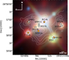 |
Fig. 1 Three-colour image of the Coronet cluster (WISE 3.4 µm, blue, 4.6 µm, green, and 12 µm, red, bands; Wright et al. 2010) overlaid with the SCUBA 850 µm density flux from Nutter et al. (2005); contours are in decreasing steps starting at the peak flux (3.7 Jy beam−1) and subtracting 30% from the previous level. The white stars mark the positions of Class 0/I YSOs in the Coronet region (Peterson et al. 2011; Nutter et al. 2005), whereas the orange stars indicate the Herbig Ae/Be star R CrA and the T Tauri star T CrA. The pre-stellar core candidate SMM1A is indicated with an orange circle and the orange square represents the Herbig Haro object HH100. |
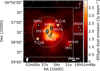 |
Fig. 2 SMA continuum at 1.3 mm (contours) overlaid with SCUBA 850 µm density flux from Nutter et al. (2005). The contours start at 5σ and continue in steps of 5σ (σ = 18 mJy beam−1). The empty circle indicates the size of the SMA primary beam, whereas the SMA synthesised beam is shown with a white ellipse in the bottom left corner. The empty rectangle shows the map covered by APEX observations. The stars mark the position of the objects located in the Coronet cluster; refer to Table 1 for their identification. |
2 Observations
The Coronet cluster was observed with the SMA (Ho et al. 2004) on February 25, 2020, April 28, 30, and May 19, 31, 2021 in the compact configuration, resulting in projected baselines between 17−72 m. The region was covered by one pointing centreed on IRS7B with coordinates αJ2000 = 19h01m56s;40, δJ2000 = −36°57′27.″00 (Fig. 2). The SWARM correlator provided a total frequency coverage of 36 GHz, with the lower sideband covering frequencies from 210.3 to 228.3 GHz and upper sideband from 230.3 to 248.3 GHz. The spectral resolution was 0.6 MHz corresponding to 0.7 km s−1.
Data calibration and imaging were performed with the CASA v. 5.7.2 package1 (McMullin et al. 2007; Bean et al. 2022). The complex gains were calibrated through observations of the quasars 1924-292 and 1957-387 and the bandpass through observations of the bright quasar 3C279. The overall flux calibration was carried out through observations of Vesta and Callisto. Imaging was done using the tclean algorithm and a Briggs weighting with a robust parameter of 0.5. The typical synthesised beam size of the SMA dataset was 4.″9 × 2.″6 (400–700 AU). The position angle (PA) for CH3OH, our main molecule of interest, at 241.791 GHz was −8.2°. The PA varies of ≈4.5º across the covered frequencies.
Additional information on the CH3OH large-scale emission towards the Coronet cluster was provided by observations with APEX (Güsten et al. 2006) during the nights of October 25-November 4, 2020. The pointing was the same as reported for the SMA observations. The achieved map size is 150″ × 150″, fully covering the region observed by the SMA. The frequencies probed by the APEX observations are in the range 235.1–243 GHz, corresponding to the SMA upper side band observations, with a frequency resolution of 0.061 MHz (0.076 km s−1). The resulting beam-size of the observations is 27.4″ for CH3OH. Data reduction was carried out with the GILDAS package CLASS2. Subsequently, the reduced APEX and SMA datasets were combined in CASA v. 5.7.2 using the feathering technique, following the procedure presented in Appendix B.1. of Perotti et al. (2020). The combination of SMA and APEX short-spacing data resulted in mapping the outer regions of protostellar envelopes in the Coronet cluster on scales from ~400–10 000 AU.
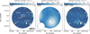 |
Fig. 3 Primary beam corrected integrated intensity maps for CH3OH J = 50−40 A+ transition (Eu = 34.8 K) at 241.791 GHz detected by the SMA (a), by the APEX telescope (b), and in the combined interferometric SMA and single-dish APEX data (c). All lines are integrated between 6 and 12.5 km s−1. Contours start at 5σ (σSMA= 0.16 Jy beam−1 km s−1, σAPEX= 2 Jy beam−1 km s−1, σSMA+APEX = 0.17 Jy beam−1 km s−1 ) and follow in steps of 5σ. The circular field-of-view corresponds to the primary beam of the SMA observations. The synthesised beams are displayed in white in the bottom left corner of each panel. |
3 Results
Figure 2 displays the region targeted by the SMA and APEX observations. The positions of the SMA 1.3 mm continuum peaks coincides with the location of the young stellar objects in the Coronet cluster. The strongest emission is observed towards the two Class 0 sources SMM1C and IRS7B and the Class I objects SMM2 and IRS7A. Fainter emission north of the prestellar core candidate SMM1A (Chen & Arce 2010) is also seen. Apart from the continuum, line emission of seven species was identified (Table A.1). These results are presented and discussed in Appendix A (Figs. A.1–A.3). In the remainder of this section we uniquely focus on the observed methanol (CH3OH) emission, our molecule of interest.
Amongst the molecular species detected in the Coronet cluster, methanol is the most suited for the main aim of this work: assessing the effect of external irradiation on the gas-phase and solid-state (ice) chemistries in the outer regions of protostellar envelopes. These are the regions probed in the presented SMA and APEX observations, at radii r > 400 AU from the protostar. Here, gas-phase methanol is not thermally desorbed and it is a tracer of energetic input such as outflows releasing frozen CH3OH to the gas phase (e.g. Tychoniec et al. 2021). The latter is due to the fact that the most efficient methanol formation pathway in star-forming regions (AV > 9 mag) occurs on ice-coated dust grains (Watanabe & Kouchi 2002; Fuchs et al. 2009; Simons et al. 2020; Santos et al. 2022). Consequently, the observed non-thermal CH3OH emission in the outer regions of protostellar envelopes does not trace the bulk of the ices, and instead, it probes a fraction of CH3OH ice sputtered in outflows or photodesorbed (see Kristensen et al. 2010 for an observational overview of CH3OH non-thermal desorption processes).
Figure 3 presents primary beam corrected integrated intensity (moment 0) maps of the CH3OH J = 50−40 A+ line for the SMA, APEX, and the combination of interferometric and single-dish data (SMA+APEX). The combined moment 0 maps of the other CH3OH transitions belonging to the J = 5K−4K Q-branch are displayed in Fig. A.2. We specifically targeted this branch because its multiple transitions are conveniently observable in a narrow spectral range (0.2 GHz; Table 2) and they are associated to Eu from 34.8 to 60.7 K, well below the typical CH3OH sublimation temperature as inferred from both observations and laboratory experiments (70–130 K; e.g. Kristensen et al. 2010; Penteado et al. 2017). The latter condition has to be satisfied in order to investigate methanol non-thermal desorption processes. Additionally, observations of CH3OH J = 5K−4K Q-branch make it possible to directly compare our results with previous work on CH3OH gas-to-ice ratios in nearby star-forming regions using the same facilities, observational strategy, and spectral setups (Perotti et al. 2020, 2021).
By looking at the SMA moment 0 map (Fig. 3; panel a), it is clear that the interferometric observations do not sufficiently recover the spatially extended emission originating from the Coronet cluster. In contrast, they filter out ≈90% of the extended emission detected in the APEX data. Unlike for the other species detected in the SMA data, we here want to perform a quantitative analysis of the CH3OH emission therefore, we combine the SMA data with the APEX map to avoid underestimating the CH3OH column densities by up to one order of magnitude.
Similarly to the CH3OH J = 42−31 E transition (Fig. A.2; panel g), the CH3OH J = 50−40 A+ emission is tracing the condensations associated to the prestellar core candidate SMM1A. The emission is extended in the APEX map (Fig. 3; panel b), and confined to two main regions, around SMM1A and to the east of SMM2. The peak intensity is observed also in this case in the vicinity of SMM1A. The same pattern is visible in the SMA + APEX moment 0 map (Fig. 3; panel c), but some CH3OH emission is also present at the SMM2, IRS7A, and IRS7B source positions although approximately a factor of 4 fainter compared to the peak position.
The CH3OH column densities towards the Coronet cluster members were determined from the integrated line intensities of the feathered SMA + APEX maps for all five CH3OH transitions belonging to the J = 5K−4K branch (Fig. A.2 and Table B.1). The spectra are shown in Fig. B.1. For column density calculations, we followed two different treatments: a local thermodynamic equilibrium (LTE) analysis, assuming optically thin emission (Goldsmith & Langer 1999), and a non-LTE study employing the RADEX code (van der Tak et al. 2007). For both methods, a temperature of 30 K is assumed (Lindberg & Jørgensen 2012). Although the non-LTE analysis indicates that the CH3OH lines are not thermalised (see Fig. B.3) for densities below 107 cm−3, and four out of five transitions are optically thick (see Fig. B.4), the estimated CH3OH column densities derived with both methods agree with each other (for typical envelope densities  between 105 and 106 cm−3; see Table B.2). More details about the LTE and non-LTE analysis are presented in Appendix B. Table 3 lists the resulting column densities calculated from the LTE analysis and using Trot = 30 K. The uncertainties were calculated from the spectral rms noise and 20% calibration uncertainty.
Identified methanol transitions in the SMA and APEX datasets.
Total ice and gas column densities (N) and fractional abundances (X) relative to H2 towards the Coronet cluster members.
4 Linking methanol ice and gas
In this section, we analyse the gas-ice variations in the Coronet cluster. The H2O and CH3OH ice column densities were determined by Boogert et al. (2008) from Spitzer IRS mid-infrared spectra as part of the Spitzer Legacy Program 'From Molecular Cores to Planet-Forming Disks’ (c2d). For the gas-phase counterpart, we made use of CH3OH gas column densities calculated in Sect. 3 and reported in Table 3.
4.1 H2 column densities
Prior to searching for gas-ice correlations, the physical structure of the Coronet cluster is investigated by producing an H2 column density map of the targeted region. This step is required as fractional abundances instead of absolute column densities need to be compared when studying gas-ice variations. This is due to the fact that gas and ice observations, by their very nature, are tracing different spatial scales, and therefore, a comparison between absolute values can lead to misinterpretations (e.g. Noble et al. 2017). At the same time we note that the H2 column density calculated below provides the total H2 column density – and hence it traces regions where methanol is in the gas phase as well in the ices. As a result, the CH3OH abundances presented in this work have to be interpreted as average abundances.
Figure 4 shows the H2 column density map of the Coronet cluster obtained by making use of SCUBA sub-millimetre continuum maps at 850 µm from Nutter et al. (2005). A detailed description of the formalism adopted to obtain the H2 column density from SCUBA maps is provided in Appendix C of Perotti et al. (2020). Briefly, in an optically thin thermal dust emission regime, the strength of the sub-millimetre radiation depends on the column density (N), the dust temperature (T) and the opacity (κν), (Kauffmann et al. 2008). The inserted value for the opacity per unit dust+gas mass is 0.0182 cm2 g−1 (‘OH5 dust’; Ossenkopf & Henning 1994). The adopted value for the dust temperature is 30 K, based on previous observational studies of the Coronet cluster and radiative transfer models by Lindberg & Jørgensen (2012).
The youngest cluster members are all situated in the densest areas of the targeted region (Fig. 4). The apex of the estimated H2 column density lies to the south-east of R CrA, and in particular at the IRS7B, SMM1A, SMM1C and IRS7A positions ( ). SMM2, IRS1, IRS5N and IRS5A are located in slightly less dense regions (
 ). The measured H2 column densities and their uncertainties for individual sources are listed in Table 3.
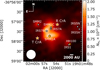 |
Fig. 4 H2 column density map of the R CrA region calculated from SCUBA dust emission maps at 850 µm by Nutter et al. (2005). Refer to Fig. 1 for a guide to the symbols of the Coronet cluster objects. |
4.2 Gas-ice variations
The analysis of gas-ice variations in the Coronet cluster is addressed by comparing fractional abundances (X) of gas and ice species relative to H2 (Table 3). In addition, this section also provides an overview of gas-ice variations in Coronet with respect to two other nearby low-mass star-forming clusters: Serpens SVS 4 and Orion B35A, which have been observed with the same facilities, angular resolution, and receiver settings adopted for observations of the Coronet cluster to assure a meaningful comparison and reduce observational bias (see Perotti et al. 2020, 2021).
Figure 5 displays CH3OH gas abundances as function of H2O (a) and CH3OH ice (b). A correlation between CH3OH gas and H2O ice for the three star-forming regions is seen in panel a with the Coronet cluster showing gas-ice abundances as low as the Orion B35A cloud. The lower methanol gas abundances in the Coronet cluster and in Orion B35A may be due to reduced ice mantle formation and enhanced photodissociation of methanol molecules upon desorption in these two regions with stronger UV field (see Sect. 5 for more details). The spread among the H2O abundances for the Coronet cluster and Orion B35A is limited, spanning less than a factor of 2.6 including the uncertainties. The same applies to the CH3OH gas abundances. In contrast, Serpens SVS 4 exhibits the highest values compared to the other two regions and the largest spread, with CH3OH gas abundances ranging up to ~20 × 10−8. One outlier is identified, Serpens SVS 4–12, which is characterised by the lowest CH3OH gas and highest H2O ice abundances relative to the other Serpens SVS 4 protostars. This result is not surprising since this is the most extincted object of all targeted sources (AV ~ 95 mag; Pontoppidan et al. 2004) with the lowest S/N (see Perotti et al. 2020 for a detailed discussion on Serpens SVS 4-12).
Figure 5b compares CH3OH gas and ice abundances. In contrast to panel a, no clear trend is seen. However, when Serpens SVS 4–12 is excluded from the analysis it is possible to identify three different groups corresponding to the three regions: (i) Orion B35A with the lowest measurements of both CH3OH in the gas and in the solid state; (ii) Serpens SVS 4 with intermediate to high values of CH3OH ice and the highest gas abundances, and finally (iii) the Coronet cluster, with some of the highest CH3OH ice but surprisingly low CH3OH gas abundances. The observed behaviour for the Coronet cluster is likely due to CH3OH destruction in the gas phase as a consequence of strong external irradiation (Lindberg & Jørgensen 2012).
Figure 6 shows H2O (a) and CH3OH (b) ice column densities (N) as function of cloud visual extinction (AV) for lines of sights in the three nearby star-forming clusters. The cloud extinction estimates were taken from Pontoppidan et al. (2004) for Serpens SVS 4, from Perotti et al. (2021) for Orion B35A, and from Alves et al. (2014) for the Coronet cluster, then converted to visual extinction using the conversion factors (3.6 for AJ, 5.55 for AH and 8.33 for AK) from Weingartner & Draine (2001) for RV = 5.5 for the dense ISM.
The distribution of data points in panels a and b shows a positive trend for Serpens SVS 4 and Orion B35A, indicating that to higher visual extinctions correspond higher columns of H2O (a) and CH3OH (b). This observation is particularly valid for H2O but it also applies to CH3OH when an evaluation is done per star-forming region. The opposite behaviour is found for the Coronet cluster members, for both ice species. This negative trend could simply reflect inaccurate extinction values due to the lack of background stars in the densest area of the Corona Australis complex, where the Coronet cluster members are located (see Sect. 2 of Alves et al. 2014 for more details).
5 Discussion
In this study, the CH3OH chemical behaviour has been investigated with millimetric and infrared facilities. This provides direct observational constraints on the CH3OH gas-to-ice ratio in protostellar envelopes and on its dependency on the physical conditions of star-forming regions. Laboratory experiments predict that CH3OH ice in cold dark clouds is non-thermally desorbed with an efficiency spanning over approximately three orders of magnitude (10−6−10−3 molecules/photon; Öberg et al. 2009b; Bertin et al. 2016; Cruz-Diaz et al. 2016; Martín-Doménech et al. 2016). This range is expected to increase up to ~10−2 molecules/photon (Basalgète et al. 2021a,b), as X-rays emitted from the central YSO strongly impact the abundances of CH3OH in protostellar envelopes (Notsu et al. 2021). Generally, the majority of non-thermally desorbed CH3OH molecules fragment during the desorption and a fraction of those recombine (e.g. Bertin et al. 2016). The CH3OH non-thermal desorption efficiency and by inference the gas-to-ice ratio is highly dependent on the ice structure and composition (pure CH3OH versus CH3OH mixed with CO molecules), as well as on the temperature, photon energy and flux (e.g. Öberg 2016; Carrascosa et al. 2023). To support laboratory experiments and computations, in this paper we provide observational measurements of the CH3OH gas-to-ice ratio in the outer regions of protostellar envelopes.
Our targeted regions (Serpens SVS 4, Orion B35A and Corona Australis Coronet) share a number of similarities: they are low-mass star-forming regions, they are clustered and finally, they are affected by the presence of outflows and/or Herbig-Haro objects. However, they show distinct physical conditions for instance, the Serpens SVS 4 cluster is influenced by the presence of the Class 0 binary SMM4 (Pontoppidan et al. 2004), whereas B35A is affected by the nearby high-mass star λ Orionis (Reipurth & Friberg 2021) and the Coronet is strongly irradiated by the Herbig Ae/Be star R CrA (Lindberg & Jørgensen 2012). B35A is exposed to an interstellar radiation field,χISRF of 34 (Wolfire et al. 1989)3 enhanced by the neighbouring λ Orionis (Dolan & Mathieu 2002), whereas the radiation field in the Coronet cluster has been estimated to approximately, YISRF ~750 to account for the high fluxes at millimetre wavelengths (Lindberg & Jørgensen 2012).
In addition, the molecular clouds in which our targeted regions are located do not share a common formation history. The ongoing low-mass star formation in Serpens Main might have been triggered by cloud-cloud collisions (Duarte-Cabral et al. 2010) or compression from a shock wave from a supernova. However, there is no clear evidence that a nearby supernova ever occurred (Herczeg et al. 2019). In contrast to Serpens, the formation of the ring constituting the λ Orionis region is attributed to a supernova explosion that occurred roughly 1–6 Myr ago (Dolan & Mathieu 1999, 2002; Kounkel 2020). The low-mass star formation in B35A was likely generated by the presence of neighbouring massive stars and their stellar winds (Barrado et al. 2018). Finally, star formation in CrA has been supposedly promoted by a high-velocity cloud impact onto the Galactic plane (Neuhäuser & Forbrich 2008) or by the expansion of the UpperCenLupus (UCL) superbubble (Mamajek et al. 2002). The fact that the three regions likely did not form in the same way implies different initial physical conditions for the production of CH3OH.
Figure 7 illustrates the distribution of the CH3OH gas-to-ice ratios (Ngas/Nice) towards low-mass protostars located in the different molecular clouds described above. The average CH3OH gas-to-ice ratio (1.2 × 10⁻⁴) determined from millimetric (single-dish) and infrared measurements by Öberg et al. (2009a) for four Class 0/I sources in Perseus, Taurus and Serpens is over-plotted. A detailed comparison between the gas-to-ice ratio determined by Öberg et al. (2009a) and the ratios calculated for the sources in the Serpens SVS 4 and the Orion B35A cloud is provided in Perotti et al. (2021). In this section we focus on the ratios obtained for CrA and their comparison with the values determined for the two other star-forming regions.
The distribution of CH3OH gas-to-ice ratios towards the Coronet cluster covers approximately one order of magnitude. The uncertainty on the determination of the CH3OH ice column densities for HH100 IRS1 and IRS7A (Boogert et al. 2008) results in lower limits for their gas-to-ice ratios, consequently we cannot provide solid comparisons for these two sources. In contrast, the values obtained for IRS5A and IRS7B fall in the range of gas-to-ice ratios previously obtained for the protostars located in the Serpens SVS 4 cluster.
The CH3OH gas-to-ice ratios constrained from gas and ice observations of a sample of protostellar envelopes (Fig. 7) do not point to one value but, instead, to a distribution (from 1.2 × 10⁻⁴ to 3.1 × 10⁻³) which validates previous observational studies (e.g. Öberg et al. 2009a; Perotti et al. 2020). This distribution agrees with a more complex scenario for the CH3OH desorption elucidated in the laboratory in which a large fraction of CH3OH molecules do not desorb intact, but instead fragment and eventually recombine during and after the desorption (e.g. Bertin et al. 2016) leading to CH3OH gas-to-ice ratios lower than 10−3.
A second interesting observation is that the CH3OH gas-to-ice ratios fall in a fairly narrow range; this suggests that the CH3OH chemistry at play in the cold outer regions of protostellar envelopes belonging to different low-mass star-forming regions is relatively independent of variations in the physical conditions. We note that a similar conclusion could not be tested for the innermost envelope regions where thermal desorption dominates and young discs are present; our observations are simply not sensitive to these regions. Our analysis implicitly indicates that the CH3OH chemistry in the outer envelope regions is set to a large degree already during the prestellar stage. A related result came to light when comparing abundances of complex organic molecules observed in distinct star-forming environments Scibelli & Shirley (2020), (e.g. Galactic disc versus Galactic centre, high-mass versus low-mass star-forming region; Jørgensen et al. 2020; Coletta et al. 2020; Yang et al. 2021; Nazari et al. 2022a). A larger sample is however necessary to prove this statement, and additional observations, laboratory experiments and modelling efforts are required to elucidate further the impact of the physical evolution of protostars on their chemical signatures and vice versa.
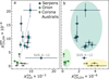 |
Fig. 5 Relationship between CH3OH and H2O fractional abundances (X) towards three nearby low-mass star-forming regions. The triangles represent the gas and ice fractional abundances relative to H2 for the Coronet cluster members listed in Table 3 for which both gas and ice measurements are available. The squares and circles symbolise the values obtained for Serpens SVS 4 and Orion B35A from Perotti et al. (2020, 2021), respectively. The CH3OH gas abundances are compared to the H2O (panel a) and CH3OH (panel b) ice abundances. Upper limits are marked as empty arrows. The grey line in panel a represents the linear fit to the detections. In panel b three different groups are identified, excluding Serpens SVS 4–12; they correspond to the three star-forming regions and they are marked with coloured ovals. |
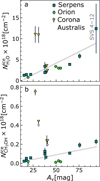 |
Fig. 6 Relationship between H2O (a), CH3OH (b) ice column densities (N) and visual extinction (AV) for lines of sights in nearby star-forming clusters: Corona Australis Coronet (triangles), Serpens SVS 4 (squares), and Orion B35A (circles). Upper limits are marked as arrows. The grey lines represent linear fits to the detections. We note that the visual extinction values obtained for CrA have to be taken with care as their determination is hampered by the lack of background stars towards the densest region of the Coronet cluster (see Sect. 4.2). The data for Serpens SVS 4 and Orion B35A were taken from Perotti et al. (2020, 2021), respectively. |
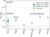 |
Fig. 7 CH3OH gas-to-ice ratios (Ngas/Nice) towards low-mass protostars in the Coronet cluster in Corona Australis (triangles). The square and the circle symbolise the average ratios for ten sources in Serpens SVS 4 and four sources in Orion B35A, respectively. The green shaded area corresponds to the interval of gas-to-ice ratios observed for the ten sources in the Serpens SVS 4 cluster. The dotted line indicates the average value for four sources from Öberg et al. (2009a). Upper and lower limits are marked as arrows. |
6 Conclusions
We present 1.3 mm SMA and APEX observations towards the Coronet cluster in Corona Australis, a unique astrochemical laboratory to study the effect of external irradiation on the chemical and physical evolution of young protostars. In addition, we determined CH3OH gas-phase abundances and compared those with CH3OH ice abundances from Boogert et al. (2008) to directly constrain the CH3OH gas-to-ice ratio in cold protostellar envelopes. Our key findings are:
We find a positive trend between H2O ice and CH3OH gas abundances in Serpens SVS 4, Coronet, and Orion B35A with the latter two regions showing the lowest gas abundances. This result is attributed to reduced ice mantle formation and substantial destruction of methanol gas molecules in these two regions characterised by stronger external UV field;
The distribution of CH3OH gas-to-ice ratios in CrA constrained from millimetric and infrared observations spans approximately one order of magnitude (from 1.2 × 10⁻⁴ to 3.1 × 10⁻³) and reinforces previous observational constraints on the CH3OH gas-to-ice ratio;
Similarities are found between CH3OH gas-to-ice ratios determined in different low-mass star forming regions (Serpens SVS 4, Orion B35A and Corona Australis Coronet), characterised by distinct physical conditions and formation histories. This result suggests that the CH3OH chemistry – in the outer regions of low-mass envelopes – is relatively independent of variations in the physical conditions and thus it is set to a large degree during the prestellar stage.
Multiple avenues for future studies can be pursued. Comparisons of gas and ice abundances of key species are currently limited by the low number of infrared surveys. Current infrared facilities such as the James Webb Space Telescope are now routinely probing interstellar ices towards background stars (McClure et al. 2023), pre-stellar cores, proto-stellar envelopes (Yang et al. 2022) and near edge-on discs (Sturm et al. 2023), thus significantly increasing the number of studied regions. Therefore, it will be feasible to search for gas-ice trends found in other regions, improve our constraints on the CH3OH gas-to-ice ratios, and ultimately determine ratios for a larger set of major interstellar molecules. This approach will provide important feedback on the interactions between ice and gas material during its journey from the molecular cloud to the disc and on the impact of the physical conditions on the physico-chemical evolution of protostars. In this context, the Corona Australis complex still has much to teach us, hosting one of the youngest population of protostars observed so far.
Acknowledgements
We thank Chunhua Qi for translating the SMA data into a format readable in CASA, Henrik Olofsson, and Dirk Petry for guidance in importing the APEX data to CASA and the anonymous reviewer for the careful reading of the manuscript and the useful comments. This work is based on observations with the Submillimeter Array, Mauna Kea, Hawaii, program codes: 2019B-S014 and 2020B-S058 (PI: Perotti) and with the Atacama Pathfinder Experiment, Llano Chajnantor, Chile, program code: 0105.F-9300 (PI: Perotti). The Submillimeter Array is a joint project between the Smithsonian Astro-physical Observatory and the Academia Sinica Institute of Astronomy and Astrophysics and is funded by the Smithsonian Institution and the Academia Sinica. The Atacama Pathfinder Experiment (APEX) telescope is a collaboration between the Max Planck Institute for Radio Astronomy, the European Southern Observatory, and the Onsala Space Observatory. Swedish observations on APEX are supported through Swedish Research Council grant No 2017-00648. This publication also makes use of data products from the Wide-field Infrared Survey Explorer, which is a joint project of the University of California, Los Angeles, and the Jet Propulsion Laboratory/California Institute of Technology, funded by the National Aeronautics and Space Administration. GP gratefully acknowledges support from the Max Planck Society. The research of MS is supported by NASA under award number 80GSFC21M0002. JKJ acknowledges support from the Independent Research Fund Denmark (grant number 0135-00123B). EAdlV acknowledges financial support provided by FONDECYT grant 3200797. HJF gratefully acknowledges the support of STFC for Astrochemistry at the OU under grant Nos ST/P000584/1 and ST/T005424/1 enabling her participation in this work. SBC was supported by the NASA Planetary Science Division Internal Scientist Funding Program through the Fundamental Laboratory Research work package (FLaRe). The authors wish to recognise and acknowledge the very significant cultural role and reverence that the summit of Mauna Kea and the Atacama desert have always had within the indigenous Hawaiian and Atacama communities. We are most fortunate to have the opportunity to conduct observations from both sites.
Appendix A Overview of molecular line detections
This section reports the primary beam corrected integrated intensity (moment zero) maps of the species detected in the SMA dataset (Figures A.1–A.3). For our molecule of interest, CH3OH, we also include in A.2 the combined SMA+APEX integrated intensity maps. Please refer to Appendix B.1 of Perotti et al. (2020) for a detailed description of the feathering procedure used to combine interferometric and single-dish data.
The eighteen molecular transitions of seven species identified in the SMA datasets are listed in Table A.1. The detected species are: carbon monoxide (12CO, 13CO and C18O), formaldehyde (H2CO), methanol (CH3OH), sulphur oxide (SO), sulphur dioxide (SO2), cyclopropenylidene (c-C3H2), and cyanoacetylene (HC3N). The line emission is predominantly extended and it does not necessarily coincide with the position of the compact continuum sources in the Coronet cluster (Figures A.1–A.3). In contrast, it is mostly localised to the east of the Herbig Ae/Be star R CrA and to the south of the young stellar objects IRS7A and IRS7B, at the pre-stellar core SMM1A position. This statement applies especially to H2CO and CH3OH, and is consistent with previous 1.3 mm SMA observations of the region by Lindberg & Jørgensen (2012) covering the 216.849–218.831 GHz and 226.849–228.831 GHz frequencies ranges. Interestingly, no molecular line emission was detected towards SMM1A in the SMA dataset presented by Chen & Arce (2010), although the same number of antennas and configuration were used and the SMA correlator covered spectral ranges similar to the ones presented in this work. However, the SMA observations by Chen & Arce (2010) were designed to study the dust continuum and they were characterised by a shorter bandwidth and likely lower line sensitivity. Unfortunately, a comparison of the line sensitivity of the two datasets could not be made as this information is not reported in Chen & Arce (2010) and a reduced, continuum-subtracted spectrum is not provided either.
The detected species in the SMA data can be roughly divided into three groups described based on their emission pattern (Table A.1): (I) CO species, (II) S-species, and (III) carbon-chain species. Overall, the emission reported in the SMA dataset is dominated by molecular tracers such as H2CO, CH3OH, SO, SO2. The emission of H2CO and CH3OH is consistent with temperature variations in the field of view of the observations, and particularly with the external irradiation from the variable stars in the region (R CrA and T CrA). In contrast, the shock tracers (SO, SO2) probe the numerous outflows and Herbig-Haro objects in the region, which are indicators of a young stellar population in the earliest evolutionary stages.
Appendix A.1 CO species
Figure A.1 displays the SMA primary beam corrected integrated intensity maps for 12CO, 13CO, C18O and H2CO. The distribution of the CO-species emission is extended, especially for 12CO and its isotopologues. The three transitions of H2CO show the same emission pattern (Figure A.1, panels d–f). The emission is localised in two ridges: the northern ridge between R CrA and SMM1C, and the southern ridge to the south of IRS7B, in the vicinity of SMM1A. No bright line emission is observed towards the young stellar objects SMM1C, IRS7A and IRS7B. The emission offset from the YSO positions and the elongated shape of the ridges have been previously identified in this region and interpreted as indicators of external heating (Lindberg & Jørgensen 2012). The emission localised in the southern ridge traces the three condensations within the pre-stellar core SMM1A (SMM1A-a, SMM1A-b, and SMM1A-c), analysed in dust continuum observations by Chen & Arce (2010).
The strength of the H2CO emission, for the three detected H2CO lines is comparable in both ridges. A similar morphology pattern is observed for CH3OH where the emission peak is located within the SMM1A core. However, neither the CH3OH J=42 − 31 line nor the CH3OH transitions belonging to the J = 5K − 4K branch show a northern ridge (Figures 3 and A.2).
Appendix A.2 S species
The SO and SO2 line emissions appear relatively bright and compact (Figure A.3, panels m–o). The distribution of the emission is identical for the two SO transitions, and it peaks towards IRS7A and SMM1C. The strength of the emission among the SO transitions is very similar (7–8 Jy beam−1 km s−1; Figure A.3, panels m–n). The SO2 emission is concentrated towards IRS7A and is approximately a factor of 2.5 fainter compared to SO (Figure A.3, panels o). In contrast to the majority of the CO-species, the S-species emission have their strongest emission associated with the YSO positions. SO and SO2 are molecular tracers of energetic inputs in the form of outflows and jets. The luminous SO and SO2 emissions appear to indicate that higher velocity (~5–10 km s−1) flows of matter are present in the field-of-view of the observations, associated with IRS7A and SMM1C. This result is in agreement with studies of the Herbig-Haro objects in the Coronet cluster attributed to SMM1C (Wang et al. 2004; Peterson et al. 2011).
Appendix A.3 Carbon-chain species
The third group of lines corresponds to carbon-chain species such as c-C3H2 and HC3N which show a fairly weak emission (1.6–3.0 Jy beam−1 km s−1) compared to the previous two groups (CO- and S-species). Their emission is diffuse and characterised by a fairly low S/N (Figure A.3, panels p-r). Similarly to 13CO and C18O, the carbon-chain species have their brightest emission associated with IRS7B.
Identified molecular transitions in the SMA dataset.
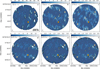 |
Fig. A.1 Primary beam corrected integrated intensity maps in Jy beam−1km s−1 for the different species detected with the SMA. In each plot contours start at 5σ and continue in intervals of 5σ, except for panel a-c for which contours start at 10σ and continue in intervals of 10σ. Shown are (a) CO J = 2 − 1 (σ= 0.96 Jy beam−1km s−1), (b) 13CO J = 2 − 1 (σ= 0.32 Jy beam−1km s−1 ), (b) C18O J = 2 − 1 (σ= 0.13 Jy beam−1km s−1), (d) H2CO 303 − 202 (σ= 0.23 mJy beam−1km s−1), (e) H2CO 321−220 (σ= 88 mJy beam−1km s−1), (f) H2CO 322 − 221 (σ= 0.14 mJy beam−1km s−1). The circular field-of-view corresponds to the SMA primary beam. The size of the synthesised beam is shown in the lower left corner of each image. The white and orange stars and the orange circle mark the position of the Coronet cluster members as in Fig. 1. |
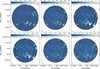 |
Fig. A.2 Same as Figure A.1, but for primary beam corrected integrated intensity maps in Jy beam−1km s−1 for: (g) CH3OH 42−31 (σ= 88 mJy beam−1km s−1), (h) CH3OH 5+0−4+0 E (σ= 0.12 Jy beam−1km s−1), (i) CH3OH 5−1−4−1 E (σ=0.13 Jy beam−1km s−1), (j) CH3OH 50−40 A+ (σ= 0.17 Jy beam−1km s−1), (k) CH3OH 5+1−4+1 E (σ= 0.13 Jy beam−1km s−1), and (1) CH3OH 5−2−4−2 E (σ= 0.15 mJy beam−1km s−1) detected by the SMA (panel g), and in the combined SMA and APEX data (panels h-1). |
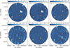 |
Fig. A.3 Same as Figure A.1, but for primary beam corrected integrated intensity maps in Jy beam−1km s−1 for : (m) SO 55 − 44 (σ= 0.12 Jy beam−1km s−1), (n) SO 65 − 54 (σ= 0.13 Jy beam−1km s−1), (o) SO2 422 − 313 (σ= 0.15 Jy beam−1km s−1), (p) c-C3H2 606 − 515 (σ= 0.13 Jy beam−1km s−1), (q) c-C3H2 514 −423 (σ= 0.11 Jy beam−1 km s−1), and (r) HC3N J = 24 − 23 (σ= 71 mJy beam−1km s−1) detected by the SMA. |
Appendix B Gas-phase methanol
Appendix B.1 Spectra of methanol
Figure B.1 shows the spectra for the brightest transitions of the CH3OH JK = 5K – 4K Q-branch, J=50 − 40 A+ and J=5−1−4−1 E, respectively, extracted from the combined SMA + APEX dataset. Table A.1 reports the spectral data for both CH3OH transitions. The CH3OH emission lines have a Gaussian shape and do not show blue or red-shifted components.
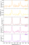 |
Fig. B.1 CH3OH J=50−40 A+ and CH3OH J=5−1−4−1 E spectra towards the Coronet cluster members detected in the combined SMA+APEX dataset. |
Appendix B.2 Derivation of CH3 OH column densities
The column densities of gas-phase CH3OH for the Coronet cluster members were calculated using the integrated intensities of the combined interferometric (SMA) and single-dish (APEX) data reported in Table B.1. The SMA+APEX primary beam corrected integrated intensity (moment 0) maps for the CH3OH JK = 5K − 4K Q-branch are displayed in Figure A.2.
For the column density calculation one of the two adopted procedures assumes LTE conditions, optically thin line emission, homogeneous source filling the telescope beam and a single excitation temperature to describe the level population. The equations used follow the prescription of Goldsmith & Langer (1999), but assuming a fixed rotational temperature equal to 30 K (Lindberg & Jørgensen 2012), are reported in Appendix A.4 of Perotti et al. (2021) and thus they will not be repeated here. The values used for the column densities calculation are listed in Table 2 and have been compiled from the Cologne Database for Molecular Spectroscopy (CDMS; Müller et al. 2001, 2005; Endres et al. 2016) and the Jet Propulsion Laboratory catalogue (Pickett et al. 1998). In particular, the spectroscopic data are from Xu et al. (2008). The rotational diagrams for the Coronet cluster members are shown in Figure B.2. The CH3OH column densities and their uncertainties are reported in Table 3. Using a different rotational temperature (e.g. 20 K or 40 K) results in column densities being increased or decreased by approximately a factor of 0.5, respectively. The uncertainties on the gas column densities were calculated based on the spectral rms noise and on the 20% calibration uncertainty.
Appendix B.3 Non-LTE analysis
Further analysis of the CH3OH emission was performed using the non-LTE code RADEX (van der Tak et al. 2007). In particular, all the five CH3OH transitions were used to compare the observed relative intensities with the RADEX results for a H2 number density ( ) in the range 103 − 107 cm−3 and a kinetic temperature equal to 30 K. Figure B.3 shows that all lines are in sub-thermal regime for
  below 107 cm−3, typical for protostellar envelopes. Figure B.4 illustrates the optical depth of the five transitions for CH3OH column densities between 1013 − 1016 cm−2. The three brightest transitions (J = 5+0 − 4+0, J = 5−1 − 4−1, J = 50 − 40) are optically thick for CH3OH column densities equal to 1015 cm−2, while the J = 5+1 − 4+1 transition is marginally optically thick and the weakest transition, J = 5−2 − 4−2, can be considered as optically thin. Figures B.5–B.7 show a visual comparison between CH3OH column densities calculated using RADEX and obtained from the LTE analysis for each Coronet cluster member. Thin contours represent lower limits for the integrated line intensities of the optically thick lines from Table B.1, while thick contours indicate integrated line intensities for the less optically thick lines. The thickness of these contours are given by the errors of the integrated line intensities. A range of CH3OH column densities is estimated for each source from the weakest transition (CH3OH J = 5−2 − 4−2) and assuming
  between 105 and 106 cm−3 (see Table B.2). The vertical black line in Figures B.5–B.7 depicts the CH3OH column densities calculated with the LTE analysis listed in Table 3. We note that the column densities obtained with both methods are consistent for
  equal to 105 − 106 cm−3 (see Table B.2).
Integrated CH3OH line intensities in units of Jy beam−1 km s−1 towards the Coronet cluster members.
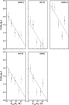 |
Fig. B.2 Rotational diagrams of CH3OH for the Coronet cluster members. The solid line shows the fixed slope for Trot = 30 K. Error bars are for 1σ uncertainties. The column densities are reported in Table 3. Only transitions belonging to the J = 5K − 4K Q-branch have been considered. |
Comparison between total CH3OH gas column densities (N) calculated using the LTE and the non-LTE analyses towards the Coronet cluster members.
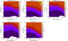 |
Fig. B.3 RADEX model results for the five CH3OH transitions (Table A.1) using Tkin = 30 K. The cyan line indicates Tex = 30 K. |
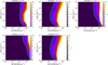 |
Fig. B.4 Optical depth for the five CH3OH transitions obtained with RADEX, using Tkin = 30 K. The cyan line represents τ = 1. |
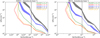 |
Fig. B.5 RADEX model results for the observed CH3OH lines towards SMM1C (left) and IRS7A (right), using Tkin = 30 K. Red, orange and green contours represent lower limits for the integrated line intensities of optically thick lines whereas blue and grey contours represent the marginally optically thin lines and include the errors from Table B.1. The vertical line is the CH3OH column density calculated assuming LTE conditions and optically thin emission reported in Table 3. |
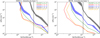 |
Fig. B.6 Same as Figure B.5, but for SMM1A (left) and IRS7B (right). |
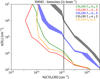 |
Fig. B.7 Same as Figure B.5, but for SMM2. |
References
- Alves, J., Lombardi, M., & Lada, C. J. 2014, A&A, 565, A18 [NASA ADS] [CrossRef] [EDP Sciences] [Google Scholar]
- Alves, F. O., Cleeves, L. I., Girart, J. M., et al. 2020, ApJ, 904, L6 [NASA ADS] [CrossRef] [Google Scholar]
- Andrews, S. M., Huang, J., Pérez, L. M., et al. 2018, ApJ, 869, L41 [NASA ADS] [CrossRef] [Google Scholar]
- Artur de la Villarmois, E., Kristensen, L. E., Jørgensen, J. K., et al. 2018, A&A, 614, A26 [NASA ADS] [CrossRef] [EDP Sciences] [Google Scholar]
- Balucani, N., Ceccarelli, C., & Taquet, V. 2015, MNRAS, 449, L16 [Google Scholar]
- Barrado, D., de Gregorio Monsalvo, I., Huélamo, N., et al. 2018, A&A, 612, A79 [NASA ADS] [CrossRef] [EDP Sciences] [Google Scholar]
- Basalgète, R., Dupuy, R., Féraud, G., et al. 2021a, A&A, 647, A35 [NASA ADS] [CrossRef] [EDP Sciences] [Google Scholar]
- Basalgète, R., Dupuy, R., Féraud, G., et al. 2021b, A&A, 647, A36 [EDP Sciences] [Google Scholar]
- Bean, B., Bhatnagar, S., Castro, S., et al. 2022, PASP, 134, 114501 [NASA ADS] [CrossRef] [Google Scholar]
- Bertin, M., Romanzin, C., Doronin, M., et al. 2016, ApJ, 817, L12 [NASA ADS] [CrossRef] [Google Scholar]
- Bibo, E. A., The, P. S., & Dawanas, D. N. 1992, A&A, 260, 293 [NASA ADS] [Google Scholar]
- Boogert, A. C. A., Pontoppidan, K. M., Knez, C., et al. 2008, ApJ, 678, 985 [Google Scholar]
- Boogert, A. C. A., Gerakines, P. A., & Whittet, D. C. B. 2015, ARA&A, 53, 541 [Google Scholar]
- Bottinelli, S., Boogert, A. C. A., Bouwman, J., et al. 2010, ApJ, 718, 1100 [NASA ADS] [CrossRef] [Google Scholar]
- Carrascosa, H., Satorre, M. Á., Escribano, B., Martín-Doménech, R., & Muñoz Caro, G. M. 2023, MNRAS, 525, 2690 [NASA ADS] [CrossRef] [Google Scholar]
- Cazzoletti, P., Manara, C. F., Baobab Liu, H., et al. 2019, A&A, 626, A11 [NASA ADS] [CrossRef] [EDP Sciences] [Google Scholar]
- Chen, X., & Arce, H. G. 2010, ApJ, 720, L169 [NASA ADS] [CrossRef] [Google Scholar]
- Chuang, K. J., Fedoseev, G., Ioppolo, S., van Dishoeck, E. F., & Linnartz, H. 2016, MNRAS, 455, 1702 [Google Scholar]
- Coletta, A., Fontani, F., Rivilla, V. M., et al. 2020, A&A, 641, A54 [NASA ADS] [CrossRef] [EDP Sciences] [Google Scholar]
- Cruz-Diaz, G. A., Martín-Doménech, R., Muñoz Caro, G. M., & Chen, Y.-J. 2016, A&A, 592, A68 [NASA ADS] [CrossRef] [EDP Sciences] [Google Scholar]
- Dib, S., & Henning, T. 2019, A&A, 629, A135 [NASA ADS] [CrossRef] [EDP Sciences] [Google Scholar]
- Dolan, C. J., & Mathieu, R. D. 1999, AJ, 118, 2409 [Google Scholar]
- Dolan, C. J., & Mathieu, R. D. 2002, AJ, 123, 387 [Google Scholar]
- Draine, B. T., & Bertoldi, F. 1996, ApJ, 468, 269 [Google Scholar]
- Duarte-Cabral, A., Fuller, G. A., Peretto, N., et al. 2010, A&A, 519, A27 [NASA ADS] [CrossRef] [EDP Sciences] [Google Scholar]
- Endres, C. P., Schlemmer, S., Schilke, P., Stutzki, J., & Müller, H. S. P. 2016, J. Mol. Spectrosc., 327, 95 [NASA ADS] [CrossRef] [Google Scholar]
- Esplin, T. L., & Luhman, K. L. 2022, AJ, 163, 64 [NASA ADS] [CrossRef] [Google Scholar]
- Fedoseev, G., Chuang, K. J., Ioppolo, S., et al. 2017, ApJ, 842, 52 [Google Scholar]
- Forbrich, J., & Preibisch, T. 2007, A&A, 475, 959 [NASA ADS] [CrossRef] [EDP Sciences] [Google Scholar]
- Forbrich, J., Preibisch, T., Menten, K. M., et al. 2007, A&A, 464, 1003 [NASA ADS] [CrossRef] [EDP Sciences] [Google Scholar]
- Fuchs, G. W., Cuppen, H. M., Ioppolo, S., et al. 2009, A&A, 505, 629 [NASA ADS] [CrossRef] [EDP Sciences] [Google Scholar]
- Galli, P. A. B., Bouy, H., Olivares, J., et al. 2020, A&A, 634, A98 [NASA ADS] [CrossRef] [EDP Sciences] [Google Scholar]
- Garrod, R. T., & Herbst, E. 2006, A&A, 457, 927 [NASA ADS] [CrossRef] [EDP Sciences] [Google Scholar]
- Geppert, W. D., Hamberg, M., Thomas, R. D., et al. 2006, Faraday Discuss., 133, 177 [Google Scholar]
- Goldsmith, P. F., & Langer, W. D. 1999, ApJ, 517, 209 [Google Scholar]
- Gray, R. O., Corbally, C. J., Garrison, R. F., et al. 2006, AJ, 132, 161 [Google Scholar]
- Groppi, C. E., Hunter, T. R., Blundell, R., & Sandell, G. 2007, ApJ, 670, 489 [CrossRef] [Google Scholar]
- Güsten, R., Nyman, L. Å., Schilke, P., et al. 2006, A&A, 454, L13 [NASA ADS] [CrossRef] [EDP Sciences] [Google Scholar]
- Harsono, D., Bjerkeli, P., van der Wiel, M. H. D., et al. 2018, Nat. Astron., 2, 646 [Google Scholar]
- Haworth, T. J., Kim, J. S., Winter, A. J., et al. 2021, MNRAS, 501, 3502 [NASA ADS] [CrossRef] [Google Scholar]
- Herbig, G. H. 1960, ApJS, 4, 337 [Google Scholar]
- Herczeg, G. J., Kuhn, M. A., Zhou, X., et al. 2019, ApJ, 878, 111 [NASA ADS] [CrossRef] [Google Scholar]
- Ho, P. T. P., Moran, J. M., & Lo, K. Y. 2004, ApJ, 616, L1 [Google Scholar]
- Jørgensen, J. K., Belloche, A., & Garrod, R. T. 2020, ARA&A, 58, 727 [Google Scholar]
- Kauffmann, J., Bertoldi, F., Bourke, T. L., Evans, N. J. I., & Lee, C. W. 2008, A&A, 487, 993 [NASA ADS] [CrossRef] [EDP Sciences] [Google Scholar]
- Keane, J. V., Tielens, A. G. G. M., Boogert, A. C. A., Schutte, W. A., & Whittet, D. C. B. 2001, A&A, 376, 254 [NASA ADS] [CrossRef] [EDP Sciences] [Google Scholar]
- Keppler, M., Benisty, M., Müller, A., et al. 2018, A&A, 617, A44 [NASA ADS] [CrossRef] [EDP Sciences] [Google Scholar]
- Kounkel, M. 2020, ApJ, 902, 122 [NASA ADS] [CrossRef] [Google Scholar]
- Kristensen, L. E., van Dishoeck, E. F., van Kempen, T. A., et al. 2010, A&A, 516, A57 [NASA ADS] [CrossRef] [EDP Sciences] [Google Scholar]
- Kuffmeier, M., Zhao, B., & Caselli, P. 2020, A&A, 639, A86 [NASA ADS] [CrossRef] [EDP Sciences] [Google Scholar]
- Lindberg, J. E., & Jørgensen, J. K. 2012, A&A, 548, A24 [NASA ADS] [CrossRef] [EDP Sciences] [Google Scholar]
- Lindberg, J. E., Jørgensen, J. K., Brinch, C., et al. 2014, A&A, 566, A74 [NASA ADS] [CrossRef] [EDP Sciences] [Google Scholar]
- Lindberg, J. E., Jørgensen, J. K., Watanabe, Y., et al. 2015, A&A, 584, A28 [NASA ADS] [CrossRef] [EDP Sciences] [Google Scholar]
- Mamajek, E. E., Meyer, M. R., & Liebert, J. 2002, AJ, 124, 1670 [Google Scholar]
- Martín-Doménech, R., Muñoz Caro, G. M., & Cruz-Díaz, G. A. 2016, A&A, 589, A107 [NASA ADS] [CrossRef] [EDP Sciences] [Google Scholar]
- McGuire, B. A. 2022, ApJS, 259, 30 [NASA ADS] [CrossRef] [Google Scholar]
- McClure, M. K., Rocha, W. R. M., Pontoppidan, K. M., et al. 2023, Nat. Astron., 7, 431 [NASA ADS] [CrossRef] [Google Scholar]
- McMullin, J. P., Waters, B., Schiebel, D., Young, W., & Golap, K. 2007, ASP Conf. Ser., 376, 127 [Google Scholar]
- Mesa, D., Bonnefoy, M., Gratton, R., et al. 2019, A&A, 624, A4 [NASA ADS] [CrossRef] [EDP Sciences] [Google Scholar]
- Miettinen, O., Kontinen, S., Harju, J., & Higdon, J. L. 2008, A&A, 486, 799 [NASA ADS] [CrossRef] [EDP Sciences] [Google Scholar]
- Müller, H. S. P., Thorwirth, S., Roth, D. A., & Winnewisser, G. 2001, A&A, 370, L49 [Google Scholar]
- Müller, H. S. P., Schlöder, F., Stutzki, J., & Winnewisser, G. 2005, J. Mol. Struct., 742, 215 [Google Scholar]
- Nazari, P., Meijerhof, J. D., van Gelder, M. L., et al. 2022a, A&A, 668, A109 [NASA ADS] [CrossRef] [EDP Sciences] [Google Scholar]
- Nazari, P., Tabone, B., Rosotti, G. P., et al. 2022b, A&A, 663, A58 [NASA ADS] [CrossRef] [EDP Sciences] [Google Scholar]
- Neuhäuser, R., & Forbrich, J. 2008, The Corona Australis Star Forming Region, 5 (Reipurth, B.), 735 [Google Scholar]
- Noble, J. A., Fraser, H. J., Pontoppidan, K. M., & Craigon, A. M. 2017, MNRAS, 467, 4753 [Google Scholar]
- Notsu, S., van Dishoeck, E. F., Walsh, C., Bosman, A. D., & Nomura, H. 2021, A&A, 650, A180 [NASA ADS] [CrossRef] [EDP Sciences] [Google Scholar]
- Nutter, D. J., Ward-Thompson, D., & André, P. 2005, MNRAS, 357, 975 [CrossRef] [Google Scholar]
- Öberg, K. I. 2016, Chem. Rev., 116, 9631 [Google Scholar]
- Öberg, K. I., Bottinelli, S., & van Dishoeck, E. F. 2009a, A&A, 494, L13 [NASA ADS] [CrossRef] [EDP Sciences] [Google Scholar]
- Öberg, K. I., Garrod, R. T., van Dishoeck, E. F., & Linnartz, H. 2009b, A&A, 504, 891 [NASA ADS] [CrossRef] [EDP Sciences] [Google Scholar]
- Ossenkopf, V., & Henning, T. 1994, A&A, 291, 943 [NASA ADS] [Google Scholar]
- Penteado, E. M., Walsh, C., & Cuppen, H. M. 2017, ApJ, 844, 71 [Google Scholar]
- Perotti, G., Rocha, W. R. M., Jørgensen, J. K., et al. 2020, A&A, 643, A48 [EDP Sciences] [Google Scholar]
- Perotti, G., Jørgensen, J. K., Fraser, H. J., et al. 2021, A&A, 650, A168 [NASA ADS] [CrossRef] [EDP Sciences] [Google Scholar]
- Peterson, D. E., Caratti o Garatti, A., Bourke, T. L., et al. 2011, ApJS, 194, 43 [NASA ADS] [CrossRef] [Google Scholar]
- Pickett, H. M., Poynter, R. L., Cohen, E. A., et al. 1998, J. Quant. Spec. Radiat. Transf., 60, 883 [Google Scholar]
- Pineda, J. E., Arzoumanian, D., Andre, P., et al. 2023, ASP Conf. Ser., 534, 233 [NASA ADS] [Google Scholar]
- Pontoppidan, K. M., Fraser, H. J., Dartois, E., et al. 2003, A&A, 408, 981 [NASA ADS] [CrossRef] [EDP Sciences] [Google Scholar]
- Pontoppidan, K. M., van Dishoeck, E. F., & Dartois, E. 2004, A&A, 426, 925 [NASA ADS] [CrossRef] [EDP Sciences] [Google Scholar]
- Pontoppidan, K. M., Boogert, A. C. A., Fraser, H. J., et al. 2008, ApJ, 678, 1005 [NASA ADS] [CrossRef] [Google Scholar]
- Qasim, D., Chuang, K.-J., Fedoseev, G., et al. 2018, A&A, 612, A83 [NASA ADS] [CrossRef] [EDP Sciences] [Google Scholar]
- Rabli, D., & Flower, D. R. 2010, MNRAS, 406, 95 [Google Scholar]
- Reipurth, B., & Friberg, P. 2021, MNRAS, 501, 5938 [Google Scholar]
- Roberts, H., & Millar, T. J. 2000, A&A, 364, 780 [NASA ADS] [Google Scholar]
- Santos, J. C., Chuang, K.-J., Lamberts, T., et al. 2022, ApJ, 931, L33 [NASA ADS] [CrossRef] [Google Scholar]
- Schöier, F. L., van der Tak, F. F. S., van Dishoeck, E. F., & Black, J. H. 2005, A&A, 432, 369 [Google Scholar]
- Schöier, F. L., Jørgensen, J. K., Pontoppidan, K. M., & Lundgren, A. A. 2006, A&A, 454, L67 [NASA ADS] [CrossRef] [EDP Sciences] [Google Scholar]
- Scibelli, S., & Shirley, Y. 2020, ApJ, 891, 73 [NASA ADS] [CrossRef] [Google Scholar]
- Segura-Cox, D. M., Schmiedeke, A., Pineda, J. E., et al. 2020, Nature, 586, 228 [NASA ADS] [CrossRef] [Google Scholar]
- Shannon, R. J., Cossou, C., Loison, J.-C., et al. 2014, RSC Adv., 4, 26342 [NASA ADS] [CrossRef] [Google Scholar]
- Sicilia-Aguilar, A., Henning, T., Kainulainen, J., & Roccatagliata, V. 2011, ApJ, 736, 137 [NASA ADS] [CrossRef] [Google Scholar]
- Siebenmorgen, R., & Gredel, R. 1997, ApJ, 485, 203 [NASA ADS] [CrossRef] [Google Scholar]
- Simons, M. A. J., Lamberts, T., & Cuppen, H. M. 2020, A&A, 634, A52 [NASA ADS] [CrossRef] [EDP Sciences] [Google Scholar]
- Sturm, J. A., McClure, M. K., Beck, T. L., et al. 2023, A&A, accepted, [arXiv:2389.87817] [Google Scholar]
- Taylor, K. N. R., & Storey, J. W. V. 1984, MNRAS, 209, 5P [CrossRef] [Google Scholar]
- Tychoniec, Ł., Manara, C. F., Rosotti, G. P., et al. 2020, A&A, 640, A19 [NASA ADS] [CrossRef] [EDP Sciences] [Google Scholar]
- Tychoniec, Ł., van Dishoeck, E. F., van’t Hoff, M. L. R., et al. 2021, A&A, 655, A65 [NASA ADS] [CrossRef] [EDP Sciences] [Google Scholar]
- van der Tak, F. F. S., Black, J. H., Schöier, F. L., Jansen, D. J., & van Dishoeck, E. F. 2007, A&A, 468, 627 [NASA ADS] [CrossRef] [EDP Sciences] [Google Scholar]
- van Dishoeck, E. F., & Bergin, E. A. 2020, arXiv e-prints [arXiv:2812.81472] [Google Scholar]
- van Gelder, M. L., Nazari, P., Tabone, B., et al. 2022, A&A, 662, A67 [NASA ADS] [CrossRef] [EDP Sciences] [Google Scholar]
- van Terwisga, S. E., van Dishoeck, E. F., Mann, R. K., et al. 2020, A&A, 640, A27 [NASA ADS] [CrossRef] [EDP Sciences] [Google Scholar]
- Wang, H., Mundt, R., Henning, T., & Apai, D. 2004, ApJ, 617, 1191 [NASA ADS] [CrossRef] [Google Scholar]
- Watanabe, N., & Kouchi, A. 2002, ApJ, 571, L173 [Google Scholar]
- Watanabe, Y., Sakai, N., Lindberg, J. E., et al. 2012, ApJ, 745, 126 [NASA ADS] [CrossRef] [Google Scholar]
- Weingartner, J. C., & Draine, B. T. 2001, ApJ, 548, 296 [Google Scholar]
- Winter, A. J., Kruijssen, J. M. D., Chevance, M., Keller, B. W., & Longmore, S. N. 2020, MNRAS, 491, 903 [NASA ADS] [CrossRef] [Google Scholar]
- Wolfire, M. G., Hollenbach, D., & Tielens, A. G. G. M. 1989, ApJ, 344, 770 [Google Scholar]
- Wright, E. L., Eisenhardt, P. R. M., Mainzer, A. K., et al. 2010, AJ, 140, 1868 [Google Scholar]
- Xu, L.-H., Fisher, J., Lees, R., et al. 2008, J. Mol. Spectrosc., 251, 305 [NASA ADS] [CrossRef] [Google Scholar]
- Yang, Y.-L., Sakai, N., Zhang, Y., et al. 2021, ApJ, 910, 20 [Google Scholar]
- Yang, Y.-L., Green, J. D., Pontoppidan, K. M., et al. 2022, ApJ, 941, L13 [NASA ADS] [CrossRef] [Google Scholar]
We note that Wolfire et al. (1989) report a log(G0) of 1.3 which is here converted to χISRF by applying the formalism described by Draine & Bertoldi (1996).
All Tables
Total ice and gas column densities (N) and fractional abundances (X) relative to H2 towards the Coronet cluster members.
Integrated CH3OH line intensities in units of Jy beam−1 km s−1 towards the Coronet cluster members.
Comparison between total CH3OH gas column densities (N) calculated using the LTE and the non-LTE analyses towards the Coronet cluster members.
All Figures
|
Fig. 1 Three-colour image of the Coronet cluster (WISE 3.4 µm, blue, 4.6 µm, green, and 12 µm, red, bands; Wright et al. 2010) overlaid with the SCUBA 850 µm density flux from Nutter et al. (2005); contours are in decreasing steps starting at the peak flux (3.7 Jy beam−1) and subtracting 30% from the previous level. The white stars mark the positions of Class 0/I YSOs in the Coronet region (Peterson et al. 2011; Nutter et al. 2005), whereas the orange stars indicate the Herbig Ae/Be star R CrA and the T Tauri star T CrA. The pre-stellar core candidate SMM1A is indicated with an orange circle and the orange square represents the Herbig Haro object HH100. |
| In the text | |
|
Fig. 2 SMA continuum at 1.3 mm (contours) overlaid with SCUBA 850 µm density flux from Nutter et al. (2005). The contours start at 5σ and continue in steps of 5σ (σ = 18 mJy beam−1). The empty circle indicates the size of the SMA primary beam, whereas the SMA synthesised beam is shown with a white ellipse in the bottom left corner. The empty rectangle shows the map covered by APEX observations. The stars mark the position of the objects located in the Coronet cluster; refer to Table 1 for their identification. |
| In the text | |
|
Fig. 3 Primary beam corrected integrated intensity maps for CH3OH J = 50−40 A+ transition (Eu = 34.8 K) at 241.791 GHz detected by the SMA (a), by the APEX telescope (b), and in the combined interferometric SMA and single-dish APEX data (c). All lines are integrated between 6 and 12.5 km s−1. Contours start at 5σ (σSMA= 0.16 Jy beam−1 km s−1, σAPEX= 2 Jy beam−1 km s−1, σSMA+APEX = 0.17 Jy beam−1 km s−1 ) and follow in steps of 5σ. The circular field-of-view corresponds to the primary beam of the SMA observations. The synthesised beams are displayed in white in the bottom left corner of each panel. |
| In the text | |
|
Fig. 4 H2 column density map of the R CrA region calculated from SCUBA dust emission maps at 850 µm by Nutter et al. (2005). Refer to Fig. 1 for a guide to the symbols of the Coronet cluster objects. |
| In the text | |
|
Fig. 5 Relationship between CH3OH and H2O fractional abundances (X) towards three nearby low-mass star-forming regions. The triangles represent the gas and ice fractional abundances relative to H2 for the Coronet cluster members listed in Table 3 for which both gas and ice measurements are available. The squares and circles symbolise the values obtained for Serpens SVS 4 and Orion B35A from Perotti et al. (2020, 2021), respectively. The CH3OH gas abundances are compared to the H2O (panel a) and CH3OH (panel b) ice abundances. Upper limits are marked as empty arrows. The grey line in panel a represents the linear fit to the detections. In panel b three different groups are identified, excluding Serpens SVS 4–12; they correspond to the three star-forming regions and they are marked with coloured ovals. |
| In the text | |
|
Fig. 6 Relationship between H2O (a), CH3OH (b) ice column densities (N) and visual extinction (AV) for lines of sights in nearby star-forming clusters: Corona Australis Coronet (triangles), Serpens SVS 4 (squares), and Orion B35A (circles). Upper limits are marked as arrows. The grey lines represent linear fits to the detections. We note that the visual extinction values obtained for CrA have to be taken with care as their determination is hampered by the lack of background stars towards the densest region of the Coronet cluster (see Sect. 4.2). The data for Serpens SVS 4 and Orion B35A were taken from Perotti et al. (2020, 2021), respectively. |
| In the text | |
|
Fig. 7 CH3OH gas-to-ice ratios (Ngas/Nice) towards low-mass protostars in the Coronet cluster in Corona Australis (triangles). The square and the circle symbolise the average ratios for ten sources in Serpens SVS 4 and four sources in Orion B35A, respectively. The green shaded area corresponds to the interval of gas-to-ice ratios observed for the ten sources in the Serpens SVS 4 cluster. The dotted line indicates the average value for four sources from Öberg et al. (2009a). Upper and lower limits are marked as arrows. |
| In the text | |
|
Fig. A.1 Primary beam corrected integrated intensity maps in Jy beam−1km s−1 for the different species detected with the SMA. In each plot contours start at 5σ and continue in intervals of 5σ, except for panel a-c for which contours start at 10σ and continue in intervals of 10σ. Shown are (a) CO J = 2 − 1 (σ= 0.96 Jy beam−1km s−1), (b) 13CO J = 2 − 1 (σ= 0.32 Jy beam−1km s−1 ), (b) C18O J = 2 − 1 (σ= 0.13 Jy beam−1km s−1), (d) H2CO 303 − 202 (σ= 0.23 mJy beam−1km s−1), (e) H2CO 321−220 (σ= 88 mJy beam−1km s−1), (f) H2CO 322 − 221 (σ= 0.14 mJy beam−1km s−1). The circular field-of-view corresponds to the SMA primary beam. The size of the synthesised beam is shown in the lower left corner of each image. The white and orange stars and the orange circle mark the position of the Coronet cluster members as in Fig. 1. |
| In the text | |
|
Fig. A.2 Same as Figure A.1, but for primary beam corrected integrated intensity maps in Jy beam−1km s−1 for: (g) CH3OH 42−31 (σ= 88 mJy beam−1km s−1), (h) CH3OH 5+0−4+0 E (σ= 0.12 Jy beam−1km s−1), (i) CH3OH 5−1−4−1 E (σ=0.13 Jy beam−1km s−1), (j) CH3OH 50−40 A+ (σ= 0.17 Jy beam−1km s−1), (k) CH3OH 5+1−4+1 E (σ= 0.13 Jy beam−1km s−1), and (1) CH3OH 5−2−4−2 E (σ= 0.15 mJy beam−1km s−1) detected by the SMA (panel g), and in the combined SMA and APEX data (panels h-1). |
| In the text | |
|
Fig. A.3 Same as Figure A.1, but for primary beam corrected integrated intensity maps in Jy beam−1km s−1 for : (m) SO 55 − 44 (σ= 0.12 Jy beam−1km s−1), (n) SO 65 − 54 (σ= 0.13 Jy beam−1km s−1), (o) SO2 422 − 313 (σ= 0.15 Jy beam−1km s−1), (p) c-C3H2 606 − 515 (σ= 0.13 Jy beam−1km s−1), (q) c-C3H2 514 −423 (σ= 0.11 Jy beam−1 km s−1), and (r) HC3N J = 24 − 23 (σ= 71 mJy beam−1km s−1) detected by the SMA. |
| In the text | |
|
Fig. B.1 CH3OH J=50−40 A+ and CH3OH J=5−1−4−1 E spectra towards the Coronet cluster members detected in the combined SMA+APEX dataset. |
| In the text | |
|
Fig. B.2 Rotational diagrams of CH3OH for the Coronet cluster members. The solid line shows the fixed slope for Trot = 30 K. Error bars are for 1σ uncertainties. The column densities are reported in Table 3. Only transitions belonging to the J = 5K − 4K Q-branch have been considered. |
| In the text | |
|
Fig. B.3 RADEX model results for the five CH3OH transitions (Table A.1) using Tkin = 30 K. The cyan line indicates Tex = 30 K. |
| In the text | |
|
Fig. B.4 Optical depth for the five CH3OH transitions obtained with RADEX, using Tkin = 30 K. The cyan line represents τ = 1. |
| In the text | |
|
Fig. B.5 RADEX model results for the observed CH3OH lines towards SMM1C (left) and IRS7A (right), using Tkin = 30 K. Red, orange and green contours represent lower limits for the integrated line intensities of optically thick lines whereas blue and grey contours represent the marginally optically thin lines and include the errors from Table B.1. The vertical line is the CH3OH column density calculated assuming LTE conditions and optically thin emission reported in Table 3. |
| In the text | |
|
Fig. B.6 Same as Figure B.5, but for SMM1A (left) and IRS7B (right). |
| In the text | |
|
Fig. B.7 Same as Figure B.5, but for SMM2. |
| In the text | |
Current usage metrics show cumulative count of Article Views (full-text article views including HTML views, PDF and ePub downloads, according to the available data) and Abstracts Views on Vision4Press platform.
Data correspond to usage on the plateform after 2015. The current usage metrics is available 48-96 hours after online publication and is updated daily on week days.
Initial download of the metrics may take a while.