| Issue |
A&A
Volume 678, October 2023
|
|
|---|---|---|
| Article Number | A149 | |
| Number of page(s) | 18 | |
| Section | Astrophysical processes | |
| DOI | https://doi.org/10.1051/0004-6361/202243339 | |
| Published online | 16 October 2023 | |
A fast radio burst with submillisecond quasi-periodic structure
1
Anton Pannekoek Institute, University of Amsterdam, Postbus 94249, 1090 GE Amsterdam, The Netherlands
e-mail: This email address is being protected from spambots. You need JavaScript enabled to view it.
2
ASTRON, The Netherlands Institute for Radio Astronomy, Oude Hoogeveensedijk 4, 7991 PD Dwingeloo, The Netherlands
3
Jodrell Bank Centre for Astrophysics, Department of Physics and Astronomy, The University of Manchester, Manchester M13 9PL, UK
4
Cahill Center for Astronomy, California Institute of Technology, Pasadena, CA, USA
5
National Centre for Radio Astrophysics, Tata Institute of Fundamental Research, Pune, 411007 Maharashtra, India
6
Netherlands eScience Center, Science Park 140, 1098 XG Amsterdam, The Netherlands
7
Department of Physics, McGill University, 3600 rue University, Montréal, QC H3A 2T8, Canada
8
NYU Abu Dhabi, PO Box 129188 Abu Dhabi, United Arab Emirates
9
Center for Astro, Particle, and Planetary Physics (CAP 3), NYU Abu Dhabi, PO Box 129188 Abu Dhabi, United Arab Emirates
10
Kapteyn Astronomical Institute, PO Box 800 9700 AV Groningen, The Netherlands
11
Astronomisches Institut der Ruhr-Universität Bochum (AIRUB), Universitätsstrasse 150, 44780 Bochum, Germany
12
Instituto de Astrofísica de Andalucía (CSIC), Glorieta de la Astronomía s/n, 18008 Granada, Spain
13
Department of Physics, Virginia Polytechnic Institute and State University, 50 West Campus Drive, Blacksburg, VA 24061, USA
14
CSIRO Astronomy and Space Science, Australia Telescope National Facility, PO Box 76 Epping, NSW 1710, Australia
15
Sydney Institute for Astronomy, School of Physics, University of Sydney, Sydney, New South Wales 2006, Australia
16
University of Oslo Center for Information Technology, PO Box 1059 0316 Oslo, Norway
Received:
16
February
2022
Accepted:
3
August
2023
Abstract
Fast radio bursts (FRBs) are extragalactic radio transients of extraordinary luminosity. Studying the diverse temporal and spectral behaviour recently observed in a number of FRBs may help to determine the nature of the entire class. For example, a fast spinning or highly magnetised neutron star (NS) might generate the rotation-powered acceleration required to explain the bright emission. Periodic, subsecond components suggesting such rotation were recently reported in one FRB, and may also exist in two more. Here we report the discovery of FRB 20201020A with Apertif, an FRB that shows five components regularly spaced by 0.411 ms. This submillisecond structure in FRB 20201020A carries important clues about the progenitor of this FRB specifically, and potentially about the progenitors of FRBs in general. We therefore contrast its features to what is seen in other FRBs and pulsars, and to the predictions of some FRB models. We present a timing analysis of the FRB 20201020A components carried out in order to determine the significance of the periodicity. We compare these against the timing properties of the previously reported CHIME FRBs with subsecond quasi-periodic components, and against two Apertif bursts from repeating FRB 20180916B, which show complex time-frequency structure. We find the periodicity of FRB 20201020A to be marginally significant at 2.4σ. Its repeating subcomponents cannot be explained as pulsar rotation because the required spin rate of over 2 kHz exceeds the limits set by typical NS equations of state and observations. The fast periodicity is also in conflict with a compact object merger scenario. However, these quasi-periodic components could be caused by equidistant emitting regions in the magnetosphere of a magnetar. The submillisecond spacing of the components in FRB 20201020A, the smallest observed so far in a one-off FRB, may rule out both a NS spin period and binary mergers as the direct source of quasi-periodic FRB structure.
Key words: stars: neutron / stars: magnetars
© The Authors 2023
 Open Access article, published by EDP Sciences, under the terms of the Creative Commons Attribution License (https://creativecommons.org/licenses/by/4.0), which permits unrestricted use, distribution, and reproduction in any medium, provided the original work is properly cited.
This article is published in open access under the Subscribe to Open model. This email address is being protected from spambots. You need JavaScript enabled to view it. to support open access publication.
1. Introduction
Fast radio bursts (FRBs) are bright, millisecond-duration radio transients of extragalactic origin that have puzzled researchers since their discovery (Lorimer et al. 2007; see Petroff et al. 2022 and Cordes & Chatterjee 2019 for a review of properties). While most FRBs are only seen once (one-offs), around 50 have been seen to repeat (e.g., Spitler et al. 2016; CHIME/FRB Collaboration 2019). There is still no consensus on whether these two observational classes are produced by the same types of sources or have different origins. Many models invoke compact objects as the source of FRBs (see Platts et al. 2019), and several observational clues point to magnetars as the progenitors of at least some FRBs (see Zhang 2020, and references therein). After the detection of a bright radio burst from the Galactic magnetar SGR 1935+2154 (Bochenek et al. 2020; CHIME/FRB Collaboration 2020b), we now know that at least some FRBs could be produced by magnetars.
Recently, the Canadian Hydrogen Intensity Mapping Experiment Fast Radio Burst Project (CHIME/FRB) published the largest catalogue of FRBs detected with a single instrument to date (CHIME/FRB Collaboration 2021). While repeaters and non-repeaters show similar sky distributions, dispersion measures (DM), and scattering timescales, repeaters have been seen to display a distinctive time and frequency structure commonly referred to as the ‘sad trombone effect’ (Hessels et al. 2019), in which multi-component bursts drift downwards in frequency. On the other hand, one-off FRBs can present single-component bursts, either narrow or broadband, as well as multi-component bursts of similar frequency extent (Pleunis et al. 2021).
Several works have presented short-timescale timing analyses – including periodicity searches – of multi-component bursts from repeating FRBs. Nimmo et al. (2021, 2022) find subcomponent separations in FRB 20180916B and FRB 20200120E of just a few microseconds, but no evidence of periodicity. Meanwhile, Majid et al. (2021) find suggestions of a regular separation of 2–3 μs in the subcomponents of a burst from FRB 20200120E.
CHIME/FRB Collaboration (2022) recently reported the detection of a one-off FRB with nine or more components, namely FRB 20191221A, which shows a strict periodic separation of 216.8 ms between its components and a total duration of ∼3 s. This phenomenon is different from the long-term periodicity that was previously found to be shown by two repeating FRBs: FRB 20180916B with a period of ∼16.3 days (CHIME/FRB Collaboration 2020a), and FRB 20121102A with a period of ∼160 days (Rajwade et al. 2020; Cruces et al. 2020). These two repeating FRBs show a periodicity in their activity cycles, with a period of > 10 days, while FRB 20191221A shows a periodic structure within the subcomponents of the only detected burst, with a period of < 1 s. From here on, our use of the term ‘periodic’ only refers to this latter, generally subsecond fast periodicity. CHIME/FRB Collaboration (2022) report two additional one-off multi-component FRBs, FRB 20210206A and FRB 20210213A, with apparent periodic separations of 2.8 and 10.7 ms, respectively, though at a lower significance. This suggests the potential existence of a new subgroup of one-off FRBs showing (quasi-)periodic subsecond components.
Prompted by the CHIME/FRB detections of FRB 20191221A, FRB 20210206A, and FRB 20210213A, we searched the Apertif FRBs for bursts with (quasi-)periodic structure. In this work, we report the detection of FRB 20201020A with the Apertif Radio Transient System (ARTS; van Leeuwen 2014) installed at the Westerbork Synthesis Radio Telescope (WSRT; Adams & van Leeuwen 2019; van Cappellen et al. 2022). FRB 20201020A shows five components with a regular spacing of 0.411 ms. Furthermore, we perform a detailed timing analysis of the bursts A17 and A53 from FRB 20180916B, which were first reported in Pastor-Marazuela et al. (2021) and exhibit complex time and frequency structure that we compare to that of FRB 20201020A. In Sect. 2 we present the detection, observations, and properties of FRB 20201020A, including its localisation, scintillation bandwidth, and repetition rate upper limit. Section 3 explains the timing analysis of FRB 20201020A as well as the FRB 20180916B bursts A17 and A53. In Sect. 4, we discuss the interpretation of the temporal structure seen in FRB 20201020A, and assert that it belongs to the same morphological type as the CHIME FRBs 20210206A and 20210213A. Finally, we present our conclusions in Sect. 5.
2. Observations and data reduction
The Apertif Radio Transient System (ARTS) carried out an FRB survey between July 2019 and March 2022 (van Leeuwen et al. 2023) using ten 25m dishes of the WSRT. In survey observing mode, we beamformed 40 compound beams (CBs) covering a field of view (FoV) of 9.5 deg2. Stokes I data were saved with a time resolution of 81.92 μs at a central frequency of 1370 MHz with 300 MHz bandwidth and a frequency resolution of 0.195 MHz (see Maan & van Leeuwen 2017; Oostrum et al. 2020, for further detail). The Stokes I data were then searched for transients in real-time with AMBER1 (Sclocco et al. 2014, 2016, 2019). Next, a machine learning classifier assigned the probability of each candidate being a real FRB (Connor & van Leeuwen 2018), and the best FRB candidates were then sent in an email for human inspection.
FRB 20201020A was detected during a follow-up observation of the repeating FRB 20190303A (Fonseca et al. 2020). It was detected in three adjacent compound beams (CBs), with a maximum signal-to-noise ratio (S/N) of ∼53. As its dynamic spectrum shows complex time-frequency structure, we used a structure maximisation algorithm (Gajjar et al. 2018; Hessels et al. 2019; Pastor-Marazuela et al. 2021) to get its optimal dispersion measure (DM) of 398.59(8) pc cm−3. The FRB properties are summarised in Table 1, and its dynamic spectrum is shown in Fig. 1.
FRB 20201020A properties.
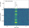 |
Fig. 1. Dynamic spectrum of FRB 20201020A, de-dispersed to a DM of 398.59 pc cm−3. The top panel shows the average calibrated pulse profile of the burst, and the bottom panel the intensity of the burst in time versus frequency. The data have been downsampled in frequency by a factor 8. |
The detection of bursts A17 and A53 from FRB 20180916B was originally reported in Pastor-Marazuela et al. (2021), where the observations and data reduction are explained.
2.1. Burst structure
After de-dispersing to the structure-maximising DM, the pulse profile shows five distinct components with no visible scattering. In order to better characterise the intensity variation with time, we fitted the pulse profile to a five-component Gaussian and give the result in Table 2. The ToAs are given with respect to the arrival of the first component, and the component width is defined as the full width at half maximum (FWHM). The resulting burst component widths at the DM of FRB 20201020A are very close to the intra-channel dispersive smearing of ∼250 μs at 1370 MHz given the Apertif time and frequency resolution (Petroff et al. 2022). Therefore, we can only set an upper limit on the scattering timescale of 0.25 ms. The total duration of the burst is 2.14(2) ms.
Properties of the five FRB 20201020A components.
The burst shows frequency-dependent intensity variations, which is a phenomenon expected from scintillation produced by propagation through the turbulent interstellar medium (ISM; see Sect. 4.2.2 from Lorimer & Kramer 2004, and references therein). In order to measure the decorrelation bandwidth of the fluctuations, ΔνFRB, we generated the auto-correlation function (ACF) of the burst averaged spectrum, defined as follows:
 (1)
(1)
where S(ν) is the burst-averaged, mean subtracted spectrum at frequency ν and Δν is the frequency lag. This is computed at the original frequency resolution. After removing the zero-lag value, we fitted the central peak of the ACF to a Lorentzian. The scintillation bandwidth is often defined as the half-width at half-maximum (HWHM) of the fitted Lorentzian (Cordes 1986), as shown in the top panel of Fig. A.1. The YMW16 (Yao et al. 2017) and NE2001 (Cordes & Lazio 2003) models give the distribution of free electrons in the Milky Way (MW), and can therefore be used to estimate the DM, scattering, and scintillation contribution from the Galaxy. The scintillation bandwidth of ΔνFRB = 11.4(2) MHz does not strongly deviate from the NE2001 model predictions at 1370 MHz, where ΔνNE2001 ∼ 16.0 MHz2. The YMW16 model predicts a similar MW scintillation bandwidth of ΔνYMW16 ∼ 10.4 MHz in the direction of the FRB. This model does not simulate the scattering or scintillation; instead it models DMs and then uses the empirical τ–DM relation observed in Galactic pulsars to determine the scattering. Nevertheless, it approaches ΔνNE2001 in the direction of the FRB, and coincidentally matches the observed decorrelation bandwidth of FRB 20201020A assuming 20% errors.
The ACF presents strong secondary peaks that appear quasi-periodic, especially the one with a ∼50 MHz frequency lag. This might indicate that the frequency structure is intrinsic to the FRB, instead of being due to scintillation in the MW. Such intrinsic structure has been noted in other high-luminosity radio emission mechanisms: the interpulses of the Crab pulsar consist of regularly spaced spectral bands (Hankins & Eilek 2007). To test this possibility, we studied the frequency evolution of the decorrelation bandwidth. If the fluctuations in the spectrum are produced by scintillation, the decorrelation bandwidth should roughly follow a power law with spectral index 4.0–4.4 (e.g., Cordes et al. 1985). We therefore divided the FRB spectrum into four different sub-bands of 75 MHz bandwidth each. We computed the ACF of each sub-band and fitted them to a Lorentzian. As detailed in the Appendix A and Fig. A.1, the decorrelation bandwidth of FRB 20201020A does not appear to follow the evolution expected from scintillation. However, the amount of frequency fluctuation per observing bandwidth is too small, and snapshots of scintillation frequency structure can appear quasi-periodic.
Scintillation could also be produced in the host galaxy, although it is unlikely that it would match the scintillation bandwidth expected from the MW. We cannot confidently rule out that the intensity fluctuations with frequency are an intrinsic property of the FRB. Importantly, their relative spacing of Δν/ν = 50/1400 = 0.04 is in reasonable agreement with the Δν/ν ≃ 0.06 proportional spacing found for the Crab interpulses in Hankins & Eilek (2007). Scintillation in the MW may yet be the most probable explanation, as the observed decorrelation bandwidth is close to the NE2001 prediction.
By eye, all burst components seem to cover a similar frequency extent. In order to thoroughly check whether the subcomponents exhibit a downward drift in frequency, we computed the 2D auto-correlation function of the burst, which we ultimately fitted to a 2D ellipse whose inclination gives a good estimate of the drift rate (Hessels et al. 2019). The resulting 2D ACF shown in Fig. B.1 shows an inclination angle consistent with zero, which means there is no subcomponent frequency drift, as expected from one-off FRBs.
2.2. Localisation
As the WSRT is an array in the east–west direction, it can localise any detected FRB to a narrow ellipse (cf. Connor et al. 2020). FRB 20201020A was detected in three adjacent CBs; CB29, CB35, and CB28. Following the localisation procedure as described in Oostrum (2020)3, we used the S/N of the burst in all synthesised beams (SBs) of all CBs where it was detected in order to get its 99% confidence region. We find the best position to be 13 h51 m25 s + 49°02′06″ in right ascension (RA) and declination (Dec) respectively. The localisation area is shown in Fig. 2, and it can be well described as a 3.9′×17.2″ ellipse with an angle of 103.9° in the north–east direction.
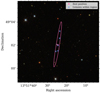 |
Fig. 2. Localisation region of FRB 20201020A. The best position is indicated by a pink cross, and the 99% confidence interval contour is represented by the pink ellipse. Galaxies from the NED database within the error region are marked as blue crosses. The background is a composite colour image from SDSS (Blanton 2017). |
The DM expected from the MW in the direction of the FRB is ∼22 pc cm−3 according to the YMW16 model and ∼29 pc cm−3 according to NE2001. By assuming a MW halo contribution to the DM of ∼50 pc cm−3 (Prochaska & Zheng 2019), we find an extragalactic DM of ∼325 pc cm−3, and use this to estimate a redshift upper limit4 of zmax ∼ 0.43 (Zhang 2018; Planck Collaboration VI 2020; Batten 2019).
We queried the NASA/IPAC extragalactic database (NED) to identify potential host galaxies of FRB 20201020A. We found five galaxies within the error region catalogued in the SDSS-IV MaNGA (Graham et al. 2018), which is based on the fourteenth data release of the Sloan Digital Sky Survey (SDSS-DR14; Abolfathi et al. 2018) and has a 95% magnitude completeness limit of 22.2 in the g filter5. None of the five galaxies have a measured redshift or morphological type. Any one of those five galaxies could therefore be the host of FRB 20201020A, and there could be galaxies below the magnitude completeness of SDSS-DR14. The galaxies are listed in Table C.1.
2.3. Polarisation and rotation measure
The detection of FRB 20201020A triggered a dump of the full-Stokes data on CB29, allowing us to measure the polarisation properties of FRB 20201020A. We carried out calibration observations within 36 h of the FRB detection. We pointed at the unpolarised source 3C147 and the linearly polarised source 3C286 to correct for the difference in gain amplitude between the x and y feeds and the leakage of Stokes V into Stokes U, respectively (cf. Connor et al. 2020). The polarisation properties of FRB 20201020A could provide important information about the nature of this source. For instance, in the case of a rotating neutron star (NS), one might expect changes in the polarisation position angle (PPA) following the rotating vector model (RVM; Radhakrishnan & Cooke 1969), as shown by about 50% of pulsars (e.g., Johnston et al. 2023).
Unfortunately, the polarisation calibration observations were corrupted by radio frequency interference (RFI) and their poor quality prevents robust PPA measurements. Nevertheless, an estimate of the rotation measure (RM) can still be computed although with large uncertainties by assuming a constant value of Stokes V with frequency. From the resulting Stokes Q and U parameters, we obtain the best RM by applying RM synthesis (Burn 1966; Brentjens & de Bruyn 2005), and we check the resulting RM by applying a linear least squares fit to the position angle (PA) as a function of wavelength squared. We find an RM of +110 ± 69 rad m−2, which is visualised in Fig. D.1.
2.4. Repetition rate
The localisation region of FRB 20201020A has been observed for 107.8 h with Apertif since the beginning of the survey in July 2019. This observing time includes follow up observations of both FRB 20201020A and FRB 20190303A (Fonseca et al. 2020). We therefore set a 95% upper limit on the repetition rate of ∼3.4 × 10⁻² h−1 above our completeness threshold of 1.7 Jy ms assuming a Poissonian repetition process. This upper limit is roughly one order of magnitude lower than the average repetition rates observed in FRB 20121102A and FRB 20180916B in observations carried with Apertif (∼0.29 h−1 and ∼0.36 h−1, respectively Oostrum 2020; Pastor-Marazuela et al. 2021), which therefore have an equivalent completeness threshold. However, we note this limit may be less constraining if the FRB has non-Poissonian repetition, as has been seen for other FRBs (Spitler et al. 2016; Oppermann et al. 2018; Gourdji et al. 2019; CHIME/FRB Collaboration 2020a; Hewitt et al. 2022).
3. Timing analysis
We applied several timing techniques in order to determine the presence of a periodicity in FRB 20201020A, and the FRB 20180916B bursts A17 and A53. Initially, we obtained the power spectra of each pulse profile – defined as the Leahy normalised (Leahy et al. 1983) absolute square of the fast Fourier transform (FFT) – in order to identify any potential peaks in the power spectrum of each burst.
Additionally, all three pulse profiles were fitted to multi-component Gaussians in order to determine the time of arrival (ToA) of each burst subcomponent. The ToAs as a function of component number were subsequently fitted to a linear function of the form
 (2)
(2)
where ti is the ith arrival time;  is the mean spacing between the subcomponents of each burst, equivalent to Psc; ni is the ith component number; and T0 is the first ToA. For the fit, we use a least squares minimisation technique weighted by the inverse of the errors on the ToAs in order to determine the mean subcomponent separation Psc and the goodness of fit. We performed these fits using the Python package lmfit6 (Newville et al. 2016). In our analysis, we used the reduced χ2 (rχ2) statistic, which takes into account the statistical error on the reported ToAs. We also applied the rχ2 statistic to CHIME FRBs 20210206A and 20210213A for comparison. Given the necessity of fitting a model to the tail of the distribution of the simulated statistics for FRB 20191221A in CHIME/FRB Collaboration (2022) and the high significance found, we do not compare the statistics of FRB 20191221A with FRB 20201020A in this work. Furthermore, we applied the statistic
  as described in CHIME/FRB Collaboration (2022) in order to have a direct comparison between our sample and the FRBs presented there. The
  statistic is obtained by finding the component number combination n that maximises the log-likelihood ratio
  between two models, after maximising all model parameters. The first model is the null hypothesis that the ToAs follow a Gaussian distribution, and the second is the alternate hypothesis that the ToAs follow the linear function given by Eq. (2), where we have
![Mathematical equation: $$ \begin{aligned} \hat{L}[n] = \frac{1}{2} \log \left( \sum _i \dfrac{(t_i - \bar{t_i})}{r_i}\right), \end{aligned} $$](/articles/aa/full_html/2023/10/aa43339-22/aa43339-22-eq7.gif) (3)
(3)
with ri the difference between the measured and the fitted ti, and
![Mathematical equation: $$ \begin{aligned} \hat{S}[n] = \max _n \left( \hat{L}[n] \right). \end{aligned} $$](/articles/aa/full_html/2023/10/aa43339-22/aa43339-22-eq8.gif) (4)
(4)
The rχ2 statistic is more adapted to the ToAs and errors obtained through our pulse profile fitting routine than the  statistic, given that the latter does not take the errors into account, and the rχ2 statistic does not substantially alter the periodicity significance of the CHIME FRBs 20210206A and 20210213A. We therefore find it to be more robust when computing periodicity significances.
Lastly, we computed the significance of the potential periodicities by simulating the ToAs of 105 bursts. This consists in generating time intervals di = (ti − ti − 1) drawn from different distributions. Following the procedure presented in CHIME/FRB Collaboration (2022), we first assume a rectangular probability distribution which is uniform between two values:
 (5)
(5)
where 0 ≤ η≤ is an exclusion parameter (originally referred to as χ in CHIME/FRB Collaboration (2022), renamed to avoid confusion with rχ2), below which two separate components would be detected as one. This distribution is normalised and centred at the mean subcomponent spacing. We use Π to represent this rectangular function. We adopt η = 0.2 following the analysis from the CHIME FRBs. We label the significance using the rχ2 statistic σχ2, and  the one using the
  statistic.
We also simulate the time intervals from a shifted Poissonian distribution as a comparison, where we have
 (6)
(6)
and x is a random variable drawn from a uniform distribution between 0 and 1. This gives a distribution of time intervals with average  and minimum η. We note that when η = 0,
  , which gives the exponentially distributed inter-arrival times of a Poissonian distribution. However, this distribution would produce inter-arrival times that are shorter than the width of the subcomponents, which justifies a choice of η > 0. We use P to represent this shifted Poissonian distribution.
We use these rectangular and shifted Poissonian wait-time distributions as null hypotheses because empirical wait-time distributions are not yet available. Determining the underlying wait-time distribution is hampered by significant selection effects, for both one-off and repeating FRBs (e.g., Gardenier et al. 2019, 2021). However, as surveys produce ever larger homogeneous samples (e.g., Pastor-Marazuela et al., in prep., for Apertif), we expect such empirical distributions to become available in the near future.
Figure 3 contains the relevant plots resulting from the timing analysis assuming a uniform probability distribution, while Table 3 gives the resulting rχ2 and  statistics assuming η = 0.2, as well as the significance of the FRB periodicities. Table E.1 gives the obtained significances and percentiles under different null hypotheses, subcomponent spacing distributions, and η values.
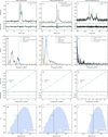 |
Fig. 3. Timing analysis of FRB 20201020A (left column), A17 (central column), and A53 (right column). The top of panels (a), (e), and (i) shows the pulse profile of each burst (black) and the fitted multi-component Gaussians in green for FRB 20201020A and A53; for A17 the bright components are shown in blue and the dim components in yellow. The bottom of panels (a), (e), and (i) shows the residuals of the multi-component Gaussian fit of each pulse profile. Panels (b), (f), and (j) show the power spectra of each pulse profile in black. In (b), the vertical dashed line indicates the average separation of the FRB 20201020A components, while the blue line shows the Gaussian fit to the 2.4 kHz component. In (f), the blue and yellow lines show respectively the power spectra of the bright and dim components. Panels (c), (g), and (k) show the ToAs of all subcomponents as a function of component number. In most cases, the error on the ToAs is smaller than the marker size. The dashed green lines in (c), (g), and (k) are linear fits to the ToAs, and the lower panels show their residuals normalised by the mean subcomponent separation Psc. Panels (d), (h), and (l) show histograms of the simulated rχ2 statistic using a shifted Poissonian subcomponent spacing distribution with η = 0.2 to compute the significance of the periodicity. The vertical lines correspond to the rχ2 of the linear fit to the data. The significance is indicated as blue text. |
Statistical significance of the FRB periodicities.
3.1. FRB 20201020A
To get the mean subcomponent separation Psc, we fitted the ToAs given in Table 2 as a function of component number n = (0, 1, 2, 3, 4). We get Psc = 0.411(6) ms, which we assume to be the period whose significance we want to examine.
The power spectrum of the FRB shows a peak at the frequency corresponding to the mean subcomponent separation, fsc = 2435 Hz. However, it also displays a peak with a higher amplitude at half the frequency corresponding to Psc. We argue that this peak is more prominent because of the higher amplitude of components 0, 2, and 4, which are spaced by twice the Psc. Additionally, the ToA of component 1 is delayed with respect to the others, as can be seen in panel c of Fig. 3, therefore lowering the power of the peak at 2435 Hz. Red noise could also play a factor in increasing the peak amplitude. We therefore consider 2435 Hz to be the fundamental frequency, and interpret the 1200 Hz peak as a subharmonic dominated by the spacing of the two brightest components, n = 0, 2.
By using the rχ2 as the reference statistic, applying it to both the data and the simulations, and drawing the time intervals from a rectangular distribution (Eq. (5)), we obtain a significance of σχ2, Π = 2.50σ. Drawing time intervals from the shifted Poissonian distribution in Eq. (6) gives in turn a significance of σχ2, P = 2.60σ for η = 0 (purely Poissonian), and σχ2, P = 2.40σ for η = 0.2. Hereafter we report the significance from a shifted Poissonian with η = 0.2 for robustness. The different steps of the analysis are plotted in panels a–d of Fig. 3. While σχ2 and  are not significant enough for a conclusive periodicity detection, this FRB is visually analogous to the CHIME FRBs 20210206A and 20210213A. This suggests that these three bursts belong to the same morphological class of FRBs, which present quasi-periodic components in time, with all subcomponents showing a similar frequency extent.
For comparison against pulsar component periodicity studies it is useful to also determine the quality factor Q. From the width Δf of the main component in the power spectrum, this factor quantifies how strictly periodic the burst structure is by means of the frequency stability Q = fsc/Δf (Boriakoff 1976). Higher Q values signify more stable features. We follow the approach from Strohmayer et al. (1992), fitting a Gaussian to the power spectrum feature, and taking the width of σ as Δf. We find σ = 0.17 kHz (Fig. 3b) and hence Q = 2.4/0.17 ∼ 14 for FRB 20201020A.
3.2. FRB 20180916B bursts
In 2020, we carried out a long observing campaign of FRB 20180916B with Apertif, and 54 detections were presented in Pastor-Marazuela et al. (2021). Several of those bursts display complex spectro-temporal morphologies, with at least 12 bursts presenting three or more temporal components. While most of those multi-component bursts have either an excessively low subcomponent number, S/N, or subcomponent spacing to run a detailed timing analysis, two of the bursts (A17 and A53) have favourable properties to run this analysis, as detailed below.
Figure 4 shows the spacing distribution between the subcomponents of R3 bursts from Pastor-Marazuela et al. (2021) with two or more components. In addition to the timing analyses detailed above, we compute the periodicity significance of A17 and A53 by simulating time intervals from the subcomponent separation distribution observed in other multi-component bursts from FRB 20180916B. We get the distribution by fitting the observed subcomponent separations in Fig. 4 to a lognormal distribution:
 (7)
(7)
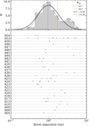 |
Fig. 4. Subcomponent separation of FRB 20180916B multi-component bursts presented in Pastor-Marazuela et al. (2021). The top panel shows a histogram of the burst separation between discernible subcomponents in multi-component bursts. The mean A17 and A53 separations are shown as vertical dashed blue and yellow lines, respectively. The fit to a single lognormal and a double lognormal distribution are shown as solid and dotted black lines, respectively. The bottom panel shows the burst separations in each burst of the sample. |
where A is the amplitude, m the mean, and σ the standard deviation. We use  as errors for the fit, with N the number of subcomponent separations per bin. The resulting parameters of the fit are m = 0.98 ± 0.06 ms and σ = 0.64 ± 0.06. We label σln the significance of the periodicity obtained from assuming this separation distribution. Although the separation distribution might appear bimodal at first glance, and a fit to a double lognormal distribution results in a lower χ2, a lower Akaike information criterion (AIC), and a lower Bayesian information criterion (BIC), we use the simpler, single lognormal distribution given the limited size of our sample. The waiting time between consecutive pulses in active repeaters has been observed to follow bimodal lognormal distributions by several authors, for example in FRB 20121102A (Aggarwal et al. 2021; Hewitt et al. 2022), FRB 20200120E (Nimmo et al. 2023), and FRB 20201124A (Niu et al. 2022). However, analyses of the subcomponent separations in large burst samples are scarce. Niu et al. (2022) performed a timing analysis on 53 bursts with complex morphologies from FRB 20201124A, and report the quasi-periods observed in their subcomponents. The quasi-period distribution can be fitted to a lognormal distribution with m = 6.0 ± 0.4 ms and σ = 0.52 ± 0.07 (from the values reported in their Table 6 and visualised in their Fig. 8). As repeating FRB timescales appear to follow lognormal distributions on millisecond and decasecond timescales, it is reasonable to assume this distribution for subcomponent spacings as well.
3.2.1. FRB 20180916B A17
The burst A17 from Pastor-Marazuela et al. (2021) has the highest detection S/N of the sample. Its pulse profile can be well fitted by a five component Gaussian, with the second and third components being much brighter than the others. Its power spectrum shows a large peak at ∼1000 Hz. As the separation between the second and third components is ∼1 ms, we tested whether the power spectrum was dominated by these two bright subcomponents instead of arising from an intrinsic periodicity. To do so, we created fake pulse profiles of the ‘bright’ and ‘dim’ components. The pulse profile of the bright components was created by subtracting the Gaussian fit of the first, fourth, and fifth components from the data, and the pulse profile of the dim components by subtracting the fit of the second and third components from the data. Next we generated power spectra of the ‘bright’ and ‘dim’ pulse profiles, both over-plotted in panel (f) of Fig. 3. As the power spectrum of the bright components largely overlaps with the power spectrum of the original pulse profile, we conclude that the peak in the power spectrum is dominated by the two brightest components.
We further fitted the ToAs to a linear function and compared the resulting rχ2 and  statistics to simulations, and find disparate values with σχ2, Π = 1.75σ and
  . When simulating the subcomponent separation from the shifted Poissonian distribution in Eq. (6) with η = 0.2, we get σχ2, P = 1.79σ, and from the lognormal distribution shown in Fig. 4, we find σχ2, ln = 1.87σ. Given this discrepancy, we cannot confirm the presence of a periodicity in A17. The steps of the timing analysis are plotted in panels e to h of Fig. 3.
3.2.2. FRB 20180916B A53
A53 is the widest FRB 20180916B burst, containing the highest number of components (≥11) presented in Pastor-Marazuela et al. (2021), making it a good candidate for periodicity analysis. Although the ToAs plotted as a function of component number show irregularities in the spacing between bursts, we still carried out the fit to a linear function and the significance computation by associating the larger ‘gaps’ to missing components, resulting in a component number vector n = (0, 1, 2, 4, 5, 6, 7, 10, 12, 13, 14, 15). We find  , σχ2, Π = 1.94σ, σχ2, P = 2.29, and σχ2, ln = 2.35σ.
Although the results from the previous analysis indicate that the structure of burst A53 is unlikely to be periodic, we carried out a more detailed analysis of the light curve, power spectrum, and ACF in order to disentangle any interesting features in this complex burst. First, we studied the power spectrum; at first glance, it appears to be consistent with a power law, as can be seen in Fig. 5d. Such a power spectrum is observed in different astrophysical sources, such as AGN, X-ray binaries, and magnetars (e.g., Vaughan et al. 2003; Huppenkothen et al. 2013) and is known as ‘red noise’. We therefore fitted the power spectrum to the following power-law function:
 (8)
(8)
with K the amplitude, α the power law slope, and C a constant representing the white noise component. To perform the fit, we applied an equivalent of a Bayesian maximum likelihood estimator with the Stingray spectral timing library (Huppenkothen et al. 2019). We sampled the posterior probability distribution of the parameters through a Markov chain Monte Carlo (MCMC) algorithm to obtain their actual distribution. We found α = 1.1(2). In order to search for any potential narrow features, we followed Nimmo et al. (2021) and Huppenkothen et al. (2014) and computed the residuals R(ν) of the power spectrum P(ν) defined as:
 (9)
(9)
where M(ν) is the value of the best-fit power law at frequency ν. We wanted to test whether the largest peak in the power spectrum, max(R(ν)), was consistent with noise. To do so, we simulated 100 power spectra by drawing power-law parameters from the MCMC sample. We multiplied each frequency bin of the MCMC-derived power laws by random noise simulated from a χ2 distribution with two degrees of freedom, and divided by two (Huppenkothen et al. 2014). We then fitted the simulated power spectra to a power-law function. We generated the simulated residuals Rsim(ν) using Eq. (9), and found max(Rsim(ν)), which we compare to max(R(ν)). Using this method, we found no statistical outliers in the A53 power spectrum.
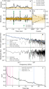 |
Fig. 5. Timing analysis of burst A53 from FRB 20180916B. Panel (a) shows the pulse profile of A53 as grey dots at 82 μs time resolution, and the smoothed profile as a black solid line. The yellow dots and solid line show the same for the off-burst signal. Panel (b) shows the residuals of the on- and off-burst signal as black and yellow lines, respectively. Green diamonds and dots show respectively the 5σ and 3σ outliers of the on-burst residuals. Panel (c) shows the distribution of the on-burst residuals in black and off-burst residuals in yellow. The yellow shaded regions, from dark to light, indicate the 1σ, 2σ, and 3σ contours of the off-pulse distribution fitted to a Gaussian. Panel (d) shows the power spectrum of A53 in black fitted to a power-law function shown in blue. The green dashed and yellow dotted lines mark the position of the mean component separation and the maximum of the residuals, respectively. Panel (e) shows the power spectrum residuals R(ν). Panel (f) presents the ACF of the light curve of A53 as a solid black line. The pink vertical lines indicate the separation between consecutive components, the green line the separation between the two brightest components, and the blue line the separation between the first and third brightest components. |
The pulse profile of A53 shows several spikes only one or two time bins wide. To check whether these narrow features have a physical origin or if they are consistent with amplitude-modulated noise (Rickett 1975; Cordes 1976), we followed the method described in Nimmo et al. (2021). We selected a 40 ms window that encompasses the whole signal from the burst, and created a model of the burst envelope by convolving the signal with a Blackman window of length 15. We obtained the residuals by subtracting the smoothed envelope from the burst signal, and we did the same with an off-burst region to obtain the distribution of the noise fluctuations. We observe that the residuals from the burst signal, when compared to the noise residuals, present two sets of outliers at a 5σ level, and two additional outliers at a 3σ level (we consider a set of outliers when they are spaced by a single time bin). This demonstrates that the narrow spikes have a physical origin, and are not the product of amplitude-modulated noise. The steps of this analysis are presented in panels a–c of Fig. 5. We determined the width of the two narrowest and brightest components by fitting them to a Gaussian together with the other components of the burst, as shown in Fig. 3i. Their full widths at half maximum (FWHMs) are respectively 220 μs and 175 μs.
We also show the ACF of the pulse profile in Fig. 5f. Although the ACF presents several secondary peaks, these can be explained by the separation between subcomponents, including consecutive ones and the brightest ones. These peaks are therefore not due to the presence of a periodicity.
4. Discussion
After determining the periodicity significance of FRB 20201020A, A17, A53, and the CHIME FRBs 20210206A and 20210213A, we note that the measured significance of the burst (quasi-)periodicities is highly dependent on the null hypotheses and the assumed subcomponent spacing of the aperiodic simulations, as shown in Table E.1. As noted by Niu et al. (2022), when analysing the temporal structure of FRB 20201124A bursts, it is necessary to be cautious about quasi-periodicities with significances below ∼4σ.
In the following section, we consider which mechanism can best explain the quasi-periodicity in FRB 20201020A: the rotation of an underlying submillisecond pulsar (Sect. 4.1), the final orbits of a compact object merger (Sect. 4.2), crustal oscillations after an X-ray burst (Sect. 4.3), or equidistant emitting regions on a rotating NS (Sect. 4.4). We also comment on whether or not these FRBs represent a new morphological type.
4.1. Submillisecond pulsar
One of the potential origins of the periodic structures in FRB 20201020A and the CHIME FRBs 20210206A and 20210213A discussed in CHIME/FRB Collaboration (2022) is the rotation of a NS with beamed emission, analogous to spin-driven radio pulsars. While the period range observed in the aforementioned FRBs is compatible with Galactic pulsars, the quasi-period of FRB 20201020A, Psc = 0.411 ms, is in the submillisecond regime.
A spin rate of such magnitude is interesting because it could provide the energy required for the highly luminous radio emission seen in FRBs in general. For a rotation-powered NS, the spin rate ν and surface magnetic field strength Bsurf determine the potential of the region that accelerates the particles that generate the radio bursts. For example, giant pulses are only common in those pulsars with the highest known values of ν3Bsurf, interpreted as the magnetic field strength at the light cylinder BLC (where BLC > 2.5 × 10⁵ G, Johnston & Romani 2004; Knight 2006). The spin frequency could therefore potentially power such luminous emission.
The next question, then, is for how long this emission can last. The same constituents that combine to provide the high power budget also cause rapid NS spin down. Such a high-powered system cannot therefore be long-lived, requiring a higher birth rate of these systems in the Universe to account for the observed FRB population (see e.g., Gardenier & van Leeuwen 2021). Creating an FRB may well require a much higher BLC field than a pulsar; a very young but otherwise normal NS with P = 0.411 ms and Bsurf = 1012 G shows a BLC field that is more than 1000 times higher than mentioned above for a little over 100 yr.
The FRB 20201020A quasi-period is shorter than that of the fastest spinning pulsar confirmed so far, with ∼1.4 ms (Hessels et al. 2006), and would be the smallest known NS spin period. The maximum rotation rate an NS can achieve can set important constraints on the NS equation of state (EoS; e.g., Shapiro et al. 1983). This maximum rotation rate is given by the mass-shedding frequency limit, above which matter from the outer layers of the NS is no longer gravitationally bound and is thus ejected. Haensel et al. (2009) establish an empirical formula for the mass-shedding frequency fmax given by the mass and radius of the NS, with C ∼ 1 kHz,
 (10)
(10)
Figure 6 shows a mass–radius diagram based on Demorest et al. (2010), including typical EoSs, the physical limits set by causality, finite pressure, and general relativity (GR; Lattimer 2012), and observational constraints given by the two most massive known NSs (Cromartie et al. 2020; Fonseca et al. 2021; Demorest et al. 2010) and the fastest spinning NS at 716 Hz (Hessels et al. 2006). We next plot the mass–radius relation using Eq. (10), assuming the mass-shedding frequency to be given by FRB 20201020A, fmax = 1/0.411 ms ∼ 2435 Hz. As no EoSs remain in the white region of the diagram, we conclude that the quasi-period of FRB 20201020A is incompatible with being due to the rotation of a NS using typical EoSs. If the three FRBs are originated by the same type of progenitor – given the similar morphological properties of FRB 20201020A and CHIME/FRB FRBs FRB 20210213A and FRB 20210206A –, the periodicity of the burst components is unlikely to be due to the rotation of a NS.
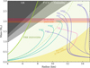 |
Fig. 6. Neutron star mass–radius diagram. The solid lines represent the mass–radius relationship of typical EoSs. The grey shaded regions are forbidden by general relativity, finite pressure (P < inf), and causality. The yellow shaded region is forbidden by the rotation of the fastest spinning pulsar J1748−2446ad (Hessels et al. 2006). The red shaded region shows the mass of J0740+6620 (Cromartie et al. 2020; Fonseca et al. 2021) and the orange region the mass of J1614-2230 (Demorest et al. 2010), the two heaviest known NSs. Valid EoSs need to cross those regions. The green line and green shaded region would be forbidden if the quasi-period of FRB 20201020A were produced by the rotation of a NS at 2435 Hz, and the region to the right of the dashed green line would be forbidden if the rotation was at 1205 Hz. |
4.2. Compact object merger
Merging compact objects have been hypothesised to produce FRBs through magnetic interaction between the two bodies in the system, including binary NS systems (BNS, Piro 2012; Lyutikov 2013; Totani 2013; Wang et al. 2016; Hansen & Lyutikov 2001), black hole–neutron star systems (BHNS; McWilliams & Levin 2011; Mingarelli et al. 2015; D’Orazio et al. 2016), and white dwarfs (WDs) with either a NS or a black hole (Liu 2018; Li et al. 2018). The presence of multiple peaks in the FRB pulse profile could be explained by a magnetic outburst extending through successive orbits of the binary system, and therefore the subcomponent frequency should match half the gravitational wave (GW) frequency if one object in the system produces bursts, or the GW frequency if both of them do. The maximal GW frequency is attained when the binary reaches the mass-shedding limit for an NS (Radice et al. 2020). This frequency is given by the EoS of the merging NS, which is expected to be between 400 and 2000 Hz (Bejger et al. 2005; Dietrich et al. 2021; Hanna et al. 2009).
The frequency seen in the components of FRB 20201020A of 2435 Hz is above the typical limits and can only be explained by a very soft EoS. Such a frequency could only be produced in the final moments of the inspiral, immediately before the merger. At this stage, the frequency derivative would be very high, which translates to a perceptibly decreasing spacing between burst subcomponents. As the separation remains constant within the burst, we can rule out this scenario for FRB 20201020A. A more detailed justification is given in Appendix F. The quasi-period of FRB 20210206A is also challenging to explain within this model (CHIME/FRB Collaboration 2022). As only a small fraction of the known FRBs show regularly spaced components, we argue that these belong to the same class of progenitor and hence disfavour compact object merger models as the progenitors of FRBs with this type of morphology.
4.3. Crustal oscillations
If FRBs are a result of short X-ray bursts from a magnetar, the quasi-periodicity we observe could be explained through crustal oscillations of the NS we describe above. These oscillations would result from the same X-ray burst that also caused the FRB (Wadiasingh & Chirenti 2020). The subcomponents of FRB 20201020A suggest an oscillation frequency of ∼2400 Hz. Wadiasingh & Chirenti (2020) examine whether or not FRB subpulses could be the result of torsional crustal oscillations during a short X-ray burst. If so, their simulations show that the fundamental eigenmodes with low multipole number (corresponding to frequencies between 20–40 Hz) would be more prevalent than the higher frequencies that we observe. We conclude that the difference in frequency is too large. The quality factor Q = 14 that we find in Sect. 3.1 is also significantly lower than the Q > 103 expected for NS oscillations (Cordes et al. 1990). We therefore disfavour crustal oscillations as the source of the periodicity.
4.4. Ordered emission regions on a rotating magnetar
The burst morphology and timescales of FRB 20201020A are very similar to two types of quasi-periodic behaviour seen in regular pulsars: subpulses and microstructure. Below we discuss scenarios where the FRB is produced in a similar manner, but on a magnetar instead of a purely rotation-powered pulsar.
4.4.1. The analogue of pulsar subpulses
Like the components in FRB 20201020A, the individual pulses of rotation-powered pulsars are usually composed of one or more subpulses. Subpulse widths lie in the range of 1° −10° in spin longitude (Table 16.1 in Lyne & Graham-Smith 2012), thus broadly spanning 0.3 − 140 ms for pulsars with spin periods of 0.1 − 5 s. This qualitatively fits the individual component widths of observed FRB structures.
For a substantial fraction of these pulsars (mostly those with longer periods), the position or intensity of these subpulses changes in an organised fashion from one spin period to another (Weltevrede et al. 2007; Basu et al. 2019). According to the most widely accepted theory of drifting subpulses, these latter are interpreted as emission from distinct plasma columns originating in a rotating carousel of discharges within the polar gap (Ruderman & Sutherland 1975). As the NS spins, these ordered, regularly spaced emission regions (‘sparks’) produce quasi-periodic bursts in our line of sight. In this case, the burst morphology directly reflects the spatial substructure of the distinct emission regions. Given the similarity in appearance, we hypothesise here that a magnetar produces the components in FRB 20201020A in the same way that a pulsar produces subpulses.
This carousel rotation causes subpulses to appear at progressively changing longitudes7. Every period may contain one or a few individual subpulses roughly equidistant from each other. These regular subpulses cause a stable second periodicity on top of the primary rotational periodicity. In the most regular cases, the resulting drifting subcomponents show a relatively periodic behaviour; in PSR B0809+74 (van Leeuwen et al. 2003), the spark rotation and spacing were recognised early on to be stable at a 0.4% level over several days (Unwin et al. 1978). Overall, the spark regularity is sufficient to produce the quasi-periodicity we observe here.
The residuals in the timing fit of FRB 20201020A (Sect. 3.1) also have an analogue in pulsar subpulses. There, the deviation from strict periodicity within a single pulsar rotation is well-documented for some of the sources with more stable drift and is well described by the curvature of the line-of-sight path through the emission cone (Edwards & Stappers 2002; van Leeuwen et al. 2002). At least for some sources, the drifting rate can be measured with good precision (indicating prominent periodic modulation), and it has been shown that it can slowly vary with time (Rankin & Suleymanova 2006) and jitter on small timescales (van Leeuwen & Timokhin 2012), and can change rapidly during a mode switch (Janagal et al. 2022). Several drift periodicities can even be present at the same time at different spin longitudes (bi-drifting; Szary et al. 2020).
Pulsar subpulses are not only similar to the components in FRB 20201020A, the CHIME FRBs 20210206A and 20210213A, and A17 with respect to their regular spacing; the number of subcomponents also agrees. A significant number of pulsars, such as B0329+54 (Mitra et al. 2007), B1237+25 (Srostlik & Rankin 2005), and B1857−26 (Mitra & Rankin 2008), show both a similarly high number of distinct subpulses and quasi-periodically spaced single pulse profiles.
One concern in this analogy might be the timescale of the ‘on-mode’ for FRBs. If the FRBs we discuss here come from a single NS rotation, the absence of fainter bursts nearby means the subpulse pattern flares for one period and then turns off. This may seem problematic. Nevertheless, for pulsars that display nulling, or different modes of emission, the spark pattern is known to establish itself very quickly, at the timescale of less than a spin period (Bartel et al. 1982). Furthermore, pulsars such as J0139+3336 (a 1.25 s pulsar that emits a single pulse only once every ∼5 min; Michilli et al. 2020) and the generally even less active rotating radio transients (RRATs; McLaughlin et al. 2006) show that a population of NSs exists that produce bright but sporadic emission. Overall, while the amount of information available for FRBs is limited, their behaviour falls within the (admittedly broad) range of features exhibited by subpulse drift.
4.4.2. The analogue of pulsar/magnetar microstructure
In pulsars, the individual subpulses mentioned in the previous sections themselves often contain yet another level of μs–ms substructure (Kramer et al. 2002). Often narrow micropulses are observed in groups of several spikes riding on top of an amorphous base pulse; although deep modulation down to zero intensity has also been observed (Cordes et al. 1990). This so-called microstructure is about three orders of magnitude narrower (∼μs) than the enveloping subpulses (∼ms), and the spacing between spikes is quasi-periodic. For the well-studied pulsar PSR B2016+28, for example, Strohmayer et al. (1992) find a Q value (Sect. 3.1) of 5.7. In a set of four more pulsars, Cordes et al. (1990, their Table 2) also find Q values of ∼5. The stability we find for FRB 20201020A, Q = 14, is somewhat higher than in these pulsars. However, for other models (e.g., Sect. 4.3), there were much larger discrepancies for Q. We therefore find the FRB Q value agrees with those seen in pulsar micropulses.
A linear relation between the periodicity of the microstructure and the pulsar spin period has been established; first for pulsar spanning the period range 0.15 − 3.7 s (Mitra et al. 2015), and next extended to millisecond pulsars (De et al. 2016). Recent observations of the 5.5-second magnetar XTE J1810−197 also generally agree with the linear microstructure–period relationship (Maan et al. 2019). The relation strongly suggests a physical origin, but the exact mechanisms for the microstructure remains unclear. There are two main theories: a geometrical one, based on distinct tubes of emitting plasma; and a temporal one, based on modulation of the radio emission (see the discussion in Mitra et al. 2015).
If we hypothesise that variations in FRB emission follow from processes similar to microstructure, then in the geometrical interpretation the FRB components are created when distinct spatial structures in the magnetosphere of a rotating, FRB-emitting NS pass, in turn, through our line of sight. In the temporal interpretation, the entire FRB envelope is produced by a single, wider beam from a rotating NS. Temporal modulations in this beam then produce the substructure variations.
Even if the FRB subcomponent resemblance to pulsar microstructure does not immediately allow for their exact physical interpretation, we can still apply the empirical periodicity–period relation from Mitra et al. (2015) to these FRBs. Their observed subcomponent periodicities lead to tentative NS spin periods of between 0.3 and 10 s.
In microstructure, an increase of pulsar period is met by a linear increase in the component periodicity, as we discuss immediately above. A similar relation with the spin period is seen for the micropulse widths (Cordes 1979; Kramer et al. 2002). If we again consider the different components in FRB 20201020A as microstructures, we can also apply this relation. In FRB 20201020A, the average intrinsic component width (i.e. after accounting for the inter-channel dispersion smearing and the finite sampling time), defined as the FWHM, is 250 ± 30 μs, suggesting a tentative NS spin period in the range of 0.3–0.6 s. Given their required intrinsic brightness, FRBs might actually be more closely related to the giant micropulses as seen in the Vela pulsar (Johnston et al. 2001). On average, those have even narrower widths (Kramer et al. 2002). However, the bright single pulses from magnetar XTE J1810−197 could be giant micropulses; and still these agree with the standard linear relationship between the normal micropulse width and spin period (Maan et al. 2019). There therefore appears to be some scatter in these relations. We conclude that if FRB 20201020A consists of such giant micropulses, the tentative NS spin period may increase, and fall on the higher side of the above estimated period range.
One characteristic feature of microstructure is that linear and circular components of emission closely follow quasi-periodic total intensity modulation. This is also true for FRB 20210206A, the only FRB presented in CHIME/FRB Collaboration (2022) with a measurable polarised signal. Unfortunately, as mentioned in Sect. 2.3, we were not able to obtain a robust Stokes parameter calibration, which would have been useful for comparison with typical pulsar microstructure features.
4.4.3. The magnetar connection
The microstructure that was previously known only in pulsars has recently also been observed in radio emission from magnetars, especially in the radio-loud magnetar XTE J1810-197. This suggests a further expansion into FRBs is worth considering. The 2018 outburst of XTE J1810-197 led to high-resolution detections and studies at different epochs and radio frequencies (Levin et al. 2019; Maan et al. 2019; Caleb et al. 2021). The magnetar exhibits very bright, narrow pulses; and for discussions on the classification of these, we refer to Maan et al. (2019) and Caleb et al. (2021). The source also exhibits multi-component single pulses that show quasi-periodicity is the separation between different components. If we assume FRBs originate from magnetars, it is possible that the quasi-periodicity that is seen in the sample presented in this paper can be tied to a similar underlying emission mechanism on a different energy scale. Much of the available energy budget is determined by the period and magnetic field. The spin-period range we find covers the periods of the known magnetars. Magnetars with a relatively short period of about ≳2 s plus a strong surface magnetic field of > 1014 G would produce a larger vacuum electric field (due to the rotating magnetic field) than normal, slower magnetars. While part of this vacuum field will be shielded out, the fraction that remains present in the plasma-starved regions is responsible for the particle acceleration. Short-period, high-field magnetars could therefore conceivably generate stronger acceleration and larger Lorentz factors such as those required for FRB luminosities. It would be interesting to compare the FRB luminosity of sources with different supposed spin periods within this model.
4.5. Morphological type
Based on the first CHIME/FRB catalogue, Pleunis et al. (2021) identified four FRB types based on their morphology. These classes are simple broadband, simple narrowband, temporally complex and downward drifting. Downward drifting bursts are commonly associated with repeating FRBs (Hessels et al. 2019), and A17 and A53 are unequivocal examples of this morphological type. Bursts classified as temporally complex are those presenting more than one component peaking at similar frequencies, but with no constraint on the separation between components. This class makes up for 5% of the FRBs presented in the CHIME/FRB catalogue, but ≲0.5% of the FRBs show five or more components.
With the detection of FRB 20191221A, FRB 20210206A, and FRB 20210213A, CHIME/FRB Collaboration (2022) propose the existence of a new group of FRBs with periodic pulse profiles. FRB 20201020A is the first source detected by an instrument other than CHIME/FRB showing a quasi-periodic pulse profile, thus adding a new member to this nascent FRB morphological type. Whether all burst profile classes can be formed by a single progenitor type, or whether these signify physically distinct progenitors is an ongoing matter of debate (cf. Petroff et al. 2022).
All three FRBs, namely FRB 20201020A and the CHIME FRBs 20210206A and 20210213A, have six components or fewer, and none of these FRBs reach a 3σ significance for the periodicity. This could be explained by the structure of the magnetosphere of magnetars formed by roughly equally spaced emission regions. The higher number of components in FRB 20191221A might reduce the effect of jitter in each single component and thus increase the significance of the periodicity. Alternatively, given its longer period, envelope duration, and higher periodicity significance, the CHIME FRB 20191221A could have been produced by a magnetar outburst lasting several rotations or a single burst comprising crustal oscillations.
Considering the scarcity of FRBs with a regular separation between components, the detection of FRB 20201020A is remarkable given that the number of events detected with Apertif is a few orders of magnitude lower than CHIME/FRB. This suggests that a larger fraction of FRBs with quasi-periodic components might be visible at higher frequencies. Certain astrophysical and instrumental effects could play a role at blurring together multi-component bursts at lower frequencies. This includes interstellar scattering, which evolves as τ ∼ ν−4, as well as intra-channel dispersive smearing, which scales as ν−3, and finite sampling of existing instruments that prevent detection of components narrower than the sampling interval. Searches of multi-component FRBs with a regular spacing might therefore be more successful at higher frequencies.
The bursts A17 and A53 from FRB 20180916B discussed in this work, although similar to FRB 20201020A at first glance, do not show conclusive evidence for periodicity in their subcomponents. This, added to the downward drift in frequency of the subcomponents common in bursts from repeating FRBs, differs from FRB 20201020A and the CHIME/FRBs FRB 20191221A, FRB 20210206A, and FRB 20210213A. This might suggest the presence of a different emission process between the bursts from repeating FRBs and the FRBs with quasi-periodic components, or an additional mechanism modulating the bursts.
5. Conclusions
In this paper, we present a new fast radio burst detected with Apertif, FRB 20201020A. This FRB shows a quasi-periodic structure analogous to the three FRBs presented in CHIME/FRB Collaboration (2022). However, the average spacing between its five components is ∼0.411 ms, in the submillisecond regime. We performed a timing analysis of the FRB, and conclude that the periodicity has a marginal significance of ∼2.4σ, which is comparable to the significance of the CHIME FRBs 20210206A and 20210213A. Given the scarcity of FRBs with quasi-periodic structure detected so far, these particular FRBs were likely produced via the same mechanism, and we postulate that they constitute a new FRB morphological type.
Additionally, we performed a timing analysis of bursts A17 and A53 from Pastor-Marazuela et al. (2021), the bursts with the highest number of visible subcomponents, but find no conclusive evidence of periodicity in these bursts. In A53, a burst with 11 or more components, we find an average subcomponent spacing of ∼1.7 ms. For the five-component burst A17, the average subcomponent separation is ∼1 ms. These timescales are of the same order of magnitude as the subcomponent separation in FRB 20201020A.
We discussed several interpretations of the quasi-periodicity, and we rule out the submillisecond pulsar and the binary compact object merger scenarios as potential progenitors to FRB 20201020A. However, its morphology is comparable to pulsar subpulses and pulsar microstructure, and similar structures have been observed in single pulses from radio-loud magnetars. We therefore conclude that the structure in the magnetosphere of a magnetar could be at play in producing bursts such as FRB 20201020A and the CHIME FRBs 20210206A and 20210213A. On the other hand, given the high significance of the period detected in FRB 20191221A, as well as the higher burst separation of ∼200 ms, the structure seen in this CHIME/FRB burst could have been produced by a magnetar outburst lasting several NS rotations.
Values estimated at 1370 MHz with the pygedm package: https://pygedm.readthedocs.io/en/latest/
Localisation code can be found here: https://loostrum.github.io/arts_localisation/
The redshift upper limit was computed with the fruitbat package assuming a Planck18 cosmology and the Zhang (2018) method: https://fruitbat.readthedocs.io/en/latest/
See SDSS-DR14 information here: https://www.sdss.org/dr14/scope/
There is also non-drifting, intensity-modulated periodicity, but this requires a spin period smaller than the observed periodicity, which we rule out in Sect. 4.1.
Computed with the signal.correlate2d function of the SciPy python package.
Acknowledgments
We thank Kendrick Smith for helpful conversations. This research was supported by the European Research Council under the European Union’s Seventh Framework Programme (FP/2007-2013)/ERC Grant Agreement No. 617199 (‘ALERT’), by Vici research programme ‘ARGO’ with project number 639.043.815, financed by the Dutch Research Council (NWO), and through CORTEX (NWA.1160.18.316), under the research programme NWA-ORC, financed by NWO. Instrumentation development was supported by NWO (grant 614.061.613 ‘ARTS’) and the Netherlands Research School for Astronomy (‘NOVA4-ARTS’, ‘NOVA-NW3’, and ‘NOVA5-NW3-10.3.5.14’). PI of aforementioned grants is JvL. IPM further acknowledges funding from an NWO Rubicon Fellowship, project number 019.221EN.019. EP acknowledges funding from an NWO Veni Fellowship. SMS acknowledges support from the National Aeronautics and Space Administration (NASA) under grant number NNX17AL74G issued through the NNH16ZDA001N Astrophysics Data Analysis Program (ADAP). DV and AS acknowledge support from the Netherlands eScience Center (NLeSC) under grant ASDI.15.406. BA acknowledges funding from the German Science Foundation DFG, within the Collaborative Research Center SFB1491 “Cosmic Interacting Matters – From Source to Signal”. KMH acknowledges financial support from the State Agency for Research of the Spanish MCIU through the “Center of Excellence Severo Ochoa” award to the Instituto de Astrofísica de Andalucía (SEV-2017-0709) and from the coordination of the participation in SKA-SPAIN, funded by the Ministry of Science and innovation (MICIN). JMvdH and KMH acknowledge funding from the European Research Council under the European Union’s Seventh Framework Programme (FP/2007–2013)/ERC Grant Agreement No. 291531 (‘HIStoryNU’). This work makes use of data from the Apertif system installed at the Westerbork Synthesis Radio Telescope owned by ASTRON. ASTRON, the Netherlands Institute for Radio Astronomy, is an institute of NWO. This research has made use of the NASA/IPAC Extragalactic Database, which is funded by the National Aeronautics and Space Administration and operated by the California Institute of Technology.
References
- Abolfathi, B., Aguado, D. S., Aguilar, G., et al. 2018, ApJS, 235, 42 [NASA ADS] [CrossRef] [Google Scholar]
- Adams, E. A. K., & van Leeuwen, J. 2019, Nat. Astron., 3, 188 [Google Scholar]
- Aggarwal, K., Agarwal, D., Lewis, E. F., et al. 2021, ApJ, 922, 115 [CrossRef] [Google Scholar]
- Bartel, N., Morris, D., Sieber, W., & Hankins, T. H. 1982, ApJ, 258, 776 [NASA ADS] [CrossRef] [Google Scholar]
- Basu, R., Mitra, D., Melikidze, G. I., & Skrzypczak, A. 2019, MNRAS, 482, 3757 [NASA ADS] [CrossRef] [Google Scholar]
- Batten, A. 2019, J. Open Source Softw., 4, 1399 [NASA ADS] [CrossRef] [Google Scholar]
- Bejger, M., Gondek-Rosiłska, D., Gourgoulhon, E., et al. 2005, A&A, 431, 297 [NASA ADS] [CrossRef] [EDP Sciences] [Google Scholar]
- Blanton, M. R. 2017, AJ, 35 [Google Scholar]
- Bochenek, C. D., Ravi, V., Belov, K. V., et al. 2020, Nature, 587, 59 [NASA ADS] [CrossRef] [Google Scholar]
- Boriakoff, V. 1976, ApJ, 208, L43 [NASA ADS] [CrossRef] [Google Scholar]
- Brentjens, M. A., & de Bruyn, A. G. 2005, A&A, 441, 1217 [NASA ADS] [CrossRef] [EDP Sciences] [Google Scholar]
- Burn, B. J. 1966, MNRAS, 133, 67 [Google Scholar]
- Caleb, M., Rajwade, K., Desvignes, G., et al. 2021, MNRAS, 510, 1996 [Google Scholar]
- CHIME/FRB Collaboration (Amiri, M., et al.) 2019, Nature, 566, 235 [NASA ADS] [CrossRef] [Google Scholar]
- CHIME/FRB Collaboration (Amiri, M., et al.) 2020a, Nature, 582, 351 [NASA ADS] [CrossRef] [Google Scholar]
- CHIME/FRB Collaboration (Andersen, B. C., et al.) 2020b, Nature, 587, 54 [Google Scholar]
- CHIME/FRB Collaboration (Amiri, M., et al.) 2021, ApJS, 257, 59 [NASA ADS] [CrossRef] [Google Scholar]
- CHIME/FRB Collaboration (Andersen, B. C., et al.) 2022, Nature, 607, 256 [NASA ADS] [CrossRef] [Google Scholar]
- Connor, L., & van Leeuwen, J. 2018, AJ, 156, 256 [NASA ADS] [CrossRef] [Google Scholar]
- Connor, L., van Leeuwen, J., Oostrum, L. C., et al. 2020, MNRAS, 499, 4716 [CrossRef] [Google Scholar]
- Cordes, J. M. 1976, ApJ, 210, 780 [CrossRef] [Google Scholar]
- Cordes, J. M. 1979, Aust. J. Phys., 32, 9 [NASA ADS] [CrossRef] [Google Scholar]
- Cordes, J. M. 1986, ApJ, 311, 183 [NASA ADS] [CrossRef] [Google Scholar]
- Cordes, J. M., & Chatterjee, S. 2019, ARA&A, 57, 417 [NASA ADS] [CrossRef] [Google Scholar]
- Cordes, J. M., & Lazio, T. J. W. 2003, arXiv e-prints [arXiv:astro-ph/0207156] [Google Scholar]
- Cordes, J. M., Weisberg, J. M., & Boriakoff, V. 1985, ApJ, 288, 221 [NASA ADS] [CrossRef] [Google Scholar]
- Cordes, J. M., Weisberg, J. M., & Hankins, T. H. 1990, AJ, 100, 1882 [CrossRef] [Google Scholar]
- Cromartie, H. T., Fonseca, E., Ransom, S. M., et al. 2020, Nat. Astron., 4, 72 [NASA ADS] [CrossRef] [Google Scholar]
- Cruces, M., Spitler, L. G., Scholz, P., et al. 2020, MNRAS, 500, 448 [NASA ADS] [CrossRef] [Google Scholar]
- Cutler, C., & Flanagan, E. 1994, Phys. Rev. D, 49, 2658 [CrossRef] [Google Scholar]
- De, K., Gupta, Y., & Sharma, P. 2016, ApJ, 833, L10 [NASA ADS] [CrossRef] [Google Scholar]
- Demorest, P. B., Pennucci, T., Ransom, S. M., Roberts, M. S. E., & Hessels, J. W. T. 2010, Nature, 467, 3 [Google Scholar]
- Dietrich, T., Hinderer, T., & Samajdar, A. 2021, Gen. Rel. Grav., 53, 27 [NASA ADS] [CrossRef] [Google Scholar]
- D’Orazio, D. J., Levin, J., Murray, N. W., & Price, L. 2016, Phys. Rev. D, 94, 023001 [CrossRef] [Google Scholar]
- Edwards, R. T., & Stappers, B. W. 2002, A&A, 393, 733 [NASA ADS] [CrossRef] [EDP Sciences] [Google Scholar]
- Fonseca, E., Andersen, B. C., Bhardwaj, M., et al. 2020, ApJ, 891, L6 [NASA ADS] [CrossRef] [Google Scholar]
- Fonseca, E., Cromartie, H. T., Pennucci, T. T., et al. 2021, ApJ, 915, L12 [NASA ADS] [CrossRef] [Google Scholar]
- Gajjar, V., Siemion, A. P. V., Price, D. C., et al. 2018, ApJ, 863, 2 [NASA ADS] [CrossRef] [Google Scholar]
- Gardenier, D. W., & van Leeuwen, J. 2021, A&A, 651, A63 [NASA ADS] [CrossRef] [EDP Sciences] [Google Scholar]
- Gardenier, D. W., van Leeuwen, J., Connor, L., & Petroff, E. 2019, A&A, 632, A125 [NASA ADS] [CrossRef] [EDP Sciences] [Google Scholar]
- Gardenier, D. W., Connor, L., van Leeuwen, J., Oostrum, L. C., & Petroff, E. 2021, A&A, 647, A30 [EDP Sciences] [Google Scholar]
- Gourdji, K., Michilli, D., Spitler, L. G., et al. 2019, ApJ, 877, L19 [NASA ADS] [CrossRef] [Google Scholar]
- Graham, M. T., Cappellari, M., Li, H., et al. 2018, MNRAS, 477, 4711 [Google Scholar]
- Haensel, P., Zdunik, J. L., Bejger, M., & Lattimer, J. M. 2009, A&A, 502, 605 [NASA ADS] [CrossRef] [EDP Sciences] [Google Scholar]
- Hankins, T. H., & Eilek, J. A. 2007, ApJ, 670, 693 [Google Scholar]
- Hanna, C., Megevand, M., Ochsner, E., & Palenzuela, C. 2009, Class. Quantum Gravity, 26, 015009 [NASA ADS] [CrossRef] [Google Scholar]
- Hansen, B. M. S., & Lyutikov, M. 2001, MNRAS, 322, 695 [Google Scholar]
- Hessels, J. W. T., Ransom, S. M., Stairs, I. H., et al. 2006, Science, 311, 1901 [CrossRef] [PubMed] [Google Scholar]
- Hessels, J. W. T., Spitler, L. G., Seymour, A. D., et al. 2019, ApJ, 876, L23 [Google Scholar]
- Hewitt, D. M., Snelders, M. P., Hessels, J. W. T., et al. 2022, MNRAS, 515, 3577 [NASA ADS] [CrossRef] [Google Scholar]
- Huppenkothen, D., Watts, A. L., Uttley, P., et al. 2013, ApJ, 768, 87 [NASA ADS] [CrossRef] [Google Scholar]
- Huppenkothen, D., D’Angelo, C., Watts, A. L., et al. 2014, ApJ, 787, 128 [NASA ADS] [CrossRef] [Google Scholar]
- Huppenkothen, D., Bachetti, M., Stevens, A. L., et al. 2019, ApJ, 881, 39 [Google Scholar]
- Janagal, P., Chakraborty, M., Bhat, N. D. R., Bhattacharyya, B., & McSweeney, S. J. 2022, MNRAS, 509, 4573 [Google Scholar]
- Johnston, S., & Romani, R. W. 2004, IAU Symp., 218, 315 [NASA ADS] [Google Scholar]
- Johnston, S., van Straten, W., Kramer, M., & Bailes, M. 2001, ApJ, 549, L101 [NASA ADS] [CrossRef] [Google Scholar]
- Johnston, S., Kramer, M., Karastergiou, A., et al. 2023, MNRAS, 520, 4801 [Google Scholar]
- Kilic, M., Allende Prieto, C., Brown, W. R., & Koester, D. 2007, ApJ, 660, 1451 [NASA ADS] [CrossRef] [Google Scholar]
- Knight, H. S. 2006, Chin. J. Astron. Astrophys. Suppl., 6, 41 [CrossRef] [Google Scholar]
- Kramer, M., Johnston, S., & Van Straten, W. 2002, MNRAS, 334, 523 [Google Scholar]
- Lattimer, J. M. 2012, Ann. Rev. Nucl. Part. Sci., 62, 485 [NASA ADS] [CrossRef] [Google Scholar]
- Leahy, D. A., Darbro, W., Elsner, R. F., et al. 1983, ApJ, 266, 160 [NASA ADS] [CrossRef] [Google Scholar]
- Levin, L., Lyne, A. G., Desvignes, G., et al. 2019, MNRAS, 488, 5251 [Google Scholar]
- Li, L.-B., Huang, Y.-F., Geng, J.-J., & Li, B. 2018, Res. Astron. Astrophys., 18, 061 [CrossRef] [Google Scholar]
- Liu, X. 2018, Astrophys. Space Sci., 363, 242 [NASA ADS] [CrossRef] [Google Scholar]
- Lorimer, D., & Kramer, M. 2004, Handbook of Pulsar Astronomy.pdf, Cambridge Observing Handbooks for Research Astronomers (Cambridge: Cambridge University Press), 4 [Google Scholar]
- Lorimer, D. R., Bailes, M., McLaughlin, M. A., Narkevic, D. J., & Crawford, F. 2007, Science, 318, 777 [Google Scholar]
- Lyne, A., & Graham-Smith, F. 2012, Pulsar Astronomy (Cambridge: Cambridge University Press) [CrossRef] [Google Scholar]
- Lyutikov, M. 2013, ApJ, 768, 63 [NASA ADS] [CrossRef] [Google Scholar]
- Maan, Y., & van Leeuwen, J. 2017, in 2017 XXXIInd General Assembly and Scientific Symposium of the International Union of Radio Science (URSI GASS), 1 [Google Scholar]
- Maan, Y., Joshi, B. C., Surnis, M. P., Bagchi, M., & Manoharan, P. K. 2019, ApJ, 882, L9 [Google Scholar]
- Majid, W. A., Pearlman, A. B., Prince, T. A., et al. 2021, ApJ, 919, L6 [NASA ADS] [CrossRef] [Google Scholar]
- McLaughlin, M. A., Lyne, A. G., Lorimer, D. R., et al. 2006, Nature, 439, 817 [NASA ADS] [CrossRef] [Google Scholar]
- McWilliams, S. T., & Levin, J. 2011, ApJ, 742, 90 [CrossRef] [Google Scholar]
- Michilli, D., Bassa, C., Cooper, S., et al. 2020, MNRAS, 491, 725 [Google Scholar]
- Mingarelli, C. M. F., Levin, J., & Lazio, T. J. W. 2015, ApJ, 814, L20 [NASA ADS] [CrossRef] [Google Scholar]
- Mitra, D., & Rankin, J. M. 2008, MNRAS, 385, 606 [NASA ADS] [CrossRef] [Google Scholar]
- Mitra, D., Rankin, J. M., & Gupta, Y. 2007, MNRAS, 379, 932 [NASA ADS] [CrossRef] [Google Scholar]
- Mitra, D., Arjunwadkar, M., & Rankin, J. M. 2015, ApJ, 806, 236 [NASA ADS] [CrossRef] [Google Scholar]
- Newville, M., Stensitzki, T., Allen, D. B., et al. 2016, Astrophysics Source Code Library [record ascl:1606.014] [Google Scholar]
- Nimmo, K., Hessels, J. W. T., Keimpema, A., et al. 2021, Nat. Astron., 5, 594 [NASA ADS] [CrossRef] [Google Scholar]
- Nimmo, K., Hessels, J. W. T., Kirsten, F., et al. 2022, Nat. Astron., 6, 393 [NASA ADS] [CrossRef] [Google Scholar]
- Nimmo, K., Hessels, J. W. T., Snelders, M. P., et al. 2023, MNRAS, 520, 2281 [NASA ADS] [CrossRef] [Google Scholar]
- Niu, J.-R., Zhu, W.-W., Zhang, B., et al. 2022, Res. Astron. Astrophys., 22, 124004 [CrossRef] [Google Scholar]
- Oostrum, L. C. 2020, PhD Thesis, University of Amsterdam, The Netherlands [Google Scholar]
- Oostrum, L. C., Maan, Y., van Leeuwen, J., et al. 2020, A&A, 635, A61 [NASA ADS] [CrossRef] [EDP Sciences] [Google Scholar]
- Oppermann, N., Yu, H.-R., & Pen, U.-L. 2018, MNRAS, 475, 5109 [NASA ADS] [CrossRef] [Google Scholar]
- Pastor-Marazuela, I., Connor, L., van Leeuwen, J., et al. 2021, Nature, 596, 505 [NASA ADS] [CrossRef] [Google Scholar]
- Petroff, E., Hessels, J. W. T., & Lorimer, D. R. 2022, A&ARv, 30, 2 [NASA ADS] [CrossRef] [Google Scholar]
- Piro, A. L. 2012, ApJ, 755, 80 [NASA ADS] [CrossRef] [Google Scholar]
- Planck Collaboration VI. 2020, A&A, 641, A6 [NASA ADS] [CrossRef] [EDP Sciences] [Google Scholar]
- Platts, E., Weltman, A., Walters, A., et al. 2019, Phys. Rep., 821, 1 [NASA ADS] [CrossRef] [Google Scholar]
- Pleunis, Z., Good, D. C., Kaspi, V. M., et al. 2021, ApJ, 923, 1 [NASA ADS] [CrossRef] [Google Scholar]
- Prochaska, J. X., & Zheng, Y. 2019, MNRAS, 485, 648 [NASA ADS] [Google Scholar]
- Radhakrishnan, V., & Cooke, D. J. 1969, Astrophys. Lett., 3, 225 [NASA ADS] [Google Scholar]
- Radice, D., Bernuzzi, S., & Perego, A. 2020, Ann. Rev. Nucl. Part. Sci., 70, 95 [NASA ADS] [CrossRef] [Google Scholar]
- Rajwade, K. M., Mickaliger, M. B., Stappers, B. W., et al. 2020, MNRAS, 495, 3551 [NASA ADS] [CrossRef] [Google Scholar]
- Rankin, J. M., & Suleymanova, S. A. 2006, A&A, 453, 679 [NASA ADS] [CrossRef] [EDP Sciences] [Google Scholar]
- Rickett, B. J. 1975, ApJ, 197, 185 [NASA ADS] [CrossRef] [Google Scholar]
- Ruderman, M. A., & Sutherland, P. G. 1975, ApJ, 196, 51 [Google Scholar]
- Sclocco, A., Van Nieuwpoort, R., & Bal, H. E. 2014, AAS Topical Conf. Ser., 6, 3 [Google Scholar]
- Sclocco, A., van Leeuwen, J., Bal, H. E., & van Nieuwpoort, R. V. 2016, Astron. Comput., 14, 1 [NASA ADS] [CrossRef] [Google Scholar]
- Sclocco, A., Vohl, D., & van Nieuwpoort, R. V. 2019, in 2019 RFI Workshop - Coexisting with Radio Frequency Interference (RFI), 1 [Google Scholar]
- Shapiro, S. L., Teukolsky, S. A., & Wasserman, I. 1983, ApJ, 272, 702 [CrossRef] [Google Scholar]
- Spitler, L. G., Scholz, P., Hessels, J. W. T., et al. 2016, Nature, 531, 202 [NASA ADS] [CrossRef] [Google Scholar]
- Srostlik, Z., & Rankin, J. M. 2005, MNRAS, 362, 1121 [Google Scholar]
- Strohmayer, T. E., Cordes, J. M., & van Horn, H. M. 1992, ApJ, 389, 685 [CrossRef] [Google Scholar]
- Szary, A., van Leeuwen, J., Weltevrede, P., & Maan, Y. 2020, ApJ, 896, 168 [NASA ADS] [CrossRef] [Google Scholar]
- Totani, T. 2013, PASJ, 65, L12 [NASA ADS] [CrossRef] [Google Scholar]
- Unwin, S. C., Redhead, A. C. S., Wilkinson, P. N., & Ewing, M. S. 1978, MNRAS, 182, 711 [Google Scholar]
- van Cappellen, W. A., Oosterloo, T. A., Verheijen, M. A. W., et al. 2022, A&A, 658, A146 [NASA ADS] [CrossRef] [EDP Sciences] [Google Scholar]
- van Leeuwen, J. 2014, in The Third Hot-wiring the Transient Universe Workshop, eds. P. R. Wozniak, M. J. Graham, A. A. Mahabal, & R. Seaman, 79 [Google Scholar]
- van Leeuwen, J., & Timokhin, A. N. 2012, ApJ, 752, 155 [NASA ADS] [CrossRef] [Google Scholar]
- van Leeuwen, A. G. J., Kouwenhoven, M. L. A., Ramachandran, R., Rankin, J. M., & Stappers, B. W. 2002, A&A, 387, 169 [NASA ADS] [CrossRef] [EDP Sciences] [Google Scholar]
- van Leeuwen, A. G. J., Stappers, B. W., Ramachandran, R., & Rankin, J. M. 2003, A&A, 399, 223 [NASA ADS] [CrossRef] [EDP Sciences] [Google Scholar]
- van Leeuwen, J., Kooistra, E., Oostrum, L., et al. 2023, A&A, 672, A117 [NASA ADS] [CrossRef] [EDP Sciences] [Google Scholar]
- Vaughan, S., Edelson, R., Warwick, R. S., & Uttley, P. 2003, MNRAS, 345, 1271 [Google Scholar]
- Wadiasingh, Z., & Chirenti, C. 2020, ApJ, 903, L38 [NASA ADS] [CrossRef] [Google Scholar]
- Wang, J.-S., Yang, Y.-P., Wu, X.-F., Dai, Z.-G., & Wang, F.-Y. 2016, ApJ, 822, L7 [NASA ADS] [CrossRef] [Google Scholar]
- Weltevrede, P., Stappers, B. W., & Edwards, R. T. 2007, A&A, 469, 607 [NASA ADS] [CrossRef] [EDP Sciences] [Google Scholar]
- Yao, J. M., Manchester, R. N., & Wang, N. 2017, ApJ, 835, 29 [NASA ADS] [CrossRef] [Google Scholar]
- Zhang, B. 2018, ApJ, 867, L21 [NASA ADS] [CrossRef] [Google Scholar]
- Zhang, B. 2020, Nature, 587, 45 [CrossRef] [Google Scholar]
Appendix A: Multi-frequency scintillation analysis of FRB 20201020A.
In this section, we detail the analysis of the frequency-dependent decorrelation bandwidth of FRB 20201020A, as mentioned in § 2.1. We obtain the spectrum of the FRB by averaging over the time bins that we find to contain signal from the burst, as determined by eye. As the frequency fluctuations appear to be the same in all burst components, we compute the spectrum of all components together. The spectrum is shown in the bottom left panel of Fig. A.1. We first computed the ACF(ν) over the whole bandwidth using Equation 1. We then fit the central peak of the ACF to a Lorentzian function, and define the decorrelation bandwidth as the HWHM. The ACF is shown in the top panel of Fig. A.1, with a zoomed-in version below. Next, we divided the whole bandwidth of the spectrum into four subbands of 75 MHz each, and computed their respective ACFs and obtained their HWHM through a Lorentzian fit. The resulting HWHMs are given in Table A.1. The right panel of Fig. A.1 shows the evolution of the fitted HWHM with frequency.
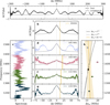 |
Fig. A.1. Scintillation analysis of FRB 20201020A. Panel (a) shows the ACF of the full spectrum of the FRB in black, with a grey solid line showing the fit of the central peak to a Lorentzian function. Panel (b) shows a zoomed-in version of the central 75 MHz of the ACF, with a yellow dashed line with shaded regions indicating the HWHM of the fitted Lorentzian. Panel (c) shows the spectrum of the FRB, with four different colours indicating the four sub-bands it was divided into. Panels (d), (e), (f), and (g) show the ACF of each of the four subbands of the spectrum, with colours matching the division of the spectrum, and the grey lines showing the fit of the central peak to a Lorentzian. The yellow dashed line with shaded contours marks the position of the HWHM. Finally, panel (h) gives the HWHM of each sub-band as a function of frequency. The coloured markers match the colours of the subbands, and the black marker indicates the HWHM over the whole spectrum. The black dashed line indicates the expected evolution with frequency for a power-law index α = 4.4, as expected from scintillation in the ISM. The grey line marks the fit of the four sub-band HWHMs to a power-law function, and the yellow line marks its fit to a linear function. |
The evolution of HWHM is not monotonic; the values of the highest and lowest sub-bands are lower than the intermediate sub-bands. This is likely explained by the low number of scintles within each sub-band and by the low S/N of the scintles of the intermediate sub-bands.
We fitted the frequency evolution of the decorrelation bandwidth to two different functions. A power-law function with power-law index 4.4 is expected from scintillation in the ISM with a Kolmogorov spectrum (Cordes et al. 1985). By fitting to a power law, we obtain Δνfl ∝ ν3.0, which differs from the expected power-law index. Additionally, we fit the Δνfl to a linear function, and find Δνfl = −6.25 × 10⁻³ν + 20.79. This would indicate that the decorrelation bandwidth increases at lower frequencies. The evolution of the FRB intensity fluctuations with frequency appears to be at odds with what is expected from scintillation in the ISM. However, the low number of scintles within the observing bandwidth does not allow us to confirm whether the frequency structure is intrinsic to the source or is instead produced by the propagation of the radio waves through the interstellar and intergalactic medium.
Decorrelation bandwidth of FRB 20201020A in different frequency ranges.
Appendix B: 2D auto-correlation functions of FRB 20201020A, A17 and A53
In this section, we show the 2D auto-correlation functions (ACF)8 of FRB 20201020A, A17 and A53 (Figs. B.1−B.3). After computing the ACFs, they were fitted to 2D Gaussians with an inclination angle. This inclination angle gives us a robust drift-rate estimate of the burst subcomponents Hessels et al. (2019). We obtained the time and frequency ACFs by averaging in frequency and time, respectively.
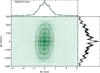 |
Fig. B.1. Two-dimensional ACFs of FRB 20201020A. The lower left panel shows the 2D ACF in green, and the 2D Gaussian fit as black elliptical contours. The top panel shows the frequency-averaged temporal ACF in black and the Gaussian fit in green. The left panels show the time-averaged ACF in frequency in black and the Gaussian fit in green. |
The HWHM of a Lorentzian fitted to the central peak of the frequency ACF gives the scintillation bandwidth of the FRB. In addition, any structure in the temporal ACF can provide us with information about any dominant timescales in the pulse structure.
Appendix C: Galaxies within the FRB error region
In this Appendix, Table C.1 shows the galaxies identified within the 99% confidence interval on the localisation of FRB 20201020A.
Galaxies within the error region of FRB 20201020A.
Appendix D: Rotation measure
In this section we show the results from the polarisation and Faraday rotation calibration, shown in Fig. D.1. Note that the best RM of 110 ± 69 pc cm−3 is close to the lower limit of what Apertif can measure given its central frequency and bandwidth.
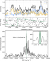 |
Fig. D.1. Measured polarisation properties of FRB 20201020A. The top panel shows the Stokes parameters I (black), Q (blue) and U (yellow) as a function of frequency, calibrated by assuming Stokes V to be zero. The second panel shows the measured phase between Q and U (black dots) and its fit in green. The bottom panel shows the RM-synthesis solution, with the polarised amplitude as a function of RM. The dashed green line marks the position of the maximum, at RM=+110 ± 69 pc cm−3. The inset shows the same, but zoomed in at the central peak of the polarised amplitude. |
Appendix E: Periodicity significances
Table E.1 gives the periodicity significance and percentiles of FRB 20201020A, the FRB 20180916Bbursts A17 and A53, and the CHIME FRBs 20210206A and 20210213A under different null hypotheses and simulated aperiodic subcomponent spacings, assuming different exclusion parameters η.
Statistical significance of burst periodicities in this study using different methods.
Appendix F: Maximal number of orbits in binary merger
To demonstrate that a binary merger cannot explain the morphology of FRB 20201020A, we computed the maximal number of orbits that a binary system could complete after reaching a frequency of 240 Hz. Following Cutler & Flanagan (1994, equation 16), we derived the analytical expression for the phase of the gravitational waveform as a function of time, ϕ(t), by solving the differential equation of  and integrating
  , where f(t) is the GW frequency. We computed the maximal number of orbits that could be completed between the time when the system reaches the FRB frequency and the time of the merger through the maximal phase difference Δϕmax, following the steps given below. We start with Eq. 16 from Cutler & Flanagan (1994):
 (F.1)
(F.1)
We define  , where ℳ ≡ μ3/5M2/5 is the chirp mass, M = M1 + M2 the total mass of the system and μ = M1M2/M the reduced mass. G is the gravitational constant and c the speed of light in the vacuum (we note that we do not make the replacement G = c = 1). We solve the differential equation to find f(t):
 (F.2)
(F.2)
Here, f0 is the frequency at t = 0. To get the orbital phase, we solve the differential equation  and we get:
 (F.3)
(F.3)
The value of 𝒞 is given by the initial conditions; ϕ(0) = 0 so we get  . In the simplest scenario where we assume the objects in the binary system to be point-like sources, the merger will happen when
  , from which we define the maximal orbital phase Δϕmax = 𝒞. Finally, we get the expression the maximal number of orbits between the FRB frequency and the time of the merger, assuming our initial frequency f0 to be the inverse of the FRB subcomponent separation fFRB:
 (F.4)
(F.4)
Here, ℳ ≡ μ3/5M2/5 is the chirp mass, with M = M1 + M2 the total mass of the system and μ = M1M2/M the reduced mass. G is the gravitational constant and c the speed of light in the vacuum. We computed Δϕmax for three values of M1 = 0.2, 1.4, 100 M⊙, and a range of M2 values between 0.2 M⊙ (close to the lowest mass WD; Kilic et al. 2007) and 100 M⊙. We tested both f0 = 2435 Hz and 4818 Hz as initial GW frequencies.
As shown in Fig. F.1, only a WD–WD system could complete four rotations (Δϕmax = 8π) after reaching fFRB = 4818 Hz. However, given the typical WD radius of 5000-10000 km, this is not a realistic scenario. Additionally, the expected separation between the two WD when reaching this frequency would be lower than their radius. As none of the systems with masses corresponding to a BNS or BHNS system could reach Δϕmax = 8π, we can discard the pre-merger scenario as an explanation for FRB 20201020A.
This FRB frequency could only be produced at the very last moments of the inspiral, right before the merger. At this stage, the frequency derivative would be very high, which translates to a perceptibly decreasing spacing between burst subcomponents.
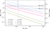 |
Fig. F.1. Maximal orbital phases a binary system can complete before a merger after reaching a GW frequency of 2435 Hz (solid lines) and 4818 Hz (dashed lines). The dashed and dotted black horizontal lines mark phases of 8π (four rotations) and 2π (one rotation), respectively, which are required to see five and three FRB subcomponents, respectively. The orbital phases were computed for binary systems with the mass of the first compact object being M1 = 0.2 M⊙ (blue), 1.4 M⊙ (pink) and 100 M⊙ (green), while the mass of the second object M2 ranges between 0.2 and 100 M⊙. The dot-dashed grey vertical line indicates M2 = 1.4 M⊙. |
All Tables
Statistical significance of burst periodicities in this study using different methods.
All Figures
|
Fig. 1. Dynamic spectrum of FRB 20201020A, de-dispersed to a DM of 398.59 pc cm−3. The top panel shows the average calibrated pulse profile of the burst, and the bottom panel the intensity of the burst in time versus frequency. The data have been downsampled in frequency by a factor 8. |
| In the text | |
|
Fig. 2. Localisation region of FRB 20201020A. The best position is indicated by a pink cross, and the 99% confidence interval contour is represented by the pink ellipse. Galaxies from the NED database within the error region are marked as blue crosses. The background is a composite colour image from SDSS (Blanton 2017). |
| In the text | |
|
Fig. 3. Timing analysis of FRB 20201020A (left column), A17 (central column), and A53 (right column). The top of panels (a), (e), and (i) shows the pulse profile of each burst (black) and the fitted multi-component Gaussians in green for FRB 20201020A and A53; for A17 the bright components are shown in blue and the dim components in yellow. The bottom of panels (a), (e), and (i) shows the residuals of the multi-component Gaussian fit of each pulse profile. Panels (b), (f), and (j) show the power spectra of each pulse profile in black. In (b), the vertical dashed line indicates the average separation of the FRB 20201020A components, while the blue line shows the Gaussian fit to the 2.4 kHz component. In (f), the blue and yellow lines show respectively the power spectra of the bright and dim components. Panels (c), (g), and (k) show the ToAs of all subcomponents as a function of component number. In most cases, the error on the ToAs is smaller than the marker size. The dashed green lines in (c), (g), and (k) are linear fits to the ToAs, and the lower panels show their residuals normalised by the mean subcomponent separation Psc. Panels (d), (h), and (l) show histograms of the simulated rχ2 statistic using a shifted Poissonian subcomponent spacing distribution with η = 0.2 to compute the significance of the periodicity. The vertical lines correspond to the rχ2 of the linear fit to the data. The significance is indicated as blue text. |
| In the text | |
|
Fig. 4. Subcomponent separation of FRB 20180916B multi-component bursts presented in Pastor-Marazuela et al. (2021). The top panel shows a histogram of the burst separation between discernible subcomponents in multi-component bursts. The mean A17 and A53 separations are shown as vertical dashed blue and yellow lines, respectively. The fit to a single lognormal and a double lognormal distribution are shown as solid and dotted black lines, respectively. The bottom panel shows the burst separations in each burst of the sample. |
| In the text | |
|
Fig. 5. Timing analysis of burst A53 from FRB 20180916B. Panel (a) shows the pulse profile of A53 as grey dots at 82 μs time resolution, and the smoothed profile as a black solid line. The yellow dots and solid line show the same for the off-burst signal. Panel (b) shows the residuals of the on- and off-burst signal as black and yellow lines, respectively. Green diamonds and dots show respectively the 5σ and 3σ outliers of the on-burst residuals. Panel (c) shows the distribution of the on-burst residuals in black and off-burst residuals in yellow. The yellow shaded regions, from dark to light, indicate the 1σ, 2σ, and 3σ contours of the off-pulse distribution fitted to a Gaussian. Panel (d) shows the power spectrum of A53 in black fitted to a power-law function shown in blue. The green dashed and yellow dotted lines mark the position of the mean component separation and the maximum of the residuals, respectively. Panel (e) shows the power spectrum residuals R(ν). Panel (f) presents the ACF of the light curve of A53 as a solid black line. The pink vertical lines indicate the separation between consecutive components, the green line the separation between the two brightest components, and the blue line the separation between the first and third brightest components. |
| In the text | |
|
Fig. 6. Neutron star mass–radius diagram. The solid lines represent the mass–radius relationship of typical EoSs. The grey shaded regions are forbidden by general relativity, finite pressure (P < inf), and causality. The yellow shaded region is forbidden by the rotation of the fastest spinning pulsar J1748−2446ad (Hessels et al. 2006). The red shaded region shows the mass of J0740+6620 (Cromartie et al. 2020; Fonseca et al. 2021) and the orange region the mass of J1614-2230 (Demorest et al. 2010), the two heaviest known NSs. Valid EoSs need to cross those regions. The green line and green shaded region would be forbidden if the quasi-period of FRB 20201020A were produced by the rotation of a NS at 2435 Hz, and the region to the right of the dashed green line would be forbidden if the rotation was at 1205 Hz. |
| In the text | |
|
Fig. A.1. Scintillation analysis of FRB 20201020A. Panel (a) shows the ACF of the full spectrum of the FRB in black, with a grey solid line showing the fit of the central peak to a Lorentzian function. Panel (b) shows a zoomed-in version of the central 75 MHz of the ACF, with a yellow dashed line with shaded regions indicating the HWHM of the fitted Lorentzian. Panel (c) shows the spectrum of the FRB, with four different colours indicating the four sub-bands it was divided into. Panels (d), (e), (f), and (g) show the ACF of each of the four subbands of the spectrum, with colours matching the division of the spectrum, and the grey lines showing the fit of the central peak to a Lorentzian. The yellow dashed line with shaded contours marks the position of the HWHM. Finally, panel (h) gives the HWHM of each sub-band as a function of frequency. The coloured markers match the colours of the subbands, and the black marker indicates the HWHM over the whole spectrum. The black dashed line indicates the expected evolution with frequency for a power-law index α = 4.4, as expected from scintillation in the ISM. The grey line marks the fit of the four sub-band HWHMs to a power-law function, and the yellow line marks its fit to a linear function. |
| In the text | |
|
Fig. B.1. Two-dimensional ACFs of FRB 20201020A. The lower left panel shows the 2D ACF in green, and the 2D Gaussian fit as black elliptical contours. The top panel shows the frequency-averaged temporal ACF in black and the Gaussian fit in green. The left panels show the time-averaged ACF in frequency in black and the Gaussian fit in green. |
| In the text | |
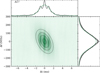 |
Fig. B.2. Same as B.1 but for A17. |
| In the text | |
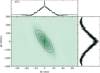 |
Fig. B.3. Same as B.1 but for A53. |
| In the text | |
|
Fig. D.1. Measured polarisation properties of FRB 20201020A. The top panel shows the Stokes parameters I (black), Q (blue) and U (yellow) as a function of frequency, calibrated by assuming Stokes V to be zero. The second panel shows the measured phase between Q and U (black dots) and its fit in green. The bottom panel shows the RM-synthesis solution, with the polarised amplitude as a function of RM. The dashed green line marks the position of the maximum, at RM=+110 ± 69 pc cm−3. The inset shows the same, but zoomed in at the central peak of the polarised amplitude. |
| In the text | |
|
Fig. F.1. Maximal orbital phases a binary system can complete before a merger after reaching a GW frequency of 2435 Hz (solid lines) and 4818 Hz (dashed lines). The dashed and dotted black horizontal lines mark phases of 8π (four rotations) and 2π (one rotation), respectively, which are required to see five and three FRB subcomponents, respectively. The orbital phases were computed for binary systems with the mass of the first compact object being M1 = 0.2 M⊙ (blue), 1.4 M⊙ (pink) and 100 M⊙ (green), while the mass of the second object M2 ranges between 0.2 and 100 M⊙. The dot-dashed grey vertical line indicates M2 = 1.4 M⊙. |
| In the text | |
Current usage metrics show cumulative count of Article Views (full-text article views including HTML views, PDF and ePub downloads, according to the available data) and Abstracts Views on Vision4Press platform.
Data correspond to usage on the plateform after 2015. The current usage metrics is available 48-96 hours after online publication and is updated daily on week days.
Initial download of the metrics may take a while.