| Issue |
A&A
Volume 677, September 2023
|
|
|---|---|---|
| Article Number | A66 | |
| Number of page(s) | 21 | |
| Section | Catalogs and data | |
| DOI | https://doi.org/10.1051/0004-6361/202346579 | |
| Published online | 05 September 2023 | |
NIKA2 Cosmological Legacy Survey
Survey description and galaxy number counts
1
Aix-Marseille Univ., CNRS, CNES, LAM (Laboratoire d’Astrophysique de Marseille),
Marseille, France
e-mail: This email address is being protected from spambots. You need JavaScript enabled to view it.
2
Université de Strasbourg, CNRS, Observatoire astronomique de Strasbourg, UMR 7550,
67000
Strasbourg, France
3
Université Côte d’Azur, Observatoire de la Côte d’Azur, CNRS, Laboratoire Lagrange,
Nice, France
4
School of Physics and Astronomy, Cardiff University, Queen’s Buildings, The Parade,
Cardiff,
CF24 3AA, UK
5
AIM, CEA, CNRS, Université Paris-Saclay, Université Paris-Diderot,
Sorbonne Paris-Cité,
91191
Gif-sur-Yvette, France
6
Univ. Grenoble Alpes, CNRS, Grenoble INP, LPSC-IN2P3,
53, avenue des Martyrs,
38000
Grenoble, France
7
Max-Planck-Institut fur Extraterrestrische Physik (MPE),
Giessenbachstr. 1,
85748
Garching, Germany
8
Institut Néel, CNRS, Université Grenoble Alpes,
France
9
Institut de RadioAstronomie Millimétrique (IRAM),
Grenoble, France
10
Observatoire Astronomique de l’Université de Genève,
Chemin Pegasi 51,
Versoix, Switzerland
11
Dipartimento di Fisica, Sapienza Università di Roma,
Piazzale Aldo Moro 5,
00185
Roma, Italy
12
Univ. Grenoble Alpes, CNRS, IPAG,
38000
Grenoble, France
13
Centro de Astrobiología (CSIC-INTA), Torrejón de Ardoz,
28850
Madrid, Spain
14
High Energy Physics Division, Argonne National Laboratory,
9700 South Cass Avenue,
Lemont, IL
60439, USA
15
Instituto de Radioastronomía Milimétrica (IRAM),
Granada, Spain
16
LERMA, Observatoire de Paris, PSL Research University, CNRS, Sorbonne Université, UPMC,
75014
Paris, France
17
IFPU-Institute for Fundamental Physics of the Universe,
Via Beirut 2,
34151
Trieste, Italy
18
INAF-Osservatorio Astronomico di Trieste,
Via Tiepolo 11,
34131
Trieste, Italy
19
School of Earth and Space Exploration and Department of Physics, Arizona State University,
Tempe, AZ
85287, USA
20
Laboratoire de Physique de l’École Normale Supérieure, ENS, PSL Research University, CNRS, Sorbonne Université, Université de Paris,
75005
Paris, France
21
INAF-Osservatorio Astronomico di Cagliari,
Via della Scienza 5,
09047
Selargius, Italy
22
Department of Physics and Astronomy, University of Pennsylvania,
209 South 33rd Street,
Philadelphia, PA
19104, USA
23
Institut d’Astrophysique de Paris, Sorbonne Université, CNRS (UMR7095),
Paris, France
24
University of Lyon,
UCB Lyon 1, CNRS/IN2P3, IP2I,
69622
Villeurbanne, France
Received:
3
April
2023
Accepted:
11
May
2023
Abstract
Context. Finding and characterizing the heavily obscured galaxies with extreme star formation up to very high redshift is key for constraining the formation of the most massive galaxies in the early Universe. It has been shown that these obscured galaxies are major contributors to the accumulation of stellar mass to z ~ 4. At higher redshift, and despite recent progress, the contribution of dust-obscured galaxies remains poorly known.
Aims. Deep surveys in the millimeter domain are necessary in order to probe the dust-obscured galaxies at high redshift. We conducted a large observing program at 1.2 and 2 mm with the NIKA2 camera installed on the IRAM 30m telescope. This NIKA2 Cosmological Legacy Survey (N2CLS) covers two emblematic fields: GOODS-N and COSMOS. We introduce the N2CLS survey and present new 1.2 and 2 mm number counts measurements based on the tiered N2CLS observations (from October 2017 to May 2021) covering 1169 arcmin2.
Methods. After a careful data reduction and source extraction, we develop an end-to-end simulation that combines an input sky model with the instrument noise and data reduction pipeline artifacts. This simulation is used to compute the sample purity, flux boosting, pipeline transfer function, completeness, and effective area of the survey (taking into account the non-homogeneous sky coverage). For the input sky model, we used the 117 square degree SIDES simulations, which include galaxy clustering. Our formalism allows us to correct the source number counts to obtain galaxy number counts, the difference between the two being due to resolution effects caused by the blending of several galaxies inside the large beam of single-dish instruments.
Results. The N2CLS-May2021 survey is already the deepest and largest ever made at 1.2 and 2 mm. It reaches an average 1σ- noise level of 0.17 and 0.048 mJy on GOODS-N over 159 arcmin2, and 0.46 and 0.14 mJy on COSMOS over 1010 arcmin2, at 1.2 and 2 mm, respectively. For a purity threshold of 80%, we detect 120 and 67 sources in GOODS-N and 195 and 76 sources in COSMOS at 1.2 and 2 mm, respectively. At 1.2 mm, the number counts measurement probes consistently 1.5 orders of magnitude in flux density, covering the full flux density range from previous single-dish surveys and going a factor of 2 deeper into the sub-mJy regime. Our measurement connects the bright single-dish to the deep interferometric number counts. At 2 mm, our measurement matches the depth of the deepest interferometric number counts and extends a factor of 2 above the brightest constraints. After correcting for resolution effects, our results reconcile the single-dish and interferometric number counts, which can be further accurately compared with model predictions.
Conclusions. While the observation in GOODS-N have already reached the target depth, we expect the final N2CLS survey to be 1.5 times deeper for COSMOS. Thanks to its volume-complete flux selection, the final N2CLS sample will be an ideal reference for conducting a full characterization of dust-obscured galaxies at high redshift.
Key words: galaxies: evolution / methods: data analysis / radio continuum: galaxies / submillimeter: galaxies
© The Authors 2023
 Open Access article, published by EDP Sciences, under the terms of the Creative Commons Attribution License (https://creativecommons.org/licenses/by/4.0), which permits unrestricted use, distribution, and reproduction in any medium, provided the original work is properly cited.
This article is published in open access under the Subscribe to Open model. This email address is being protected from spambots. You need JavaScript enabled to view it. to support open access publication.
1 Introduction
Blind far-infrared (far-IR) to millimeter (mm) observations have dramatically improved our understanding of the massive dusty galaxies in the early Universe (e.g., Blain et al. 2002; Lagache et al. 2005; Casey et al. 2014; Madau & Dickinson 2014; Hodge & da Cunha 2020). These sources are believed to be the progenitors of massive quiescent galaxies in dense environments that later emerged at lower redshift (Toft et al. 2014; Spilker et al. 2019; Valentino et al. 2020; Gómez-Guijarro et al. 2022b), and the study of the early phase of their formation and evolution provides a means to test theories of galaxy and structure formation and evolution (Liang et al. 2018; Lovell et al. 2021; Hayward et al. 2021). Following the commissioning of ground-based (sub)mm observations, they rapidly became one of the best ways to find the dusty galaxies at the highest redshift (e.g., Barger et al. 1998; Chapman et al. 2005; Ivison et al. 2007; Hodge et al. 2013; Strandet et al. 2017; Simpson et al. 2020; Dudzevičiūtė et al. 2020). Contrary to targeted follow-up observations of samples selected at shorter wavelengths (e.g., Capak et al. 2015; Béthermin et al. 2020; Bouwens et al. 2022), the dusty galaxy samples from blind far-infrared (far-IR) to (sub)mm surveys of continuous sky areas are much less affected by complex selection functions, and are therefore easier to interpret. There are also statistical studies on dusty star forming galaxies (DSFGs) using the serendipitously detected samples in targeted ALMA observations (Béthermin et al. 2020; Gruppioni et al. 2020; Venemans et al. 2020; Fudamoto et al. 2021). However, these studies are also subject to complex corrections due to clustering and are still limited by the area that can be covered by interferometric observations.
Deep and blind surveys are, in particular, ideal for measuring the source number counts, which describe the variation of the number density of sources as a function of their flux at given wavelengths. With limited information on individual sources, the number counts still provide constraints on the integrated number density of sources of different flux across cosmic time and accounting for the selection function is relatively straightforward in the analysis. Although semi-analytic models with simplified assumptions can make successful predictions as to the source number counts, hydrodynamical simulations have been struggling to reproduce this simple observable (Hayward et al. 2013; McAlpine et al. 2019) and are still in tension with observations within certain flux ranges (Lovell et al. 2021; Hayward et al. 2021). This indicates that detailed studies on smaller-scale physics, including the spatial distribution of dust and stars, the “burstiness” of star formation, as well as the initial mass function in (sub)mm bright dusty galaxies, are still essential to our understanding of the formation and evolution of high-z dusty galaxies (Hodge & da Cunha 2020; Popping et al. 2020).
Due to limitations on sensitivity or field of view, it is difficult for one blind survey alone to detect a statistically large sample of mm sources over a wide range of fluxes and make a complete measurement of the number counts. In practice, the measurements of the number counts of bright mm sources, that is, above a few mJy at 1.2 mm, are predominantly obtained using single-dish observations (e.g., Lindner et al. 2011; Scott et al. 2012). On the contrary, the Atacama Large Millimeter/submillimeter Array (ALMA) brings most of the constraints on the faint-end number counts at the sub-mJy regime, where single-dish surveys start to be limited by their sensitivity and source confusion (e.g., Fujimoto et al. 2016; González-López et al. 2020; Gómez-Guijarro et al. 2022a). Most previous studies directly combined the two different types of observations, interpreting them as an ensemble and using them in conjunction during model comparisons. However, it has also been shown that single-dish and interferometer surveys do not provide completely equivalent flux measurements (Hayward et al. 2013; Cowley et al. 2015; Scudder et al. 2016; Béthermin et al. 2017). The higher resolution of interferometers gives a flux estimate for individual galaxies, while the relatively large beam of single-dish observations leaves the possibility for contamination of the measured fluxes of the brightest “isolated” galaxy in the beam from close-by faint galaxies (Béthermin et al. 2017). Previous studies lack realistic estimations of the magnitude of this contamination based on real data from blind surveys. Its impact on the joint analysis of raw single-dish and interferometer number counts is seldom considered.
The New IRAM KIDs Array, NIKA2 (Monfardini et al. 2014; Calvo et al. 2016; Bourrion et al. 2016), offers a new promising path for statistical studies of the early stage of galaxy evolution obscured by dust. NIKA2 is a continuum instrument installed on the IRAM 30m telescope in October 2015 (Adam et al. 2018; Perotto et al. 2020). It allows observations within a 6.5′ diameter instantaneous field of view using three detector arrays in two bands simultaneously. These include two arrays with 1140 detectors at 1.2 mm (255 GHz), as well as another array with 616 detectors operating at 2 mm (150GHz). Thanks to the large collecting area and the large number of detectors filling a large instantaneous field of view, the combination of the 30m telescope and NIKA2 permits sensitive and efficient blind surveys of high-z DSFGs with an angular resolution of 11.1″ and 17.6″ at 1.2 and 2 mm, respectively (Perotto et al. 2020). This is the purpose of the NIKA2 Cosmological Survey (N2CLS). With 300h of guaranteed-time observations, N2CLS performs deep blind mappings in the GOODS-N and COSMOS field to make a systematical census of DSFGs from cosmic noon up to the first billion years of the Universe with both large area coverage and unprecedented depth among single-dish mm observations. The observations at these relatively long wavelengths are also expected to favor the selection of DSFGs at higher red-shift (Blain et al. 2002; Lagache et al. 2004; Casey et al. 2014; Zavala et al. 2014; Béthermin et al. 2015b).
In this paper, we introduce the N2CLS survey and present new 1.2 and 2 mm number counts measurements based on the tiered N2CLS observations over 1169 arcmin2 in GOODS-N and COSMOS. Here, we use data obtained until May 2021. At this date, the collection of GOODS-N data was complete, while COSMOS was still being acquired. Our measurements already cover an unprecedentedly wide range of source fluxes from one single-dish instrument and consider the impact of the beam in number counts measurements for the first time. This is achieved using a dedicated end-to-end simulation based on the SIDES-UCHUU model (Gkogkou et al. 2023). The paper is organized as follows. In Sect. 2 we introduce the survey strategy, present the N2CLS maps, and describe the method of source extraction and photometry. In Sect. 3 we describe the framework for the correction of the bias in source detection and flux measurement due to instrument noise, the pipeline transfer function, and the large beam. Section 4 presents the 1.2 and 2 mm source number counts measurements and their comparison with previous observations. We also determine the galaxy number counts, which are derived from the source number counts and our end-to-end simulation based on realistic sky simulations, including the clustering. These galaxy counts are finally compared with model expectations. In Sect. 5, we discuss the modeling of the mm number counts and the impact of spatial resolution on flux measurements in single-dish observations. We finally conclude in Sect. 6.
2 Survey description, data reduction, and source extraction
2.1 Survey design and observation
The N2CLS was designed to have good statistics on both faint and bright sources through a narrow and deep observation in the GOODS-N field and a wider and shallower observation in the COSMOS field. In GOODS-N, the survey time was chosen to approach the source confusion limit of the IRAM 30m telescope at 1.2 mm on an area of ~160 arcmin2. Source confusion is the contribution to noise in an image due to the superimposed signals from faint unresolved sources at the scale of the observing beam, and was estimated using the model from Béthermin et al. (2012) and considering a source density of 1/20Ω. Values (5σconf) are about 0.68 mJy and 0.23 mJy at 1.2 and 2 mm, respectively, for FHWM of 12 and 18″. In COSMOS, N2CLS covers a much larger area of ~1000 arcmin2 with a shallower depth, and is designed to cover a larger sample of brighter sources, biased towards higher redshifts (which is counterintuitive; see Béthermin et al. 2015b). Thanks to the dual-band coverage of NIKA2, we simultaneously obtain 1.2 and 2 mm data from the N2CLS observations.
N2CLS observations started in October 2017 and finished in January 2023, under project ID 192-16. For the work presented here, we use 170.85 h on-field observations in total, which were conducted from October 2017 to March 2021. These represent 86.15 h on GOODS-N and 84.7 h on COSMOS. For the GOODS-N observations, we executed two groups of 12.0′×6.3′ and 6.5′×12.3′ scans in orthogonal directions centered on RA=12:36:55.03 and Dec=62:14:37.59. For the COSMOS field, we carried out two groups of 27.0′×34.7′ and 35.0′×28.0′ orthogonal on-the-fly scans centered on RA=10:00:28.81 Dec=02:17:30.44. The two groups of orthogonal scans in both fields were taken at equal times. In GOODS-N, we made the two groups of scans with a speed of 40 and 35 arcsec s−1, and position angles of −40° and −130° in the RA-DEC coordinate system of the telescope. For COSMOS, the two groups of scans were observed with a speed of 60 arcsec s−1 at position angles of 0° and +90° in the RA–Dec coordinate system of the telescope.
Observations were conducted with a mean line-of-sight opacity  of 0.27 and 0.25 for GOODS-N and COSMOS, respectively, where τ225 GHz is the zenith opacity deduced from the Pico Veleta tau-meter measurement at 225 GHz.
2.2 Data reduction
The N2CLS data are reduced using the “may21a”1 version of the PIIC data reduction pipeline developed and supported by IRAM (Zylka 2013). Our data reduction script is adapted from the default template provided with the PIIC software. We use the options “deepfield” and “weakSou”, which are designed to recover faint sources from the NIKA2 timeline data without prior information on source positions. We used the PIIC iterative procedure with five iterations to recover the bright source fluxes by subtracting an estimate of the sky (so-called “source map”) constructed by thresholding the previous iteration map at 4σ. The procedure converges rapidly and five iterations are sufficient. At each iteration, following the default PIIC parameters, the emission of the sky is subtracted from the timeline using the 16 best-correlated KIDs. The signal is also corrected for sky opacity using the IRAM Pico Veleta tau-meter measurements extrapolated to the NIKA2 bands. Additionally, for GOODS-N and COSMOS, we set the order of polynomial function used for baseline correction (parameter “blOrderOrig” in PIIC) to 10 and 17, respectively, which removes residual fluctuations in the signal map (such as atmospheric and electronic residual fluctuations). All of the data from array 1 and array 3 are reduced together to produce a single 1.2 mm map, while the data from array 2 are used to produce the 2 mm map. With its optimized re-gridding strategy applied to redistribute the KIDs signal, PIIC properly samples the Gaussian response of point-like sources with 3″ and 4″ sized pixels at 1.2 and 2 mm. The resulting FWHM of the point sources in the final 1.2 and 2 mm maps are 11.6″ and 18.0″, respectively.
A scan selection is performed by PIIC before the data reduction, which automatically discards the bad scans based on their noise properties (e.g., higher noise linked to weather instabilities). We have 762 and 394 scans in total for GOODS-N and COSMOS, respectively. Each scan generates three data files with one for each array. At 1.2 mm (2 arrays), among the 1524 and 788 data files on GOODS-N and COSMOS, PIIC finally keeps 1281 and 700 files for map making. This represents a total on-source time of 78.0 h and 78.7 h in GOODS-N and COSMOS, respectively. At 2.0 mm, 599 and 351 data files from GOODS-N and COSMOS observations are used to produce the maps, respectively. This corresponds to 72.8 h and 79.0 h on-source time in the two fields. The 225 GHz zenith opacities are ranging from 0.06 to 0.91 and elevations from 20° to 73°. Median opacities are equal to 0.2 for both fields.
In Figs. 1 and 2, we show the 1.2 and 2 mm signal-to-noise ratio (S/N) maps of the N2CLS survey in GOODS-N and COSMOS, which have been match-filtered by the beam in the corresponding band. The instrument noise maps are also generated from the weight maps produced along with the signal maps, and are also presented in Figs. 1 and 2 for 1.2 and 2 mm observations, respectively. Considering the high noise level on the edges, our study is restricted to the high-S/N regions delimited by the red lines. These regions are defined as having an instrument noise (σinst) smaller than 3 and 1.6 times the minimum value at the center of the GOODS-N and COSMOS field, respectively. This choice was made in order to achieve a compromise between homogeneity and maximization of the survey area. The high-quality regions used in our analysis cover 159 arcmin2 and 1010 arcmin2 in GOODS-N and COSMOS, respectively.
In Fig. 3, we present the distribution of the pixel values of the S/N map within the high-quality region of each field and each band. The S/N histograms reveal positive tails of high-S/N pixels, which indicates that sources are detected by the N2CLS survey. In Table 1, we provide the central instrument noise level of maps for each field and band. As the noise in the map is not uniform (especially for GOODS-N), we also provide the average instrument noise level in Table 1. In the high-quality regions of GOODS-N, the 1.2 and 2 mm maps have average noise levels of 0.17 mJy, and 0.048 mJy, respectively. For the COSMOS field, we have average noise levels of 0.46 mJy and 0.14 mJy within the high-quality regions at 1.2 and 2 mm, respectively.
In Table 1, we also compare the noise levels of N2CLS with those of previous surveys. To compare the noise level (in root mean square, or RMS) with surveys at different wavelengths from N2CLS, we rescaled it assuming a far-IR spectral energy distribution (SED) template of a typical star-forming galaxy at z = 2 from Béthermin et al. (2015a). In GOODS-N, N2CLS is surpassing the depth of any other single-dish mm survey with a similar size for wavelengths longer than 1 mm (Perera et al. 2008; Lindner et al. 2011; Staguhn et al. 2014); it currently matches the deepest SCUBA2 850 µm survey (Cowie et al. 2017) after taking into account the SED correction. As for COSMOS, N2CLS is 2.7 and 2.2 times deeper than AzTEC (Aretxaga et al. 2011) and MAMBO (Bertoldi et al. 2007) at 1.1/1.2 mm, respectively, and 1.6 times deeper than GISMO at 2 mm on a four times larger area (Magnelli et al. 2019). Similarly, in COSMOS field, N2CLS also reaches a depth comparable to the deepest SCUBA2 observation at 850 µm (S2COSMOS, see Simpson et al. 2019).
To obtain realizations of the instrument noise as closely as possible to the noise in real observations, we generate half-difference maps from the original scans. The half-difference maps, or null maps, are built by opposing half of the single-scan maps, that is, multiplying them by −1, and co-adding all of them. The opposed single-scan maps are selected randomly from the full list. The random selection and coadding operations are carried out by the HalfDifference module in nikamap (Beelen 2023)2. This process removes the astrophysical signal and preserves the instrument noise properties if the noise has symmetric properties. At first order, this hypothesis is valid with respect to atmospheric fluctuations, tuning variations, and electronic noise or even magnetic fields induced by the telescope, but could be challenged by beam distortions from telescope geometry or differential acceleration during the scans. We neglect the latter as we are not able to characterize their potential effects on the half-difference maps. We note that there is also a small potential bias due to the weight of each individual map, which could slightly favor positive or negative signals. Nevertheless, given the large number of individual scans and the generation of several realizations, this weight imbalance is minimized. The distribution of S/N in half-difference maps is shown in Fig. 3 along with its best fit by a normal distribution.
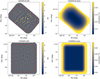 |
Fig. 1 Maps of signal-to-noise ratio (left panels) and noise (σinst in mJy/beam, right panels) of the 1.2 mm N2CLS maps of the GOODS-N (upper panels) and COSMOS (lower panels) fields. The S/N maps and noise maps are matched filtered (see Sect. 2.3). The regions enclosed in the red contours (159 arcmin2 for GOODS-N and 1010 arcmin2 for COSMOS) have sufficiently low noise to be analyzed by our source-detection algorithm, and our catalogs and number counts are derived only in these areas (see Sects. 2.3 and 4). |
2.3 Source extraction
The source detection of the N2CLS survey is made on the matched-filter PIIC maps produced by the dedicated Python package nikamap. For the matched filter, the kernels are fixed to circular 2D Gaussian with an FWHM equal to the corresponding beam sizes. The absolute level of the matched-filter maps is undefined, and any baseline residual in the PIIC maps could introduce a shift in the matched-filter signal map. Moreover, the PIIC re-gridding introduces a correlation in the weight maps, which needs to be taken into account. In order to retrieve a signal-to-noise ratio standard deviation of unity, and a null mean, assuming a Gaussian noise distribution, we perform a Gaussian fitting on the S/N pixel histogram values between −3 and 1.5 in order to avoid contamination by the sources. The best-fit parameters provide the global offset of the background and scale of the matched filter S/N pixel values, which are measured by the center (μS /N) and the width (σS /N) of the best-fit Gaussian function. Slight variations from unity are expected in the case of residual correlated noise in the maps or small bias in the absolute background value. We therefore normalize the noise maps by σS /N to have a unity standard deviation in the S/N map:
 (1)
(1)
where Ncorr is the noise map after this correction and Nori is the original noise map. Similarly, we correct the S/N maps using
 (2)
(2)
where S/Ncorr is the corrected S/N map and S/Nori is the original S/N map.
In the absence of noise, a matched-filter S/N map of an isolated point source is maximal at the position of the source. The nikamap package incorporates the find_peak algorithm from the photutils package (Bradley et al. 2022) to identify peaks above a certain threshold in the matched-filter S/N maps. We set an extraction box size to 5 pixels, allowing only the brightest source in a 2.5-pixel distance on both axes to be extracted. The box size is chosen to be matched with the FWHM of the PSF. The values at the position of detection in the beam matched-filter S/N maps provide the S/N of the point sources. We finally perform PSF-fitting photometry on the original PIIC signal maps (which are shown in Appendix A) with the nikamap package based on the BasicPSFPhotometry module in photutils. The position of the sources is fixed and corresponds to the results of find_peak. The PSFs used in this process are two-dimensional circular Gaus-sians that have their FWHMs defined by the beam described in the PIIC data products. The backgrounds of the maps are estimated by the MedianBackground module in photutils and are removed during the analysis.
For the source detection in the N2CLS observations, we further refine the choice of detection threshold in both fields and bands according to the purity analysis presented in Sect. 3.2. We use the source fluxes from the PSF fitting in the following analysis, which provide more robust flux measurements on slightly blended sources than the peak flux. As for the flux uncertainties, we provide the pixel value of the noise map after corrections (Eq. (1)), which accounts for the noise correlations between nearby pixels. However, we note that this does not take into account the additional uncertainties caused by degeneracies between the individual fluxes of heavily blended galaxies, but this is not a problem because we do not deblend sources closer than 2.5 pixels.
3 Characterization of the source-extraction performances
3.1 The simulation framework
In far-IR and mm blind surveys, flux measurements on individual sources and source number counts estimates are affected by systematic effects from data reduction, source detection, and flux measurement. Various methods were developed in previous studies to estimate and correct these effects. These include Bayesian techniques measuring the posterior distribution of source fluxes detected above a certain S/N and under a given source number count, which was applied in early single-dish surveys (Coppin et al. 2005). Some more recent studies turn to more empirical methods. They generate a series of pure-noise half-difference maps produced by randomly inverting the signal in half of the data or subscans and injecting sources into them following a given galaxy number count. The source detection and flux measurement procedure are then repeated, the deviation of the output flux from the input flux is estimated and compared to other properties, and the correction is applied to the real source catalog (e.g., Geach et al. 2017; Liu et al. 2018; Zavala et al. 2021). Empirical methods are also applied to estimate the false detection rate and the completeness at a given flux or S/N, which are then applied to the estimate of source number counts.
The Bayesian technique and empirical methods in previous studies mainly accounted for the impact of instrument noise on source detection and flux measurement. In addition to the instrument noise, previous studies also pointed out that astro-physical clustering and random alignments of sources inside the beam could also have a non-negligible impact on detected source fluxes in the ~3 m (far-IR), ~ 15 m (sub-mm), and ~30 m (mm) single-dish observations (Béthermin et al. 2017).
In addition, we also need to quantify the impact of the filtering resulting from the data reduction pipeline on the source fluxes, that is, the transfer functions. These transfer functions were first measured for NIKA by Adam et al. (2015) and further explored for the reduction of NIKA2 observations of the Sunyaev-Zeldovich effect in galaxy clusters (e.g., Muñoz-Echeverría et al. 2023). Our N2CLS observations, which are designed to detect faint point sources in deep fields, use different data reduction methods and we therefore need to measure our own transfer function.
PIIC offers the possibility to inject artificial sources – or an artificial sky map – into the timelines (since its “May21” version), allowing us to take into account the impact of both instrument noise and pipeline artifacts. A beam-convolved, noiseless sky model in the corresponding band is used as an input. The sky model is then translated into timelines of individual NIKA2 KIDs. The noiseless timeline from each KID are then combined with data from real calibrated observations with signs flipped on every other map. This process generates timeline data that resemble NIKA2 observations of the modeled sky region with the same depth as real observations but free from real astrophysical signals. These data are then reduced using the normal PIIC data reduction pipeline to produce simulated N2CLS-like maps. In the PIIC reduction and map construction with simulated timelines, we use the same parameters as for the reduction of N2CLS observations (see Sect. 2.2).
The input sky model is provided by the simulated infrared dusty extragalactic sky (SIDES; Béthermin et al. 2017, 2022) simulation. We use the SIDES light cone based on the Uchuu dark-matter simulation (Ishiyama et al. 2021) presented in Gkogkou et al. (2023). For each dark-matter halo, galaxy properties are generated following empirically measured scaling relations. The 1.2 and 2 mm fluxes are then derived using the NIKA2 bandpass, and maps are produced based on the fluxes and positions of all galaxies. The maps are then smoothed to the resolution of NIKA2 at the corresponding wavelength, as required by the PIIC simulation. Using a dark matter simulation, we obtain simulated sky maps with realistic galaxy clustering between sources, which is not accounted for in the techniques used in most of the previous studies. From the 117 deg2 simulation, a total of 117 independent tiles of 1 deg2 are used to produce the input sky model at 1.2 and 2 mm – simulating the GOODS-N and COSMOS fields –, which later produce 117 independent simulated N2CLS observations at the two wavelengths on the two fields. For each simulation, the scans list is shuffled before being read by PIIC. This ensures the noise realizations are independent in the 117 simulations of each field.
From the 117 input sky models for each field and band, we also obtain two sets of catalogs. The “galaxy catalogs” record the fluxes assigned to each simulated galaxy, blended or not with nearby galaxies in the NIKA2 beam. From the noiseless beam matched-filter model map, we also identify all peaks above a certain peak flux and record their position and peak fluxes in the “blob catalogs”. The peak flux thresholds are set to 0.15/0.05 mJy for GOODS-N and 0.45/0.15 mJy for COSMOS for input maps of simulation at 1.2/2 mm. These thresholds are comparable to the noise levels in the corresponding NIKA2 maps (see Table 1), and are below the detection limits in the noisy simulated maps.
In the analysis of completeness, purity, and flux correction, we use the input “blob catalog” as the reference, which is subject to the same source blending at the same NIKA2 angular resolution. The galaxy catalog is used to correct the impact of source blending on the number counts, as described in Sect. 4.3.
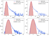 |
Fig. 3 Pixel S/N distribution within the high-quality regions of the 1.2 and 2 mm maps shown in Figs. 1 and 2, as well as the average distribution of pixel S/N in 100 randomly generated half-difference maps for each field and waveband (see Sect. 2.2). The red-shaded region illustrates the best-fit normal distribution on the average histograms of the half-difference maps. |
Comparison of N2CLS-May21 depth to other single-dish (sub)mm surveys in GOODS-N and COSMOS, which are all given as 1σ of the noise level.
3.2 Purity of detection
We first use the 117 simulated observations to determine the purity of the extracted source candidate sample. The purity is defined as the probability that a source extracted from the simulated output map is real. In practice, we consider that an extracted source is real if it can be matched with a source from the input blob catalog. The matching radius in position is 0.75 times the FWHM of the Gaussian beam of each NIKA2 band, which is consistent with the distance threshold used in previous studies (Geach et al. 2017). The same threshold of source cross-matching is used to estimate the source completeness (see Sect. 3.4), which ensures the two effects are consistently accounted for in the following estimate of source number counts. As described in Sect. 3.1, we limit the cross-matching to sources above a certain flux level in the input catalog. In cases where multiple catalog sources fall within the matching radius, we recognize the brightest source as the counterpart in the following analysis.
We present the purity as a function of S/N in Fig. 4. The results are fitted by a spline function. In COSMOS, the purity at 1.2 and 2 mm reaches 80% at S/Ncorr = 3.8, and is >95% at S/Ncorr > 4.6. In GOODS-N, the purity at 1.2 and 2 mm reaches 80% at S/Ncorr = 3.0 and S/Ncorr = 2.9, respectively, and reaches >95% at S/Ncorr > 4.2 and S/Ncorr > 4.1. The noise level is lower in GOODS-N than in COSMOS. The source density is therefore higher in GOODS-N at the fixed S/N threshold, while the number density of spurious sources is similar for the same S/N threshold. Therefore, any given purity is achieved with a lower S/N threshold in GOODS-N than in COSMOS. This analysis allows us to set the S/N detection threshold to reach a 80% purity in each field and wavelength. For the number counts (Sect. 4.1), the contamination by spurious sources can be corrected statistically and we therefore choose a purity of 80% so as to have corrections of 20% at most. In contrast, a >95% purity could be considered to select sources for follow-up observations.
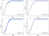 |
Fig. 4 Purity of detected sources at different S/N in the matched-filter map from the simulations at 1.2 and 2 mm in the GOODS-N (top panels) and COSMOS (lower panels) fields. |
3.3 Effective flux boosting
We also have to evaluate the impact of noise and data reduction (pipeline transfer function) on the measured source fluxes. We estimate these effects by comparing the recovered flux to the input flux for each blob of our simulation.
Like most blind single-dish deep-field surveys in the far-IR and mm, our blind detection algorithm uses only S/N as a threshold parameter. Considering the existence of noise in the real data, this method naturally biases detections toward sources that coincide with noise peaks. This boosts faint source fluxes above the threshold and leads to systematically overestimated fluxes for these objects. This effect is called “flux boosting”.
Apart from the flux-boosting effect, the PIIC pipeline could filter out a fraction of the source flux density. As explained in Sect. 2.2, PIIC is using the most correlated KIDS to estimate and remove sky noise per KID. An additional polynomial baseline is removed per subscan to correct for remaining instabilities. Due to the iterative mode of the data reduction (which is based on an S/N threshold to build a “source map”), sources at lower S/N are more affected by filtering effects than sources at higher S/N.
A proper correction of the combination of all the effects on source flux measurements is crucial in order to estimate source number counts. However, a detailed analysis of the contribution of each effect is beyond the scope of this work. In the present study, we directly measure the effective ratios between flux densities measured in the simulated maps and those in the input blob catalogs and study the variation of the ratios with S/Ncorr. Both the flux boosting and the pipeline filtering contribute to the deviation between input and output fluxes, and we refer to this output-to-input flux ratio as effective flux boosting in the following part of this paper. To estimate the effective flux boosting of source detection for each field and at each wavelength, we cross-match the input blob catalogs to the sources detected by our extraction algorithm in the output simulated maps. An input blob is considered to be recovered by our detection algorithm if any source above the S/N threshold (see Sect. 3.2) can be found within 0.75×FWHM of its position. If multiple input blobs correspond to the same detection, we use the closest one.
The distributions of the effective flux boosting are presented in Fig. 5. We note that the variation of median effective flux boosting between regions with different noise levels is small compared to the scatter. We therefore only focus on the variation of effective flux boosting as a function of S/Ncorr in the following analysis and discussion.
The mean effective flux boosting for both bands in the COSMOS field is mostly above one, suggesting that it is mainly dominated by flux boosting due to instrumental noise. The mean effective flux boosting curve also well matches the functional correction used by the S2CLS survey (Geach et al. 2017), which only accounts for the typical flux boosting in their simulation. Contrary to COSMOS, the mean effective flux boosting in the GOODS-N field drops below unity even at relatively high S/N and reaches ~0.8 at the S/N used as the detection limit in both bands. This suggests a much stronger filtering effect on source flux densities by the data reduction pipeline.
In Fig. 5, we also notice a significant scatter in the ratio between input and output fluxes, especially at low S/N. The interquartile range is as high as 40%–80% at the S/Ncorr ~ 4, and drops to ~10% or less at S /Ncorr > 20. Even if we know the average correction to apply as a function of S/Ncorr, there are large uncertainties on this correction at low S/Ncorr. In Sect. 4.1, we discuss how this is taken into account to derive the number counts.
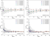 |
Fig. 5 Ratio between the source fluxes measured in the output simulated maps (fout) and the source fluxes from the input blob catalog (ftrue) as functions of S/N at 1.2 mm (left panels) and 2 mm (right panels) in GOODS-N (upper panels) and COSMOS (lower panels). This corresponds to the effective flux boosting described in Sect. 3.3. The boxes shown for each S/N bin represent ranges between 25% and 75% of the cumulative distribution and the upper and lower bounds of error bars present 5% to 95% of the cumulative distribution (within 1σ). The width of each box corresponds to the width of the corresponding S/Ncorr bin. The red dotted line shows the position of unity effective flux boosting as a reference for each plot. In addition, we use color-coded solid-filled circles to present the median flux boosting in regions with different noise levels. |
3.4 Completeness
Another important part of information to derive the number counts from our survey is the completeness of our catalogs. Completeness is defined as the probability of finding a source in the output catalog as a function of its input properties; for a heterogeneous survey, it can also vary depending on the position of the source. As our sources are unresolved, we consider only the input blob flux density (ftrue) as a relevant physical parameter. Concerning the variable linked to the survey, it is mainly driven by the instrument noise level at the source position (σinst).
In practice, completeness is evaluated as the fraction of input blobs at a given flux density (ftrue) that are recovered in the output catalog. The completeness curve varies significantly if we compute it in regions with different noise levels. However, by computing the completeness as a function of ftrue/σinst, that is, the input flux divided by the noise level at the source position, we find a similar completeness function in all regions, as shown in Fig. 6. This highlights that completeness is a function of two main parameters: ftrue and σinst. We fit our results using the following functional form:
 (3)
(3)
where C is the completeness, and x0 and y0 are free parameters. In our case, x is ftrue/σinst. These best fits are used below to derive the completeness of sources at given fluxes and compute their corresponding effective area of the survey (Sect. 3.5).
With the purity, effective flux boosting, and completeness correction functions set, here we summarize the properties of the N2CLS sample from blind detection for the following analysis in the paper. With the S/N thresholds of 80% purity set in Sect. 3.2, we detect 120 and 195 sources at 1.2 mm and 67 and 76 sources at 2 mm in GOODS-N and COSMOS, respectively. In the 1.2 mm maps of GOODS-N and COSMOS, we detect sources as faint as 0.4 mJy and 1.7 mJy in uncorrected PSF fluxes, respectively. At 2 mm, we reach limiting uncorrected PSF fluxes of 0.1 mJy and 0.5 mJy in GOODS-N and COSMOS, respectively.
The GOODS-N sample includes 44 sources with both 1.2 mm and 2.0 mm detections, 76 sources with only 1.2 mm detections, and 23 sources with only 2.0 mm detections. The COSMOS sample includes 49 sources with both 1.2 mm and 2.0 mm detections, 146 sources with only 1.2 mm detections, and 27 sources with only 2.0 mm detections. This large number of sources detected only at 2 mm may seem surprising considering the model forecasts, and is discussed in Sect. 5.3.
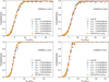 |
Fig. 6 Completeness of sources in N2CLS as a function of the ratio between source flux density and instrumental noise level (ftrue/σinst) at 1.2 mm (left panels) and 2 mm (right panels) in GOODS-N (upper panels) and COSMOS (lower panels). The completeness in various survey areas with different instrumental noise levels is presented as bluish color-coded dots, and the average completeness over the whole survey area is shown using oranges dots. The red line shows the best fit of the average completeness using the functional form of Eq. (3). |
3.5 Effective survey area
To derive the surface density of sources (also called number counts, see Sect. 4), we need to know the surface area of our survey. However, the survey has no clear border, because faint sources are unlikely to be detected in the noisy outskirts of the field. To take this into account, we use a similar method to that described by Béthermin et al. (2020). At a given source flux density, sources with their positions at different pixels in the map are expected to have different completeness of detection. The effective area is then the sum of the surface area of each pixel (Ωpix) multiplied by the completeness at the pixel position,
 (4)
(4)
where  is the completeness expected for a hypothetical source with a true flux density S. In practice, S is not known and we use the deboosted flux density as a proxy, which is the raw flux corrected by the expected effective flux boosting factor at the S/N of detection (see Sect. 3.3). The σi value is the instrument noise level in the ith pixel. This quantity varies with the source flux density, because fainter sources are less likely to be detected in the noisy edge of the map. Sources with lower flux densities will therefore have smaller effective areas.
This computation naturally accounts for the nonuniform depth within the N2CLS maps. It is especially crucial for our number counts analysis in the GOODS-N field, where we have a variation in survey depth of up to a factor of three across the region considered for number counts analysis.
4 Number counts
4.1 Derivation of the source number counts
The surface density of sources per observed flux density interval, or the differential source number count (dN/dS), is a simple measure of redshift-integrated source abundance, and has been used as a powerful tool to test and compare galaxy evolution models (e.g., McAlpine et al. 2019; Lagos et al. 2020; Lovell et al. 2021). We derive the differential source number counts at 1.2 and 2 mm in a given flux density bin using:
 (5)
(5)
where Ƥj and Ωeff,j are the purity and effective survey area of the j-th source of the extracted catalog with a flux density inside the bin (see Sects. 3.2 and 3.5, respectively), and ∆S is the width of the flux bin.
We also derive the corresponding cumulative source number counts (N(> S)). These are defined as the surface density of sources above a certain flux density higher than a given value, and are estimated using
 (6)
(6)
Contrary to the differential number counts, we sum all the sources with a flux density above a certain threshold instead of only those in the bin.
As discussed in Sect. 3.5, we use the deboosted flux density as a proxy for the true flux density in the computation of the effective survey area. To take into account the effect of the uncertainties on the deboosting factors, we perform 100 Monte Carlo realizations in which we draw a deboosting factor from the distribution and derive the deboosted flux density for each source, and finally compute the number counts accordingly. The median of the number counts realization is used to determine the central value and the 16th and 84th percentiles are used to compute the uncertainties. Finally, we combine these uncertainties quadratically from our Monte Carlo method with Poisson uncertainties.
To derive the differential number counts, we choose a common flux density binning for GOODS-N and COSMOS in order to facilitate the subsequent combination of the two measurements. The lower bound of the faintest bin is defined to have at least 50% completeness in the deepest field (GOODS-N). This corresponds to 0.60 and 0.20 mJy at 1.2 and 2 mm, respectively. The upper bound of the brightest bin is set to a slightly higher value than the brightest source of the survey. This corresponds to a flux density of 9.0 and 2.5 mJy at 1.2 and 2 mm, respectively. We use a uniform logarithmic sampling of this range. The number of bins is a compromise between a good sampling in flux density and a sufficient number of sources per bin to have reasonable uncertainties. We use 14 and 8 bins at 1.2 and 2 mm, respectively. In the faintest bins (5 bins at 1.2 mm and 3 bins at 2 mm), the completeness in the wider but shallower COSMOS field is well below 50%. Large and unreliable corrections are therefore necessary, and for this reason we do not compute the number counts in this regime for this field. In the brightest bins (5 bins at 1.2 mm and 3 bins at 2 mm), GOODS-N is too small to contain any source and number counts cannot be derived.
The cumulative number counts are derived using a similar method. The lower bounds of the differential number counts bins are used as flux density limits. Our results are summarized in Tables 2 and 3.
4.2 Validation of the number count reconstruction from simulations
Before comparing our number counts with previous observations, we perform an end-to-end simulation of the full analysis process to validate its accuracy. We therefore apply the same exact algorithm that we used to derive the number counts from our 117 simulated fields based on SIDES (see Sect. 3). These simulations therefore include all the possible instrumental effects, such as the transfer function of the map making or the source-extraction biases. We derive the source number counts by combining the 117 simulated fields to obtain output number counts with low uncertainties. We also derive the source counts from each individual simulated field to derive the field-to-field variance (also referred to as cosmic variance in the literature).
In Fig. 7, we compare these output number counts from our end-to-end simulation (blue squares) with the input source number counts derived from the blob catalog extracted from the noiseless SIDES maps (blue solid line, see Sect. 3.1 for the description of blob catalogs). The input and output results agree at 1 σ, except for the mild (<20%) disagreement in the faintest GOODS-N bin at 2 mm. This demonstrates the robustness of our method to derive source number counts.
We also compared the source number counts from our simulation and the N2CLS data (red diamonds). These always agree to within 2 σ and the majority of the data points are in the 1 σ range. The SIDES simulation is therefore very close to the real observations. This justifies a posteriori the choice of this simulation to characterize the map making and the source-extraction effects.
However, we can see that there is a small systematic offset between the simulation and the observations with GOODS-N being lower than SIDES and COSMOS being higher. This could be caused by the field-to-field variance, because flux bins are usually correlated (see e.g., Gkogkou et al. 2023 for the case of line-luminosity functions). We derived the 1 σ range of the number counts from the 117 SIDES realizations and found that the offset between N2CLS and the simulation is of the order of 1 σ of the field-to-field variance (the blue shaded region in Fig. 7). The field-to-field variance could therefore explain the small offset between the N2CLS counts in the two fields.
Differential and cumulative source number counts at 1.2 mm in GOODS-N and COSMOS.
4.3 From source to galaxy number counts
In Sect. 4.2, we show that we are able to measure the source counts reliably from the N2CLS data. However, as shown in Fig. 7, the galaxy number counts in the simulation (black dashed line) are lower than the source number counts (blue solid line). This difference is mainly due to the blending of several sources inside the ~ 10–30″ beam of single-dish instruments (Hayward et al. 2013; Cowley et al. 2015; Scudder et al. 2016). This effect has been extensively studied using the SIDES simulation in Béthermin et al. (2017).
We use the SIDES simulation to compute the conversion factor to apply to the source counts to derive the galaxy counts. This multiplicative correction factor is denoted Rdif for the differential number counts and Rcum for the cumulative number counts, and is estimated using the ratio between the SIDES intrinsic galaxy number counts and the SIDES source counts derived from the noiseless blob catalog. The values of these corrections are summarized in Tables 2 and 3.
Finally, we derive the mean of the galaxy number counts in the flux density range where data from the two fields overlap. We use an inverse-variance-weighted average of galaxy number counts in each field. For the bright and faint ends, we directly use the measurements in COSMOS and GOODS-N fields, respectively. The values and uncertainties of the combined 1.2 and 2 mm galaxy number counts are given in Table 4.
4.4 N2CLS number counts and comparison with previous observations
4.4.1 Internal consistency of N2CLS number counts
As demonstrated in the previous sections, we can reliably derive source number counts from our data. Before comparing with other measurements in the literature, we perform a last consistency check by comparing the number counts from our two fields in the flux density regimes where they overlap. In Fig. 8, we show the differential and cumulative number counts from N2CLS at 1.2 and 2 mm, together with a large compilation from the literature. The two N2CLS fields agree at the 1 σ level at both wavelengths.
4.4.2 Comparison with other 1.1 and 1.2 mm number counts measurements
The source number counts around 1 mm have been widely explored in the literature. Before ALMA, observational constraints were obtained from single-dish surveys with either AzTEC/JCMT+ASTE (see Scott et al. 2012 for a compilation of all the fields) or MAMBO/30m (Lindner et al. 2011). When ALMA reached its full capacity, new, deeper but narrower surveys began providing constraints on the sub-mJy regime (Oteo et al. 2016; Aravena et al. 2016; Fujimoto et al. 2016, 2023; Hatsukade et al. 2016, 2018; Umehata et al. 2017; Franco et al. 2018; González-López et al. 2020; Gómez-Guijarro et al. 2022a; Chen et al. 2023). Figure 8 shows a comparison of our results with previously published works.
We apply a correction factor to 1.1 mm data to allow a direct comparison with our 1.2 mm survey. We use a value of 0.8 for the 1.2 mm-to-1.1 mm flux ratio computed from the main sequence SED template from Béthermin et al. (2017) at z = 2, which is both the median redshift of ~ 1 mJy sources expected from models (e.g., Béthermin et al. 2015b) and measured for slightly fainter (Gómez-Guijarro et al. 2022a) or brighter samples (Brisbin et al. 2017). For both the differential and cumulative number counts, we multiply the x-axis flux by this factor of 0.8. Contrary to the cumulative number counts, the differential number counts (y-axis) are flux dependent and we therefore divide them by 0.8 to take this into account.
Our measurements agree with the previous single-dish surveys to within 1 σ. Our measurements of differential source number counts reach flux densities deeper by a factor of 2 and 4 than the previous generation of single-dish surveys by Scott et al. (2012) and Lindner et al. (2011), respectively. We explore for the first time the sub-mJy regime in a blank field with a single dish, bridging the gap between sub-mJy interferometric constraints and the >1 mJy single-dish surveys.
Our source number count measurements are marginally high compared to the bulk of the interferometric number counts from ALMA. However, after applying a source-to-galaxy correction factor to our number counts to obtain the galaxy number counts (Rdiff and Rcum, see Sect. 4.3), both ALMA and N2CLS results agree very well. This highlights that the resolution effects must be taken into account to interpret mm deep surveys.
GOODS-N is known to contain several DSFGs associated with galaxy overdensities, such as HDF 850.1 at z = 5.183 (Walter et al. 2012; Arrabal Haro et al. 2018) and GN20 at z = 4. 05 (Daddi et al. 2009). However, we do not observe any significant excess of 1.2 mm galaxy number counts compared to ALMA measurements in other fields. This could be due to the dilution by the dominant population of field DSFGs, which have a much wider range of redshifts. In addition, recent studies reveal that other members of these overdensities have orders of magnitude lower star formation rate (SFR) and IR luminosity than the known DSFGs (e.g., Calvi et al. 2021), making them unlikely to be detected by the N2CLS survey. Therefore, we do not expect our mm number counts from the smaller GOODS-N field to be significantly biased by the known overdensities.
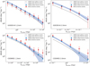 |
Fig. 7 Comparison between the differential number counts from simulations and observations at 1.2 mm (left panels) and 2 mm (right panels) in GOODS-N (upper panels) and COSMOS (lower panels). The solid blue line represents the source number counts derived directly from SIDES noiseless maps (see Sect. 4.2), while the blue squares are the source number counts estimated using the full analysis pipeline (map making, source extraction, and statistical corrections). These are the input and output source number counts from the simulation. The blue shaded area illustrates the 1σ field-to-field variance of the output source number counts. As several galaxies can contribute to a source, we also show the galaxy number counts in SIDES as the black dashed line in the figure (see discussion in Sect. 4.3). Finally, the number counts measured from N2CLS are represented by red diamonds. |
Combined differential and cumulative galaxy number counts at 1.2 and 2 mm from the observation on the two fields.
4.4.3 Comparison with other 2 mm number counts measurements
In recent decades, only a few blind surveys at around 2 mm have been carried out. Two surveys were performed using the Goddard IRAM Superconducting mm Observer (GISMO) camera at the focus of the IRAM 30m telescope in the GOODS-N (31 arcmin2; Staguhn et al. 2014) and COSMOS (250 arcmin2; Magnelli et al. 2019). As they were carried out with the same telescope, these single-dish data have a similar beam size, and the source counts can be compared directly. Two ALMA surveys also determined the number counts: the MORA 2 mm survey, which mostly overlaps with the CANDELS stripe in COSMOS (184 arcmin2; Zavala et al. 2021), and the ALMACAL archival survey, which is based on ALMA calibrator observations (157 arcmin2; Chen et al. 2023). These two interferometric surveys have a subarcsecond resolution, and we can assume that they directly measure the galaxy number counts.
In the bottom panels of Fig. 8, we show a comparison between the number counts from these surveys and N2CLS. Our new N2CLS measurements agree with previous GISMO GOODS-N measurements from Staguhn et al. (2014). The N2CLS probes slightly fainter fluxes, and shows similar error bars for GOODS-N at faint fluxes, which may seem surprising considering our approximately five-times-larger survey area. This could be explained by our propagation of the flux deboosting uncertainties to the final error bars. There is a mild systematic offset (<2σ) between the COSMOS number counts from GISMO (Magnelli et al. 2019) and NIKA2. Our survey covers a 4.4 times larger area, and we cannot rule out the possibility that the area used by the GISMO study is not representative of the full field, as suggested by the absence of sources in the eastern part of their map. Unfortunately, our fields only partially overlap with the GISMO survey, preventing a direct comparison between the two measurements of the counts in the exact same region.
As explained in Sect. 4.3, the galaxy number counts measured by interferometers cannot be directly compared with source counts from single-dish surveys. Before comparing ALMA observations with N2CLS, we applied a corrective factor to our number counts and (Rdiff and Rcum, see Sect. 4.3). The galaxy number counts obtained after these corrections (orange and red solid lines in Fig. 8) agree very well with the ALMA data, highlighting the importance of taking into account resolution effects in the (sub-)mm. We can also note that N2CLS is deeper and covers a larger area than the MORA survey, demonstrating the efficiency of single-dish telescopes in performing wide and deep mm surveys.
Overall, our measurements agree with the literature, except for a mild tension with GISMO (Magnelli et al. 2019) measurements. Thanks to the mapping speed of the NIKA2 camera, our survey covers the full range explored by the previous surveys in a homogeneous way.
4.5 Comparison with models
We also compared our new measurements with number count predictions from various models of galaxy evolution, including both semi-empirical (Béthermin et al. 2017; Schreiber et al. 2017; Popping et al. 2020) and semi-analytical (Lagos et al. 2020) models.
The Simulated Infrared Dusty Extragalactic Sky (SIDES, Béthermin et al. 2017) and the Empirical Galaxy Generator (EGG; Schreiber et al. 2017) start from the stellar mass function and the evolution of the star-forming main sequence from observations to predict infrared and (sub-)mm fluxes; they also separately account for the emission of main sequence and star-bursts galaxies using different SED templates, both evolving with redshift. The semi-empirical model of Popping et al. (2020) assigns star formation rates in dark matter halos following the SFR-halo relation from the UNIVERSEMACHINE (Behroozi et al. 2019), and then uses empirical relations to estimate the dust mass and obscured star formation to predict the mm fluxes. The predictions of these latter authors are converted from 1.1 to 1.2 mm using the method explained in Sect. 4.4.2.
The SHARK semi-analytical model is introduced in Lagos et al. (2018). This type of model applies semi-analytical recipes to model the evolution of galaxies in dark-matter halos from numerical simulations. The dust emission and (sub-)mm fluxes of galaxies are then predicted based on their gas content and metallicity using a framework described in Lagos et al. (2019, 2020). As the original number counts of Lagos et al. (2018) are cumulative, we differentiated their curves to obtain the differential ones.
In Fig. 9, we show a comparison between model predictions and our N2CLS results. As most models are predicting galaxy rather than source number counts, we use the combined galaxy number counts from our two fields derived in Sect. 4.3. At 1.2 mm, the three semi-empirical models (SIDES, EGG, and Popping et al. 2020) agree at the 1 σ level with our observations at the faint end (<1.5 mJy), but tend to be systematically lower at the bright end (>1.5 mJy, ~1.5 σ for SIDES, up to 3 σ for EGG and Popping et al. 2020). In contrast, the SHARK semi-analytical model is compatible at the bright end, but has a systematic 1.5 σ excess at the faint end. A similar behavior is observed at 2 mm. However, because of the larger uncertainties on the measurements, SIDES and SHARK remain compatible with our observations at ~1 σ. The EGG model remains significantly under-predicted at the bright end (>0.6 mJy). This difference in behavior between semi-empirical and semi-analytical models is discussed in Sect. 5.
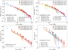 |
Fig. 8 Comparison between N2CLS GOODS-N (orange diamonds) and COSMOS (red diamonds) source number counts at 1.2 mm (top panels) and 2 mm (bottom panels). Differential and cumulative number counts are presented in the left and right panels, respectively. In each panel, the N2CLS galaxy number counts (see Sect. 4.3) and the corresponding 1 σ confidence interval are represented using red (COSMOS) and orange (GOODS-N) solid lines and shaded regions. All results from interferometric observations at 1.1 or 1.2 mm (Fujimoto et al. 2016, 2023; Hatsukade et al. 2016, 2018; Umehata et al. 2017; González-López et al. 2020; Gómez-Guijarro et al. 2022a; Chen et al. 2023) and 2 mm (Zavala et al. 2021; Chen et al. 2023) are shown as open circles. The measurements from single-dish observations at 1.1 or 1.2 mm (Lindner et al. 2011; Scott et al. 2012) and 2 mm (Staguhn et al. 2014; Magnelli et al. 2019) are represented by filled squares. |
5 Discussion
5.1 Modeling the mm number counts
As shown in Sect. 4.5, recent models are all able to reproduce the main trend of the mm number counts. The tension between models and observations remains small. This suggests that minor adjustments may be sufficient to reach a full agreement. Considering how challenging the (sub-)mm number counts have been for semi-analytical models and hydrodynamical simulations over the last two decades (e.g., Baugh et al. 2005; Hayward et al. 2013, 2021; Cousin et al. 2015; Somerville & Davé 2015; Narayanan et al. 2015; Lacey et al. 2016), this highlights the impressive progress made over recent years. The small residual tension between SHARK (Lagos et al. 2020) and observations at the faint end (<1.5 mJy) could be solved by fine tuning the star formation or feedback recipes. However, considering the large number of degrees of freedom in this type of model, it is hard to predict which exact change is the most relevant.
Semi-empirical models are more flexible, and updated models are often proposed shortly after the delivery of new observational constraints (e.g., Chary & Elbaz 2001; Franceschini et al. 2001; Lagache et al. 2004; Béthermin et al. 2011; Lapi et al. 2011; Gruppioni et al. 2013; Casey et al. 2018). These updates showed that modifications to the evolution of dusty galaxy populations or of their SEDs were necessary. The three recent semi-empirical models discussed in Sect. 4.5 are all slightly lower than our measured number counts at the bright end (>1.5 mJy). This systematic trend may suggest a common problem. The EGG (Schreiber et al. 2017) and Popping et al. (2020) models do not include the effect of strong lensing on the number counts (e.g., Negrello et al. 2010). This explains why these two models are lower than the SIDES model (Béthermin et al. 2017) in this regime, because 3%, 10%, and 60% of sources above 1.5 mJy, 3 mJy, and 5 mJy, respectively, are strongly lensed in SIDES.
However, even taking into account the lensing, SIDES number counts remain marginally low at the bright end (> 1.5 mJy). The two most simple explanations are a lack of galaxies with cold dust SEDs leading to fainter mm fluxes, and a small deficit of galaxies with high SFR (SFR ≳ 500 M⊙ yr−1). For instance, the fraction of starbursts in SIDES is fixed to 3% at z > 1 regardless of the stellar mass. A slightly higher fraction of star-bursts at high mass could be sufficient to match the observations, but hydrodynamical simulations find that high-z major mergers may be less efficient in enhancing star formation (Fensch et al. 2017). In addition, the SIDES model has a sharp SFR limit of 1000 M⊙ yr−1. This limit was motivated by the ALMA follow-up of bright mm sources, which showed that they were breaking into several components (Karim et al. 2013). However, a smoother cut allowing rare SFR > 1000 M⊙ yr−1 objects could reduce the tension with the observations.
Finally, the mm number counts are very sensitive to the assumptions on the far-IR SEDs. The SED templates used by SIDES (Béthermin et al. 2015a) and EGG (Schreiber et al. 2018) were calibrated using the observed mean evolution of the dust temperature up to z > 4, and are compatible with most of the recent ALMA results (Béthermin et al. 2020; Faisst et al. 2020; Sommovigo et al. 2022). A recent stacking-based analysis from Viero et al. (2022) suggests even higher dust temperatures, which would lead to an even greater disagreement between observed counts and empirical models. In contrast, recent studies also discovered DSFGs with far-IR SEDs peaking at a significantly longer wavelength than those of normal star-forming galaxies (e.g., Jin et al. 2019). At a fixed star formation rate, sources with these apparently cold-dust SEDs have higher mm fluxes. In any case, a larger scatter in the dust properties would naturally lead to higher number counts at the bright end. Extensive follow-up campaigns of mm sources with well-controlled selection biases might be the key to properly calibrating the SEDs in the models.
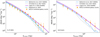 |
Fig. 9 Comparison between the N2CLS differential galaxy number counts (both fields combined, see Sect. 4.3) and the predictions from semi-empirical (Béthermin et al. 2017; Schreiber et al. 2017; Popping et al. 2020) and semi-analytical (Lagos et al. 2020) models. |
5.2 A framework for accurate interpretation of single-dish mm data
We highlighted the difference between the number density of sources viewed by high-angular-resolution interferometric observations and low-resolution (~15″) single-dish observations in the mm. The impact of angular resolution on flux measurements in single-dish observations has been discussed in interferometric follow up (e.g., Karim et al. 2013; Simpson et al. 2020) and modeling papers (e.g., Hayward et al. 2013; Scudder et al. 2016; Béthermin et al. 2017). Our work, for the first time, quantitatively estimates and corrects this effect for a single-dish blind survey. As shown in Sect. 4.3, the differences between the galaxy number counts and source number counts can reach a factor of two at 2 mm, even with a 30 m telescope. Correcting for this effect (Sect. 4.4), we show that interferometric and single-dish observations are fully consistent. Our paper proposes a new framework with which to interpret single-dish number counts without requiring systematic follow-up observations, and which can be applied to future surveys (e.g., Wilson et al. 2020; Klaassen et al. 2020; Ramasawmy et al. 2022).
5.3 Modeling the number of sources detected only at 2 mm
In Sect. 3.2, we find that a large fraction of the N2CLS sources is detected only at 2 mm (when considering S/N thresholds corresponding to 80% purity). This could suggest a large population of galaxies at very high redshifts. In contrast, in the SIDES input catalog, we find only an average of less than one source per field in GOODS-N and COSMOS, respectively, which are below the survey flux limit at 1.2 mm and above it at 2 mm. This corresponds to S1.2 mm<0.4 mJy and S2.0 mm>0.1 mJy in GOODS-N, and S1.2 mm<1.7 mJy and S2.0 mm>0.5 mJy in COSMOS. The observations seem to disagree strongly with the SIDES model. However, the instrument noise can be responsible for these sources. For instance, a source intrinsically just above the detection limit in both bands will be detected only at 2 mm if it coincides with a negative fluctuation of the noise at 1.2 mm. A similar phenomenon has already been identified for red Herschel/SPIRE sources (Béthermin et al. 2017; Donevski et al. 2018).
We used the 117 end-to-end simulations of each field presented in Sect. 4.2 to investigate the nature of these 2 mm-only sources. We find an average of 34 and 25 sources per field in GOODS-N and COSMOS, respectively (high-quality region only; see red contours in Figs. 1 and 2). Assuming Poisson uncertainties, this is compatible at 2 σ with the 23 and 27 sources detected in the real data (Sect. 3.2). In both fields, 87% of these sources are associated with a counterpart in the blob catalog. Most of these 2 mm detections are therefore associated with objects present in the simulation, and are not pure noise artifacts. This suggests that the combination of instrument noise, data reduction pipeline, and source extraction procedures could produce this apparent excess of 2 mm-only sources.
We checked whether or not an increase in the S/N threshold improves the situation. For an S/N threshold corresponding to 95% purity, we have 2 and 11 sources in the real GOODS-N and COSMOS catalogs, while the end-to-end simulations contain on average 6 and 8 sources per field. More than 98% of these sources are associated with an object in the blob catalog. However, there is still a mismatch with the input catalog in which less than one source per field is detected. This is not surprising given that we increased both 1.2 and 2 mm S/N thresholds and the mechanism producing spurious 2 mm-only detections still applies.
As shown by our simulations, the selection of sources detected only at 2 mm by NIKA2 is not a reliable way to select very high-redshift candidates. This also highlights the importance of end-to-end simulations in properly comparing models with observations.
6 Conclusion
We present the first results of the NIKA2 Cosmological Legacy Survey (N2CLS), a large blind mm survey in the GOODS-N and COSMOS fields with the NIKA2 camera on the IRAM 30 m telescope. We used the NIKA2 observations from October 2017 to May 2021, representing 86.15 h and 84.7 h on GOODS-N and COSMOS fields, respectively. The area used in our analysis is 159 arcmin2 for GOODS-N and 1010 arcmin2 for COSMOS. The survey reaches an unprecedented combination of depth and sky coverage at 1.2 and 2 mm. The main steps of our analysis and our main results are summarized below:
We built the maps using the IRAM PIIC software (Zylka 2013), and extracted the sources using our custom nikamap (Beelen 2023) package based on Astropy (Astropy Collaboration 2013, 2018, 2022) and Photutils (Bradley et al. 2022);
To characterize the performance of our analysis pipeline, we performed 117 end-to-end simulations of each field based on the SIDES model of galaxy evolution (Béthermin et al. 2017; Gkogkou et al. 2023). Here, we took advantage of the simulation mode of the PIIC pipeline, which accepts SIDES maps as input models to be injected into real NIKA2 timeline data. A half-difference method was applied to these timelines to remove only the true astrophysical signal but not the injected one. Maps and catalogs from the simulations were then produced following the data reduction and source detection procedures identical to that applied to N2CLS data and maps;
We then compared the output source catalogs of these end-to-end simulations with the input ones to determine the performance of our source-extraction algorithm. Because of the angular resolution of NIKA2, for the input catalogs, we use the blobs extracted from the noiseless maps rather than the individual galaxies. For each field and wavelength, we determined the sample purity as a function of the S/N threshold, and the completeness as a function of the source flux and the local noise level. With the S/N thresholds of 80% purity, we detect 120 and 195 sources at 1.2 mm in GOODS-N and COSMOS, respectively, and 67 and 76 sources at 2 mm. In the 1.2 mm maps of GOODS-N and COSMOS, we detect sources as faint as 0.4 mJy and 1.7 mJy in uncorrected PSF fluxes. At 2 mm, we reach limiting uncorrected PSF fluxes of 0.1 mJy and 0.5 mJy in GOODS-N and COSMOS, respectively;
We also computed the ratio between the output (measured) and the input (simulated) flux densities, taking into account the effects of both data reduction (flux filtering) and source extraction (flux boosting). The measured flux densities are on average lower than the input ones in GOODS-N, demonstrating that some flux is lost during the map-making and providing us with the corrections to apply;
We then computed the source number counts after correcting for all the effects listed above. We checked using our end-to-end simulations that our method is accurate. In addition, we derived the correction to convert our source number counts into galaxy number counts. This correction is necessary to compare our results with ALMA measurements and with models;
At 1.2 mm, our measurements cover the full flux density range from previous single-dish surveys and go a factor of 2 deeper, reaching the sub-mJy regime. We homogeneously probe 1.5 orders of magnitude in flux density and connect the bright single-dish number counts to the deep interferometric number counts. Our new measurements agree well with previous measurements after taking into account the resolution effects;
At 2 mm, our measurements match the depth of the deepest interferometric number counts and extend a factor of 2 above the brightest constraints. Our results agree with the single-dish measurements from Staguhn et al. (2014), and also with the interferometric constraints from Zavala et al. (2014) and Chen et al. (2023) after correcting for resolution effects. Results from Magnelli et al. (2019) are systematically ~1σ lower than our measurements;
Finally, we compared our measured galaxy number counts with a selection of recent semi-empirical (Béthermin et al. 2017; Schreiber et al. 2017; Popping et al. 2020) and semi-analytical (Lagos et al. 2020) models. The semi-empirical models agree at low flux density (<1.5 mJy), but tend to under-predict the counts at bright flux density (> 1.5 mJy). We discussed several possible causes such as the lack of strong lensing in some models, a deficit of high-SFR galaxies, and the dearth of objects with cold-dust SEDs. In contrast, the semi-analytical model of Lagos et al. (2020) over-predicts the counts at low flux while agreeing at higher flux.
The measurements and the models of mm source counts are now close to convergence. Stronger constraints will come from a full characterization of N2CLS sources and will allow us to test our models in greater detail. The upcoming follow-up observations with NOEMA/ALMA will pinpoint the location of galaxies contributing to the observed N2CLS flux. The rich ancillary data and ongoing JWST observations, such as COSMOS-Web (Casey et al. 2022), will help to identify the multiwavelength counterparts of N2CLS sources, construct their full SED, and determine their redshift distribution and physical properties. Thanks to its volume-complete flux selection, the N2CLS sample is an ideal reference sample with which to perform this full characterization of DSFGs.
We expect to reach a depth in COSMOS that is 1.5 times greater than that achieved here. The final COSMOS catalogs will be released together with the full COSMOS data release in a forthcoming paper. The identification and properties of sources with S/N > 4 in GOODS-N will be detailed in Berta et al. (in prep.) together with the complete source catalog. Also in GOODS-N, Ponthieu et al. (in prep.) will discuss the confusion noise due to distant galaxies for the IRAM 30m telescope.
Acknowledgements
The authors would like to thank the anonymous referee for the comments on the manuscript, as well as Gergö Popping and Claudia Lagos for providing their model prediction on mm number counts. L.B. warmly acknowledges financial support from IRAM for his first year of Ph.D Thesis and the support from the China Scholarship Council grant (CSC No. 201906190213). We acknowledge financial support from the “Programme National de Cosmologie and Galaxies” (PNCG) funded by CNRS/INSU-IN2P3-INP, CEA and CNES, France, from the European Research Council (ERC) under the European Union’s Horizon 2020 research and innovation programme (project CONCERTO, grant agreement No 788212) and from the Excellence Initiative of Aix-Marseille University-A*Midex, a French “Investissements d’Avenir” programme. This work is based on observations carried out under project numbers 192−16 with the IRAM 30 m telescope. IRAM is supported by INSU/CNRS (France), MPG (Germany) and IGN (Spain). We would like to thank the IRAM staff for their support during the campaigns. The NIKA2 dilution cryostat has been designed and built at the Institut Néel. In particular, we acknowledge the crucial contribution of the Cryogenics Group, and in particular Gregory Garde, Henri Rodenas, Jean-Paul Leggeri, Philippe Camus. This work has been partially funded by the Foundation Nanoscience Grenoble and the LabEx FOCUS ANR-11-LABX-0013. This work is supported by the French National Research Agency under the contracts “MKIDS”, “NIKA” and ANR-15-CE31-0017 and in the framework of the “Investissements d’avenir” program (ANR-15-IDEX-02). This work has benefited from the support of the European Research Council Advanced Grant ORISTARS under the European Union’s Seventh Framework Programme (Grant Agreement no. 291294). E.A. acknowledges funding from the French Programme d’investissements d’avenir through the Enigmass Labex. A.R. acknowledges financial support from the Italian Ministry of University and Research – Project Proposal CIR01_00010. The NIKA2 data were processed using the Pointing and Imaging In Continuum (PIIC) software, developed by Robert Zylka at the Institut de Radioastronomie Millimetrique (IRAM) and distributed by IRAM via the GILDAS pages. PIIC is the extension of the MOPSIC data reduction software to the case of NIKA2 data. This work made use of Astropy, a community-developed core Python package and an ecosystem of tools and resources for astronomy (Astropy Collaboration 2013, 2018, 2022). This research made use of Photutils, an Astropy package for detection and photometry of astronomical sources (Bradley et al. 2022).
Appendix A N2CLS 1.2 and 2 mm signal maps
The 1.2 mm and 2.0 mm signal maps from N2CLS GOODS-N and COSMOS observations are presented in Fig. A.1, Fig. A.2 and Fig. A.3
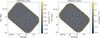 |
Fig. A.1 The 1.2 mm and 2 mm signal map from N2CLS GOODS-N observations. The high-quality region considered in N2CLS number counts analysis is enclosed by the red contour, which is defined in Sect. 2.2. |
References
- Adam, R., Comis, B., Macías-Pérez, J. F., et al. 2015, A&A, 576, A12 [NASA ADS] [CrossRef] [EDP Sciences] [Google Scholar]
- Adam, R., Adane, A., Ade, P. A. R., et al. 2018, A&A, 609, A115 [NASA ADS] [CrossRef] [EDP Sciences] [Google Scholar]
- Aravena, M., Decarii, R., Walter, F., et al. 2016, ApJ, 833, 68 [NASA ADS] [CrossRef] [Google Scholar]
- Aretxaga, I., Wilson, G. W., Aguilar, E., et al. 2011, MNRAS, 415, 3831 [Google Scholar]
- Arrabal Haro, P., Rodríguez Espinosa, J. M., Muñoz-Tuñón, C., et al. 2018, MNRAS, 478, 3740 [NASA ADS] [CrossRef] [Google Scholar]
- Astropy Collaboration (Robitaille, T. P., et al.) 2013, A&A, 558, A33 [NASA ADS] [CrossRef] [EDP Sciences] [Google Scholar]
- Astropy Collaboration (Price-Whelan, A. M., et al.) 2018, AJ, 156, 123 [Google Scholar]
- Astropy Collaboration (Price-Whelan, A. M., et al.) 2022, ApJ, 935, 167 [NASA ADS] [CrossRef] [Google Scholar]
- Barger, A. J., Cowie, L. L., Sanders, D. B., et al. 1998, Nature, 394, 248 [Google Scholar]
- Baugh, C. M., Lacey, C. G., Frenk, C. S., et al. 2005, MNRAS, 356, 1191 [Google Scholar]
- Beelen, A. 2023, https://zenodo.org/record/7520530 [Google Scholar]
- Behroozi, P., Wechsler, R. H., Hearin, A. P., & Conroy, C. 2019, MNRAS, 488, 3143 [NASA ADS] [CrossRef] [Google Scholar]
- Bertoldi, F., Carilli, C., Aravena, M., et al. 2007, ApJS, 172, 132 [Google Scholar]
- Béthermin, M., Dole, H., Lagache, G., Le Borgne, D., & Penin, A. 2011, A&A, 529, A4 [Google Scholar]
- Béthermin, M., Daddi, E., Magdis, G., et al. 2012, ApJ, 757, L23 [Google Scholar]
- Béthermin, M., Daddi, E., Magdis, G., et al. 2015a, A&A, 573, A113 [Google Scholar]
- Béthermin, M., De Breuck, C., Sargent, M., & Daddi, E. 2015b, A&A, 576, A9 [NASA ADS] [CrossRef] [EDP Sciences] [Google Scholar]
- Béthermin, M., Wu, H.-Y., Lagache, G., et al. 2017, A&A, 607, A89 [Google Scholar]
- Béthermin, M., Fudamoto, Y., Ginolfi, M., et al. 2020, A&A, 643, A2 [Google Scholar]
- Béthermin, M., Gkogkou, A., Van Cuyck, M., et al. 2022, A&A, 667, A156 [NASA ADS] [CrossRef] [EDP Sciences] [Google Scholar]
- Blain, A. W., Smail, I., Ivison, R. J., Kneib, J. P., & Frayer, D. T. 2002, Phys. Rep., 369, 111 [Google Scholar]
- Bourrion, O., Benoit, A., Bouly, J. L., et al. 2016, J. Instrum., 11, P11001 [Google Scholar]
- Bouwens, R. J., Smit, R., Schouws, S., et al. 2022, ApJ, 931, 160 [NASA ADS] [CrossRef] [Google Scholar]
- Bradley, L., Sipőcz, B., Robitaille, T., et al. 2022, https://zenodo.org/record/6825092 [Google Scholar]
- Brisbin, D., Miettinen, O., Aravena, M., et al. 2017, A&A, 608, A15 [NASA ADS] [CrossRef] [EDP Sciences] [Google Scholar]
- Calvo, M., Benoît, A., Catalano, A., et al. 2016, J. Low Temp. Phys., 184, 816 [CrossRef] [Google Scholar]
- Calvi, R., Dannerbauer, H., Arrabal Haro, P., et al. 2021, MNRAS, 502, 4558 [NASA ADS] [CrossRef] [Google Scholar]
- Capak, P. L., Carilli, C., Jones, G., et al. 2015, Nature, 522, 455 [NASA ADS] [CrossRef] [Google Scholar]
- Casey, C. M., Narayanan, D., & Cooray, A. 2014, Phys. Rep., 541, 45 [Google Scholar]
- Casey, C. M., Zavala, J. A., Spilker, J., et al. 2018, ApJ, 862, 77 [Google Scholar]
- Casey, C. M., Kartaltepe, J. S., Drakos, N. E., et al. 2022, ApJ, submitted [arXiv:2211.07865] [Google Scholar]
- Chapman, S. C., Blain, A. W., Smail, I., & Ivison, R. J. 2005, ApJ, 622, 772 [NASA ADS] [CrossRef] [Google Scholar]
- Chary, R., & Elbaz, D. 2001, ApJ, 556, 562 [Google Scholar]
- Chen, J., Ivison, R. J., Zwaan, M. A., et al. 2023, MNRAS, 518, 1378 [Google Scholar]
- Coppin, K., Halpern, M., Scott, D., Borys, C., & Chapman, S. 2005, MNRAS, 357, 1022 [NASA ADS] [CrossRef] [Google Scholar]
- Cousin, M., Lagache, G., Bethermin, M., Blaizot, J., & Guiderdoni, B. 2015, A&A, 575, A32 [NASA ADS] [CrossRef] [EDP Sciences] [Google Scholar]
- Cowie, L. L., Barger, A. J., Hsu, L. Y., et al. 2017, ApJ, 837, 139 [Google Scholar]
- Cowley, W. I., Lacey, C. G., Baugh, C. M., & Cole, S. 2015, MNRAS, 446, 1784 [Google Scholar]
- Daddi, E., Dannerbauer, H., Stern, D., et al. 2009, ApJ, 694, 1517 [Google Scholar]
- Donevski, D., Buat, V., Boone, F., et al. 2018, A&A, 614, A33 [NASA ADS] [CrossRef] [EDP Sciences] [Google Scholar]
- Dudzevičiūte, U., Smail, I., Swinbank, A. M., et al. 2020, MNRAS, 494, 3828 [NASA ADS] [CrossRef] [Google Scholar]
- Faisst, A. L., Fudamoto, Y., Oesch, P. A., et al. 2020, MNRAS, 498, 4192 [NASA ADS] [CrossRef] [Google Scholar]
- Fensch, J., Renaud, F., Bournaud, F., et al. 2017, MNRAS, 465, 1934 [NASA ADS] [CrossRef] [Google Scholar]
- Franceschini, A., Aussel, H., Cesarsky, C. J., Elbaz, D., & Fadda, D. 2001, A&A, 378, 1 [NASA ADS] [CrossRef] [EDP Sciences] [Google Scholar]
- Franco, M., Elbaz, D., Béthermin, M., et al. 2018, A&A, 620, A152 [NASA ADS] [CrossRef] [EDP Sciences] [Google Scholar]
- Fudamoto, Y., Oesch, P. A., Schouws, S., et al. 2021, Nature, 597, 489 [CrossRef] [Google Scholar]
- Fujimoto, S., Ouchi, M., Ono, Y., et al. 2016, ApJS, 222, 1 [Google Scholar]
- Fujimoto, S., Kohno, K., Ouchi, M., et al. 2023, ApJS, submitted [arXiv:2303.01658] [Google Scholar]
- Geach, J. E., Dunlop, J. S., Halpern, M., et al. 2017, MNRAS, 465, 1789 [Google Scholar]
- Gkogkou, A., Béthermin, M., Lagache, G., et al. 2023, A&A, 670, A16 [NASA ADS] [CrossRef] [EDP Sciences] [Google Scholar]
- Gómez-Guijarro, C., Elbaz, D., Xiao, M., et al. 2022a, A&A, 658, A43 [NASA ADS] [CrossRef] [EDP Sciences] [Google Scholar]
- Gómez-Guijarro, C., Elbaz, D., Xiao, M., et al. 2022b, A&A, 659, A196 [NASA ADS] [CrossRef] [EDP Sciences] [Google Scholar]
- González-López, J., Novak, M., Decarli, R., et al. 2020, ApJ, 897, 91 [Google Scholar]
- Gruppioni, C., Pozzi, F., Rodighiero, G., et al. 2013, MNRAS, 432, 23 [Google Scholar]
- Gruppioni, C., Béthermin, M., Loiacono, F., et al. 2020, A&A, 643, A8 [NASA ADS] [CrossRef] [EDP Sciences] [Google Scholar]
- Hatsukade, B., Kohno, K., Umehata, H., et al. 2016, PASJ, 68, 36 [NASA ADS] [CrossRef] [Google Scholar]
- Hatsukade, B., Kohno, K., Yamaguchi, Y., et al. 2018, PASJ, 70, 105 [Google Scholar]
- Hayward, C. C., Narayanan, D., Kereš, D., et al. 2013, MNRAS, 428, 2529 [Google Scholar]
- Hayward, C. C., Sparre, M., Chapman, S. C., et al. 2021, MNRAS, 502, 2922 [Google Scholar]
- Hodge, J. A., & da Cunha, E. 2020, Roy. Soc. Open Sci., 7, 200556 [NASA ADS] [CrossRef] [Google Scholar]
- Hodge, J. A., Karim, A., Smail, I., et al. 2013, ApJ, 768, 91 [Google Scholar]
- Ishiyama, T., Prada, F., Klypin, A. A., et al. 2021, MNRAS, 506, 4210 [NASA ADS] [CrossRef] [Google Scholar]
- Ivison, R. J., Greve, T. R., Dunlop, J. S., et al. 2007, MNRAS, 380, 199 [Google Scholar]
- Jin, S., Daddi, E., Magdis, G. E., et al. 2019, ApJ, 887, 144 [Google Scholar]
- Karim, A., Swinbank, A. M., Hodge, J. A., et al. 2013, MNRAS, 432, 2 [Google Scholar]
- Klaassen, P. D., Mroczkowski, T. K., Cicone, C., et al. 2020, SPIE Conf. Ser., 11445, 114452F [NASA ADS] [Google Scholar]
- Lacey, C. G., Baugh, C. M., Frenk, C. S., et al. 2016, MNRAS, 462, 3854 [Google Scholar]
- Lagache, G., Dole, H., Puget, J. L., et al. 2004, ApJS, 154, 112 [NASA ADS] [CrossRef] [Google Scholar]
- Lagache, G., Puget, J.-L., & Dole, H. 2005, ARA&A, 43, 727 [NASA ADS] [CrossRef] [Google Scholar]
- Lagos, C. D. P., Tobar, R. J., Robotham, A. S. G., et al. 2018, MNRAS, 481, 3573 [CrossRef] [Google Scholar]
- Lagos, C. D. P., Robotham, A. S. G., Trayford, J. W., et al. 2019, MNRAS, 489, 4196 [NASA ADS] [CrossRef] [Google Scholar]
- Lagos, C. D. P., da Cunha, E., Robotham, A. S. G., et al. 2020, MNRAS, 499, 1948 [CrossRef] [Google Scholar]
- Lapi, A., González-Nuevo, J., Fan, L., et al. 2011, ApJ, 742, 24 [NASA ADS] [CrossRef] [Google Scholar]
- Liang, L., Feldmann, R., Faucher-Giguère, C.-A., et al. 2018, MNRAS, 478, L83 [Google Scholar]
- Lindner, R. R., Baker, A. J., Omont, A., et al. 2011, ApJ, 737, 83 [NASA ADS] [CrossRef] [Google Scholar]
- Liu, D., Daddi, E., Dickinson, M., et al. 2018, ApJ, 853, 172 [Google Scholar]
- Lovell, C. C., Geach, J. E., Davé, R., Narayanan, D., & Li, Q. 2021, MNRAS, 502, 772 [NASA ADS] [CrossRef] [Google Scholar]
- Madau, P., & Dickinson, M. 2014, ARA&A, 52, 415 [Google Scholar]
- Magnelli, B., Karim, A., Staguhn, J., et al. 2019, ApJ, 877, 45 [NASA ADS] [CrossRef] [Google Scholar]
- McAlpine, S., Smail, I., Bower, R. G., et al. 2019, MNRAS, 488, 2440 [NASA ADS] [CrossRef] [Google Scholar]
- Monfardini, A., Adam, R., Adane, A., et al. 2014, J. Low Temp. Phys., 176, 787 [NASA ADS] [CrossRef] [Google Scholar]
- Muñoz-Echeverría, M., Macías-Pérez, J. F., Pratt, G. W., et al. 2023, A&A, 671, A28 [NASA ADS] [CrossRef] [EDP Sciences] [Google Scholar]
- Narayanan, D., Turk, M., Feldmann, R., et al. 2015, Nature, 525, 496 [NASA ADS] [CrossRef] [Google Scholar]
- Negrello, M., Hopwood, R., De Zotti, G., et al. 2010, Science, 330, 800 [NASA ADS] [CrossRef] [Google Scholar]
- Oteo, I., Zwaan, M. A., Ivison, R. J., Smail, I., & Biggs, A. D. 2016, ApJ, 822, 36 [NASA ADS] [CrossRef] [Google Scholar]
- Perera, T. A., Chapin, E. L., Austermann, J. E., et al. 2008, MNRAS, 391, 1227 [NASA ADS] [CrossRef] [Google Scholar]
- Perotto, L., Ponthieu, N., Macías-Pérez, J. F., et al. 2020, A&A, 637, A71 [NASA ADS] [CrossRef] [EDP Sciences] [Google Scholar]
- Popping, G., Walter, F., Behroozi, P., et al. 2020, ApJ, 891, 135 [NASA ADS] [CrossRef] [Google Scholar]
- Ramasawmy, J., Klaassen, P. D., Cicone, C., et al. 2022, SPIE Conf. Ser., 12190, 1219007 [NASA ADS] [Google Scholar]
- Schreiber, C., Elbaz, D., Pannella, M., et al. 2017, A&A, 602, A96 [NASA ADS] [CrossRef] [EDP Sciences] [Google Scholar]
- Schreiber, C., Elbaz, D., Pannella, M., et al. 2018, A&A, 609, A30 [NASA ADS] [CrossRef] [EDP Sciences] [Google Scholar]
- Scott, K. S., Wilson, G. W., Aretxaga, I., et al. 2012, MNRAS, 423, 575 [NASA ADS] [CrossRef] [Google Scholar]
- Scudder, J. M., Oliver, S., Hurley, P. D., et al. 2016, MNRAS, 460, 1119 [NASA ADS] [CrossRef] [Google Scholar]
- Simpson, J. M., Smail, I., Swinbank, A. M., et al. 2019, ApJ, 880, 43 [NASA ADS] [CrossRef] [Google Scholar]
- Simpson, J. M., Smail, I., Dudzevičiūtė, U., et al. 2020, MNRAS, 495, 3409 [Google Scholar]
- Somerville, R. S., & Davé, R. 2015, ARA&A, 53, 51 [Google Scholar]
- Sommovigo, L., Ferrara, A., Carniani, S., et al. 2022, MNRAS, 517, 5930 [NASA ADS] [CrossRef] [Google Scholar]
- Spilker, J. S., Bezanson, R., Weiner, B. J., Whitaker, K. E., & Williams, C. C. 2019, ApJ, 883, 81 [NASA ADS] [CrossRef] [Google Scholar]
- Staguhn, J. G., Kovács, A., Arendt, R. G., et al. 2014, ApJ, 790, 77 [NASA ADS] [CrossRef] [Google Scholar]
- Strandet, M. L., Weiss, A., De Breuck, C., et al. 2017, ApJ, 842, L15 [Google Scholar]
- Toft, S., Smolcic, V., Magnelli, B., et al. 2014, ApJ, 782, 68 [NASA ADS] [CrossRef] [Google Scholar]
- Umehata, H., Tamura, Y., Kohno, K., et al. 2017, ApJ, 835, 98 [Google Scholar]
- Valentino, F., Magdis, G. E., Daddi, E., et al. 2020, ApJ, 890, 24 [Google Scholar]
- Venemans, B. P., Walter, F., Neeleman, M., et al. 2020, ApJ, 904, 130 [Google Scholar]
- Viero, M. P., Sun, G., Chung, D. T., Moncelsi, L., & Condon, S. S. 2022, MNRAS, 516, L30 [NASA ADS] [CrossRef] [Google Scholar]
- Walter, F., Decarli, R., Carilli, C., et al. 2012, Nature, 486, 233 [Google Scholar]
- Wilson, G. W., Abi-Saad, S., Ade, P., et al. 2020, SPIE Conf. Ser., 11453, 1145302 [NASA ADS] [Google Scholar]
- Zavala, J. A., Aretxaga, I., & Hughes, D. H. 2014, MNRAS, 443, 2384 [NASA ADS] [CrossRef] [Google Scholar]
- Zavala, J. A., Casey, C. M., Manning, S. M., et al. 2021, ApJ, 909, 165 [CrossRef] [Google Scholar]
- Zylka, R. 2013, Astrophysics Source Code Library [record ascl:1303.011] [Google Scholar]
Available at https://gitlab.lam.fr/N2CLS/nikamap
All Tables
Comparison of N2CLS-May21 depth to other single-dish (sub)mm surveys in GOODS-N and COSMOS, which are all given as 1σ of the noise level.
Differential and cumulative source number counts at 1.2 mm in GOODS-N and COSMOS.
Combined differential and cumulative galaxy number counts at 1.2 and 2 mm from the observation on the two fields.
All Figures
|
Fig. 1 Maps of signal-to-noise ratio (left panels) and noise (σinst in mJy/beam, right panels) of the 1.2 mm N2CLS maps of the GOODS-N (upper panels) and COSMOS (lower panels) fields. The S/N maps and noise maps are matched filtered (see Sect. 2.3). The regions enclosed in the red contours (159 arcmin2 for GOODS-N and 1010 arcmin2 for COSMOS) have sufficiently low noise to be analyzed by our source-detection algorithm, and our catalogs and number counts are derived only in these areas (see Sects. 2.3 and 4). |
| In the text | |
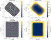 |
Fig. 2 Same as Fig. 1 but at 2 mm. |
| In the text | |
|
Fig. 3 Pixel S/N distribution within the high-quality regions of the 1.2 and 2 mm maps shown in Figs. 1 and 2, as well as the average distribution of pixel S/N in 100 randomly generated half-difference maps for each field and waveband (see Sect. 2.2). The red-shaded region illustrates the best-fit normal distribution on the average histograms of the half-difference maps. |
| In the text | |
|
Fig. 4 Purity of detected sources at different S/N in the matched-filter map from the simulations at 1.2 and 2 mm in the GOODS-N (top panels) and COSMOS (lower panels) fields. |
| In the text | |
|
Fig. 5 Ratio between the source fluxes measured in the output simulated maps (fout) and the source fluxes from the input blob catalog (ftrue) as functions of S/N at 1.2 mm (left panels) and 2 mm (right panels) in GOODS-N (upper panels) and COSMOS (lower panels). This corresponds to the effective flux boosting described in Sect. 3.3. The boxes shown for each S/N bin represent ranges between 25% and 75% of the cumulative distribution and the upper and lower bounds of error bars present 5% to 95% of the cumulative distribution (within 1σ). The width of each box corresponds to the width of the corresponding S/Ncorr bin. The red dotted line shows the position of unity effective flux boosting as a reference for each plot. In addition, we use color-coded solid-filled circles to present the median flux boosting in regions with different noise levels. |
| In the text | |
|
Fig. 6 Completeness of sources in N2CLS as a function of the ratio between source flux density and instrumental noise level (ftrue/σinst) at 1.2 mm (left panels) and 2 mm (right panels) in GOODS-N (upper panels) and COSMOS (lower panels). The completeness in various survey areas with different instrumental noise levels is presented as bluish color-coded dots, and the average completeness over the whole survey area is shown using oranges dots. The red line shows the best fit of the average completeness using the functional form of Eq. (3). |
| In the text | |
|
Fig. 7 Comparison between the differential number counts from simulations and observations at 1.2 mm (left panels) and 2 mm (right panels) in GOODS-N (upper panels) and COSMOS (lower panels). The solid blue line represents the source number counts derived directly from SIDES noiseless maps (see Sect. 4.2), while the blue squares are the source number counts estimated using the full analysis pipeline (map making, source extraction, and statistical corrections). These are the input and output source number counts from the simulation. The blue shaded area illustrates the 1σ field-to-field variance of the output source number counts. As several galaxies can contribute to a source, we also show the galaxy number counts in SIDES as the black dashed line in the figure (see discussion in Sect. 4.3). Finally, the number counts measured from N2CLS are represented by red diamonds. |
| In the text | |
|
Fig. 8 Comparison between N2CLS GOODS-N (orange diamonds) and COSMOS (red diamonds) source number counts at 1.2 mm (top panels) and 2 mm (bottom panels). Differential and cumulative number counts are presented in the left and right panels, respectively. In each panel, the N2CLS galaxy number counts (see Sect. 4.3) and the corresponding 1 σ confidence interval are represented using red (COSMOS) and orange (GOODS-N) solid lines and shaded regions. All results from interferometric observations at 1.1 or 1.2 mm (Fujimoto et al. 2016, 2023; Hatsukade et al. 2016, 2018; Umehata et al. 2017; González-López et al. 2020; Gómez-Guijarro et al. 2022a; Chen et al. 2023) and 2 mm (Zavala et al. 2021; Chen et al. 2023) are shown as open circles. The measurements from single-dish observations at 1.1 or 1.2 mm (Lindner et al. 2011; Scott et al. 2012) and 2 mm (Staguhn et al. 2014; Magnelli et al. 2019) are represented by filled squares. |
| In the text | |
|
Fig. 9 Comparison between the N2CLS differential galaxy number counts (both fields combined, see Sect. 4.3) and the predictions from semi-empirical (Béthermin et al. 2017; Schreiber et al. 2017; Popping et al. 2020) and semi-analytical (Lagos et al. 2020) models. |
| In the text | |
|
Fig. A.1 The 1.2 mm and 2 mm signal map from N2CLS GOODS-N observations. The high-quality region considered in N2CLS number counts analysis is enclosed by the red contour, which is defined in Sect. 2.2. |
| In the text | |
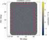 |
Fig. A.2 Same as Fig. A.1. but for N2CLS COSMOS 1.2 mm observations. |
| In the text | |
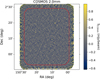 |
Fig. A.3 Same as Fig. A.1. but for N2CLS COSMOS 2 mm observations. |
| In the text | |
Current usage metrics show cumulative count of Article Views (full-text article views including HTML views, PDF and ePub downloads, according to the available data) and Abstracts Views on Vision4Press platform.
Data correspond to usage on the plateform after 2015. The current usage metrics is available 48-96 hours after online publication and is updated daily on week days.
Initial download of the metrics may take a while.