| Issue |
A&A
Volume 676, August 2023
|
|
|---|---|---|
| Article Number | A41 | |
| Number of page(s) | 15 | |
| Section | Extragalactic astronomy | |
| DOI | https://doi.org/10.1051/0004-6361/202346528 | |
| Published online | 04 August 2023 | |
Variation in optical and infrared properties of galaxies in relation to their surface brightness⋆
1
National Centre for Nuclear Research, Pasteura 7, 02-093 Warsaw, Poland
e-mail: This email address is being protected from spambots. You need JavaScript enabled to view it.
2
Aix-Marseille Univ., CNRS, CNES, LAM, Marseille, France
3
Department of Physics, National Tsing Hua University, 101, Section 2, Kuang-Fu Road, Hsinchu 30013, Taiwan, ROC
4
Institute of Astronomy, National Tsing Hua University, 101, Section 2, Kuang-Fu Road, Hsinchu 30013, Taiwan, ROC
5
Department of Physics and Astronomy, Stony Brook University, Stony Brook, NY 11794-3800, USA
6
Department of Space and Astronautical Science, The Graduate University for Advanced Studies, SOKENDAI, 3-1-1 Yoshinodai, Chuo-ku, Sagamihara, Kanagawa 252-5210, Japan
7
Institute of Space and Astronautical Science, Japan Aerospace Exploration Agency, 3-1-1 Yoshinodai, Chuo-ku, Sagamihara, Kanagawa 252-5210, Japan
8
INAF – Osservatorio Astronomico di Padova, Vicolo dell’Osservatorio 5, 35122 Padova, Italy
9
Centro de Astronomá (CITEVA), Universidad de Antofagasta, Avenida Angamos 601, Antofagasta, Chile
10
SISSA, Via Bonomea 265, 34136 Trieste, Italy
Received:
29
March
2023
Accepted:
9
June
2023
Abstract
Although it is now recognized that low surface brightness galaxies (LSBs) constitute a large fraction of the number density of galaxies, many of their properties are still poorly known. Based on only a few studies, LSBs are often considered to be “dust poor”, that is, with a very low amount of dust. For the first time, we use a large sample of LSBs and high surface brightness galaxies (HSBs) with deep observational data to study the variation of stellar and dust properties as a function of the surface brightness-surface mass density. Our sample consists of 1631 galaxies that were optically selected (with ugrizy-bands) at z < 0.1 from the North Ecliptic Pole (NEP) Wide field. We used the large multiwavelength set of ancillary data in this field ranging from UV to the far-infrared wavelengths. We measured the optical size and the surface brightness of the targets and analyzed their spectral energy distribution using the CIGALE fitting code. Based on the average r-band surface brightness (μ̄e), our sample consists of 1003 LSBs (μ̄e > 23 mag arcsec−2) and 628 HSBs (μ̄e ≤ 23 mag arcsec−2). We found that the specific star formation rate and specific infrared luminosity (total infrared luminosity per stellar mass) remain mostly flat as a function of surface brightness for both LSBs and HSBs that are star forming, but these characteristics decline steeply when the LSBs and HSBs are quiescent galaxies. The majority of LSBs in our sample have negligible dust attenuation (< 0.1 mag), and only about 4% of them show significant attenuation, with a mean V-band attenuation of 0.8 mag. We found that the LSBs with a significant attenuation also have a high r-band mass-to-light ratio (M/Lr > 3 M⊙/L⊙), making them outliers from the linear relation of surface brightness and stellar mass surface density. These outlier LSBs also show similarity to the extreme giant LSBs from the literature, indicating a possibly higher dust attenuation in giant LSBs. This work provides a large catalog of LSBs and HSBs as well as detailed measurements of several optical and infrared physical properties. Our results suggest that the dust content of LSBs is more varied than previously thought, with some of them having significant attenuation that makes them fainter than their intrinsic value. With these results, we will be able to make predictions on the dust content of the population of LSBs and how the presence of dust will affect their observations from current and upcoming surveys like JWST and LSST.
Key words: galaxies: general / galaxies: formation / galaxies: star formation / galaxies: ISM
Full Table B.1 is only available at the CDS via anonymous ftp to cdsarc.cds.unistra.fr (130.79.128.5) or via https://cdsarc.cds.unistra.fr/viz-bin/cat/J/A+A/676/A41
© The Authors 2023
 Open Access article, published by EDP Sciences, under the terms of the Creative Commons Attribution License (https://creativecommons.org/licenses/by/4.0), which permits unrestricted use, distribution, and reproduction in any medium, provided the original work is properly cited.
This article is published in open access under the Subscribe to Open model. This email address is being protected from spambots. You need JavaScript enabled to view it. to support open access publication.
1. Introduction
In recent years, advances in technology have allowed astronomers to study different types of galaxies in great detail, bringing new interest in low surface brightness galaxies (LSBs). To have a comprehensive view of galaxy evolution, we have to consider high surface brightness galaxies (HSBs) and LSBs. Galaxies characterized as HSBs are “typical” bright galaxies, and they have been well studied in the literature, but LSBs, which are much fainter, have only recently become more accessible for detailed studies.
Low surface brightness galaxies are generally defined as diffuse galaxies that are fainter than the typical night sky surface brightness level of ∼23 mag arcsec−2 in the B-band (Bothun et al. 1997). However, we note that there is no single definition for LSBs in the literature, and it varies among different works. Therefore, in this work, we consider LSBs as galaxies with an average r-band surface brightness  mag arcsec−2 and HSBs as galaxies with
  mag arcsec−2, following similar definitions adopted in previous works (e.g., Martin et al. 2019). Notably, LSBs span a wide range of sizes, masses, and morphologies, from the most massive giant low surface brightness galaxies down to more common dwarf systems (e.g., Sprayberry et al. 1995; Matthews et al. 2001; Junais et al. 2022). It has been estimated that LSBs make up a significant fraction of more than 50% of the total number density of galaxies in the universe (O’Neil & Bothun 2000; Blanton et al. 2005; Galaz et al. 2011; Martin et al. 2019), and about 10% of the baryonic mass budget (Minchin et al. 2004). Such an abundance of LSBs could steepen the faint-end slope of the galaxy stellar mass and luminosity function (Sabatini et al. 2003; Blanton et al. 2005; Sedgwick et al. 2019; Kim et al. 2023). Although LSBs are generally found to be gas rich, their gas surface densities are usually about a factor of three lower than that of HSBs (de Blok et al. 1996; Gerritsen & de Blok 1999). As star formation in galaxies is linked to gas surface density (Kennicutt & Evans 2012), this directly affects the ability of LSBs to form stars, resulting in LSBs having a low stellar mass surface density as well. Therefore, LSBs are a perfect laboratory for studying star formation activity in low-density regimes (Boissier et al. 2008; Wyder et al. 2009; Bigiel et al. 2010).
Due to the very low densities and low star formation, LSBs are also generally considered to have a very low amount of dust. Their low metallicities also imply that their dust-to-gas ratios should be lower than those of their HSB counterparts (Bell et al. 2000). Holwerda et al. (2005) showed that LSB disks are effectively transparent and are without any extinction where multiple distant galaxies were observed through their disks. Moreover, most of the observations of LSBs at infrared wavelengths have resulted in non-detections (Hinz et al. 2007; Rahman et al. 2007), indicating either a very weak or non-detectable dust emission.
Nevertheless, we cannot necessarily conclude that the entire population of LSBs, which consists of a wide range of galaxy types, is dust poor. Liang et al. (2010) found that LSBs selected from the Sloan Digital Sky Survey (SDSS) span a wide range in their dust attenuation, measured using the Balmer decrement (AV in the range of 0−1 mag with a median value of ∼0.4 mag). This indicates that not all LSBs are dust poor. However, since surveys like SDSS are very shallow and incomplete beyond  mag arcsec−2, only the brighter end of the LSB population can be observed by them, and they lack information about the remaining bulk of the faintest LSBs that are consequently missed (e.g., Kniazev et al. 2004; Williams et al. 2016). In another work, Cortese et al. (2012b) showed that the specific dust mass (dust to stellar mass ratio) of local galaxies from the Herschel Reference survey (HRS; Boselli et al. 2010) increases toward fainter galaxies. This yet again indicates that LSBs could have dust masses comparable with HSBs of similar stellar mass. It is likely that the dust in LSBs is distributed very diffusely, similar to their stellar population and gas content, making it extremely hard to detect (Hinz et al. 2008).
Currently, most studies on dust or infrared properties of LSBs have been done using either very small samples (e.g., Rahman et al. 2007; Hinz et al. 2007; Wyder et al. 2009) or shallow data (e.g., Liang et al. 2010), which may be not sufficient to make a general conclusion on the large population of LSBs. A large statistical sample of galaxies at different surface brightness levels is needed to properly understand how these properties change between LSBs and HSBs. In this work, we aim to do this by collecting a large sample of both LSBs and HSBs with deep data in order to constrain their optical and infrared properties and quantify how the presence of dust (if any) affects our observations of them. Such a work will be particularly significant in the context of current and upcoming observational facilities, such as the Large Synoptic Survey Telescope (LSST; Ivezić et al. 2019) and the James Webb Space Telescope (JWST; Gardner et al. 2006), where a large number of LSBs will be observed.
This paper is structured as follows: Section 2 describes the data and the sample used in this work. Section 2.2 introduces the comparison sample we use from the literature. Section 3 describes our spectral energy distribution fitting procedure. The results of our analysis are presented in Sect. 4, and a global discussion is given in Sect. 5. We conclude in Sect. 6.
Throughout this work, we adopt a Chabrier (2003) initial mass function (IMF) and a ΛCDM cosmology with H0 = 70 km s−1 Mpc−1, ΩM = 0.27, and ΩΛ = 0.73. All the magnitudes given in this paper are in the AB system.
2. Data and samples
2.1. Main sample
In this work, we use the large set of multiwavelength data ranging from UV to far-infrared (FIR) wavelengths available for the North Ecliptic Pole (NEP) Wide field, which covers an area of ∼5.4 deg2 (see Kim et al. 2021 for a detailed description of the available data). This also includes deep optical data from the Subaru Hyper Suprime-Cam (HSC; Oi et al. 2021) and the Canada-France-Hawaii Telescope (CFHT) Megcam/Megaprime1 (Huang et al. 2020), which is used as a basis for our sample selection (discussed in Sect. 2.1.1). The NEP Wide field has a very deep coverage in optical wavelengths, with a 5σ detection limit of 25.4, 28.6, 27.3, 26.7, 26.0, and 25.6 mag in the ugrizy-bands, respectively2. We note that this is very close to the 5σ depth of the upcoming LSST survey in similar bands (Bianco et al. 2022). In both cases, the depth of the data is suited to explore the properties of galaxies as a function of surface brightness, which is the goal of this work. Moreover, the NEP field is also well suited to the study of dust and attenuation within galaxies, due to the extensive coverage of this field in the infrared wavelengths (e.g., AKARI, WISE, Spitzer, Herschel; Kim et al. 2021) as well as very low foreground Galactic extinction along the line of sight of the NEP field.
2.1.1. Sample selection
Our sample was selected from the HSC grizy-bands and CFHT u-band data (Huang et al. 2020; Oi et al. 2021). Only the galaxies with a 5σ detection in all six of the associated bands were included in our sample. The u-band, with its short wavelength, is more sensitive toward dust attenuation. Therefore, the choice of including a u-band detection facilitates secure dust attenuation estimates for our sample, which we intend to do in this work. Moreover, a selection in the ugrizy also mimics the upcoming LSST observations in the same bands, where there will be a vast discovery space for LSBs.
We also applied an arbitrary selection in redshift in order to include only local galaxies with z < 0.1. We imposed this limit since we aim to study the properties of galaxies as a function of surface brightness, and the cosmological dimming would make us lose the LSBs at high-z. For this purpose, we use either the photometric redshifts provided by Huang et al. (2021) or the spectroscopic redshifts, when available (see Kim et al. 2021 for more details on the available spectroscopic data). The photometric redshifts from Huang et al. (2021) were computed with the Le Phare code (Arnouts et al. 1999; Ilbert et al. 2006) using the ugrizy-bands. Moreover, the Spitzer IRAC 1 (3.6 μm) and IRAC 2 (4.5 μm) bands were also included in the photometric redshift estimation, when available. The photometric redshifts attain an accuracy of σzp = 0.063 and a catastrophic outlier rate of 8.6% (Huang et al. 2021). With the above selection procedure based on optical detection and the redshift cut, our sample therefore contains 1950 galaxies. Among them, only 66 galaxies have spectroscopic redshifts.
We verified that a strict selection based on the ugrizy bands as discussed above does not introduce any bias toward bluer or redder galaxies in our sample. To perform this test, we looked at an alternate sample selection based only on the HSC grizy-bands in the same area as our u-band observations. Such a selection increased our sample size by around 190 galaxies (among them about 90 galaxies are LSBs), as the HSC grizy observations are two to three orders of magnitude deeper than the CFHT u-band. However, we found that such a sample has a very similar distribution of optical colors as our initial ugrizy-based sample (mean g − r color of 0.53 mag for both the samples). This indicates that the inclusion of the u-band does not introduce a bias in our selection. Therefore, we chose to continue with our initial ugrizy- and redshift-based sample of 1950 galaxies.
2.1.2. Morphological fitting
To obtain the effective surface brightness and radius of each galaxy, we performed a morphological fitting procedure using the AutoProf tool (Stone et al. 2021). This tool is efficient for capturing the full radial surface brightness light profile of a galaxy from its image using a non-parametric approach, unlike the parametric fitting tools like Galfit (Peng et al. 2002), which do not always capture the total light from a galaxy. The AutoProf tool is also well suited for low surface brightness science, as it can extract about two orders of magnitude fainter isophotes from an image than any other conventional tool (Stone et al. 2021).
The surface brightness profile extraction of our sample was done on the HSC r-band images. Although the g-band is the deepest among our sample, the choice of the r-band (which is the second deepest) is motivated by the fact that the r-band is a better tracer of the stellar mass distribution in galaxies than the g-band (Mahajan et al. 2018). Figure 1 shows an example of the surface brightness profile obtained for a galaxy. Similarly, we extracted the profiles for the majority of the galaxies in our sample (1743 out of 1950 galaxies). The remaining sources have either failed or flagged profile fits. Therefore, we excluded from our sample all the sources without a reliable morphological fit, which left 1743 galaxies. We integrated each surface brightness profile until its last measured radius to estimate the total light from each galaxy, the corresponding effective radius (half-light radius; Re), and the average surface brightness within the effective radius ( ). From Fig. 1, the radial surface brightness profiles we obtained using AutoProf are clearly shown to reach well beyond the effective radius of the galaxy to about four times Re and are also ∼2 mag arcsec−2 deeper than the typical sky level (a similar trend was found for our full sample), which is ideal to probe LSBs. The distribution of the r-band Re and
  for our full sample is given in Fig. 2. Our sample at this stage consisted of 1041 LSBs and 702 HSBs (although such a distinction is based on an arbitrary definition, as discussed in Sect. 1). The LSBs have a median
  and Re of 23.8 mag arcsec−2 and 1.9 kpc, respectively. Whereas the HSBs are brighter and slightly larger in size, with a median
  and Re of 22.2 mag arcsec−2 and 2.2 kpc, respectively. In terms of the redshift, both the LSBs and HSBs have a similar distribution, with a median value of about 0.08. The r-band absolute magnitudes (Mr) of the two subsamples show a clear difference, as the LSBs are fainter than the HSBs, as expected from their selection, with a median Mr of −15.9 mag and −17.9 mag, respectively.
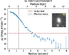 |
Fig. 1. Example of an r-band radial surface brightness profile extracted for a galaxy using AutoProf. The HSC r-band image of the galaxy is shown in the inset panel. The black dotted line marks the effective radius of the galaxy. The brown dashed horizontal line is the 1σ sky noise level. |
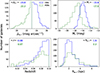 |
Fig. 2. Distribution of the basic properties of the LSBs (blue solid line) and HSBs (green dashed line) in our sample. The average r-band surface brightness within the effective radius and the r-band absolute magnitude are given in the top-left and top-right panels, respectively. The redshift and the effective radius are in the bottom-left and bottom-right panels, respectively. The median values corresponding to each parameter are marked inside each panel in blue and green for the LSBs and HSBs, respectively. |
We also made a comparison of our Re and  estimates with that of Pearson et al. (2022), who made a Sérsic profile fitting of the NEP galaxies in the same band using the statmorph tool (Rodriguez-Gomez et al. 2019). We found that, in general, our values are in agreement with Pearson et al. (2022), with a mean difference in Re of 0.01 ± 0.23 dex and −0.02 ± 0.76 mag arcsec−2 for the
  .
.
2.1.3. Crossmatching with multiwavelength catalogs
After the initial sample selection and their morphological fitting, we crossmatched our optically selected sample with all the available multiwavelength data on hand. For the NEP field, other than the optical data from HSC and CFHT, we had ancillary data available from GALEX (FUV and NUV bands; Bianchi et al. 2017); AKARI (N2, N3, N4, S7, S9W, S11, L15, L18W, and L24 bands; Kim et al. 2012); CFHT/WIRCam (Y, J, and Ks bands; Oi et al. 2014); KPNO/FLAMINGOS (J and H bands; Jeon et al. 2014); Spitzer/IRAC (band 1 and 2; Nayyeri et al. 2018); WISE (band 1 to 4; Jarrett et al. 2011); and Herschel PACS/SPIRE (100 μm, 160 μm, 250 μm, 350 μm and 500 μm bands; Pearson et al. 2017, 2019). A detailed description of the data is given in Kim et al. (2021). The multiband photometry obtained from the crossmatching of these catalogs was later used in the spectral energy distribution (SED) fitting procedure discussed in Sect. 3. The crossmatching was done following Kim et al. (2021), where a 3σ positional offset in the RA/Dec coordinates corresponding to each dataset with respect to the HSC coordinates were used as the crossmatching radii. For GALEX, AKARI, WIRCam, FLAMINGOS, IRAC, WISE, PACS, and SPIRE, we used a crossmatching radius of 1.5″, 1.5″, 0.5″, 0.65″, 0.58″, 0.7″, 2.75″, and 8.44″, respectively. Figure 3 shows the distribution of galaxies with counterparts in each dataset. About 62% of the galaxies in the sample (1086 out of 1743 sources) have at least one counterpart outside the ugrizy optical range.
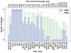 |
Fig. 3. Distribution of the multiwavelength data available for the sample. The LSBs and HSBs are marked as the blue striped bars and the green dashed bars, respectively. The broadband filter names and their corresponding wavelengths are given in the bottom and top horizontal axes, respectively. All the galaxies in the sample have detection in the ugrizy-bands. |
We also compared our sample with the band-merged catalog of Kim et al. (2021), who identified HSC counterparts for the AKARI-detected sources in NEP. Only 532 galaxies of our sample overlapped with the Kim et al. (2021) catalog, indicating that the rest of our sources do not have any AKARI counterparts in near-infrared or mid-infrared (MIR). Moreover, ∼85% of our sample does not have any detection in the MIR and FIR regime (in the 7 μm to 500 μm wavelength range), as shown in Fig. 3. However, since we aim to study the IR properties of our sample, it is crucial to have observational constraints in the MIR and FIR range. We have deep observations from AKARI and Herschel/SPIRE in this wavelength range covering the entire field we study. Therefore, for the galaxies without any detection in this range, we used the detection limits from these observations as their flux upper limits4. The 5σ detection limits of the AKARI S7, S9W, S11, L15, L18W, L24 bands are 0.058 mJy, 0.067 mJy, 0.094 mJy, 0.13 mJy, 0.12 mJy, and 0.27 mJy, respectively. Similarly, for SPIRE 250 μm, 350 μm, and 500 μm bands, it is 9 mJy, 7.5 mJy, and 10.8 mJy, respectively (Kim et al. 2021). These upper limits were used in the SED fitting procedure discussed in Sect. 3.
2.2. Comparison sample
We used the HRS (Boselli et al. 2010) sample for the comparison of the results obtained in this work. The HRS sample is a volume-limited sample (15 ≤ D ≤ 25 Mpc) of 322 galaxies consisting of both early-type and late-type galaxies (62 early-type galaxies with K-band magnitude Ks ≤ 8.7 mag and 260 late-type galaxies with Ks ≤ 12 mag). The HRS sample was selected in such a way as to include only the high galactic latitude (b > +55°) sources with low Galactic extinction (similar to the NEP sample). The HRS sample covers a large range of galaxy properties, and therefore it can be considered as a representative sample of the local universe. A detailed description of the HRS sample is provided in Boselli et al. (2010).
We made use of the extensive studies done in the literature on this sample (e.g., Cortese et al. 2012a,b; Ciesla et al. 2014; Boselli et al. 2015; Andreani et al. 2018) for comparison purposes. The optical structural properties (r-band Re and  ) and the stellar masses of the HRS sample used in this work were taken from Cortese et al. (2012a,b). The star formation rates (SFRs) and the V-band dust attenuation values (AV) were provided by Boselli et al. (2015), with the SFR estimated as the combined average of multiple star formation tracers ranging from UV to FIR and radio continuum. Only about 200 late-type galaxies in the HRS sample have attenuation values measurements available, which we used in this work. The AV of the HRS galaxies were computed from the Balmer decrement. The total infrared luminosity (LIR) for all the HRS sources was taken from Ciesla et al. (2014), who used the SED fitting method to estimate the LIR, similar to the approach we used in this work. Since the HRS also includes galaxies in the Virgo cluster, where dust can be stripped away during the interaction of galaxies with their surrounding environment, the dust content of such galaxies is principally regulated by external effects rather than secular evolution. Therefore, we removed from our comparison the HRS galaxies with a large HI gas deficiency parameter (HI-def > 0.4), which is an indicator of environmental interactions (Boselli et al. 2022). Ultimately, our HRS comparison sample consisted of 159 galaxies. A detailed description of the compilation of the HRS data is given in Andreani et al. (2018).
Although the HRS is a K-band selected sample, it is a well-studied local sample of galaxies with high-quality data. Therefore, throughout this work, we used the HRS as a control sample from the literature to compare and validate our results.
3. Spectral energy distribution fitting
3.1. Method
We used the Code Investigating GAlaxy Emission (CIGALE5; Noll et al. 2009; Boquien et al. 2019) SED fitting tool to estimate the physical parameters of the galaxies in our sample, in particular, the stellar mass, SFR, total infrared luminosity, and dust attenuation. The CIGALE tool uses an energy balance principle where the stellar emission in a galaxy is absorbed and re-emitted in the infrared by the dust. This enabled us to simultaneously fit the UV to FIR emission of the galaxies in our sample. The input parameters we used for our SED fitting are given in Table 1.
Input parameters for CIGALE SED fitting.
We used the Bruzual & Charlot (2003) stellar population synthesis models with a Chabrier (2003) IMF and a fixed subsolar stellar metallicity of 0.008 (0.4 Z⊙)6. We also adopted a flexible star formation history (SFH) from Ciesla et al. (2017), which includes a combination of delayed SFH with the possibility of an instantaneous; recent burst or quench episode. Such an SFH was successfully used to reproduce a broad range of galaxy properties in the local universe (Hunt et al. 2019; Ciesla et al. 2021). The range of values adopted for the SFH is given in Table 1.
We also included dust attenuation, adopting the dustatt_modified_starburst module of CIGALE, which is a modified version of the well-known Calzetti et al. (2000) attenuation curve, extended with the Leitherer et al. (2002) curve between the Lyman break and 150 nm. This module provided a possibility of changing the slope as well as the addition of a UV bump in the attenuation curve. In this work, we fixed these parameters to their standard value to reduce the number of free parameters, as we have only six photometric bands for a large fraction of our sample. The dustatt_modified_starburst module treats the stellar continuum and the emission lines differently, with the latter being attenuated more by the dust (this difference in attenuation of the continuum and the lines is controlled by a factor, which was kept as a constant, as shown in Table 1). The color excess of the lines, E(B − V)lines, was left as a free parameter with values ranging from 0 to 2 mag.
Once the dust attenuation was modeled, we needed to use a dust emission module to model the re-emission of the attenuated radiation in the MIR to FIR range. For this purpose, we adopted the Dale et al. (2014) dust emission models based on nearby star-forming galaxies. The Dale et al. (2014) models only have two free parameters: the active galactic nucleus (AGN) fraction and the slope of the radiation field intensity, α. Since only less than 0.5% of local dwarf galaxies possess an AGN (Reines et al. 2013; Lupi et al. 2020), in this work, we assumed an AGN fraction of zero for our sample, as it mostly consists of low-mass galaxies with a median r-band absolute magnitude on the order of −17 mag, as shown in Fig. 2. For the slope of the radiation field intensity, we used a fixed value7 of α = 2.
We performed the SED fitting of our sample with over 130 million models (∼200 000 models per redshift). For the galaxies without any detection in the MIR or FIR regime (> 7 μm), we used the 5σ flux upper limits discussed in Sect. 2.1.3. These upper limits are important in constraining the IR properties of our optically selected galaxies. The CIGALE tool treats the upper limits in a mathematically correct way to compute the total χ2 of an SED. After the SED fitting, we obtained a median reduced χ2 value ( ) of 0.95 with an absolute deviation of 0.64. About 94% of the sample (1631 out of 1743 galaxies) has an
  that is less than an arbitrary value of five. From hereon, we excluded all the remaining sources with
  > 5 from our further analysis. Thus, our final sample consists of 1631 galaxies (1003 LSBs and 628 HSBs).
Figure 4 gives an example of the best-fit SEDs obtained for an LSB and HSB galaxy. We observed that for both galaxies, we obtained a good fit, with the upper limits providing strong constraints on the IR emission of the galaxy without any MIR or FIR detection.
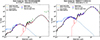 |
Fig. 4. Examples of our best-fit SEDs. The left panel shows the best-fit SED for an LSB with only upper limits in the MIR and FIR wavelengths, whereas the SED in the right panel is of an HSB with extensive photometry at all wavelengths. The black solid line is the model SED. The blue open diamonds and the red circles are the observed fluxes and best-fit model fluxes, respectively. The green downward triangles are the observed flux upper limits used in the SED fitting. |
3.2. Robustness of the SED fitting results
The robustness of the estimated physical parameters from our SED fit was verified by several tests. For each parameter in this work, we used the Bayesian mean and standard deviation of the quantities estimated by CIGALE based on the probability distribution function of the tested models, rather than directly using the best-fit model parameter. This ensured a more robust estimate of a quantity and its uncertainty, especially in case of degeneracy between physical parameters.
Another feature we used to check the reliability of the estimated parameters was a mock analysis provided by CIGALE. In this test, CIGALE builds a mock catalog with synthetic fluxes for each object based on its best-fit SED. The synthetic fluxes of each filter are modified by adding a random noise based on the uncertainty of the observed fluxes in the corresponding filter. Later, CIGALE performs the same calculations on this mock catalog as done for the original observations to get the mock physical parameters. The results of the mock analysis are given in Appendix A.1. We observed that the stellar mass is the most well-constrained quantity, with the square of the Pearson correlation coefficient (r2) equal to 0.99, followed by the total infrared luminosity (r2 = 0.85), the SFR (r2 = 0.81), and the V-band attenuation (r2 = 0.77). Although the SFR, LIR, and AV have a larger scatter (0.41 dex, 0.31 dex, and 0.14 mag, respectively), based on the linear regression analysis shown in Fig. A.1, we can still consider them reliable as estimates.
We also performed yet another test to verify the robustness of our estimated physical quantities. A separate SED fitting, similar to our original fits, was done for only the FIR-detected galaxies in our sample (53 galaxies with detection in either Herschel PACS or SPIRE), but this time only using their optical ugrizy-band photometry. This was done to check how well we could recover the “true” quantities by only using the ugrizy photometry. We compared the results of this fit with our original fit results and found that for the FIR-detected galaxies, the Mstar, SFR, LIR, and AV obtained from the original fit and the optical-only fit have a mean difference of −0.09 dex, −0.26 dex, −0.24 dex, and −0.07 mag, respectively, as given in Fig. A.2. The negative values indicate that a fit using only optical bands (or galaxies with only optical detection) in general has overestimated quantities, but only by a few tenths of an order of magnitude. We verified that this trend remains the same for our entire sample if we perform the SED fitting without using any flux upper limits in the MIR and FIR range. Similarly, we examined how a change in our upper limit definitions, from 5σ to 2σ, in the SED fitting affects our results. Such a change only has a negligible effect on our overall results, with the stellar mass remaining unchanged and the SFR, LIR, and AV changing by only 0.05 dex, 0.16 dex, and 0.02 mag. Table B.1 provides all the estimated parameters of our sample.
4. Results
Figure 5 shows the distribution of several physical parameters (stellar mass, stellar mass surface density, SFR, LIR, and AV) obtained after the SED fitting discussed in Sect. 3. Our sample predominantly consists of low-mass galaxies, with both the LSBs and HSBs having a median stellar mass of 108.3 M⊙ and 108.8 M⊙, respectively. The HRS sample lies along the massive end of the distribution, with a median stellar mass of 109.5 M⊙. Using the stellar mass and the measured radius (as discussed in Sect. 2.1.2), we estimated the stellar mass surface densities (Σstar) of our sample following Cortese et al. (2012b), as shown in Eq. (1):
 (1)
(1)
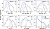 |
Fig. 5. Distribution of the best-fit parameters of our NEP sample obtained from the SED fitting. The LSBs and HSBs are marked as the blue solid and the green dashed histograms, respectively. The HRS comparison sample used in this work is shown as the brown dash-dotted distribution. The median values corresponding to each parameter are marked inside the panels in blue, green, and brown colors for the LSBs, HSBs, and the HRS sample, respectively. The bottom-right panel gives the reduced χ2 obtained from the SED fitting, and the black vertical dashed line in the panel marks the arbitrary selection cut we used to remove bad fits. |
where Re is the r-band half-light radius and Mstar is the stellar mass. Equation (1) is a widely used method in the literature to estimate Σstar for both LSBs and HSBs (e.g., Kauffmann et al. 2003; Zhong et al. 2010; Cortese et al. 2012b; Grootes et al. 2013; Boselli et al. 2022; Carleton et al. 2023). Although several other methods also exist to obtain Σstar, many of them provide similar values without changing the global properties of our sample. For instance, we tried estimating Σstar following Chamba et al. (2022)8 by using our observed  and the stellar mass-to-light ratio (M/L) obtained from the SED fitting (ratio of the stellar mass and the observed r-band luminosity). Notably, this method does not rely on the measured Re values as in Eq. (1). We found that the Σstar estimates from both methods are similar and have a mean difference of −0.15 dex (in general, the second method gives a slightly higher Σstar). However, we note that the two methods only provide an average value of the Σstar of a galaxy, and therefore such minor differences connected to the adopted methodology can be neglected. Estimating the “true” value of Σstar requires resolving individual stellar populations as well as information on the radial distribution of dust that can affect Σstar measurements. With our current data, such a task was beyond the scope of our work. Therefore, we adopted the Σstar values estimated using the simple and widely used method from Eq. (1). The distribution of the values is shown in Fig. 5.
The Σstar also follow a distribution similar to the stellar mass: the LSBs and HSBs have a median Σstar of 106.9 M⊙ kpc−2 and 107.4 M⊙ kpc−2, respectively, whereas the HRS sample has a value of 107.8 M⊙ kpc−2. In terms of the SFR, the LSBs and HSBs have a median SFR of 10−2.2 M⊙ yr−1 and 10−1.6 M⊙ yr−1, respectively, and the HRS galaxies have a corresponding value of 10−0.4 M⊙ yr−1. The LIR shows a distribution similar to the SFR, with the LSB, HSB, and the HRS galaxies having median values of 107.4 L⊙, 107.7 L⊙, and 109.3 L⊙, respectively. Figure 5 also shows the distribution of the V-band dust attenuation. For both the LSBs and HSBs, we found a median AV of 0.1 mag, with AV values ranging from almost zero to 2 mag. The HRS sample has a higher median AV of 0.4 mag. From the above comparison of the physical parameters, we saw that our sample extends toward the low-mass regime and has much lower SFR, LIR, and AV values than the HRS sample.
In the following subsections, we investigate the dependence of these quantities as a continuous function of Σstar in an attempt to understand how the geometrical distribution of stars within galaxies affects their global parameters. We chose the Σstar over  for our comparisons due to several reasons: The Σstar is a widely used quantity in the literature to compare the physical properties of galaxies and provides a more intrinsic physical quantity than
  . Moreover, although
  is a directly observed quantity, its value depends highly on the choice of an observed filter, whereas Σstar is less affected by such a choice. In the Sect. 4.1 we show a comparison of the
  and Σstar of our sample.
4.1. Optical surface brightness
The surface brightness of a galaxy is the distribution of its stellar light per unit area. It is related to the total stellar mass surface density of a galaxy in the same way as galaxy luminosity and stellar mass are related by their mass-to-light ratio. Although there are several relations in the literature that explore the connections between galaxy surface brightness, luminosity, and stellar mass (e.g., Boselli et al. 2008; Martin et al. 2019; Jackson et al. 2021), there exists a large scatter among such relations. For instance, Jackson et al. (2021) illustrates that for a fixed stellar mass, galaxies show a large scatter in their surface brightness up to ∼3 mag arcsec−2, ranging from LSBs to HSBs. Although it is well known that the stellar mass is one of the main drivers of galaxies’ properties (e.g., Kauffmann et al. 2003; Speagle et al. 2014), considering that a large scatter exists at any given stellar mass for the surface brightness, it is important to explore the possible trends in surface brightness associated with other quantities. In Fig. 6, we explore such a relation using our observed  and the stellar mass surface density (Σstar).
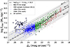 |
Fig. 6. Stellar mass surface density (Σstar) as a function of the r-band average surface brightness within the effective radius ( |


Our sample covers a large range of surface brightness (approximately seven orders of magnitude) and stellar mass surface densities (3 dex) from bright to very faint galaxies. This is about four orders of magnitude deeper in surface brightness than the HRS sample. For the HSBs ( mag arcsec−2), the Σstar follows a linear trend with
  , consistent with the observations from the HRS sample. However, for the LSBs (
 mag arcsec−2, which the HRS sample does not probe), the brighter tail (
 mag arcsec−2) closely follows the linear trend of the HSBs, but the fainter end (
 mag arcsec−2) diverges from this trend to form a flattening of Σstar around 107 M⊙ kpc−2 for the faintest sources.
We made an error-weighted linear fit to the full sample (as shown in Fig. 6) to obtain a best-fit relation as given in Eq. (2),
 (2)
(2)
where  and Σstar are in mag arcsec−2 and M⊙ kpc2 units, respectively. Obviously, this relation is determined by the stellar mass-to-light ratio and its eventual dependence on the stellar mass surface density. Notably, we obtained a slope of −0.4, as it is expected only if the mass-to-light ratio does not depend on the stellar mass surface density. Our best-fit line lies very close to a constant mass-to-light ratio of 1 M⊙/L⊙ (see Fig. 6). The majority of our sample is within the 3σ confidence level of the best-fit line (gray shaded region in Fig. 6), and only about 2.5% of the sample (38 galaxies, among which 36 are LSBs and 2 are HSBs) lies outside the 3σ range of the best-fit. These outliers are mostly LSBs with a high stellar mass surface density. This indicates a higher mass-to-light ratio for these galaxies. Using the r-band luminosities and the stellar masses of our sample, we estimated that the outliers have a median M/Lr of 3.4 M⊙/L⊙, compared to 1.1 M⊙/L⊙ for the full sample, making them distinct outliers.
Since the definition of our outliers given in Fig. 6 depends on the choice of the degree of the fit, we also performed a test with a polynomial fit of order two. We found that the polynomial fit provides a better fit with smaller residuals than the linear fit and reduces the number of outliers from 38 to 11. However, such a fit can also be affected by any incompleteness at the low surface brightness range. Moreover, in the polynomial fit, we lost an important piece of information that we have in the linear fit. The linear fit reproduces the trend in the HSB regime very well, and the outliers in the LSB regime are clearly a population of galaxies that are distinct from their HSB counterparts, as they lie in a range of high fiducial M/L ratio. This is a very distinct behavior, and we are interested in studying such cases. Therefore, we adopted the linear fit as given in Eq. (2) and the 38 outliers obtained from it.
4.2. Specific star formation rate
Figure 7 shows the dependence of the specific star formation rate (sSFR) of our sample as a function of the stellar mass surface density. The majority of our sample (∼73%) are star-forming galaxies with sSFR > 10−11 yr−1 (Boselli et al. 2023). We observed that for the star-forming galaxies, the sSFR is mostly flat with respect to the stellar mass surface density, but with a slight indication of a decrease in sSFR from the low to the high stellar mass surface density until Σstar ∼ 108 M⊙ kpc−2. Beyond this value, the sSFR shows a sudden decline to reach the population of quiescent galaxies (with a large scatter and big uncertainty in the sSFR of the order of ∼1 dex for quiescent galaxies). This trend is similar to what is observed in the HRS sample too, although the HRS sample, on average, has a higher sSFR than our sample. Interestingly, the outliers discussed in Sect. 4.1 lie equally along the star-forming and quiescent part of the sample. The LSBs and HSBs, on average, have very similar sSFR values (median log sSFR of −10.5 yr−1 for the LSBs and −10.4 yr−1 for the HSBs), in comparison to the slightly higher sSFR of the HRS galaxies (median log sSFR of −9.9 yr−1). Our sample, therefore, brings an important extension of the sSFR–Σstar relation in the regime of LSBs.
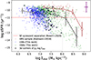 |
Fig. 7. Relationship between the specific star formation rate and stellar mass surface density. The symbols are the same as in Fig. 6. The red dashed line marks the separation of star-forming and quiescent galaxies (Boselli et al. 2023). The mean uncertainty of the sample obtained by propagating errors on individual measurements is given as the magenta error bar in the top-right corner. |
4.3. Specific infrared luminosity
Estimating the dust mass of galaxies requires a proper constraint on the peak of the FIR emission. However, considering the data we have for our sample, it is not possible to determine the dust masses. Therefore, we used the total IR luminosity of our sample obtained from the SED fitting9 discussed in Sect. 3 as a proxy for the dust mass (e.g., da Cunha et al. 2010; Orellana et al. 2017). Similarly, the ratio of the LIR and stellar mass (LIR/Mstar, which we refer to here as the “specific infrared luminosity”, or the sLIR) was used to probe the specific dust mass (Mdust/Mstar) of our sample. The specific dust mass of galaxies is an important measure of dust production (e.g., Cortese et al. 2012b; Casasola et al. 2020) as well as dust destruction processes and dust reformation mechanisms (e.g., Casasola et al. 2020; Donevski et al. 2020).
Figure 8 shows the variation in the specific infrared luminosity as a function of the stellar mass surface density. At the brightest end of Fig. 8, the sLIR rises steeply with decreasing stellar mass surface density until Σstar ∼ 108 M⊙ kpc−2, which is similar to the trend seen in Fig. 7 for the sSFR of quiescent galaxies. This steep rise was observed for the HRS sample too. Below Σstar ∼ 108 M⊙ kpc−2, the sLIR remains mostly flat toward lower stellar mass surface densities, as also seen in the HRS sample, which nonetheless lies along the higher sLIR part of the sample. Therefore, our sample allowed us to explore the trend of increasing specific dust content with decreasing stellar density at lower densities than what was found in the HRS. We found that dust emission is present at low densities, but there is saturation in the specific dust content rather than an increase. Moreover, similar to what was observed with the sSFR, both the LSBs and HSBs in our sample, on average, have comparable sLIR values of 10−0.9 L⊙/M⊙ and 10−1.1 L⊙/M⊙, respectively. The HRS, on the other hand, lies along the higher sLIR tail of the distribution with a median value of 10−0.2 L⊙/M⊙. A fraction of our HSBs also has sLIR similar to what is found in HRS. The outliers from the  –Σstar relation occupies the transition region of low to high sLIR, with many having high sLIR values as the HRS sample. Therefore, from the distribution given in Fig. 8, we can infer that LSBs have similar sLIR values to that of HSBs, although they have a lower absolute LIR. Moreover, since we observed a similar trend in both the sLIR and sSFR, these two quantities might be related. However, it is hard to disentangle them based on star formation activity and dust emission since we do not know much about the infrared properties of such galaxies.
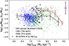 |
Fig. 8. Specific infrared luminosity (LIR per unit stellar mass) as a function of the stellar mass surface density. The symbols are the same as the previous figures. The mean uncertainty of the sample obtained by propagating errors on individual measurements is given as the magenta errorbar in the top-right corner. |
4.4. Dust attenuation
Figure 9 shows the V-band dust attenuation of the sample with respect to the stellar mass surface density. The majority of our sample (∼60%) have a low attenuation (i.e., AV < 0.1 mag). For the highest Σstar sources, which are well constrained with small uncertainties, we observed a higher attenuation but with a large scatter. For the fainter galaxies, the attenuation steeply decreases to reach an almost negligible value close to zero. However, the uncertainties associated with the AV estimates of many of these faint sources are typically large. For instance, the galaxies with Σstar < 107 M⊙ kpc−2 and with AV > 0.5 have an uncertainty in AV estimation of the order of 0.4 mag, making it hard to draw conclusions on them. Nevertheless, we still observed several faint galaxies with significant attenuation and small uncertainties. The 3σ outliers of the  –Σstar relation discussed in Sect. 4.1 (38 galaxies) are among those that appear to be in an interesting group in terms of attenuation. From Fig. 9, we observed that about 60% of the outliers (23 out of 38 galaxies) have a large attenuation, with AV > 0.5 mag and a mean value of 0.8 ± 0.2 mag. Moreover, several of these outliers were also detected in the IRAC bands, similar to the IRAC-detected LSBs from Hinz et al. (2007). However, none of the outliers have any detection in the MIR or FIR range.
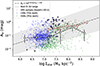 |
Fig. 9. V-band attenuation of the sample as a function of the stellar mass surface density. The black dot-dashed line is the best-fit line for our sample, and the gray shaded region is its corresponding 3σ uncertainty. The black open circles around some sources are the 3σ outliers of the |

Following Boselli et al. (2023), who derived a relation between attenuation and stellar mass, we did an error-weighted fit to our data to find a similar relation between AV and Σstar of our sample as given in Eq. (3):
 (3)
(3)
Our best-fit relation also follows a trend where the AV is less than 0.1 mag for the faint galaxies until Σstar ∼ 107 M⊙ kpc−2, beyond which we observed a steep rise in the AV for the brighter galaxies, albeit with a large scatter (we note that the scatter shown in Fig. 9 is in logarithmic scale). The HRS sample shows a similar trend in attenuation with the stellar mass surface density, although it generally has a larger AV than our sample for the same Σstar, but it is consistent with the large scatter seen in this range. We note that only the late-type galaxies from the HRS sample have measurements in AV available (see Sect. 2.2). This explains the lack of high Σstar HRS galaxies with attenuation close to zero observed in our sample.
We also found that the steep rise of AV in Fig. 9 is largely driven by the galaxies at Σstar > 108 M⊙ kpc−2 that are dominated by more massive HSBs (we do not have any LSBs beyond this Σstar value). So the trend in the AV we observed here is also linked to its dependence on the stellar mass, which is well known (e.g., Bogdanoska & Burgarella 2020; Riccio et al. 2021; Boselli et al. 2023). However, in the range of Σstar < 108 M⊙ kpc−2, we have a large overlap with the LSBs and HSBs of stellar masses mostly in the range of 108 − 109 M⊙. They are both consistent with low attenuation, except for the LSB outliers that remain a peculiar population with high attenuation.
5. Discussion
5.1. Dust content of low surface brightness galaxies
The results given in Sect. 4.4 show that the majority of the LSBs in our sample ( mag arcsec−2, or approximately Σstar < 107 M⊙ kpc−2)10 have a very low amount of dust attenuation. Among the LSBs (1003 out of 1631 galaxies), about 80% have a negligible attenuation, with an AV < 0.2 mag and a median attenuation of ∼0.09 mag. This is consistent with only a few other observations of LSBs from the literature where extreme LSBs, like the ultra-diffuse galaxies (UDGs), were found to have a very low attenuation, with a median AV of ∼0.1 mag (Pandya et al. 2018; Barbosa et al. 2020; Buzzo et al. 2022). However, Liang et al. (2010) found a median AV of 0.46 mag for their sample of LSBs from the SDSS survey. The higher attenuation in their LSB sample could be attributed to the fact that the LSBs from Liang et al. (2010) are massive galaxies with a median stellar mass of 109.5 M⊙, which contrasts with our low-mass LSBs with a median stellar mass of 108.3 M⊙. Moreover, the AV values from Liang et al. (2010) were computed from the Balmer decrement without applying a correction for the differential attenuation of nebular lines and the continuum as shown in Table 1. Applying such a correction would reduce their median AV to ∼0.2 mag, which is close to the values we observed for our sample of LSBs. Only about 4% of the LSBs in our sample (2.5% of the total sample) have a significant attenuation, that is, an AV > 0.5 mag. These are the 3σ outliers from the
  –Σstar relation as shown Figs. 6 and 9. This could indicate that a fraction of the LSBs with high stellar mass-to-light ratios (M/Lr > 3 M⊙/L⊙) have a higher attenuation.
We also looked into how much the attenuation affects the position of the outliers in the  –Σstar relation. For this purpose, we applied a correction for the observed surface brightness of the outliers using the estimated AV values. We converted the V-band attenuation to the attenuation in the HSC r-band using the Calzetti et al. (2000) attenuation law before correcting for the r-band surface brightness. Figure 10 shows the change in the position of the outliers after the attenuation correction. All the outlier LSBs remained LSBs with
  mag arcsec−2. However, we observed that about 50% of them moved into the 3σ confidence range of the
  –Σstar relation after the attenuation was corrected. This indicates that the effect of attenuation plays a significant role in making a fraction of the LSBs appear fainter in the observations. However, attenuation alone cannot explain all the outliers in our
  –Σstar relation.
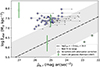 |
Fig. 10. 3σ outliers of the surface brightness-stellar mass surface density linear relation discussed in Sect. 4.1. The black arrows indicate the directions/positional changes on this plane, and how the outliers (open circles) will move after the correction for the r-band attenuation. The green diamond symbols mark the location of three giant LSB galaxies (Malin 1, UGC 9024, and UGC 6614, from the left to right, respectively) from the literature (Rahman et al. 2007). The black dash-dotted and the gray shaded region is the best-fit line and its 3σ confidence range as described in Sect. 4.1. |
Giant low surface brightness galaxies (GLSBs) are another interesting and extreme class of objects among LSBs (e.g., Sprayberry et al. 1995; Hagen et al. 2016; Junais et al. 2020). The infrared properties of three GLSBs (Malin 1, UGC 6614, and UGC 9024) were explored by Rahman et al. (2007) using Spitzer observations. All of them were undetected at MIR and FIR wavelengths, allowing only the upper limits in their infrared properties to be obtained. Figure 10 shows a comparison of their stellar mass surface density11 and surface brightness12 as compared to our sample. We saw that two out of the three GLSBs (Malin 1 and UGC 6614) are 3σ outliers from the  –Σstar relation. Moreover, their sSFR and sLIR are also consistent with our sample (based on Rahman et al. 2007, the three GLSBs have an sSFR of 10−10.8, 10−10.2, and 10−10.4 yr−1 as well as an sLIR of 10−0.9, 10−0.4, and 10−0.5 L⊙/M⊙, respectively). Therefore, as shown in Fig. 10, it is likely that these GLSBs also have a significant dust attenuation, similar to the outliers we observed in our sample, although their previous infrared observations do not provide any estimate of attenuation.
Apart from the observational data on GLSBs, Kulier et al. (2020) provided some estimates on the dust attenuation of GLSBs from the EAGLE simulations (see their Fig. A.2). They obtained an average AV of 0.15 mag for their simulated GLSB sample, with a range of values extending from AV = 0.4 mag for the brighter sources ( mag arcsec−2) to AV = 0.05 mag for the faintest ones (
 mag arcsec−2). Therefore, comparing our results with observations and simulations allowed us to anticipate the presence of some detectable dust attenuation in GLSBs as well.
5.2. Possible caveats
The analyses presented in this work may be affected by several aspects. Firstly, since we attempted to study the optical as well as infrared properties of our sample (surface brightness, radius, stellar mass, SFR, total infrared luminosity, and dust attenuation), we required extensive multiwavelength data coverage in the UV to FIR range. However, as noted in Sect. 2.1.3, for approximately 85% of our sample, the deep 5σ upper limits can only be provided in the MIR to FIR regime (from the 7 μm to 500 μm wavelength range). In those cases, the detection limits were used to put constraints on the infrared emission of the SED. Such an approach can introduce significant uncertainties in the estimated infrared properties of our sample (especially in the LIR and AV). We performed several tests to quantify and minimize the effect of such uncertainties on our results (see Sect. 3.2 for more details on the robustness of the estimated parameters). Additionally, our sample selection, with the requirement to have a u-band detection, was aimed at minimizing such uncertainties. The u-band, being close to the UV part of the spectrum, is more sensitive to the effects of dust attenuation and thereby the re-emission in the infrared.
Another potential uncertainty in our results arises from a possible redshift dependence of the quantities. However, considering the very narrow range of redshift used in this work (z < 0.1) and the fact that we used redshift-independent quantities, we do not expect such a dependence to have an impact. We verified that there are no significant variations in our sample with the redshift, and our results remained unchanged. The accuracy of the photometric redshift estimates from Huang et al. (2021) used in this work can be yet another source of uncertainty. Considering the very faint nature of the majority of our sample, it was not feasible to obtain spectroscopic redshifts for all of them (all the galaxies with spectroscopic redshifts in our sample are HSBs, as shown in Table B.1). Also, as discussed in Sect. 2.1.1, in general, the photometric redshift estimates we used have a higher accuracy and a lower catastrophic outlier rate. The presence of the u-band also significantly improves the photometric redshift estimates, as noted by Huang et al. (2021). Nevertheless, we made an estimate of the effect of the photometric redshift uncertainty on our measured physical quantities. For a typical redshift uncertainty of σzp = 0.06 for our sample (as discussed in Sect. 2.1.1), we found that, on average, the Mstar and Re changes by a large factor (0.47 dex and 0.21 dex, respectively). However, since we computed the Σstar as a ratio of Mstar and Re, as given in Eq. (1), they cancel each other, and thus the Σstar values have only a 0.04 dex difference regarding the change in redshift, making Σstar an almost redshift-independent quantity. In the case of the sSFR, sLIR, and AV, we also only saw a negligible difference (0.13 dex, 0.04 dex, and 0 dex, respectively).
Therefore, considering all the above potential caveats, we conclude that our estimates are still robust within the uncertainties discussed. The approach we used in this work will be useful for constraining the physical quantities of LSBs with only limited multiwavelength counterparts, especially with upcoming surveys, such as LSST, that will observe thousands of LSBs in the ugrizy-bands.
6. Conclusions
We present an optically selected sample of 1631 galaxies at z < 0.1 from the NEP Wide field. We crossmatched this sample with several multiwavelength sets of available data ranging from UV to FIR and performed an SED fitting procedure to obtain key physical parameters, such as stellar mass, SFR, LIR, and AV. We also extracted radial surface brightness profiles for the sample and estimated their average optical surface brightness and sizes. Our main results can be summarized as follows:
-
Using the measured average r-band surface brightness (
 ), our sample consists of 1003 LSBs (
 > 23 mag arcsec−2) and 628 HSBs (
 ≤ 23 mag arcsec−2).
 -
The LSBs have a median stellar mass, surface brightness, and effective radius of 108.3 M⊙, 23.8 mag arcsec−2, and 1.9 kpc, respectively. For the HSBs, the corresponding median values are 108.8 M⊙, 22.2 mag arcsec−2, and 2.2 kpc. Similarly, the LSBs have a median SFR and LIR of 10−2.2 M⊙ yr−1 and 107.4 L⊙, in comparison to 10−1.6 M⊙ yr−1 and 107.7 L⊙ for the HSBs. For both the LSBs and HSBs, we found a median AV of 0.1 mag.
-
A comparison of the surface brightness (
 ) as a function of the stellar mass surface density (Σstar) showed that our sample follows the linear trend for the HSBs, which is consistent with the HRS sample from the literature. However, for the LSBs, we observed several outliers from the linear
  –Σstar relation, indicating a higher mass-to-light ratio for them. Most of these outliers also have a high dust attenuation.
 -
We analyzed the variation in the sSFR and sLIR of our sample with respect to their stellar mass surface density. Among the star-forming galaxies (sSFR > 10−11 yr−1), the sSFR is mostly flat with respect to the change in stellar mass surface density but with a slight indication of an increase in sSFR for the lowest Σstar galaxies. The sSFR steeply declines for the highest Σstar sources that are quiescent. A similar trend was observed for the sLIR, too. We find that both the LSBs and HSBs in our sample have a comparable average sSFR and sLIR. The HRS sample, in general, lies along the higher sSFR and sLIR regime compared to our sample, but they are consistent and agree within the scatter we observed.
-
The change in dust attenuation with the stellar mass surface density of our sample shows that galaxies with a higher Σstar have a larger AV and scatter, contrary to the flat, decreasing trend observed for the specific dust luminosity. The dust attenuation steeply declines and becomes close to zero for the majority of LSBs. However, in about 4% of the LSBs that are outliers, we observed a significant attenuation with a mean AV of 0.8 mag, showing that not all the LSBs are dust poor. Moreover, the extreme giant LSBs in the literature also show some similarities to these outlier LSBs, indicating the presence of more dust content in them than previously thought.
This work provides measurements that can be further tested using current as well as upcoming observations from LSST and JWST, where a large number LSBs and HSBs will be observed at unprecedented depth. The LSST will provide deep optical imaging data over large areas of the sky, allowing for a detailed study of the statistical properties of galaxies, including LSBs. In addition, JWST’s high sensitivity and resolution imaging in the near-infrared and MIR regimes, as well its spectroscopic capabilities, will enable a comprehensive study of the infrared properties of such galaxies, including their dust content, gas metallicity, and star formation activity. The data from these facilities will complement this work to provide a clear picture of the properties of LSBs in the context of galaxy evolution.
The CFHT Megcam/Megaprime observations of the NEP field covers only a total area of ∼3.6 deg2, compared to the ∼5.4 deg2 covered by the HSC observations.
We note that at this depth, many local bright galaxies are saturated in the HSC observations, and they were removed as flagged sources with bad pixels by Huang et al. (2021).
The photometric redshift accuracy σzp from Huang et al. (2021) is defined as the normalized median absolute deviation, where  , with zp and zs being the photometric and spectroscopic redshifts, respectively.
We used the AKARI and Herschel/SPIRE upper limits given in Table 1 of Kim et al. (2021), as they have the deepest coverage in the entire NEP Wide field for the MIR and FIR range.
Adopting different metallicity values was found to have only a negligible impact on the overall results presented in this paper. Therefore, as we focus mainly on LSBs, we chose to keep the metallicity at a subsolar value in order to reduce the number of free parameters in our fitting procedure.
We verified that a variation in the interstellar radiation field slope α from two to three does not make any significant change (a change of less than 0.1 dex on all our estimated quantities) in our SED results.
Following Chamba et al. (2022), the Σstar of our sample can also be estimated as log Σstar (M⊙ pc−2) = 0.4 × (Mr,⊙ − μr) + log M/Lr + 8.629, where Mr, ⊙ is the absolute magnitude of the sun in the r-band filter (Mr, ⊙ = 4.64 mag for HSC r-band) and μr and M/Lr are the r-band surface brightness and stellar mass-to-light ratio, respectively.
The LIR values from CIGALE were computed by integrating the full dust emission model (shown as the red solid curves in Fig. 4) over an arbitrarily large wavelength range used in the modeling. This should, in practice, give very similar values as the LIR commonly estimated in the literature within the wavelength range of 8−1000 μm.
A stellar mass surface density of 107 M⊙ kpc−2 corresponds to an average r-band surface brightness ( ) of 23.2 mag arcsec−2, based on the Eq. (2).
The stellar masses and sizes of the GLSBs were taken from Rahman et al. (2007) and Comparat et al. (2017), respectively, to estimate their stellar mass surface densities.
The  values of the GLSBs were estimated by using the B-band central surface brightness (μ0, B) values from Rahman et al. (2007). The μ0, B values were converted to the r-band
  assuming a constant Sérsic index n = 1 (Graham & Driver 2005) and a constant B − r color of 0.6 mag.
Acknowledgments
J. and K.M. are grateful for support from the Polish National Science Centre via grant UMO-2018/30/E/ST9/00082. W.J.P. has been supported by the Polish National Science Center project UMO-2020/37/B/ST9/00466 and by the Foundation for Polish Science (FNP). J.K. acknowledges support from NSF through grants AST-1812847 and AST-2006600. M.R. acknowledges support from the Narodowe Centrum Nauki (UMO-2020/38/E/ST9/00077). M.B. gratefully acknowledges support by the ANID BASAL project FB210003 and from the FONDECYT regular grant 1211000. D.D. acknowledges support from the National Science Center (NCN) grant SONATA (UMO-2020/39/D/ST9/00720). D.D. also acknowledges support from the SISSA visiting research programme. A.P. acknowledges the Polish National Science Centre grant UMO-2018/30/M/ST9/00757 and the Polish Ministry of Science and Higher Education grant DIR/WK/2018/12.
References
- Andreani, P., Boselli, A., Ciesla, L., et al. 2018, A&A, 617, A33 [NASA ADS] [CrossRef] [EDP Sciences] [Google Scholar]
- Arnouts, S., Cristiani, S., Moscardini, L., et al. 1999, MNRAS, 310, 540 [Google Scholar]
- Barbosa, C. E., Zaritsky, D., Donnerstein, R., et al. 2020, ApJS, 247, 46 [Google Scholar]
- Bell, E. F., Barnaby, D., Bower, R. G., et al. 2000, MNRAS, 312, 470 [NASA ADS] [CrossRef] [Google Scholar]
- Bianchi, L., Shiao, B., & Thilker, D. 2017, ApJS, 230, 24 [Google Scholar]
- Bianco, F. B., Ivezić, Ž., Jones, R. L., et al. 2022, ApJS, 258, 1 [NASA ADS] [CrossRef] [Google Scholar]
- Bigiel, F., Leroy, A., Walter, F., et al. 2010, AJ, 140, 1194 [NASA ADS] [CrossRef] [Google Scholar]
- Blanton, M. R., Lupton, R. H., Schlegel, D. J., et al. 2005, ApJ, 631, 208 [Google Scholar]
- Bogdanoska, J., & Burgarella, D. 2020, MNRAS, 496, 5341 [NASA ADS] [CrossRef] [Google Scholar]
- Boissier, S., Gil de Paz, A., Boselli, A., et al. 2008, ApJ, 681, 244 [NASA ADS] [CrossRef] [Google Scholar]
- Boquien, M., Burgarella, D., Roehlly, Y., et al. 2019, A&A, 622, A103 [NASA ADS] [CrossRef] [EDP Sciences] [Google Scholar]
- Boselli, A., Boissier, S., Cortese, L., & Gavazzi, G. 2008, A&A, 489, 1015 [CrossRef] [EDP Sciences] [Google Scholar]
- Boselli, A., Eales, S., Cortese, L., et al. 2010, PASP, 122, 261 [Google Scholar]
- Boselli, A., Fossati, M., Gavazzi, G., et al. 2015, A&A, 579, A102 [NASA ADS] [CrossRef] [EDP Sciences] [Google Scholar]
- Boselli, A., Fossati, M., & Sun, M. 2022, A&ARv, 30, 3 [NASA ADS] [CrossRef] [Google Scholar]
- Boselli, A., Fossati, M., Roediger, J., et al. 2023, A&A, 669, A73 [NASA ADS] [CrossRef] [EDP Sciences] [Google Scholar]
- Bothun, G., Impey, C., & McGaugh, S. 1997, PASP, 109, 745 [NASA ADS] [CrossRef] [Google Scholar]
- Bruzual, G., & Charlot, S. 2003, MNRAS, 344, 1000 [NASA ADS] [CrossRef] [Google Scholar]
- Buzzo, M. L., Forbes, D. A., Brodie, J. P., et al. 2022, MNRAS, 517, 2231 [NASA ADS] [CrossRef] [Google Scholar]
- Calzetti, D., Armus, L., Bohlin, R. C., et al. 2000, ApJ, 533, 682 [NASA ADS] [CrossRef] [Google Scholar]
- Cardelli, J. A., Clayton, G. C., & Mathis, J. S. 1989, ApJ, 345, 245 [Google Scholar]
- Carleton, T., Cohen, S. H., Frye, B., et al. 2023, ApJ, submitted [arXiv:2303.04726] [Google Scholar]
- Casasola, V., Bianchi, S., De Vis, P., et al. 2020, A&A, 633, A100 [NASA ADS] [CrossRef] [EDP Sciences] [Google Scholar]
- Chabrier, G. 2003, PASP, 115, 763 [Google Scholar]
- Chamba, N., Trujillo, I., & Knapen, J. H. 2022, A&A, 667, A87 [NASA ADS] [CrossRef] [EDP Sciences] [Google Scholar]
- Ciesla, L., Boquien, M., Boselli, A., et al. 2014, A&A, 565, A128 [NASA ADS] [CrossRef] [EDP Sciences] [Google Scholar]
- Ciesla, L., Elbaz, D., & Fensch, J. 2017, A&A, 608, A41 [NASA ADS] [CrossRef] [EDP Sciences] [Google Scholar]
- Ciesla, L., Buat, V., Boquien, M., et al. 2021, A&A, 653, A6 [NASA ADS] [CrossRef] [EDP Sciences] [Google Scholar]
- Comparat, J., Maraston, C., Goddard, D., et al. 2017, ArXiv e-prints [arXiv:1711.06575] [Google Scholar]
- Cortese, L., Boissier, S., Boselli, A., et al. 2012a, A&A, 544, A101 [NASA ADS] [CrossRef] [EDP Sciences] [Google Scholar]
- Cortese, L., Ciesla, L., Boselli, A., et al. 2012b, A&A, 540, A52 [NASA ADS] [CrossRef] [EDP Sciences] [Google Scholar]
- da Cunha, E., Eminian, C., Charlot, S., & Blaizot, J. 2010, MNRAS, 403, 1894 [Google Scholar]
- Dale, D. A., Helou, G., Magdis, G. E., et al. 2014, ApJ, 784, 83 [Google Scholar]
- de Blok, W. J. G., McGaugh, S. S., & van der Hulst, J. M. 1996, MNRAS, 283, 18 [NASA ADS] [CrossRef] [Google Scholar]
- Donevski, D., Lapi, A., Małek, K., et al. 2020, A&A, 644, A144 [NASA ADS] [CrossRef] [EDP Sciences] [Google Scholar]
- Galaz, G., Herrera-Camus, R., Garcia-Lambas, D., & Padilla, N. 2011, ApJ, 728, 74 [NASA ADS] [CrossRef] [Google Scholar]
- Gardner, J. P., Mather, J. C., Clampin, M., et al. 2006, Space Sci. Rev., 123, 485 [Google Scholar]
- Gerritsen, J. P. E., & de Blok, W. J. G. 1999, A&A, 342, 655 [Google Scholar]
- Graham, A. W., & Driver, S. P. 2005, PASA, 22, 118 [NASA ADS] [CrossRef] [Google Scholar]
- Grootes, M. W., Tuffs, R. J., Popescu, C. C., et al. 2013, ApJ, 766, 59 [NASA ADS] [CrossRef] [Google Scholar]
- Hagen, L. M. Z., Seibert, M., Hagen, A., et al. 2016, ApJ, 826, 210 [NASA ADS] [CrossRef] [Google Scholar]
- Hinz, J. L., Rieke, M. J., Rieke, G. H., et al. 2007, ApJ, 663, 895 [NASA ADS] [CrossRef] [Google Scholar]
- Hinz, J. L., Rieke, M. J., Rieke, G. H., et al. 2008, ASP Conf. Ser., 381, 153 [Google Scholar]
- Holwerda, B. W., Gonzalez, R. A., Allen, R. J., & van der Kruit, P. C. 2005, AJ, 129, 1396 [NASA ADS] [CrossRef] [Google Scholar]
- Huang, T.-C., Matsuhara, H., Goto, T., et al. 2020, MNRAS, 498, 609 [NASA ADS] [CrossRef] [Google Scholar]
- Huang, T.-C., Matsuhara, H., Goto, T., et al. 2021, MNRAS, 506, 6063 [NASA ADS] [CrossRef] [Google Scholar]
- Hunt, L. K., De Looze, I., Boquien, M., et al. 2019, A&A, 621, A51 [NASA ADS] [CrossRef] [EDP Sciences] [Google Scholar]
- Ilbert, O., Arnouts, S., McCracken, H. J., et al. 2006, A&A, 457, 841 [NASA ADS] [CrossRef] [EDP Sciences] [Google Scholar]
- Ivezić, Ž., Kahn, S. M., Tyson, J. A., et al. 2019, ApJ, 873, 111 [Google Scholar]
- Jackson, R. A., Martin, G., Kaviraj, S., et al. 2021, MNRAS, 502, 4262 [NASA ADS] [CrossRef] [Google Scholar]
- Jarrett, T. H., Cohen, M., Masci, F., et al. 2011, ApJ, 735, 112 [Google Scholar]
- Jeon, Y., Im, M., Kang, E., Lee, H. M., & Matsuhara, H. 2014, ApJS, 214, 20 [NASA ADS] [CrossRef] [Google Scholar]
- Junais, S., Boissier, S., Epinat, B., et al. 2020, A&A, 637, A21 [NASA ADS] [CrossRef] [EDP Sciences] [Google Scholar]
- Junais, S., Boissier, S., Boselli, A., et al. 2022, A&A, 667, A76 [NASA ADS] [CrossRef] [EDP Sciences] [Google Scholar]
- Kauffmann, G., Heckman, T. M., White, S. D. M., et al. 2003, MNRAS, 341, 54 [Google Scholar]
- Kennicutt, R. C., & Evans, N. J. 2012, ARA&A, 50, 531 [NASA ADS] [CrossRef] [Google Scholar]
- Kim, S. J., Lee, H. M., Matsuhara, H., et al. 2012, A&A, 548, A29 [NASA ADS] [CrossRef] [EDP Sciences] [Google Scholar]
- Kim, S. J., Oi, N., Goto, T., et al. 2021, MNRAS, 500, 4078 [Google Scholar]
- Kim, J., Lee, J., Laigle, C., et al. 2023, ApJ, 951, 137 [NASA ADS] [CrossRef] [Google Scholar]
- Kniazev, A. Y., Grebel, E. K., Pustilnik, S. A., et al. 2004, AJ, 127, 704 [NASA ADS] [CrossRef] [Google Scholar]
- Kulier, A., Galaz, G., Padilla, N. D., & Trayford, J. W. 2020, MNRAS, 496, 3996 [NASA ADS] [CrossRef] [Google Scholar]
- Leitherer, C., Li, I. H., Calzetti, D., & Heckman, T. M. 2002, ApJS, 140, 303 [NASA ADS] [CrossRef] [Google Scholar]
- Liang, Y. C., Zhong, G. H., Hammer, F., et al. 2010, MNRAS, 409, 213 [NASA ADS] [CrossRef] [Google Scholar]
- Lupi, A., Sbarrato, T., & Carniani, S. 2020, MNRAS, 492, 2528 [NASA ADS] [CrossRef] [Google Scholar]
- Mahajan, S., Drinkwater, M. J., Driver, S., et al. 2018, MNRAS, 475, 788 [NASA ADS] [CrossRef] [Google Scholar]
- Martin, G., Kaviraj, S., Laigle, C., et al. 2019, MNRAS, 485, 796 [NASA ADS] [CrossRef] [Google Scholar]
- Matthews, L. D., van Driel, W., & Monnier-Ragaigne, D. 2001, A&A, 365, 1 [NASA ADS] [CrossRef] [EDP Sciences] [Google Scholar]
- Minchin, R. F., Disney, M. J., Parker, Q. A., et al. 2004, MNRAS, 355, 1303 [NASA ADS] [CrossRef] [Google Scholar]
- Nayyeri, H., Ghotbi, N., Cooray, A., et al. 2018, ApJS, 234, 38 [NASA ADS] [CrossRef] [Google Scholar]
- Noll, S., Burgarella, D., Giovannoli, E., et al. 2009, A&A, 507, 1793 [NASA ADS] [CrossRef] [EDP Sciences] [Google Scholar]
- Oi, N., Matsuhara, H., Murata, K., et al. 2014, A&A, 566, A60 [NASA ADS] [CrossRef] [EDP Sciences] [Google Scholar]
- Oi, N., Goto, T., Matsuhara, H., et al. 2021, MNRAS, 500, 5024 [Google Scholar]
- O’Neil, K., & Bothun, G. 2000, ApJ, 529, 811 [CrossRef] [Google Scholar]
- Orellana, G., Nagar, N. M., Elbaz, D., et al. 2017, A&A, 602, A68 [NASA ADS] [CrossRef] [EDP Sciences] [Google Scholar]
- Pandya, V., Romanowsky, A. J., Laine, S., et al. 2018, ApJ, 858, 29 [Google Scholar]
- Pearson, C., Cheale, R., Serjeant, S., et al. 2017, Publ. Korean Astron. Soc., 32, 219 [Google Scholar]
- Pearson, C., Barrufet, L., Campos Varillas, M. D. C., et al. 2019, PASJ, 71, 13 [NASA ADS] [CrossRef] [Google Scholar]
- Pearson, W. J., Suelves, L. E., Ho, S. C. C., et al. 2022, A&A, 661, A52 [NASA ADS] [CrossRef] [EDP Sciences] [Google Scholar]
- Peng, C. Y., Ho, L. C., Impey, C. D., & Rix, H.-W. 2002, AJ, 124, 266 [Google Scholar]
- Rahman, N., Howell, J. H., Helou, G., Mazzarella, J. M., & Buckalew, B. 2007, ApJ, 663, 908 [NASA ADS] [CrossRef] [Google Scholar]
- Reines, A. E., Greene, J. E., & Geha, M. 2013, ApJ, 775, 116 [Google Scholar]
- Riccio, G., Małek, K., Nanni, A., et al. 2021, A&A, 653, A107 [NASA ADS] [CrossRef] [EDP Sciences] [Google Scholar]
- Rodriguez-Gomez, V., Snyder, G. F., Lotz, J. M., et al. 2019, MNRAS, 483, 4140 [NASA ADS] [CrossRef] [Google Scholar]
- Sabatini, S., Davies, J., Scaramella, R., et al. 2003, MNRAS, 341, 981 [NASA ADS] [CrossRef] [Google Scholar]
- Sedgwick, T. M., Baldry, I. K., James, P. A., & Kelvin, L. S. 2019, MNRAS, 484, 5278 [Google Scholar]
- Speagle, J. S., Steinhardt, C. L., Capak, P. L., & Silverman, J. D. 2014, ApJS, 214, 15 [Google Scholar]
- Sprayberry, D., Impey, C. D., Bothun, G. D., & Irwin, M. J. 1995, AJ, 109, 558 [NASA ADS] [CrossRef] [Google Scholar]
- Stone, C. J., Arora, N., Courteau, S., & Cuillandre, J.-C. 2021, MNRAS, 508, 1870 [NASA ADS] [CrossRef] [Google Scholar]
- Williams, R. P., Baldry, I. K., Kelvin, L. S., et al. 2016, MNRAS, 463, 2746 [NASA ADS] [CrossRef] [Google Scholar]
- Wyder, T. K., Martin, D. C., Barlow, T. A., et al. 2009, ApJ, 696, 1834 [NASA ADS] [CrossRef] [Google Scholar]
- Zhong, G. H., Liang, Y. C., Hammer, F., et al. 2010, A&A, 520, A69 [NASA ADS] [CrossRef] [EDP Sciences] [Google Scholar]
Appendix A: Spectral energy distribution fitting robustness
A.1. Mock analysis
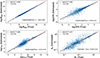 |
Fig. A.1. Mock analysis performed using CIGALE to compare the “true” values from the mock catalog with the Bayesian estimated values. The black dashed lines show the linear regression fit, and the corresponding regression coefficients (r2) are marked in each panel. The red dotted line is the one-to-one relation. The mean difference and scatter between the estimated and true values are marked in each panel. |
A.2. Comparison of fits with and without FIR data
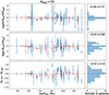 |
Fig. A.2. Comparison of the SED fitting results for the 53 FIR-detected galaxies using their full photometry from UV to FIR with respect to a fitting using only the optical ugrizy-bands. From top to bottom, the panels show the difference in SFR, LIR, and AV estimated from the two fits, as a function of the stellar mass of the galaxies. The red dashed line marks the mean and scatter along different stellar mass bins. The histograms beside each panel give the overall distribution of each quantity, with their mean and scatter indicated at the top of each histogram. When comparing the stellar mass estimates of the two fits, we found that there is only a minor difference, as expected, with a mean difference of −0.09 ± 0.13 dex. |
Appendix B: Data table with the physical properties of the sample
Estimated properties of the sample. The complete table is available at the CDS.
All Tables
Estimated properties of the sample. The complete table is available at the CDS.
All Figures
|
Fig. 1. Example of an r-band radial surface brightness profile extracted for a galaxy using AutoProf. The HSC r-band image of the galaxy is shown in the inset panel. The black dotted line marks the effective radius of the galaxy. The brown dashed horizontal line is the 1σ sky noise level. |
| In the text | |
|
Fig. 2. Distribution of the basic properties of the LSBs (blue solid line) and HSBs (green dashed line) in our sample. The average r-band surface brightness within the effective radius and the r-band absolute magnitude are given in the top-left and top-right panels, respectively. The redshift and the effective radius are in the bottom-left and bottom-right panels, respectively. The median values corresponding to each parameter are marked inside each panel in blue and green for the LSBs and HSBs, respectively. |
| In the text | |
|
Fig. 3. Distribution of the multiwavelength data available for the sample. The LSBs and HSBs are marked as the blue striped bars and the green dashed bars, respectively. The broadband filter names and their corresponding wavelengths are given in the bottom and top horizontal axes, respectively. All the galaxies in the sample have detection in the ugrizy-bands. |
| In the text | |
|
Fig. 4. Examples of our best-fit SEDs. The left panel shows the best-fit SED for an LSB with only upper limits in the MIR and FIR wavelengths, whereas the SED in the right panel is of an HSB with extensive photometry at all wavelengths. The black solid line is the model SED. The blue open diamonds and the red circles are the observed fluxes and best-fit model fluxes, respectively. The green downward triangles are the observed flux upper limits used in the SED fitting. |
| In the text | |
|
Fig. 5. Distribution of the best-fit parameters of our NEP sample obtained from the SED fitting. The LSBs and HSBs are marked as the blue solid and the green dashed histograms, respectively. The HRS comparison sample used in this work is shown as the brown dash-dotted distribution. The median values corresponding to each parameter are marked inside the panels in blue, green, and brown colors for the LSBs, HSBs, and the HRS sample, respectively. The bottom-right panel gives the reduced χ2 obtained from the SED fitting, and the black vertical dashed line in the panel marks the arbitrary selection cut we used to remove bad fits. |
| In the text | |
|
Fig. 6. Stellar mass surface density (Σstar) as a function of the r-band average surface brightness within the effective radius ( |
| In the text | |
|
Fig. 7. Relationship between the specific star formation rate and stellar mass surface density. The symbols are the same as in Fig. 6. The red dashed line marks the separation of star-forming and quiescent galaxies (Boselli et al. 2023). The mean uncertainty of the sample obtained by propagating errors on individual measurements is given as the magenta error bar in the top-right corner. |
| In the text | |
|
Fig. 8. Specific infrared luminosity (LIR per unit stellar mass) as a function of the stellar mass surface density. The symbols are the same as the previous figures. The mean uncertainty of the sample obtained by propagating errors on individual measurements is given as the magenta errorbar in the top-right corner. |
| In the text | |
|
Fig. 9. V-band attenuation of the sample as a function of the stellar mass surface density. The black dot-dashed line is the best-fit line for our sample, and the gray shaded region is its corresponding 3σ uncertainty. The black open circles around some sources are the 3σ outliers of the |
| In the text | |
|
Fig. 10. 3σ outliers of the surface brightness-stellar mass surface density linear relation discussed in Sect. 4.1. The black arrows indicate the directions/positional changes on this plane, and how the outliers (open circles) will move after the correction for the r-band attenuation. The green diamond symbols mark the location of three giant LSB galaxies (Malin 1, UGC 9024, and UGC 6614, from the left to right, respectively) from the literature (Rahman et al. 2007). The black dash-dotted and the gray shaded region is the best-fit line and its 3σ confidence range as described in Sect. 4.1. |
| In the text | |
|
Fig. A.1. Mock analysis performed using CIGALE to compare the “true” values from the mock catalog with the Bayesian estimated values. The black dashed lines show the linear regression fit, and the corresponding regression coefficients (r2) are marked in each panel. The red dotted line is the one-to-one relation. The mean difference and scatter between the estimated and true values are marked in each panel. |
| In the text | |
|
Fig. A.2. Comparison of the SED fitting results for the 53 FIR-detected galaxies using their full photometry from UV to FIR with respect to a fitting using only the optical ugrizy-bands. From top to bottom, the panels show the difference in SFR, LIR, and AV estimated from the two fits, as a function of the stellar mass of the galaxies. The red dashed line marks the mean and scatter along different stellar mass bins. The histograms beside each panel give the overall distribution of each quantity, with their mean and scatter indicated at the top of each histogram. When comparing the stellar mass estimates of the two fits, we found that there is only a minor difference, as expected, with a mean difference of −0.09 ± 0.13 dex. |
| In the text | |
Current usage metrics show cumulative count of Article Views (full-text article views including HTML views, PDF and ePub downloads, according to the available data) and Abstracts Views on Vision4Press platform.
Data correspond to usage on the plateform after 2015. The current usage metrics is available 48-96 hours after online publication and is updated daily on week days.
Initial download of the metrics may take a while.