| Issue |
A&A
Volume 684, April 2024
|
|
|---|---|---|
| Article Number | A30 | |
| Number of page(s) | 18 | |
| Section | Extragalactic astronomy | |
| DOI | https://doi.org/10.1051/0004-6361/202348432 | |
| Published online | 29 March 2024 | |
Attenuation proxy hidden in surface brightness – colour diagrams
A new strategy for the LSST era
1
National Centre for Nuclear Research, Pasteura 7, 02-093 Warsaw, Poland
e-mail: This email address is being protected from spambots. You need JavaScript enabled to view it.
2
Aix-Marseille Univ., CNRS, CNES, LAM, Marseille, France
3
Astronomical Observatory of the Jagiellonian University, Orla 171, 30-244 Cracow, Poland
4
Instituto de Alta Investigación, Universidad de Tarapacá, Casilla 7D, Arica, Chile
5
Department of Astronomy, Indiana University, Bloomington, IN 47405, USA
6
School of Physics, University of New South Wales, Sydney, NSW 2052, Australia
7
Institute of Astrophysics, Facultad de Ciencias Exactas, Universidad Andrés Bello, Sede Concepción, Talcahuano, Chile
8
Centre for Astrophysics and Supercomputing, Swinburne University of Technology, Hawthorn, VIC 3122, Australia
9
Department of Physics and Astronomy, The University of Sheffield, Sheffield S3 7RH, UK
10
INAF – Osservatorio Astronomico di Padova, Vicolo dell’Osservatorio 5, 35122 Padova, Italy
11
Instituto de Física, Pontificia Universidad Católica de Valparaíso, Casilla, 4059 Valparaíso, Chile
12
Instituto de Estudios Astrofísicos, Facultad de Ingeniería y Ciencias, Universidad Diego Portales, Av. Ejército 441, Santiago, Chile
13
University of California, Riverside, 900 University Ave, Riverside, CA 92521, USA
14
INAF – Osservatorio Astrofisico di Catania, Via S. Sofia 78, 95123 Catania, Italy
15
SISSA, Via Bonomea 265, 34136 Trieste, Italy
16
Centro de Astronomía (CITEVA), Universidad de Antofagasta, Avenida Angamos 601, Antofagasta, Chile
17
Instituto de Astronomía, Universidad Nacional Autónoma de México, A.P. 70-264, 04510 México, DF, Mexico
18
INAF – Osservatorio Astronomico d’Abruzzo, Via Maggini SNC, 64100 Teramo, Italy
19
INAF – Osservatorio Astronomico di Capodimonte, Salita Moiariello 16, 80131 Napoli, Italy
20
Kapteyn Astronomical Institute, University of Groningen, PO Box 800 9700 AV Groningen, The Netherlands
21
Departamento de Astrofísica, Universidad de La Laguna, 38206 La Laguna, Tenerife, Spain
Received:
30
October
2023
Accepted:
22
January
2024
Abstract
Aims. Large future sky surveys, such as the Legacy Survey of Space and Time (LSST), will provide optical photometry for billions of objects. Reliable estimation of the physical properties of galaxies requires information about dust attenuation, which is usually derived from ultraviolet (UV) and infrared (IR) data. This paper aims to construct a proxy for the far-UV (FUV) attenuation (AFUVp) from the optical data alone, enabling the rapid estimation of the star formation rate (SFR) for galaxies that lack UV or IR data. This will accelerate and improve the estimation of key physical properties of billions of LSST–like observed galaxies (observed in the optical bands only).
Methods. To mimic LSST observations, we used the deep panchromatic optical coverage of the Sloan Digital Sky Survey (SDSS) Photometric Catalogue, Data Release 12, complemented by the estimated physical properties for the SDSS galaxies from the GALEX-SDSS-WISE Legacy Catalog (GSWLC) and inclination information obtained from the SDSS Data Release 7. We restricted our sample to the 0.025–0.1 spectroscopic redshift range and investigated relations among surface brightness, colours, and dust attenuation in the FUV range for star-forming galaxies obtained from the spectral energy distribution (SED).
Results. Dust attenuation is best correlated with colour measured between u and r bands (u − r) and the surface brightness in the u band (μu). We provide a dust attenuation proxy for galaxies on the star-forming main sequence. This relation can be used for the LSST or any other type of broadband optical survey. The mean ratio between the catalogue values of SFRs and those estimated using optical-only SDSS data with the AFUVp prior calculated as ΔSFR = log(SFRthis work/SFRGSWLC) is found to be less than 0.1 dex, while runs without priors result in an SFR overestimation larger than 0.3 dex. The presence or absence of the AFUVp has a negligible influence on the stellar mass (Mstar) estimation (with ΔMstar in the range from 0 to −0.15 dex).
Conclusions. We note that AFUVp is reliable for low-redshift main sequence galaxies. Forthcoming deep optical observations of the LSST Deep Drilling Fields, which also have multi-wavelength data, will enable one to calibrate the obtained relation for higher redshift galaxies and, possibly, extend the study towards other types of galaxies, such as early-type galaxies off the main sequence.
Key words: galaxies: evolution / galaxies: fundamental parameters / galaxies: star formation / galaxies: statistics
© The Authors 2024
 Open Access article, published by EDP Sciences, under the terms of the Creative Commons Attribution License (https://creativecommons.org/licenses/by/4.0), which permits unrestricted use, distribution, and reproduction in any medium, provided the original work is properly cited.
This article is published in open access under the Subscribe to Open model. This email address is being protected from spambots. You need JavaScript enabled to view it. to support open access publication.
1. Introduction
The modelling of galaxies’ spectral energy distribution (SED) is a well-established method for measuring key physical properties of galaxies, such as their stellar mass (Mstar) and star formation rate (SFR). Both are used as the primary building blocks to classify galaxies as quiescent, star-forming, or starbursting and to reconstruct the evolutionary pathways of galaxies (Brinchmann et al. 2004; Noeske et al. 2007; Elbaz et al. 2007; Speagle et al. 2014; Pearson et al. 2018, 2023; Graham et al. 2024). The complex nature of the baryonic components of galaxies, including stars, gas, dust, and active galactic nuclei, and how they interact add considerable complexity to modelling the SED.
To link, via the SED fitting process, Mstar and SFR in a galaxy, the star formation history (SFH) must be considered. Moreover, galaxy merger events also have an influence on SFHs as it boost the SFR and increase Mstar. A complex interplay between evolved and newborn stars and dust inevitably accompanying star formation makes both measurements surprisingly challenging (for example Walcher et al. 2011; Conroy 2013), as dust strongly affects the shape of the SED. Astrophysical dust originates from stellar evolution and is one of the key components of the interstellar medium (ISM) of galaxies. The presence of dust particles is wide-ranging: dust plays a fundamental role in star and planet formations, molecule production, and galaxy evolution (for example Galliano et al. 2018). Small dust particles, called grains, typically ranging in size from 5 to 250 nm (Weingartner & Draine 2001), are highly influential. Dust grains impact the observations of stars and gas by absorbing and scattering short-wavelength photons and then re-emitting energy in much longer wavelengths. Moreover, the star-to-dust geometry can change the effect of dust in a non-negligible way (e.g. Buat et al. 2019; Hamed et al. 2023a).
Since star-forming regions are dust-enshrouded in the dense cores of molecular clouds, the earliest stages of star formation can be observed at millimetre wavelengths. When the clouds collapse and the proto-stars form, the dust near them starts emitting in the near- and mid-infrared (IR) range. In the next step in the formation of stars, the warmest regions of the cloud around the newly formed stars are heated by stars’ ultraviolet (UV) emission, and this energy is re-radiated in the IR domain. This process makes dust emission a powerful indicator of star formation if IR-sub-millimetre detections are accessible. With the advent of IR and sub-millimetre facilities such as Spitzer, Hershel, WISE, ALMA, SCUBA2, SPT, and NOEMA, the galaxy’s dust content (dust mass and dust emission) is measured routinely at low and high redshift (e.g. Dunne et al. 2011; Cortese et al. 2012; Santini et al. 2014; Shirley et al. 2019; Harikane et al. 2020; Hamed et al. 2023a; Zavala et al. 2023).
Modified by dust grains, photons hold information about young and evolved stellar populations, active galactic nuclei, or even interactions with other galaxies, for example, merger events. Unfortunately, the primary information from the UV–optical spectra is distorted by dust grains and diffused along different wavelengths. This process can be described by the dust attenuation curve, which refers to the total effect of dust absorption and scattering on a galaxy SED. Though the issue is very complex, detailed studies of the attenuation curves in galaxies are numerous, and various strategies are used.
Calzetti et al. (1994, 2000) used observational spectra of local UV-bright star-forming galaxies to derive an empirical law for the dust attenuation. Another method is to estimate the attenuation in a galaxy and to calculate the SFR in the modelling of its SED. This method has also been used on larger samples of galaxies both at low and high redshifts (Wild et al. 2011; Battisti et al. 2016). In the literature, two prominent attenuation curves, with some additional modifications, are those of Calzetti et al. (2000) and Charlot & Fall (2000). The Calzetti et al. (2000) attenuation law is described by a single curve for the continuum and a differential reddening with respect to emission lines while Charlot & Fall (2000) assumed a different attenuation to the ISM and to the birth cloud regions. Moreover, the Charlot & Fall (2000) attenuation law is not a universal curve since it depends on the metallicity of the ISM, as it was shown in Shivaei et al. (2020) and also on the relative distribution of dust between star-forming regions and the ISM (e.g. Boquien et al. 2022, and others), and thus, on the SFH. In addition to these two, Lo Faro et al. (2017) introduced yet another attenuation recipe for z ∼ 2 ultra luminous IR galaxies, although this recipe is similar in concept to the two-component attenuation curve of Charlot & Fall (2000).
It has been shown, however, that attenuation laws are not universal, and a single attenuation law cannot reproduce the physical properties of a large, varied sample of galaxies (e.g. Buat et al. 2012, 2014; Małek et al. 2018; Salim et al. 2018; Hamed et al. 2023a). Even galaxies with optical – far-IR (FIR) observations are best modelled with different attenuation laws, resulting in slightly different estimated SFRs (Buat et al. 2019; Hamed et al. 2021). There are different ways to check which attenuation curve is the closest to the physical one. Among these methods we can list the comparison of the reduced χ2 of the SED modelled assuming different attenuation laws (Małek et al. 2018; Buat et al. 2019; Hamed et al. 2021), calculation of Bayesian information criterion (BIC) between different models (used for example in works of Ciesla et al. 2018; Buat et al. 2019, 2021), or the comparison with radiative transfer on a library of hydrodynamic simulations for isolated disk and mergers (i.e. Chevallard et al. 2013; Roebuck et al. 2019, and checked with SED models in Buat et al. 2018). Yet another method is based on the IRX-β diagram (Meurer et al. 1999; Takeuchi et al. 2012; Salim & Boquien 2019; Hamed et al. 2023b) which relates the slope of the UV continuum (β) and the ratio between the IR and FIR luminosities (the IR excess, IRX).
In the case of limited IR measurements, this topic becomes even more complex, as galaxies with different dust properties can appear similar in the optical wavelength range (e.g. both young dusty galaxies and old dust-free galaxies look red in the optical part of the spectrum, more detailed description of classification problems related to the limited wavelength spectrum; a more detailed description can be found, for example in Siudek et al. 2018). Galaxies with full SED coverage, from UV to FIR, are rarely available, creating obstacles to studying them at a significant statistical level. This problem will become even more urgent and important in the upcoming era of the Legacy Survey of Space and Time (LSST, Ivezić et al. 2019) from the Vera C. Rubin Observatory, where types of galaxies still poorly understood and difficult to observe, such as faint low-surface brightness (LSB) galaxies, or even ultra-diffuse galaxies (e.g. Sandage & Binggeli 1984; van Dokkum et al. 2015) are expected to be routinely discovered. While LSB galaxies were usually assumed to be dust-free, Junais et al. (2023) found that a non-negligible fraction of them (4% of their sample, namely 23 LSB galaxies from their sample) can actually contain enough dust to affect the shapes of their SEDs, with attenuation in the V band, AV ∼ 0.8 mag.
The 10 year LSST observations will provide high-quality optical data in the ugrizy bands for ∼20 billion galaxies (Ivezić et al. 2019; Robertson et al. 2019). However, most of these galaxies will have no counterparts in existing (or forthcoming) IR catalogues. Another issue is that with a large number of galaxies observed by LSST, the traditional SED fitting method will be very computationally expensive. Planned joint observations of LSST and near-IR satellites, including Euclid (Laureijs et al. 2011) for Deep Drilling Fields and the Nancy Grace Roman Space Telescope (formerly the Wide Field Infrared Survey Telescope, WFIRST, Spergel et al. 2015) for follow-up observations, will shed light on the near-IR properties of the observed LSST galaxies but will not be sufficient to analyse the entire LSST sample. Moreover, planned FIR missions like The Far-IR Spectroscopy Space Telescope (FIRSST), The SPace Interferometric Cosmology Explorer (SPICE), The Single Aperture Large Telescope for Universe Studies (SALTUS) or The PRobe far-Infrared Mission for Astrophysics (PRIMA) can help to obtain dust measurements for LSST galaxies in the future, although non of these future projects will match the area-depth combination of the LSST. Furthermore, with such deep data, the existing IR maps may suffer from source blending (e.g. Hurley et al. 2017; Pearson et al. 2017), resulting in flux inaccuracy, further complicating the SED fitting processes (Pearson et al. 2018). As a result, an extremely valuable data set from the LSST observations will suffer from a poor understanding of the dust attenuation and, consequently, mis-estimated SFR. As shown by Riccio et al. (2021), the estimation of the LSST SFR for normal star-forming galaxies up to z ∼ 1 can be greatly overestimated, with a strong redshift-dependent bias. The issue can be even more problematic for hitherto poorly known populations of faint galaxies, including LSB galaxies. Graham & de Blok (2001) and Graham (2001) reported on dust and opacity in LSB galaxies and provided simple dust corrections for the surface brightness. Those faint LSB galaxies are not that different from known and well-studied brighter galaxies – they are also a mixture of stars, gas, and dust (even though only recently we have found IR counterparts for those unfamiliar objects; see Junais et al. 2023, for the first statistical analysis of the dust properties in LSB galaxies).
LSB galaxies undergo similar processes, such as dust attenuation and emission, essential to explain their physical properties. Considering the depth of the forthcoming LSST observations (∼27.5 mag in the r in the 10-years observations, and ∼28.5 mag band for Deep Drilling Fields, equivalent to μr ∼ 30 − 33 mag arcsec−2, Robertson et al. 2019; Brough et al. 2020), it is expected to detect a significant number of LSB galaxies and other types of faint galaxies that have remained undetected in current surveys. However, this vast dataset presents a significant challenge: how to account for attenuation when calculating, for instance, SFR. The LSST catalogue will require additional IR and spectroscopic observations to address this issue. The study of the Deep Drilling Fields holds the promise of providing valuable knowledge that can be harnessed by, for example, machine learning techniques to calculate the physical properties (e.g. Mstar, SFR, bolometric and IR luminosities) of these faint sources. On the other hand, LSST will deliver unprecedented high-quality flux and morphology data for observed galaxies. In this study, we aim to investigate if optical LSST data can suffice – at least to some extent – to construct a prior for dust attenuation of young stellar populations. Such a prior can then be used as a preliminary input for SED modelling (Bogdanoska & Burgarella 2020; Riccio et al. 2021). After obtaining a first estimate of the main physical parameters, it can be replaced with more refined priors derived from other LSST pipelines and ancillary data.
More precisely, in this paper, we study the possibility of using LSST–like observables to estimate the prior of the dust attenuation in the far UV regime. We do not aim to estimate the actual AFUV but only the prior value for each optically detected galaxy that can be further used in SED modelling. Additionally, we check to what extent we can reduce the number of parameters in the fit without a significant decrease in the estimate of the main physical properties of the LSST-like sources in order to reduce the computing time.
This paper is structured as follows: in Sect. 2 we describe the data used for our study. Section 3 presents the sample selection and all additional calculations of parameters needed for the next steps of the analysis. The main analysis of LSST-like observables and the resultant attenuation proxy is presented in Sect. 4. The reliability of the obtained dust attenuation prior is checked in Sect. 5. The results are discussed in Sect. 6, and the summary and future perspectives conclude this paper in Sect. 7. Throughout this paper, we adopt the stellar IMF of Chabrier (2003) and ΛCDM cosmology parameters (WMAP7, Komatsu et al. 2011): H0 = 70.4 km s−1 Mpc−1, ΩM = 0.272, and ΩΛ = 0.728, the default from the CIGALE SED fitting tool.
2. Data
To construct a prior for the dust attenuation in the FUV from the observational data, we used three catalogues: (1) The GALEX-SDSS-WISE Legacy Catalog (GSWLC-X2, Salim et al. 2016, 2018)1, (2) the Sloan Digital Sky Survey Photometric Catalogue, Data Release 12 (SDSS, Alam et al. 2015), and the SDSS Data Release 7 spectroscopic main galaxy sample with morphological parameters (Meert et al. 2015).
2.1. Key physical properties: Mstar, SFR, and AFUV
GSWLC is a catalog of local galaxies based on the 10th SDSS Data Release (Ahn et al. 2014), which covers ∼8000 deg2. Three different catalogues were produced depending on the GALEX exposure time (GSWLC-A, -M and -D for all-sky shallow, medium and deep surveys, respectively), providing a total of 659 229 objects (∼90% of SDSS DR10 objects) at 0.01 < z < 0.3, with additional selection on the brightness of SDSS objects: rpetro < 18[mag], which is the magnitude limit for SDSS galaxies in the r band. All three primary catalogues listed above, GSWLC-A, M, and D, yield reliable SFRs for main-sequence galaxies, as the SFR were obtained through a simple conversion factor between IR and SFR and then calibrated using mid-IR luminosity and Hα line. Galaxies on which the calibration was performed were selected via BPT diagram (Baldwin et al. 1981). For quiescent or nearly quiescent galaxies, the simple conversions of IR luminosity do SFR produce overestimation of SFR (specific SFR reaches the overestimation up to 2 dex, Salim et al. 2016). GSWLC-M and D are recommended for galaxies off the main sequence. For GSWLC, the photometry was taken from (i) the GALEX GR6/7 final release (Bianchi et al. 2014; ii) the 2MASS Extended Source Catalog (XSC, Jarrett et al. 2000; iii) the SDSS DR10; (iv) and WISE from the AllWISE Source Catalog and uWISE (Lang et al. 2016). The SDSS and GALEX photometry were corrected for galactic extinction based on Peek & Schiminovich (2013) and Yuan et al. (2013) coefficients. Moreover, additional corrections are used for GALEX data, when the most significant one is correction due to blending. This correction is a function of the difference in SDSSg magnitude and the range of separations between sources in the SDSS catalogue. This correction is the same for GALEX FUV and NUV bands. The other two corrections deal with (1) edge-of-detector correction required for NUV band when the distance from the centre of the tile to the location of the galaxy is larger than 0.47 degrees; (2) and the centroid shift between optical and UV positions due to lower accuracy of the GALEX astrometry, applied when the shift between SDSS and GALEX position is larger than 0.7 arcsec. All those corrections are described in detail in Salim et al. (2016). In our analysis, we used the second version of the catalogue, namely GSWLC–X2, which is the master catalogue taking the deepest of GSWLC-A, M and D (659 229 galaxies). All the details concerning the construction of the catalogue can be found in Salim et al. (2016, 2018).
We selected GSWLC in order to have a homogeneous associated catalogue of physical parameters, which was obtained with the Code Investigating GALaxy Emission (CIGALE, Burgarella et al. 2005; Noll et al. 2009; Boquien et al. 2019). To model the stellar population of galaxies, Salim et al. (2016) used Bruzual & Charlot (2003) models with four different metallicities from 0.2 to 2.5 Z⊙ (according to Gallazzi et al. 2005, these values are in the proper range for a majority of SDSS galaxies). A two-component exponential model of the star formation history was used, and the modified, using a variable slope δ, Calzetti et al. (2000) dust attenuation curve with an additional burst was used to model physical parameters for GSWLC. The total dust luminosity LTIR, (8–1000 μm, Sanders & Mirabel 1996) was estimated by interpolating the Chary & Elbaz (2001) IR templates. The final GSWLC catalogue contains a list of estimated parameters (Mstar, SFR, AFUV) and flags which we used in our analysis as described in Sect. 3.1.
2.2. Photometric measurements and radii
We cross-matched GSWLC with the SDSS DR 12 catalogue (Alam et al. 2015), which contains not only spectroscopic redshifts but also Petrosian magnitudes and Petrosian radii in u, g, r, and i bands2. Petrosian magnitudes and radii are a good first-order proxy for more precise magnitude and radii from the LSST pipeline. This makes the SDSS DR 12 catalogue a perfect sample to study possible changes in the magnitudes and sizes calculated based on the Petrosian measurements as a function of dust attenuation. The SDSS DR 12 contains 469 053 874 primary sources plus 324 960 094 secondary sources. More than 3 500 000 objects have spectroscopic data. It is the final release of the SDSS III, and, at the same time, a perfect LSST-like sample to study. The main difference between DR 10 used by Salim et al. (2016) and DR 12 used in our analysis are additional dedicated surveys included in the catalogue (BOSS, APOGEE, and MARVELS) as well as the publication of Petrosian data for all four bands.
2.3. Inclination
The SDSS DR 12 catalogue does not include information about the angular sizes of galaxies. The minor-to-major axis ratio is crucial for our analysis, as it indicates the galaxy’s inclination, which can strongly influence attenuation due to non-spherically symmetric dust distribution. To obtain morphological information for our sample of galaxies, we use the catalogue of two-dimensional photometric decomposition from the SDSS DR7 spectroscopic main galaxy sample (Meert et al. 2015). This catalogue provides a robust set of morphological parameters obtained for the SDSSr band, using the GALFIT (Peng et al. 2002) and PYMORPH (Vikram et al. 2010) software. The Meert et al. (2015) catalogue includes measurements for 607 722 galaxies. We cross-matched GSWLC catalogue with axis ratio measurements for r-band detections from Meert et al. (2015).
3. Sample selection
3.1. Cleaning of the GSWLC catalogue
As recommended by Salim et al. (2018), for statistical studies of the main sequence galaxies, we used galaxies from the SDSS Main Galaxy Survey (flag_mgs = 1) catalogue, known as GSWLC-X2. We focus on the main sequence galaxies, as the SFR estimated for GSWLC are shown to be reliable (Salim et al. 2016, 2018). For galaxies in this catalogue, the accuracy of estimated SFRs is similar in three versions of GSWLC (A: shallow all-sky catalogue containing 640 659 galaxies, corresponding to 88% of DR10 targets; M: medium-deep catalogue with 361 328 galaxies, 49% of the SDSS DR10; D: deep catalogue, which contains 48 401 galaxies, 7% of the SDSS DR10). Selection based on the flag_mgs = 1 results in 610 518 galaxies. Additionally, we only keep galaxies with a good fit to their SED (FLAG_SED = 0, also recommended by Salim et al. 2016, 2018). This selection gives us an initial catalogue of 603 615 main sequence galaxies in the redshift range 0.01 − 0.30. In the next step, we perform further cleaning.
The analysis presented in the following sections aims to construct and test a possible prior for attenuation of the young stellar population (AFUV). As the accuracy of the AFUV and the SFR depends on the depth of the GALEX observation, we remove all shallow UV detections (all-sky, GSWLCA). Therefore, we perform the analysis based on the medium-deep and deep GALEX observations (we use UV_SURVEY flags 2 and 3). After this selection, we are left with a sample of 404 830 galaxies. We also remove all objects that belong to the shallow, all-sky, GALEX catalogue. Thus cutting down the selection by a 152 385 galaxies.
The GSWLC-X2 catalogue contains galaxies whose total IR luminosity (LTIR) was calculated based on the 12 μm or 22 μm detection and corrected for mid-IR AGN emission. To homogenise the data used for the analysis, we decided to use galaxies with LTIR estimated based on the 22 μm WISE detection. This cut removes all AGN-corrected galaxies, which means that the sample should not contain any AGNs. As the IR counterpart is necessary in a standard SED fitting process to estimate reliable attenuation and SFR, we have to limit our analysis to galaxies bright enough to be visible in the WISE bands. It creates a bias by removing a large fraction of LSB galaxies but not all of them. Moreover, in the future, we are planning the next calibration based on more sensitive Euclid measurements. After that selection, the catalogue contains 82 116 galaxies. We also reject all objects with REDCHISQ flag, which stands for the reduced goodness-of-fit value ( ) for the SED fitting, larger than five (following Salim et al. 2016, 2018). After all these steps, the final subsample of the GSWLC-X2 catalogue used in this analysis contains 78 725 galaxies.
3.2. Cleaning of the SDSS catalogue
Based on the flags used for the photometric measurements of the Alam et al. (2015) catalogue, we remove all objects with class flag equal to six (stars from the SDSS catalogue), and objects that do not have magnitude and Petriosian radii measurements in all four bands (u, g, r, and i). This criterion allows us to check all possible relations between AFUV and future LSST data. This initial cleaning resulted in 78 723 galaxies (i.e. only two galaxies from the above sample were removed).
We also use flags describing the quality of the estimation of the radii. We remove all galaxies where no valid Petrosian radius was found (NONPETRO) or with multiple Petrosian radii (MANYPETRO). We also remove measurements with Petrosian radius larger than the radial profile (NOPETRO_BIG) or with more than one radius including 50% or 90% of the light (MANYR50 and MANYR90). We do not use radii that were measured at the edge of the frame (INCOMPLETE_PROFILE), those rejected because of low surface brightness level (PETROFAINT) or objects larger than 4 arcmin (TOO_LARGE). Additionally, we remove all measurements with possible saturation deception as the centre of the radii is close to the saturated pixel (SATUR_CENTER) or interpolated pixel (INTERP_CENTER). On top of those flags, we also remove galaxies detected with a very low sky level, which results in the centre pixel of the galaxy being negative (BADSKY) or at the edge of the frame (EDGE). Yet another flag which indicates a possible problem with the image is CANONICAL_CENTER. This flag is set for objects for which it is impossible to measure the centre in the r band. We also remove all possibly moving objects (MOVED) or galaxies detected at a level larger than 200σ in the r band (BRIGHT)3.
We use the same quality condition for the u,g,r, and i bands. In total, we remove 34 676 galaxies from the initial sample created based on the Salim et al. (2018). This selection allows us to create a catalogue of 44 047 galaxies with good photometric measurements in all four SDSS bands, with UV and mid-infrared detections, and reliably estimated key physical parameters from Salim et al. (2018), namely SFR, Mstar, AFUV, and AV.
3.3. Cross match with the SDSS DR7 2D decomposition catalogue
Next, we cross-match the catalogue with the Meert et al. (2015) SDSS DR7 catalogue to obtain information about angular sizes and the inclination of galaxies. This cross-matching reduces the sample significantly to 29 487 galaxies, that is, removing one third of the sample. From this sample, we remove all galaxies with an axis ratio (semi-minor/semi-major) lower than zero. This cut removes an additional 106 galaxies.
3.4. Final sample
The selection described above yields our final sample of 29 487 normal star-forming galaxies in the redshift range 0.01 < z < 0.3. In Table 1, we list all steps performed to obtain the final sample. This final sample provides by reliable measurements of magnitudes and radii in all four SDSS bands, sets of morphological parameters for the SDSSugri bands, and proper estimation of the main physical parameters (Mstar, SFR, attenuation in the FUV band, etc) from the GSWLC-X2 catalogue.
Black histograms presented in Fig. 1 show distributions of the main physical parameters for the whole sample of 29 487 galaxies (0.001 < z < 0.3). Six panels of this figure show the distribution of the spectroscopic redshift, as well as the main physical properties: stellar mass (log(Mstar/M⊙)), attenuation in the FUV band (AFUV), SFR, and specific SFR (sSFR), both in logarithmic scale. The bottom right panel shows the axis ratio (semi-minor/semi-major) from Meert et al. (2015).
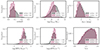 |
Fig. 1. Main physical properties used in our analysis. Panels above show spectroscopic redshift, stellar mass (log(Mstar/M⊙)), attenuation in the FUV band (AFUV), SFR and specific SFR (sSFR), both in logarithmic scale. The last bottom right panel shows the axis ratio (semi-minor/semi-major) from Meert et al. (2015). Black histograms represent distributions obtained from the whole sample of 29 487 galaxies (0.01 < z < 0.30), while maroon hatched histograms show distributions for the final sample used for the analysis (7986 galaxies). Legends show median values for all parameters calculated for the initial (black histograms) and final (maroon hatched histograms) samples. |
From the sample, we remove all galaxies with AFUV err larger than 0.25 [mag], as in the next step of our analysis, we want to bin galaxies regarding the AFUV value, and too large errorbars can influence our binning. The final sample, after this cut, contains 15 004 galaxies. We stress here that this cut has negligible influence on the main physical properties of the final sample, as shown in Fig. 1.
The number of objects in the sample drops above redshift z ∼ 0.1, which can be seen in the upper left panel in Fig. 1. A similar drop (but much steeper) can be seen below redshift 0.025. In Fig. 2, we check the AFUV distribution as a function of redshift. This figure shows that below redshift 0.025 and above redshift 0.1, the values of AFUV are not spread across the full range of this parameter. To obtain a representative sample of galaxies across the attenuation and redshift space range, we remove all galaxies with AFUV below the 1st (0.67 mag) and above the 99th (3.71 mag) percentile of the distribution. Moreover, we introduce additional cuts in redshift, removing galaxies outside the 0.025 and 0.1 redshift bin. Those two cuts allow us to keep a statistically significant galaxy sample characterised by an almost complete distribution of AFUV. Therefore, we decide to use in the following analysis only galaxies within the redshift range 0.025 < z < 0.1 (which reduces the sample to 9837 galaxies), and with 0.67 < AFUV < 3.71 mag, further reducing the sample to 9641 galaxies.
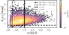 |
Fig. 2. Attenuation in the FUV band (AFUV) as a function of redshift. Two horizontal lines, dashed and dotted, represent the 1st and the 99th percentile of the AFUV distribution, respectively. The solid vertical line indicates redshift equal to 0.1, while the dashed double-dotted line represents a redshift cut at 0.025. Above that redshift line, the sample cannot probe the most extreme AFUV values. |
As the last step of the sample selection, we remove all galaxies in the tail of the sSFR distribution. From the SDSS distribution, we remove the tail of the main sequence distribution by selecting only galaxies located within 4σ of the sSFR distribution (i.e. −10.34 < log(sSFR/yr−1) < − 9.49, as illustrated in Fig. 3). This cut removes 1655 objects.
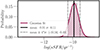 |
Fig. 3. Distribution of log(sSFR/yr−1) for the selected 7 986 galaxies in the redshift range 0.025 < z < 0.1. A vertical solid line and two vertical dotted lines represent the mean value of sSFR of the sample, and the mean value of the sSFR decreased/increased by 4σ of the distribution, respectively. |
Distributions of the main parameters used in the analysis are shown in Fig. 1. The full sample of 29 487 galaxies, without our internal cuts, is shown in black histograms, while the final sample of 7986 galaxies is presented as maroon-hatched histograms. The AFUV distribution, together with the Mstar distribution, show that cuts based on the AFUV err, redshift, AFUV and sSFR, do not change the main properties of the key physical properties, but only remove the most massive and in the same time the most active in the star formation processes, and the most attenuated galaxies.
3.5. Surface brightness calculation
For the final sample of 7986 galaxies, we calculate the surface brightness in each of the SDSS bands using the equation:
 (1)
(1)
where x stands for u, g, r and i band, mag for Petrosian magnitude and r for circular Petrosian radius. We note that we use the Petrosian radius for the surface brightness measurements, unlike the half-light radius, which is generally used in the literature (e.g. Paudel et al. 2017; Pérez-Montaño et al. 2022). As we do not have a half-light radius measurement for all the photometric bands used in this work, we chose to adopt the Petrosian radius in all the bands for consistency (Meert et al. 2015, 2016 provides half-light radius measurements only for the g, r and i bands, without the u-band). Graham et al. (2005) shows that the Petrosian radius for a galaxy with Sérsic index n = 1 (which is a reasonable assumption for the main-sequence galaxies studied in this work) is about twice larger than its Sérsic half-light radius. This will result in our surface brightness measurements ∼1.5 mag arcsec−2 fainter than those estimated using the half-light radii. However, such a systematic offset does not affect any of the trends studied in this work. Therefore, from here upon, we adopt the surface brightness measurements obtained using the Petrosian quantities.
We apply the correction for inclination (following Zhong et al. 2008; Pahwa & Saha 2018):
 (2)
(2)
where b/a represents the ratio of a galaxy’s minor and major axis. From now on, we always use only ‘corrected’ surface brightness in the analysis, and thus we drop the subscript corrected from the definition of μx, corr. Figure A.1 shows the distribution of the magnitudes and calculated surface brightness based on the Eqs. (1) and (2) for the final sample used in the analysis.
3.6. AFUV– LSST-like observables relations
We look for possible relations between observed LSST-like data (fluxes, magnitudes, colours, surface brightness in different bands, as well as the ratio between different surface brightness) in four SDSS bands (u, g, r, and i) and the attenuation in the FUV band estimated via fitting the UV to IR SED. The AFUV relation with colours and surface brightness calculated in different bands are presented in Appendix C. We also tried to use colours, but the relations are too narrow to separate different attenuation levels. GSWLC-X2 AFUV values were obtained using GALEX, SDSS, and WISE photometry calibrated on the Hershel ATLAS (Salim et al. 2018), ensuring proper dust attenuation estimation. The method used by Salim et al. (2018) combined SED constrained with CIGALE (Burgarella et al. 2005; Noll et al. 2009; Boquien et al. 2019) fitting code with infrared luminosity (SED+LTIR fitting; more details can be found in Salim et al. 2018). Our main goal is to find a simple proxy for AFUV based on the observational LSST-like data.
We checked all possible relations between colours, magnitudes, surface brightnesses, and their ratios. As a result, we find a promising relation between (u−r) colour, the surface brightness calculated in the u band, and the AFUV, which is characterised by a monotonic rise of the ratio of (u−r) colour and the u surface brightness with the AFUV values, and an extensive parameter locus (more than 0.6 mag in colour; for example, the (g − i) colour gives only ∼0.3 mag width, which makes the AFUV analysis more complicated taking into account the uncertainties of photometric measurements, and so forth). We also find a very similar relation using (u−i) instead of (u−r). The two main changes between both relations (the chosen one (u−r)–μu–AFUV and the second best one (u−i)–μu–AFUV) are the larger global slope uncertainty for (u−i) shown in Fig. C.1, and larger uncertainties for the final AFUVp equation based on larger errors for the intercept equation (Eq. (3)). The (u−r) or (u−i) colour is a natural indicator of dust attenuation since dust affects the slope of the galaxy SED. Both colours also cover the Balmer break, so they are very good indicators of the age of the stellar population. We are aware that we have a degeneracy between age and dust attenuation; since we have no information on the ages of the GSWLC and a very narrow redshift range, we subsequently analyse this degeneracy in the forthcoming analysis using much smaller but more informative, reference catalogues. The surface brightness in the band closest to UV SDSS is an indicator of the SFR as it traces light from the young stellar populations. The combination of these two parameters can be thus expected to be sensitive to dust attenuation for young stellar populations. However, this is the first time, to our knowledge, that these parameters have been combined to derive the proxy for AFUV. In Sects. 4 and 5, we present and analyse this relation in detail.
4. AFUV prior: (u−r) colour versus surface brightness in the u band
To study the relation between the colour and the surface brightness, we divide our sample into 14 AFUV bins to check if different attenuation values follow different relations in the colour − surface brightness space and if they can be separated. These bins are presented in Table 2 and graphically shown in Fig. 4. Each bin contains at least one percent of the final sample (at least 70 galaxies). Due to small numbers of galaxies in the GSWLC-X2 having AFUV lower than 1 mag, we use a variable bin width to probe as densely as possible the lowest attenuation range, which is underrepresented in the catalogue. Thus, the first bin has a width of 0.05 mag, the second is 0.10 mag wide, and the third is 0.15 mag wide. Starting from the fourth, the width is greater at 0.20 mag. Additionally, to increase the number of galaxies in each bin, as well as to include possible uncertainties arising from the redshift estimation or physical properties, we add overlaps between bins. These overlaps increase with increasing AFUV according to the relation: binn⋅0.005, where binn refers to the bin number. This helps us to gather enough galaxies in the less populated bins of high AFUV (larger than 2 mag), but also to take into account the uncertainties of the AFUV estimated by Salim et al. (2018), as for larger AFUV we also have larger AFUV err (it can be seen later in the right bottom panel of Fig. 7, blue circles).
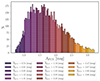 |
Fig. 4. Distribution of AFUV for the final sample of 7814 main sequence galaxies in the redshift range 0.025 − 0.1. The palette of colours represents the AFUV bins used in our analysis. The mean AFUV value for each bin ( |

We perform a linear fit in each AFUV bin in the (u−r)–μu parameter space, as this relation shows the most prominent slope of the general relation (0.0796 ± 0.0024)4, Appendix C. Moreover, the (u−r) colour space is wide enough to separate different attenuation levels, taking into account measurement errors for future LSST observations. Since the μu range is much wider than the range of (u−r), and more often is contaminated by outliers caused by uncertainties in calculating Petrosian radii and Pertosian magnitudes, we perform the fit only between the 10th and the 90th percentile of the μu distribution in each bin. Figure D.1 shows fits of the relation (u−r) versus μu fits for all AFUV bins, while Fig. 5 presents combined linear fits for all 14 bins. In Fig. 5, it is evident that for all AFUV bins, the (u−r)–μu relation maintains a consistent slope, with the intercept gradually increasing as AFUV rises. We have interpreted the flattening observed in the lowest and highest AFUV values as being related to the much less densely populated part of our sample. This can be seen in Table 2 and Fig. 4, where AFUV values lower than ∼0.8 mag and greater than 2.7 mag constitute only about 8% of the total sample analysed in our manuscript. Figure A.2 shows the same relation between (u−r) − μu and AFUV, but with an additional background of galaxies used in our analysis colour − coded according to the value of AFUV, and with the interpolated linear fit with μu in a range of 22.5 − 27.5 [mag arcsec−2]. For the simplicity in the main manuscript, we show only fits with the ±1σ uncertainty around estimated lines.
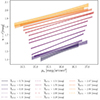 |
Fig. 5. Relations fitted between observed (u−r) colours and μu for 14 AFUV bins. The sequence of colours represents the one used for AFUV bin in Fig. 4. Filled areas display the ±1σ uncertainty around estimated lines. |
4.1. Global (u−r) – μu – AFUV relation
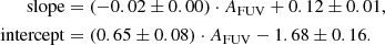
Figures 5 and A.2 indicate that there is a possibility to create a global relation between observed (u−r) colour, surface brightness in the u band and the attenuation in the FUV band. To find a relation, we examine the slopes and the intercepts of the relation between (u−r) and μu for each AFUV bin. We show in Fig. 6, a relation between both slopes and intercepts as a function of AFUV, together with two linear fits: one for the slopes and one for the intercepts, both as a function of AFUV:
 (3)
(3)
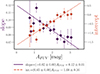 |
Fig. 6. Slopes and intercept from (u−r)–μu fits. Interpolated slopes (left axis) and intercepts (right axis) obtained from linear fits for all 14 bins of AFUV (Fig. D.1), as a function of AFUV. The left axis represents slopes (purple full diamonds), and the right axis represents intercepts (red full circles). Linear fits and associated fitted parameters are presented using dashed-dotted lines for slopes and dashed lines for intercepts. |
The increase in scatter for slope ad intercept with decreasing AFUV can be explained by smaller bin sizes and less representative samples in the global distribution of AFUV.
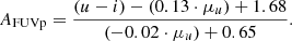
We derived a solution for this set of two equations based on the fitted relations (slopes and intercepts with respect to AFUV shown in Eq. (3)), resulting in a linear expression that characterises AFUV through the combination of (u−r) and μu. This final relation (Eq. 4) incorporates all three values: two entirely observational ((u−r) and μu) and one physical property (AFUV) obtained from the SED fitting from GSWLC:
 (4)
(4)
This equation provides a proxy for the AFUV when only optical measurements (fluxes and radii) are available, as will be the case for the majority of the LSST survey5 This proxy can significantly shorten the time needed to estimate all physical parameters through the SED fitting, as the grid for the dust attenuation properties can be much narrower and more specific.
We have also checked that using half-light instead of Petrosian radii will not change our relation significantly. Using approximately ∼1.5 mag arcsec−2 brighter values of surface brightness (see Sect. 3.5) results in changes of two values from Eq. (4): from 1.68 to 2.50 and from 0.65 to 0.74. This change results in the mean difference between AFUVp obtained with Petrosian end effective values equal to 0.05 [mag], with σ = 0.45 [mag].
Future LSST observations will provide more precise magnitude and morphology measurements than the data employed in this manuscript, where we adopt Petrosian radii and magnitudes from SDSS DR12. We plan to perform a similar test for the data acquired from LSST Deep Drilling Fields to better calibrate Eq. (4) as soon as the observations, both optical from LSST and from other ground-based and satellite observatories are collected. For those fields, near-IR data will also be available, for example, VISTA-NIR, which will further help us to constrain reliable dust properties, including attenuation in the FUV band in the broader AFUV range. LSST will enable the investigation of the lower AFUV range, since a substantial percentage of galaxies observed by LSST will be LSB galaxies. While low in comparison to many other types of galaxy, FUV attenuation levels among LSB galaxies are still non-negligible (i.e. AFUV < SPSDOUBLEDOLLAR > < 0.4 mag), as shown recently by Junais et al. (2023). While waiting for observations and estimates of the main physical properties of galaxies from the Deep Drilling Field, we can use Eq. (4) to calculate a proxy representing dust attenuation for star-forming galaxies. This relation will be used to prepare a software pipeline to estimate physical properties from future LSST data by members of the LSST Galaxy Science Collaboration (Robertson et al. 2017).
4.2. Final AFUV prior
The final distribution of the obtained AFUVp, as well as the comparison with AFUV from the original work of Salim et al. (2018), is shown in Fig. 7. Panel a in this figure shows the AFUV and AFUVp distributions. It is clearly seen that the distributions are different and that the prior obtained from (u−r) and μu can reach both much lower (to the AFUVp = 0 mag) and larger (up to AFUVp > 4 mag) values than the original AFUV from Salim et al. (2018). The Kolmogorov–Smirnov test, which is a commonly used non-parametric test based on the distance between two cumulative distributions, confirms that AFUV and AFUVp do not come from the same distribution (pKS = 1.11 × 10−128). For this plot, we have removed 426 galaxies for which the value of AFUVp from Eq. (4) is less than 0. All galaxies from the removed sample occupy (u−r)–μu loci not included in our analysis (just below the bin with the lowest value of mean AFUV ( [mag])). Figure B.1 shows the position of all 426 galaxies in the (u−r)–μu plane.
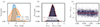 |
Fig. 7. Main properties of obtained AFUV priors. Panel a shows the distributions of original AFUV from the Salim et al. (2018) work obtained from careful SED fitting based on measurements from UV to mid-IR (AFUV, blue left hatched histogram), and AFUVp calculated based on Eq. (4) (orange right hatched histogram). Panel b presents the distribution of the difference between AFUV and AFUVp and denotes its median value. In panel c, the difference between AFUV and AFUVp is shown as a function of redshift. We removed for clarity from panel a 426 galaxies, for which calculated AFUVp was lower than 0. |
We notice here the sharp cut in the low-end of the AFUV distribution (visible also in Fig. 1, right upper panel). It can be related to the specific sets of parameters used in Salim et al. (2018) or the data set for which the SED fitting was performed. As shown in Osborne et al. (2023), the GALEX data, which give direct insight into the young stellar population and were used to create GSWLC, are partially affected by blending. The new catalogue built with a new software pipeline EMphot, which uses forced photometry from the SDSS catalogue, presented by Osborne et al. (2023), revealed that magnitudes used in GSWLC were systematically fainter (up to 0.5 mag) due to insufficient background subtraction for faint sources. The new, deblended, GALEX catalogue of Osborne et al. (2023) shows that ∼15% of galaxies in the GSWLC catalogue were moderately affected by blending (contamination > 0.2 mag), and 2.4% of galaxies were contaminated at the level of more than 1 mag. To summarise, the NUV and FUV GALEX magnitudes originally used to estimate AFUV by Salim et al. (2018) were fainter than the corrected deblended magnitudes, but only a small percentage of galaxies in our sample can be affected by this effect. It means that GALEX data used by Salim et al. (2016) has negligible influence on the lack of low AFUV values in the original GSWLC-X2 catalogue for the main sequence galaxies6.
The mean difference between AFUV and AFUVp equals 0.01 mag, with a σ = 0.74 mag (see middle panel of Fig. 7). From hereupon, we use this σ, which is the scatter in the difference between fiducial values of AFUV and AFUVp, as a constant uncertainty for our estimated AFUVp (hereafter: AFUVp err). We want to stress that, in the future, with the LSST-like observations, it will also be possible to calculate the AFUVp err directly for individual sources based on the uncertainties in the observed colour, surface brightness, and the fit coefficients shown in Eq. (4). However, we are currently restricted to a limited number of galaxies, which affects the uncertainties of our fits from Eq. (3). Additionally, we have significant photometric errors (for both radii and magnitudes). Furthermore, the fiducial AFUV is not free of uncertainties (limited to AFUV err < 0.25 mag, based on our selection in Table 3). Therefore, for the simplicity of this work and to avoid significant overestimations of errors, we decided to use a constant uncertainty of AFUVp err = 0.74 mag.
Input parameters for the code CIGALE.
We do not observe any redshift dependence (panel c, Fig. 7); however, the redshift range used in this analysis is very narrow (0.025–0.100). We can reasonably expect that the much deeper LSST data will require adding a redshift-dependent calibration.
The obtained priors do not follow a 1:1 relation with the AFUV values calculated directly from fits to the UV-IR range SED. This is due to many reasons, where the most important ones are (1) uncertainties of the original AFUV, (u−r) and μu, which were not taken into account when constructing the (u−r) − μu − AFUV relation; (2) the quality of the SED fits obtained by Salim et al. (2018; our only selection is based on REDCHISQ < 5); (3) the quality of the data used for full fitting – there is no information about the signal-to-noise ratio for specific bands or the goodness of the measurement; (4) but even more importantly, the (u−r)μu relation is not tight as the (u−r) colour depends both on the age of the stellar population and on the dust. Nevertheless, the median difference between AFUV obtained based on the careful fitting of broadband photometry from UV to IR and AFUVp determined from (u−r) and μu observed quantities is only 0.10 mag larger than the median AFUVp err (0.12 mag).
5. Reliability of AFUVp derived from LSST-like observations
Even if, as mentioned above, the agreement between AFUVp ± AFUVp err and AFUV estimated via SED fitting by Salim et al. (2016, 2018) is not perfect, the correlation is evident, and the advantages of such an approach are numerous. An AFUV prior obtained from an optical-only dataset (without any information about dust emission or proxy from UV observations) can help to reduce the number of parameters needed to estimate the main physical properties of studied galaxies. It can also reduce the risk of overfitting by decreasing the number of free parameters used for SED fitting based on five optical broadbands only.
To check whether the obtained AFUVp values can lead to reliable estimates of the main physical properties of galaxies, we perform a set of tests using only optical broadband data with and without two priors: the original AFUV from GSWLC obtained by Salim et al. (2018), which we call now AFUVs (and AFUVs err) to distinguish between both AFUV values used in the test, and the AFUVp (and AFUVp err) from Eq. (4).
To test using AFUVp obtained via Eq. (4) as a prior, we perform six CIGALE runs to fit the SED of our sample. We use SDSS DR 12 ugriz measurements from Alam et al. (2015) (in case of Salim et al. 2016, 2018, they used SDSS DR10). Salim et al. (2016, 2018) made use of additional data from GALEX and WISE which are not taken into account in our analysis. A simple run based on five optical bands only is intended to reproduce the future LSST-like observations (without the LSSTy band). We employ the same SED fitting code as used for the GSWLC data set. Parameters and modules used are described in Table 3. As our SED coverage consists of only five optical SDSS data points, we do not include any dust emission module.
We categorise the SED fitting parameters into two main groups: FULL–run (based on the description given by Salim et al. 2016, 2018) and LIGHT–run, with a significantly reduced number of parameters describing dust attenuation and the age of the late burst for the star formation history module (details are listed in Table 3). Runs based on FULL–run parameters produce 332 640 templates per redshift bin. In contrast, utilising LIGHT–run parameters reduces the number of templates to only 5540 per redshift bin. Thus, the number of generated templates decreases by 98%. We performed our runs for 7934 galaxies using Intel Core i9–9900K CPU @ 3.60 GHz processor with 64 GB memory and 8 cores (16 threads). FULL–run required 188 seconds to compute models while the LIGHT–run did the same in 11 s. The Bayesian estimates of the physical properties for these templates for the FULL–run CIGALE took 203 s, while for the LIGHT–run, only one second. Thus, both runs used the same time to estimate best-fit properties for all galaxies (85 s). Thus, the LIGHT–run required only 3% of the time spent on the FULL–run. This reduction in the number of templates is of particular significance for ‘big data’ galaxy samples like the LSST. For LSST-like surveys, with billions of observed galaxies, running full, detailed SED fitting will be impossible due to CPU and memory limitations.
We used the LSST-like data set, and we performed the SED fitting using FULL–run and LIGHT–run parameter sets. For FULL–run and LIGHT–run parameters we further divide runs into three groups: (1) without any priors (tagged as NO prior), without any indication of a preferable AFUV value, (2) with the AFUVs err and AFUVs err used as priors for the CIGALE run, and (3) with AFUVp and AFUVp err. To add priors, we used the properties option from the original CIGALE tool7, while for runs without priors, we left the properties option empty. Runs with and without priors still need to be supported by the input parameters for the dust attenuation module. In all six cases, we used input parameters as listed in Table 3.
In Fig. 8, we present the difference between estimated Mstar and SFRs obtained via our six runs and the original (fiducial) values from the GSWLC catalogue. We stress that for all six runs, only u, g, r, i, and z SDSS broadband photometry was used. The resultant loci of the obtained six main sequences are shown in Fig. 9.
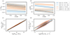 |
Fig. 8. Difference between SFR and Mstar from the original GSWLC catalogue (Salim et al. 2018), and those obtained in this work. The difference ΔMstar was calculated as log(Mstar this work/Mstar); and ΔSFR was obtained in an analogous way. Panels a and b show the difference in the stellar masses and SFRs, correspondingly, as a function of redshift, with shaded areas represent standard deviation of the scatter; panels c and d present the relation between the fiducial values and the estimates obtained in this work, with contours showing the distribution of the data. Runs based on GSWLC set of parameters, FULL–run, are shown in blue-coloured lines, while those obtained from LIGHT–run – in an orange-coloured set of lines. Black solid lines visible in panels c and d represent 1:1 relations. |
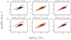 |
Fig. 9. Comparison of physical properties obtained in FULL–run, and LIGHT–run runs. Upper panels present results obtained based on FULL–run parameter sets (332 640 templates per redshift bin), while the results shown in bottom panels were estimated based on the LIGHT–run sets of parameters (5544 templates per redshift bin). Black contours shown in each panel correspond to fiducial values from the GSWLC-X2 catalogue (SFR, Mstar), while orange contours illustrate physical parameters estimated in this work. The left column presents results obtained without priors, the middle column – with AFUVs from the GSWLC catalogue, and the right column – with AFUVp calculated from Eq. (4). |
It is important to note that processing LIGHT–run data with CIGALE without AFUV prior leads to large overestimates of the SFR (see also Riccio et al. 2021). Priors, even if based only on optical measurements, can reproduce the physical parameters of the fiducials well enough. Moreover, priors can also help to reduce the number of parameters, and hence the CPU time, required to analyse large numbers of galaxies.
6. Discussion
Figures 8 and 9 show the differences between the original (fiducial) physical parameters from the GSWLC catalogue and the physical parameters obtained with two sets of parameters: FULL–run, and highly reduced LIGHT–run. Additionally, different AFUV priors (and also no prior for even more detailed comparison) were applied in these runs. Table 4 shows the mean SFR and the mean Mstar accompanied by their uncertainties for fiducial parameters from the GSWLC and those obtained from six additional runs described in Sect. 5.
6.1. Influence of the AFUVp or lack of it on the Mstar estimation for the LSST-like observations
Results presented in Figs. 8a,c, show a negligible, ≤0.1 dex, difference in the estimated Mstar between all six runs and the original Mstar from the GSWLC catalogue. The consistency in the estimations is actually expected given the complete set of the SDSS DR 12 optical broadband data used by Salim et al. (2018) and in our work. Detailed coverage of the optical spectrum, from u to z bands, allows reconstruction of the old stellar population in the galaxy (especially at low redshift), which is the main ingredient of the total stellar mass of both quiescent and normal star-forming galaxies.
However, it is worth mentioning that only for runs without prior ΔMstar, defined as log(Mstar this work/Mstar), is lower than −0.07, and monotonically decreases with redshift. It implies that for optical data only, without any proxy for dust emission or AFUV, the Bayesian method of estimating physical parameters prefers to choose templates corresponding to somewhat less massive galaxies. It is clearly visible when comparing runs without priors: for the run with a larger number of templates (marked as FULL–run) ΔMstar is systematically shifted towards lower values of Mstar when compared to the LIGHT–run. We want to stress here that this effect can be caused by overfitting (it can be seen also Fig. 7 in Riccio et al. 2021, where the Mstar is very slightly, but still overestimated due to the number of used templates). The number of parameters used in Salim et al. (2018) was allowed thanks to a larger number of measurements available, which is not the case in the LSST-like dataset. We stress that possible overfitting should be avoided for the LSST-like data analysis, as it may cause the choice of templates of systematically less massive galaxies, which is another reason why introducing a prior to reduce the size of the parameter grid is needed.
6.2. Influence of the AFUVp and lack of the prior on the SFR estimation for the LSST-like observations
In this section, we check how the use of priors influences the estimations of the SFR. Again, we calculate the ratio between the fiducial physical value from GSWLC catalogue and those obtained in our runs. We define this ratio, ΔSFR, as log(SFRthis work/SFR). The results are shown in Figs. 8b,d.
6.2.1. No AFUV prior involved
The first conclusion from this test, presented in the right panels of Fig. 8, is that using optical data only without any prior (that is, without giving any values for the properties option, see note 7) for the dust attenuation results in a significant overestimation of the SFR, which decreases with redshift. The same overestimation and its redshift dependence were found by Riccio et al. (2021) for a sample of ∼50 000 main sequence galaxies. They used a sample of observed galaxies to estimate the expected LSST fluxes in the ugrizy bands and then performed SED fitting. They found that the Mstar remains well estimated (similarly to our result shown in Sect. 6.1) by the LSST–like data set. However, at the same time, the SFR and the dust luminosity are overestimated when the LSST–like sample alone is used. The SFR overestimation found by Riccio et al. (2021) is redshift dependent and clearly decreases with redshift, disappearing at about redshift ∼1. This effect can be explained by the wavelength range of the LSST observations. At redshift ∼0 LSST probes mainly old stellar population, without any band probing young stellar population or dust properties. As redshift increases, the LSSTugriz filters start to cover the UV rest frame, and the estimates of the SFR significantly improve.
The lack of information about the UV and MIR rest-frame wavelengths for the LSST low redshift sample causes a large overestimation of the attenuation during the fitting (Riccio et al. 2021), which then translates into an overestimation of the dust luminosity and, finally, the SFR. As shown in Fig. 8, both FULL–run and LIGHT–run sets of parameters, applied without any AFUV prior (blue and orange solid lines, respectively), result in significant SFR overestimation: mean ΔSFR for FULL–run and LIGHT–run runs without priors equal to 0.34 and 0.48, respectively. Based on Eq. (1) from Riccio et al. (2021), that is, ΔSFR = SFRLSST/SFRUV-FIR, the expected ΔSFR at redshift 0.062 (which is the mean redshift of our galaxy sample) is equal to ∼0.5. As seen from panels b and d of Fig. 8, our results, although limited to a much narrower redshift range, are in agreement with predictions of Riccio et al. (2021).
We stress that enlarging the parameter space in the SED fitting process, with only a stellar population as a proxy, cannot solve the problem of the overestimation of SFR. This conclusion is illustrated in Fig. 9. In this figure, the black contours are based on the original catalogue of Salim et al. (2018), while the orange contours show the estimates used in this work. It is clearly seen that runs based on the optical data only without any priors result in a significant systematic overestimation of SFR (panels a and b). The overestimation occurs both for the FULL–run and the LIGHT–run parameter grid. The overestimation of the SFR results in a shift of the main sequence locus and can affect not only directly the physical analysis but also the classification of normal star-forming and starbursting galaxies. Such classification can propagate through the statistical analysis of evolutionary paths and many other science cases.
6.2.2. Overcoming SFR overestimation with AFUV and AFUVp
In Riccio et al. (2021), it was also found that the Mstar–AFUV prior can solve the SFR overestimation for objects without UV or IR observation. As seen in the panel b of Fig. 8, SFR estimated with AFUV priors (both FULL–run and LIGHT–run) are much closer to the fiducial values than the SFR obtained without any priors. The ΔSFR for runs with priors are lower than 0.1.
The quality of SFR reconstruction can be seen in the central and the right columns in Fig. 9. Adding AFUV prior (original AFUVs from GSWLC catalogue or AFUVp from Eq. (4)) clearly reduces the overestimation. The calculated SFR ratio between mean fiducial values from Salim et al. (2018) and those obtained in this work with AFUVs prior is less than 0.05, and with AFUVp – less than 0.1.
OriginalAFUVprior. Results presented as blue and orange dashed lines (FULL–run and LIGHT–run, respectively) in Fig. 8 are based on the AFUVs prior. Although the difference with respect to the fiducial SFR values is almost negligible (ΔSFR = 0.1), the relation is not 1:1 (which would correspond to ΔSFR = 0). In both cases, FULL–run and LIGHT–run sets of parameters, the difference with respect to the fiducial value of SFR, ΔSFR, decreases with redshift.
This small difference results from a narrower wavelength coverage than used by Salim et al. (2018). At the same time, these two runs demonstrate that AFUVs prior works almost equally well for the dense (FULL–run) and significantly reduced (LIGHT–run) grids of parameters.
The central panels in Figs. 9c,d show the main sequence built using the original AFUVs prior for FULL–run (panel c) and LIGHT–run (panel d) runs. The original main sequence from the GSWLC catalogue is below the orange contours. These two panels show that the use of the original AFUVs prior reproduces the fiducial values of the SFR equally well with fewer parameters (we remind that the number of templates in the LIGHT–run case is 98% lower than in the FULL–run case).
Of course, without ancillary data from other facilities, the actual value of AFUV will be unknown for most of LSST galaxies. The purpose of this test was to demonstrate that (1) providing an AFUV prior is instrumental in the recovery of SFR and (2) that an AFUV prior can be used along with a small number of free parameters in the fitting process, which will reduce the risks of overfitting in the case of a low number of data points. However, galaxies at redshifts higher than ∼2 will benefit from the restframe FUV observations with the u band of LSST. This will give unprecedented power for probing the attenuation in this band specifically. Therefore, attenuation in FUV can be used as a prior for high redshift galaxies, correcting their SFR and Mstar estimations when IR data are missing.
Results based on theAFUVpfrom (u-r)–μurelation. To test the effect of the prior obtained from Eq. (4), we run FULL–run and LIGHT–run setup of parameters with AFUVp. SFRs obtained from this test are shown with blue and orange dotted lines (FULL–run, and LIGHT–run, respectively) in panels b and d of Fig. 8. Both results are very close to the fiducial values (ΔSFR < 0.1, very similar to the results obtained with an original prior estimated from full UV–IR SED fitting, Salim et al. 2018). The FULL–run parameter setup with an AFUVp provides values of SFR which have a small bias almost uniform along all the probed ranges of the SFR, with both mean and median ΔSFR equal to 0.11. In the run with a smaller grid of parameters (LIGHT–run+AFUVp), a similar small bias is observed (the median and the mean ΔSFR = 0.09). This small overestimation rises somewhat with redshift.
The right column of Figs. 9e,f shows the comparison of the main sequences of 7934 galaxies based on physical properties obtained from the original GSWLC catalogue and those calculated using AFUVp from Eq. (4). It can be seen that for the case of a large number of parameters (FULL–run, panel e) and a much smaller number of templates (LIGHT–run, panel f), the obtained main sequence is narrower than the original one, and the overestimation can be seen for more massive galaxies. The obtained main sequence is, however, much closer to the fiducial one than in the case of fitting with no priors. We emphasize that this may be related to a lower fraction of massive galaxies in our sample (see Fig. 1) but also to the representative original AFUVs estimates, which have not been taken into account in our fit of the slopes–intercepts.
The linear relations found between μu and the (u−r) colours for all theAFUV bins show that the morphological aspect of galaxies might be an indicator of attenuation. Surface brightness encodes in itself the spatial extent of galaxies, and indications of a correlation between the amount of attenuation on the one hand and the compactness of galaxies on the other hand were found in Buat et al. (2019), Hamed et al. (2023a,b). The μu can also be correlated with the age of stellar populations, and so it helps to break the degeneracy of the (u−r) colour (which depends both on the dust attenuation and the stellar population age).
We conclude that the LIGHT–run+AFUVp run results in only the small effect of SFR overestimation, visible mainly for massive galaxies. For the case of the optical SDSS data only, the reduced number of templates and AFUVp created based on (u−r) colour and μu are thus optimal, although not perfect, solutions to reproduce the main physical properties of galaxies even without IR or UV data.
7. Summary
In this work, we aimed at constructing the proxy of dust attenuation in the FUV wavelength range from the optical photometric LSST-like data only. To imitate the LSST optical detections of low redshift main-sequence galaxies, we used SDSS observations. Furthermore, for the analysis of the dust attenuation, we selected only galaxies with IR auxiliary observations, with homogeneous data analysis and estimated main physical parameters, such as Mstar, SFR and AFUV. We selected a sample of 7934 local (0.025 < z < 0.1) main-sequence star-forming SDSS galaxies with properties previously measured based on multiwavelength IR-to-UV photometric data. We used the GSWLC catalogue of physical properties citepSalim2018 together with their SDSS DR 12 ugriz measurements (Alam et al. 2015) and inclination from citeMeert2015MNRAS.446.3943M. We calculated their surface brightness in the ugri bands and corrected for inclination and cosmological surface brightness dimming.
We tested different setups of the CIGALE SED fitting code in order to find an optimal method to estimate the main physical properties of galaxies when only the ugriz photometric data are available. Our results can be summarised as follows:
-
We find that the proxy for dust attenuation, AFUVp, can be constructed based on the combination of the (u−r) colour and the galaxy surface brightness in the u band (μu). The formula is given by Eq. (4). The formula remains almost the same if the colour (u−i) is used instead of (u−r), Eq. (5) in the footnote.
-
Surface brightness measured in bands other than u do not provide an equally good estimate for AFUV, as it can be seen in Fig. C.1.
-
The Mstar can be well recovered by the SED fitting in the optical range only, with no necessity to use additional priors.
-
The SFR cannot be well measured based on the SED fitting method in the optical range only due to missing information about dust attenuation. In the case of CIGALE, it results in systematic and redshift-dependent overestimation of SFR at the level of ΔSFR > 0.3 dex, which is in agreement with the findings of Riccio et al. (2021).
-
The SFR can be recovered almost unbiased, with ΔSFR < 0.05 dex, if the fitting is performed with an AFUV proxy. However, such a proxy will not be available for all future LSST data without auxiliary data.
-
The AFUVp given by Eq. (4), used as a proxy for the SED fitting, allows for very good recovery of SFR with only a small bias ΔSFR ∼ 0.1 dex.
-
This bias is both Mstar and redshift dependent, which implies that the AFUVp proposed in Eq. (4) in the future will have to be refined and generalised based on the calibration with deeper data and larger galaxy samples.
Additionally, we have found that when a prior for dust attenuation is used, the parameter grid used by the fitting code can be significantly reduced in order to avoid overfitting, which, in particular, tends to lead to overestimation of SFR. Also, thanks to the reduction of the number of generated templates by ∼98%, we decrease the computing time needed for fitting by a comparable factor, which will be of great importance for the ‘big data’ analysis of the LSST data.
Thus, this work proposes a strategy based only on optical photometric measurements to reliably and efficiently measure galaxy physical properties through SED fitting in future large surveys. The next steps will include the analyses based on galaxy samples deeper than the SDSS, complemented by the state-of-the-art simulations, which will allow for extensions of the proposed strategy towards higher redshift and lower brightness data sets, as well as cover different types of galaxies, which will likely require a diversified approach.
There are no Petrosian radii and magnitudes for the z band in this catalogue.
The detailed description of all SDSS flags can be found at https://www.sdss.org/dr12/algorithms/flags_detail/
The second most prominent relation is (u−i)–μu with slope 0.0799 ± 0.0047, however, the slope uncertainty is almost twice larger than for the slope uncertainty of the (u−r)–μu plane.
As discussed above, we obtained a very similar result for the (u−i)–μu plane:
 (5)
(5)
The main difference between equations are the larger uncertainties for slopes and intercepts in Eq. (3).
Based on private communication with S. Salim, we have found that the AFUV distributions based on the previous GALEX data used for the GSWLC catalogue and the AFUV obtained with the new, deblended GALEX measurements from Osborne et al. (2023) have a statistically negligible change.
To run CIGALE with the properties option, one has to add to the initial input file additional columns filled with prior values and corresponding errors. In the case of this work, we added two columns: attenuation.AFUV and attenuation.AFUV_err, and we filled them with AFUVp from Eq. (4) and AFUVp err equal to 0.74 mag, respectively.
Acknowledgments
We acknowledge and thank the referee for a thorough and constructive report, which helped improve this work. This research was done as a part of the NCBJ’s In-kind Contributions to the Vera C. Rubin Observatory Legacy Survey of Space and Time POL-NCB-S3. This research was supported by the Polish National Science Centre grant UMO-2018/30/M/ST9/00757 and the Polish Ministry of Science and Higher Education grant DIR/WK/2018/12. K.M. and J. have been supported by the National Science Centre (UMO-2018/30/E/ST9/00082). This research was also partially supported by the ‘PHC POLONIUM’ programme (project number: 49136QB), funded by the French Ministry for Europe and Foreign Affairs, the French Ministry for Higher Education and Research and the Polish NAWA. The project is co-financed by the Polish National Agency for Academic Exchange (BPN/BFR/2022/1/00005). This research was supported by from COST Action CA21136 – ‘Addressing observational tensions in cosmology with systematics and fundamental physics (CosmoVerse)’, supported by COST (European Cooperation in Science and Technology). R.D. gratefully acknowledges support by the ANID BASAL project FB210003. M.B., C.S., and M.A. acknowledge support from the ANID through FONDECYT grants (no. 1211000, 11191125 and 1211951) and Agencia Nacional de Investigación y Desarrollo (ANID) BASAL project FB210003. D.D. acknowledges support from the National Science Center (NCN) grant SONATA (UMO-2020/39/D/ST9/00720). J.R.M. is supported by STFC funding for UK participation in LSST, through grant ST/Y00292X/1. A.N. and M.R. acknowledge support from the Narodowe Centrum Nauki (UMO- 2020/38/E/ST9/00077), and M.R. also acknowledges support from the Foundation for Polish Science (FNP) under the program START 063.2023. O.D. acknowledges support from the Programa de doctorado en Astrofísica y Astroinformática of Universidad de Antofagasta. W.J.P. has been supported by the Polish National Science Center project UMO-2020/37/B/ST9/00466. J.R. acknowledges funding from the University of La Laguna through the Margarita Salas Program from the Spanish Ministry of Universities ref. UNI/551/2021-May 26, and under the EU Next Generation. This work made use of Astropy (http://www.astropy.org): a community-developed core Python package and an ecosystem of tools and resources for astronomy (Astropy Collaboration 2013, 2018, 2022)
References
- Ahn, C. P., Alexandroff, R., Allende Prieto, C., et al. 2014, ApJS, 211, 17 [NASA ADS] [CrossRef] [Google Scholar]
- Alam, S., Albareti, F. D., Allende Prieto, C., et al. 2015, ApJS, 219, 12 [Google Scholar]
- Astropy Collaboration (Robitaille, T. P., et al.) 2013, A&A, 558, A33 [NASA ADS] [CrossRef] [EDP Sciences] [Google Scholar]
- Astropy Collaboration (Price-Whelan, A. M., et al.) 2018, AJ, 156, 123 [Google Scholar]
- Astropy Collaboration (Price-Whelan, A. M., et al.) 2022, ApJ, 935, 167 [NASA ADS] [CrossRef] [Google Scholar]
- Baldwin, J. A., Phillips, M. M., & Terlevich, R. 1981, PASP, 93, 5 [Google Scholar]
- Battisti, A. J., Calzetti, D., & Chary, R. R. 2016, ApJ, 818, 13 [NASA ADS] [CrossRef] [Google Scholar]
- Bianchi, L., Conti, A., & Shiao, B. 2014, Adv. Space Res., 53, 900 [Google Scholar]
- Bogdanoska, J., & Burgarella, D. 2020, MNRAS, 496, 5341 [NASA ADS] [CrossRef] [Google Scholar]
- Boquien, M., Burgarella, D., Roehlly, Y., et al. 2019, A&A, 622, A103 [NASA ADS] [CrossRef] [EDP Sciences] [Google Scholar]
- Boquien, M., Buat, V., Burgarella, D., et al. 2022, A&A, 663, A50 [NASA ADS] [CrossRef] [EDP Sciences] [Google Scholar]
- Brinchmann, J., Charlot, S., White, S. D. M., et al. 2004, MNRAS, 351, 1151 [Google Scholar]
- Brough, S., Collins, C., Demarco, R., et al. 2020, arXiv eprints [arXiv:2001.11067] [Google Scholar]
- Bruzual, G., & Charlot, S. 2003, MNRAS, 344, 1000 [NASA ADS] [CrossRef] [Google Scholar]
- Buat, V., Noll, S., Burgarella, D., et al. 2012, A&A, 545, A141 [NASA ADS] [CrossRef] [EDP Sciences] [Google Scholar]
- Buat, V., Heinis, S., Boquien, M., et al. 2014, A&A, 561, A39 [NASA ADS] [CrossRef] [EDP Sciences] [Google Scholar]
- Buat, V., Boquien, M., Małek, K., et al. 2018, A&A, 619, A135 [NASA ADS] [CrossRef] [EDP Sciences] [Google Scholar]
- Buat, V., Ciesla, L., Boquien, M., Małek, K., & Burgarella, D. 2019, A&A, 632, A79 [NASA ADS] [CrossRef] [EDP Sciences] [Google Scholar]
- Buat, V., Mountrichas, G., Yang, G., et al. 2021, A&A, 654, A93 [NASA ADS] [CrossRef] [EDP Sciences] [Google Scholar]
- Burgarella, D., Buat, V., & Iglesias-Páramo, J. 2005, MNRAS, 360, 1413 [NASA ADS] [CrossRef] [Google Scholar]
- Calzetti, D., Kinney, A. L., & Storchi-Bergmann, T. 1994, ApJ, 429, 582 [Google Scholar]
- Calzetti, D., Armus, L., Bohlin, R. C., et al. 2000, ApJ, 533, 682 [NASA ADS] [CrossRef] [Google Scholar]
- Chabrier, G. 2003, PASP, 115, 763 [Google Scholar]
- Charlot, S., & Fall, S. M. 2000, ApJ, 539, 718 [Google Scholar]
- Chary, R., & Elbaz, D. 2001, ApJ, 556, 562 [Google Scholar]
- Chevallard, J., Charlot, S., Wandelt, B., & Wild, V. 2013, MNRAS, 432, 2061 [CrossRef] [Google Scholar]
- Ciesla, L., Elbaz, D., Schreiber, C., Daddi, E., & Wang, T. 2018, A&A, 615, A61 [NASA ADS] [CrossRef] [EDP Sciences] [Google Scholar]
- Conroy, C. 2013, ARA&A, 51, 393 [NASA ADS] [CrossRef] [Google Scholar]
- Cortese, L., Ciesla, L., Boselli, A., et al. 2012, A&A, 540, A52 [NASA ADS] [CrossRef] [EDP Sciences] [Google Scholar]
- Dunne, L., Gomez, H. L., da Cunha, E., et al. 2011, MNRAS, 417, 1510 [NASA ADS] [CrossRef] [Google Scholar]
- Elbaz, D., Daddi, E., Le Borgne, D., et al. 2007, A&A, 468, 33 [NASA ADS] [CrossRef] [EDP Sciences] [Google Scholar]
- Gallazzi, A., Charlot, S., Brinchmann, J., White, S. D. M., & Tremonti, C. A. 2005, MNRAS, 362, 41 [Google Scholar]
- Galliano, F., Galametz, M., & Jones, A. P. 2018, ARA&A, 56, 673 [Google Scholar]
- Graham, A. W. 2001, MNRAS, 326, 543 [NASA ADS] [CrossRef] [Google Scholar]
- Graham, A. W., & de Blok, W. J. G. 2001, ApJ, 556, 177 [NASA ADS] [CrossRef] [Google Scholar]
- Graham, A. W., Driver, S. P., Petrosian, V., et al. 2005, AJ, 130, 1535 [NASA ADS] [CrossRef] [Google Scholar]
- Graham, A. W., Jarrett, T. H., & Cluver, M. E. 2024, MNRAS, 527, 10059 [Google Scholar]
- Hamed, M., Ciesla, L., Béthermin, M., et al. 2021, A&A, 646, A127 [NASA ADS] [CrossRef] [EDP Sciences] [Google Scholar]
- Hamed, M., Małek, K., Buat, V., et al. 2023a, A&A, 674, A99 [NASA ADS] [CrossRef] [EDP Sciences] [Google Scholar]
- Hamed, M., Pistis, F., Figueira, M., et al. 2023b, A&A, 679, A26 [NASA ADS] [CrossRef] [EDP Sciences] [Google Scholar]
- Harikane, Y., Ouchi, M., Inoue, A. K., et al. 2020, ApJ, 896, 93 [Google Scholar]
- Hurley, P. D., Oliver, S., Betancourt, M., et al. 2017, MNRAS, 464, 885 [Google Scholar]
- Ivezić, Ž., Kahn, S. M., Tyson, J. A., et al. 2019, ApJ, 873, 111 [Google Scholar]
- Jarrett, T. H., Chester, T., Cutri, R., et al. 2000, AJ, 119, 2498 [Google Scholar]
- Junais, Małek, K., Boissier, S., et al. 2023, A&A, 676, A41 [NASA ADS] [CrossRef] [EDP Sciences] [Google Scholar]
- Komatsu, E., Smith, K. M., Dunkley, J., et al. 2011, ApJS, 192, 18 [Google Scholar]
- Lang, D., Hogg, D. W., & Schlegel, D. J. 2016, AJ, 151, 36 [Google Scholar]
- Laureijs, R., Amiaux, J., Arduini, S., et al. 2011, arXiv e-prints [arXiv:1110.3193] [Google Scholar]
- Lo Faro, B., Buat, V., Roehlly, Y., et al. 2017, MNRAS, 472, 1372 [NASA ADS] [CrossRef] [Google Scholar]
- Małek, K., Buat, V., Roehlly, Y., et al. 2018, A&A, 620, A50 [Google Scholar]
- Meert, A., Vikram, V., & Bernardi, M. 2015, MNRAS, 446, 3943 [NASA ADS] [CrossRef] [Google Scholar]
- Meert, A., Vikram, V., & Bernardi, M. 2016, MNRAS, 455, 2440 [NASA ADS] [CrossRef] [Google Scholar]
- Meurer, G. R., Heckman, T. M., & Calzetti, D. 1999, ApJ, 521, 64 [Google Scholar]
- Noeske, K. G., Weiner, B. J., Faber, S. M., et al. 2007, ApJ, 660, L43 [CrossRef] [Google Scholar]
- Noll, S., Burgarella, D., Giovannoli, E., et al. 2009, A&A, 507, 1793 [NASA ADS] [CrossRef] [EDP Sciences] [Google Scholar]
- Osborne, C., Salim, S., Boquien, M., Dickinson, M., & Arnouts, S. 2023, ApJS, 268, 26 [NASA ADS] [CrossRef] [Google Scholar]
- Pahwa, I., & Saha, K. 2018, MNRAS, 478, 4657 [NASA ADS] [CrossRef] [Google Scholar]
- Paudel, S., Lisker, T., Huxor, A. P., & Ree, C. H. 2017, MNRAS, 465, 1950 [NASA ADS] [CrossRef] [Google Scholar]
- Pearson, W. J., Wang, L., van der Tak, F. F. S., et al. 2017, A&A, 603, A102 [NASA ADS] [CrossRef] [EDP Sciences] [Google Scholar]
- Pearson, W. J., Wang, L., Hurley, P. D., et al. 2018, A&A, 615, A146 [NASA ADS] [CrossRef] [EDP Sciences] [Google Scholar]
- Pearson, W. J., Pistis, F., Figueira, M., et al. 2023, A&A, 679, A35 [NASA ADS] [CrossRef] [EDP Sciences] [Google Scholar]
- Peek, J. E. G., & Schiminovich, D. 2013, ApJ, 771, 68 [NASA ADS] [CrossRef] [Google Scholar]
- Peng, C. Y., Ho, L. C., Impey, C. D., & Rix, H.-W. 2002, AJ, 124, 266 [Google Scholar]
- Pérez-Montaño, L. E., Rodriguez-Gomez, V., Cervantes Sodi, B., et al. 2022, MNRAS, 514, 5840 [CrossRef] [Google Scholar]
- Riccio, G., Małek, K., Nanni, A., et al. 2021, A&A, 653, A107 [NASA ADS] [CrossRef] [EDP Sciences] [Google Scholar]
- Robertson, B. E., Banerji, M., Cooper, M. C., et al. 2017, arXiv e-prints [arXiv:1708.01617] [Google Scholar]
- Robertson, B. E., Banerji, M., Brough, S., et al. 2019, Nat. Rev. Phys., 1, 450 [NASA ADS] [CrossRef] [Google Scholar]
- Roebuck, E., Sajina, A., Hayward, C. C., et al. 2019, ApJ, 881, 18 [NASA ADS] [CrossRef] [Google Scholar]
- Salim, S., & Boquien, M. 2019, ApJ, 872, 23 [NASA ADS] [CrossRef] [Google Scholar]
- Salim, S., Lee, J. C., Janowiecki, S., et al. 2016, ApJS, 227, 2 [NASA ADS] [CrossRef] [Google Scholar]
- Salim, S., Boquien, M., & Lee, J. C. 2018, ApJ, 859, 11 [Google Scholar]
- Sandage, A., & Binggeli, B. 1984, AJ, 89, 919 [Google Scholar]
- Sanders, D. B., & Mirabel, I. F. 1996, ARA&A, 34, 749 [Google Scholar]
- Santini, P., Maiolino, R., Magnelli, B., et al. 2014, A&A, 562, A30 [NASA ADS] [CrossRef] [EDP Sciences] [Google Scholar]
- Shirley, R., Roehlly, Y., Hurley, P. D., et al. 2019, MNRAS, 490, 634 [Google Scholar]
- Shivaei, I., Reddy, N., Rieke, G., et al. 2020, ApJ, 899, 117 [NASA ADS] [CrossRef] [Google Scholar]
- Siudek, M., Małek, K., Pollo, A., et al. 2018, A&A, 617, A70 [NASA ADS] [CrossRef] [EDP Sciences] [Google Scholar]
- Speagle, J. S., Steinhardt, C. L., Capak, P. L., & Silverman, J. D. 2014, ApJS, 214, 15 [Google Scholar]
- Spergel, D., Gehrels, N., Baltay, C., et al. 2015, arXiv e-prints [arXiv:1503.03757] [Google Scholar]
- Takeuchi, T. T., Yuan, F.-T., Ikeyama, A., Murata, K. L., & Inoue, A. K. 2012, ApJ, 755, 144 [NASA ADS] [CrossRef] [Google Scholar]
- van Dokkum, P. G., Abraham, R., Merritt, A., et al. 2015, ApJ, 798, L45 [NASA ADS] [CrossRef] [Google Scholar]
- Vikram, V., Wadadekar, Y., Kembhavi, A. K., & Vijayagovindan, G. V. 2010, MNRAS, 409, 1379 [NASA ADS] [CrossRef] [Google Scholar]
- Walcher, J., Groves, B., Budavári, T., & Dale, D. 2011, Ap&SS, 331, 1 [NASA ADS] [CrossRef] [Google Scholar]
- Weingartner, J. C., & Draine, B. T. 2001, ApJ, 548, 296 [Google Scholar]
- Wild, V., Charlot, S., Brinchmann, J., et al. 2011, MNRAS, 417, 1760 [NASA ADS] [CrossRef] [Google Scholar]
- Yuan, H. B., Liu, X. W., & Xiang, M. S. 2013, MNRAS, 430, 2188 [NASA ADS] [CrossRef] [Google Scholar]
- Zavala, J. A., Buat, V., Casey, C. M., et al. 2023, ApJ, 943, L9 [NASA ADS] [CrossRef] [Google Scholar]
- Zhong, G. H., Liang, Y. C., Liu, F. S., et al. 2008, MNRAS, 391, 986 [NASA ADS] [CrossRef] [Google Scholar]
Appendix A: Distribution of used SDSS magnitudes and their corresponding surface brightness
Figure A.1 shows distributions of SDSSugri magnitudes and calculated based on Eqs. 1 and 2 their corresponding surface brightness.
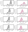 |
Fig. A.1. Distributions of SDSS magnitudes and their corresponding surface brightness. The left panel (grey histograms) show the distribution of ugri magnitudes of SDSS 7934 galaxies from the final sample used in our analysis, while the right panel (dark red hatched histograms) their corresponding surface brightness corrected for the inclination. Median values of all distributions are added in each panel. |
Figure A.2 shows the same plot as Fig. 5 (fitted (u−r) – μu relation for all 14 bins of AFUV) but with an additional background of the whole sample, and also interpolated relations between 22.5 and 27.5 μu.
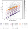 |
Fig. A.2. Relations fitted between observed (u−r) colours and μu for 14 AFUV bins with additional background showing all galaxies used in our analysis. The grey scale colour bar axis shows the value of the AFUV. |
Appendix B: Galaxies with AFUVp< 0
We present here the location in the (u−r)-μu plane galaxies for which the calculated based on Eq. 4AFUVp is lower than zero. Fig. B.1 shows the location of all 426 galaxies with AFUVp< 0.
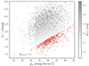 |
Fig. B.1. Fiducial AFUV values from the GSWLC catalogue in the (u−r)-μu plane. Similarly, as in Fig. A.2, grey scale colour bar axis shows the value of the AFUV. Additionally, galaxies with calculated AFUVp< 0 are marked as open orange squares. |
Appendix C: Other colour−surface brightness relatons
Relations fitted between observed colours and surface brightness in different configurations for 14 AFUV bins are presented in Fig. C.1. The sequence of colours represents the one used for AFUV bin in Fig. 4. Filled areas mimic the ±1σ uncertainty around estimated lines. The black line on each panel represents the linear fit to all bins. The slope of this mean relation is shown on each panel.
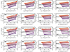 |
Fig. C.1. Exemplary colour – surface brightness-fits for all 14 AFUV bins. Colors are the same as in Fig. 5 and Fig. A.2. The black lines shown in each panel represent the linear slope between colour and surface brightness calculated for the whole sample. |
Appendix D: AFUV bins fitting
Here, we present separate fits performed for all 14 AFUV bins. Each panel represent one bin. At the top of each panel, we give the AFUV range and the number of galaxies from our sample. The fitted linear relation, as well as the deviation of the (u−r) colour from the linear fit (Δur) and the variability of AFUV within the range of ±1σ, are given in each panel.
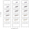 |
Fig. D.1. Relation between observed (u−r) and μu for the sample of 7 934 galaxies divided into 14 AFUV bins. Each panel represents consecutive AFUV bins (Fig. 4 and Table 2). The resulting slope and intercept of the fit are provided within each corresponding panel. The deviation of the (u−r) colour from the linear fit (Δur) and the variability of AFUV within the range of ±1σ from the linear fit (σAFUV) are both indicated in each panel. |
All Tables
All Figures
|
Fig. 1. Main physical properties used in our analysis. Panels above show spectroscopic redshift, stellar mass (log(Mstar/M⊙)), attenuation in the FUV band (AFUV), SFR and specific SFR (sSFR), both in logarithmic scale. The last bottom right panel shows the axis ratio (semi-minor/semi-major) from Meert et al. (2015). Black histograms represent distributions obtained from the whole sample of 29 487 galaxies (0.01 < z < 0.30), while maroon hatched histograms show distributions for the final sample used for the analysis (7986 galaxies). Legends show median values for all parameters calculated for the initial (black histograms) and final (maroon hatched histograms) samples. |
| In the text | |
|
Fig. 2. Attenuation in the FUV band (AFUV) as a function of redshift. Two horizontal lines, dashed and dotted, represent the 1st and the 99th percentile of the AFUV distribution, respectively. The solid vertical line indicates redshift equal to 0.1, while the dashed double-dotted line represents a redshift cut at 0.025. Above that redshift line, the sample cannot probe the most extreme AFUV values. |
| In the text | |
|
Fig. 3. Distribution of log(sSFR/yr−1) for the selected 7 986 galaxies in the redshift range 0.025 < z < 0.1. A vertical solid line and two vertical dotted lines represent the mean value of sSFR of the sample, and the mean value of the sSFR decreased/increased by 4σ of the distribution, respectively. |
| In the text | |
|
Fig. 4. Distribution of AFUV for the final sample of 7814 main sequence galaxies in the redshift range 0.025 − 0.1. The palette of colours represents the AFUV bins used in our analysis. The mean AFUV value for each bin ( |
| In the text | |
|
Fig. 5. Relations fitted between observed (u−r) colours and μu for 14 AFUV bins. The sequence of colours represents the one used for AFUV bin in Fig. 4. Filled areas display the ±1σ uncertainty around estimated lines. |
| In the text | |
|
Fig. 6. Slopes and intercept from (u−r)–μu fits. Interpolated slopes (left axis) and intercepts (right axis) obtained from linear fits for all 14 bins of AFUV (Fig. D.1), as a function of AFUV. The left axis represents slopes (purple full diamonds), and the right axis represents intercepts (red full circles). Linear fits and associated fitted parameters are presented using dashed-dotted lines for slopes and dashed lines for intercepts. |
| In the text | |
|
Fig. 7. Main properties of obtained AFUV priors. Panel a shows the distributions of original AFUV from the Salim et al. (2018) work obtained from careful SED fitting based on measurements from UV to mid-IR (AFUV, blue left hatched histogram), and AFUVp calculated based on Eq. (4) (orange right hatched histogram). Panel b presents the distribution of the difference between AFUV and AFUVp and denotes its median value. In panel c, the difference between AFUV and AFUVp is shown as a function of redshift. We removed for clarity from panel a 426 galaxies, for which calculated AFUVp was lower than 0. |
| In the text | |
|
Fig. 8. Difference between SFR and Mstar from the original GSWLC catalogue (Salim et al. 2018), and those obtained in this work. The difference ΔMstar was calculated as log(Mstar this work/Mstar); and ΔSFR was obtained in an analogous way. Panels a and b show the difference in the stellar masses and SFRs, correspondingly, as a function of redshift, with shaded areas represent standard deviation of the scatter; panels c and d present the relation between the fiducial values and the estimates obtained in this work, with contours showing the distribution of the data. Runs based on GSWLC set of parameters, FULL–run, are shown in blue-coloured lines, while those obtained from LIGHT–run – in an orange-coloured set of lines. Black solid lines visible in panels c and d represent 1:1 relations. |
| In the text | |
|
Fig. 9. Comparison of physical properties obtained in FULL–run, and LIGHT–run runs. Upper panels present results obtained based on FULL–run parameter sets (332 640 templates per redshift bin), while the results shown in bottom panels were estimated based on the LIGHT–run sets of parameters (5544 templates per redshift bin). Black contours shown in each panel correspond to fiducial values from the GSWLC-X2 catalogue (SFR, Mstar), while orange contours illustrate physical parameters estimated in this work. The left column presents results obtained without priors, the middle column – with AFUVs from the GSWLC catalogue, and the right column – with AFUVp calculated from Eq. (4). |
| In the text | |
|
Fig. A.1. Distributions of SDSS magnitudes and their corresponding surface brightness. The left panel (grey histograms) show the distribution of ugri magnitudes of SDSS 7934 galaxies from the final sample used in our analysis, while the right panel (dark red hatched histograms) their corresponding surface brightness corrected for the inclination. Median values of all distributions are added in each panel. |
| In the text | |
|
Fig. A.2. Relations fitted between observed (u−r) colours and μu for 14 AFUV bins with additional background showing all galaxies used in our analysis. The grey scale colour bar axis shows the value of the AFUV. |
| In the text | |
|
Fig. B.1. Fiducial AFUV values from the GSWLC catalogue in the (u−r)-μu plane. Similarly, as in Fig. A.2, grey scale colour bar axis shows the value of the AFUV. Additionally, galaxies with calculated AFUVp< 0 are marked as open orange squares. |
| In the text | |
|
Fig. C.1. Exemplary colour – surface brightness-fits for all 14 AFUV bins. Colors are the same as in Fig. 5 and Fig. A.2. The black lines shown in each panel represent the linear slope between colour and surface brightness calculated for the whole sample. |
| In the text | |
|
Fig. D.1. Relation between observed (u−r) and μu for the sample of 7 934 galaxies divided into 14 AFUV bins. Each panel represents consecutive AFUV bins (Fig. 4 and Table 2). The resulting slope and intercept of the fit are provided within each corresponding panel. The deviation of the (u−r) colour from the linear fit (Δur) and the variability of AFUV within the range of ±1σ from the linear fit (σAFUV) are both indicated in each panel. |
| In the text | |
Current usage metrics show cumulative count of Article Views (full-text article views including HTML views, PDF and ePub downloads, according to the available data) and Abstracts Views on Vision4Press platform.
Data correspond to usage on the plateform after 2015. The current usage metrics is available 48-96 hours after online publication and is updated daily on week days.
Initial download of the metrics may take a while.