| Issue |
A&A
Volume 675, July 2023
|
|
|---|---|---|
| Article Number | A37 | |
| Number of page(s) | 24 | |
| Section | Extragalactic astronomy | |
| DOI | https://doi.org/10.1051/0004-6361/202245290 | |
| Published online | 29 June 2023 | |
Kinematic analysis of the super-extended H I disk of the nearby spiral galaxy M 83⋆,⋆⋆
1
Argelander-Institut für Astronomie, Universität Bonn, Auf dem Hügel 71, 53121 Bonn, Germany
e-mail: eibensteiner@astro.uni-bonn.de
2
Department of Astronomy, The Ohio State University, 4055 McPherson Laboratory, 140 West 18th Ave, Columbus, OH, 43210
USA
3
Center for Astrophysics, Harvard & Smithsonian, 60 Garden St., 02138 Cambridge, MA, USA
4
Dept. of Physics, University of Alberta, Edmonton, Alberta, T6G 2E1
Canada
5
Max Planck Institute for Astronomy, Königstuhl 17, 69117 Heidelberg, Germany
6
Sterrenkundig Observatorium, Universiteit Gent, Krijgslaan 281 S9, 9000 Gent, Belgium
7
Netherlands Institute for Radio Astronomy (ASTRON), Oude Hoogeveensedijk 4, 7991 PD Dwingeloo, The Netherlands
8
Kapteyn Astronomical Institute, University of Groningen, PO Box 800 9700 AV Groningen, The Netherlands
9
Department of Astronomy, University of Cape Town, Private Bag X3, 7701 Rondebosch, South Africa
10
Department of Physics & Astronomy, Bloomberg Center for Physics and Astronomy, Johns Hopkins University, 3400 N. Charles Street, Baltimore, MD, 21218
USA
11
Department of Astronomy, University of Cape Town, Private Bag X3, Rondebosch, 7701
South Africa
12
Department of Physics and Astronomy, West Virginia University, White Hall, Box 6315 Morgantown, WV, 26506
USA
13
Center for Gravitational Waves and Cosmology, West Virginia University, Chestnut Ridge Research Building, Morgantown, WV, 26505
USA
14
National Radio Astronomy Observatory, 1003 Lopezville Road, Socorro, NM, 87801
USA
15
European Southern Observatory, Karl-Schwarzschild Straße 2, 85748 Garching bei München, Germany
16
Observatorio Astronómico Nacional (IGN), C/ Alfonso XII, 3, 28014 Madrid, Spain
17
Univ Lyon, Univ Lyon1, ENS de Lyon, CNRS, Centre de Recherche Astrophysique de Lyon UMR5574, 69230 Saint-Genis-Laval, France
18
National Radio Astronomy Observatory, 520 Edgemont Rd, Charlottesville, VA, 22903
USA
19
Institüt für Theoretische Astrophysik, Zentrum für Astronomie der Universität Heidelberg, Albert-Ueberle-Strasse 2, 69120 Heidelberg, Germany
20
Research School of Astronomy and Astrophysics, Australian National University, Canberra, ACT, 2611
Australia
21
Astrophysics Research Institute, Liverpool John Moores University, 146 Brownlow Hill, Liverpool, L3 5RF
UK
22
Department of Physics & Astronomy, University of Wyoming, Laramie, WY, 82071
USA
23
Cosmic Origins Of Life (COOL) Research DAO, Munich, Germany
24
Departamento de Fisica de la Tierra y Astrofisica & IPARCOS, Facultad de CC Fisicas, Universidad Complutense de Madrid, 28040 Madrid, Spain
25
Astronomisches Rechen-Institut, Zentrum für Astronomie der Universität Heidelberg, Mönchhofstraße 12-14, 69120 Heidelberg, Germany
26
Sub-department of Astrophysics, Department of Physics, University of Oxford, Keble Road, Oxford, OX1 3RH
UK
27
Max-Planck-Institut für Radioastronomie, Radioobservatorium Effelsberg, Max-Planck-Strasse 28, Munich, Germany
Received:
24
October
2022
Accepted:
24
March
2023
We present new H I observations of the nearby massive spiral galaxy M 83 taken with the JVLA at 21″ angular resolution (≈500 pc) of an extended (∼1.5 deg2) ten-point mosaic combined with GBT single-dish data. We study the super-extended H I disk of M 83 (∼50 kpc in radius), in particular disk kinematics, rotation, and the turbulent nature of the atomic interstellar medium. We define distinct regions in the outer disk (rgal> central optical disk), including a ring, a southern area, a southern arm and a northern arm. We examine H I gas surface density, velocity dispersion, and noncircular motions in the outskirts, which we compare to the inner optical disk. We find an increase of velocity dispersion (σv) toward the pronounced H I ring, indicative of more turbulent H I gas. Additionally, we report over a large galactocentric radius range (until rgal ∼ 50 kpc) where σv is slightly larger than thermal component (i.e., > 8 km s−1). We find that a higher star-formation rate (as traced by far UV emission) is not necessarily always associated with a higher H I velocity dispersion, suggesting that radial transport could be a dominant driver for the enhanced velocity dispersion. Furthermore, we find a possible branch that connects the extended H I disk to the dwarf irregular galaxy UGCA 365 and that deviates from the general direction of the northern arm. Lastly, we compare mass flow rate profiles (based on 2D and 3D tilted ring models) and find evidence for outflowing gas at rgal ∼ 2 kpc, inflowing gas at rgal ∼ 5.5 kpc, and outflowing gas at rgal ∼ 14 kpc. We caution that mass flow rates are highly sensitive to the assumed kinematic disk parameters, in particular to inclination.
Key words: ISM: kinematics and dynamics / radio lines: galaxies / galaxies: groups: individual: M 83
A copy of the combined datacube is available at the CDS via anonymous ftp to cdsarc.cds.unistra.fr (130.79.128.5>) or via https://cdsarc.cds.unistra.fr/viz-bin/cat/J/A+A/675/A37
© The Authors 2023
 Open Access article, published by EDP Sciences, under the terms of the Creative Commons Attribution License (https://creativecommons.org/licenses/by/4.0), which permits unrestricted use, distribution, and reproduction in any medium, provided the original work is properly cited.
This article is published in open access under the Subscribe to Open model. Subscribe to A&A to support open access publication.
1. Introduction
The massive, extended atomic gas reservoirs that often surround spiral galaxies usually extend far beyond the inner optical disk (2 − 4 × r25, where r25 is the optical radius; e.g., Wang et al. 2016). These reservoirs may eventually serve as the fuel for star formation in the inner disk and may represent a key component for facilitating accretion from the circumgalactic medium (CGM) and cosmic web (see, e.g., review by Sancisi et al. 2008). However, the details of star formation in outer disks, the origin, the nature of turbulence (traced for example by H I velocity dispersion), and, perhaps most importantly, radial gas flows all remain topics in need of more study.
Observing the extent of neutral atomic hydrogen (H I) gas is important, as it traces the kinematics in disk galaxies, which give further insights into the understanding of galaxy evolution. The 21-cm line emission of H I is often used to examine either disk kinematics and rotation on large scales (e.g., de Blok et al. 2008; Heald et al. 2011; Schmidt et al. 2016; Oman et al. 2019; Di Teodoro & Peek 2021) or the turbulent nature of the interstellar medium (ISM) on small scales (e.g., Tamburro et al. 2009; Ianjamasimanana et al. 2012, 2015; Mogotsi et al. 2016; Koch et al. 2018). In the first case, H I traces the process of gas accreting from the intergalactic medium that flows through diffuse filamentary structures into the CGM of galaxies and further onto the galaxy disk (e.g., Kereš et al. 2005). The gas entering the halo remains cool as it falls onto the disk (i.e., the cold mode scenario in Kereš et al. 2005). This cold accretion dominates in the lower H I density environments (e.g., White & Frenk 1991; Kereš et al. 2005; Tumlinson et al. 2017). In the second case, H I is used to analyze velocity profiles and line widths (i.e., H I velocity dispersion) in order to interpret the thermal states of the optically thin warm neutral medium (WNM; as one of the two phases predicted by models from, e.g., Field et al. 1969; Wolfire et al. 1995, 2003; Bialy & Sternberg 2019). This approach has been found to be valid down to 100 pc scales (e.g., Koch et al. 2021), for example, from emission and absorption studies in the Large and Small Magellanic Cloud (Stanimirovic et al. 1999; Jameson et al. 2019).
The exact amount of H I gas in the outskirts of nearby galaxies was analyzed in Pingel et al. (2018) and Sardone et al. (2021). Pingel et al. (2018) analyzed and compared four galaxies out of 24 total sources of the Hydrogen Accretion in LOcal GAlaxies Survey (HaloGAS; see Heald et al. 2011 for the survey paper) made with Green Bank Telescope (GBT) observations. The authors found that the H I mass fraction below H I column densities of NHI = 1019 cm−2 (i.e., diffuse H I gas) is on average 2%. Furthermore, their GBT observations of NGC 925 revealed a detection of ∼20% more H I than observations done with the Very Large Array (VLA) as part of The H I Nearby Galaxy Survey (THINGS; Walter et al. 2008). This finding underscores, among other aspects, that the THINGS VLA interferometric observations require a correction for missing short-spacing observations. Sardone et al. (2021) studied 18 out of a total of 30 nearby disk and dwarf galaxies of the MeerKAT H I Observations of Nearby Galactic Objects: Observing Southern Emitters (MHONGOOSE; see de Blok et al. 2016 for the survey paper) and found that 16 out of the 18 observed galaxies have 0.02 to three times additional H I mass outside of their optically bright disks.
The nearby (D = 5.16 Mpc) grand-design spiral galaxy M 83 (also known as NGC 5236; see Table 1) is massive, favorably oriented (i = 48°), and associated with active star formation (see Table 1), which has made it a classic target of several studies of the H I in outer portions of disk galaxies (e.g., Huchtmeier & Bohnenstengel 1981; Tilanus & Allen 1993; Miller et al. 2009). Moreover, M 83 was one of the first galaxies where the tilted ring analysis was performed (Rogstad et al. 1974, see their Fig. 8). Sensitive, wide-area H I imaging of M 83 has revealed its highly extended, structured disk as well as a northern spiral arm-like structure (e.g., Heald et al. 2016; Koribalski et al. 2018). However, previous high-resolution interferometric observations (see e.g., Walter et al. 2008; Bigiel et al. 2010a) have been restricted to single central pointing with the VLA (0.5° primary beam). In this paper, we present a ten-field mosaic using the VLA with an angular resolution of 21″ (∼500 pc) corrected for short-spacing using GBT observations (see Sect. 2.3).
Properties of M 83, NGC 5236.
The aim of this paper is to study the large- and small-scale kinematics of the H I in M 83’s outskirts (rgal > r25). To this end, we look at individually defined regions and compare their H I properties to the central (optical) disk. We search for deviations from pure circular motions and asymmetries in the outskirts. We examine radial trends in velocity dispersion and environmental differences between the defined regions. We also highlight the effects of different kinematic parameters (based on 2D and 3D tilted ring models) on average radial mass flow rates and tilted ring modeling in general.
The paper is structured as follows: In Sect. 2 we describe how the VLA observations were taken, calibrated, and imaged along with how we convert observational measurements into physical quantities. In Sect. 3, we present the distribution of H I across M 83, its velocity field, and environmental differences of H I (H I gas surface density, ΣHI) and kinematic parameters (H I velocity dispersion, line-of-sight velocities, and residual velocities). In Sect. 4, we discuss the environmental dependence of the observed H I velocity dispersion along with the northern extended arm of M 83 and M 83’s possible interaction with a nearby dwarf irregular galaxy UGCA 365. In Sect. 5, we show upper limits for average radial mass flow rates (based on 2D and 3D tilted ring models), discuss the limitations, and compare the mass flow rates to those from the literature.
2. Observations, data reduction, and products
2.1. Observations
The observations of M 83 were carried out with the VLA. We obtained a ten-point mosaic using the dual-polarization L-band of the VLA to map the 21-cm emission of neutral hydrogen over the entire super-extended disk of the nearby galaxy M 83 (see Figs. 1 and 2). Most of the data were taken February 2014 through January 2015 for approximately 40 hours over the course of 22 runs (project codes: 13B-196, 14B-192, PI: F. Bigiel). We used the VLA in three hybrid configurations, D north C (DnC), C north B (CnB), and B north A (BnA), to ensure good u–v coverage despite M83’s southern declination. We chose a time split for the configurations similar to THINGS’ observing strategy (see Table 2). We chose a velocity resolution of 0.5 km s−1 and a bandwidth of 4 MHz corresponding to 860 km s−1, which is well suited to resolve the H I line and cover the full range of 21-cm emission from the galaxy with enough bandwidth for continuum subtraction. At the beginning of each observing session, we observed the bandpass calibrator 3C286 for approximately ten minutes. Observations were then set up so that two of the ten mosaic pointings were observed in succession for ten minutes each. The sessions were followed by observations of the gain calibrator (J1331-2215). During each session, the gain calibrator was observed six times. We show a summary of our observations in Table 2.
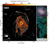 |
Fig. 1. Integrated intensity map (moment 0) for H I emission across the disk of M 83 at a resolution of 21″. The black circle in the lower left corner marks the beam size of 21″ (≈500 pc). The black to white colorbar indicates integrated intensities from 0 − 100 K km s1 and the orange to yellow integrated intensities above 101 K km s1. We denote the companion galaxy UGCA 365 which in projection is ∼55 kpc away from the center of M 83. To the right, we show the enclosed optical disk (r25 ∼ 8 kpc) overlaid with H I column density contour (NHI = 13 × 1019 cm−2) extending over a radius of ∼40 kpc. For visualization reasons, we show unfilled NHI contours for the high resolution optical image. Beyond 10 kpc we show filled NHI contours. The white line surrounding M 83 shows the field of view (FoV; i.e. the full mosaic coverage) of the VLA observation. (optical image credits: CTIO/NOIRLab/DOE/NSF/AURA, M. Soraisam; Image processing: Travis Rector, Mahdi Zamani & Davide de Martin; low resolution background > 10 kpc: DSS2). |
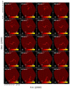 |
Fig. 2. Channel maps of our VLA+GBT data. The line-of-sight velocity of the shown channels is displayed on the upper left corner of each panel and the colorbar is shown in units of K. For visual purpose we only show every third 5.0 km s−1 channel (i.e. we do not integrate over channels). The companion galaxy UGCA 365 is detected in the velocity channels 559 km s−1 and 574 km s−1. We show all channels in the appendix (see Appendix B). |
Summary of our VLA H I observation across M 83.
2.2. Reduction
The VLA pipeline implemented in CASA (McMullin et al. 2007; version: 5.4.2-8.el6) was used without Hanning smoothing, as recommended by the VLA pipeline guide1, for each of the science blocks. The flagging summary showed us that one to a maximum of two antennas were completely flagged for some science blocks. As a next step, we reduced the data to include only the spectral window (spw) where the H I emission is located (rest-frequency ∼1.420 GHz) using the CASA task split. This was followed by producing various diagnostic plots with a focus on the calibrator sources and applying additional data flagging (e.g., spikes of radio frequency interference or baselines) by hand using the CASA task flagdata.
We then ran a standard calibration script where we calibrated the flux, bandpass, and gain using gaincal. As the calibrators did not show any discrepancies, we merged all science blocks via the CASA function concat. This resulted in a measurement set containing only the H I spw with the target field scans (ten pointing). During our first run of a test tclean, we noticed horizontal and vertical stripes in the channels around the local standard of rest velocity of 380 km s−1. We carried out several additional rounds of manual flagging to identify and remove corrupted baselines. We inspected amplitudes and phases for the data from all baselines by eye, finding some corrupt baselines that we flagged.
2.3. Imaging
To create “images” of our VLA observation, we used the CASA task tclean, which combines multiple arrays, and deconvolved using the multiscale clean algorithm (Cornwell 2008). We used the mosaic gridding algorithm and weighed the u − v data according to the Briggs scheme with a robustness parameter r = 0.5, which balances spatial resolution and surface brightness sensitivity. We tried several settings (for example, (i) restoringbeam = 15″ with cell = 5″ and (ii) restoringbeam = 21″ with cell = 7″) and found that a resolution of 21″ (restoringbeam = 21.0) and a spectral resolution of 5 km s−1 (see Table 3) provides a good compromise between resolution and noise. Since our observations have more integration time and substantially better surface brightness sensitivity in the D-configuration data, our choice of weighting naturally produced a synthesized beam size that is comparable to the D-configuration beam (46″; see Table 3). We restricted the deconvolution by using a clean mask derived from CASA’s automasking scheme (Kepley et al. 2020) with the following sub-parameters: sidelobethreshold = 0.75, noisethreshold = 3.0, lownoisethreshold = 2.0, negativethreshold = 0.0, minbeamfrac = 0.1, growiterations = 75. In order to increase the S/N to be sensitive to emission even where the line is faint, we averaged several channels, resulting in a spectral resolution of Δv = 5.0 km s−1. The typical rms per channel observed is ≈3 mJy beam−1.
Properties of our imaged and feathered dataset.
The H I in M 83 is extended compared to the primary beam of the VLA. As a result, subsequent to deconvolution, the interferometric VLA data needed to be combined with single-dish data to correct for the insensitivity of the interferometer to the extended emission. We used the GBT single-dish data obtained as part of the GBT-THINGS project (project GBT11A-055; see for example the maps in Pisano 2014). The GBT data were taken on 6, 12, and 26 March 2011. Either 3C147 or 3C295 was observed as a primary flux calibrator before mapping four square degrees around M 83. We derived a Tcal value of 1.55 K in both polarizations that we used for all observations. We used the GBT spectrometer with a 50 MHz bandwidth for observing in a frequency-switching mode with a 10 MHz throw while making a basket-weave map in RA and Dec. While data were taken with frequency-switching, we used the edge four integrations as an “off” position to calibrate the maps. These correspond to 6.7 arcmin on each edge. Since the extent of M 83 is less than two degrees and the map shows no subtracted H I emission, we find that these are clean “off” positions. A second order polynomial was fit to the spectra over an emission-free region to remove residual baseline structure. Data were boxcar smoothed to 5.15 km s−1 resolution before being imaged with (AIPS). A fourth order polynomial was removed from the final cube the SDGRD task in the Astronomical Image Processing System.
We combined the GBT map with the mosaic interferometer data using the CASA task feather. Some of the emission is very extended and had to be recovered by feathering, so the pixel statistics often reflect this extended emission. Before performing this task, we used the uvcombine python package (Koch & Ginsburg 2022) to find the correct single-dish scaling factor (sdfactor). We used an sdfactor of 1.0 (see Fig. A.1). We regarded lines of sight separated by more than a VLA synthesized beam as being statistically independent. However, because of the feathering process, the noise in the GBT data may have led to weak but spurious correlations up to scales approaching the GBT beam of 523″. Since the surface brightness of the noise in the GBT map is small compared to the VLA data and our results do not depend heavily on the statistical independence of the VLA data, we note this as a caution and proceed. We show properties of the feathered data in Table 3. In Fig. 3, we show the spectra of the VLA and the feathered VLA (VLA plus GBT) cubes after we converted them into units of Kelvin. We found a total flux for the VLA cube of 5.2 × 10⁴ K and 6.6 × 10⁴ K for the feathered one (VLA plus GBT). This difference emphasizes that single-dish data are needed even for interferometric observations, including compact configurations. For comparison we also show in Fig. 3 the spectra over the same field of view from The Local Volume H I Survey (LVHIS; Koribalski et al. 2018 with the Australia Telescope Compact Array – ATCA at ∼113″ ≈ 2.62 kpc scales) and KAT7 observations (seven-dish MeerKAT precursor array; Heald et al. 2016 at ∼230″ ≈ 5.33 kpc scales), which were sampled on the same spectral axis grid. We observed that the KAT7 agrees well with the VLA plus GBT spectra, while LHVIS only agrees on the receding side (i.e., > 510 km s−1). The spectra of VLA plus GBT highlights a significant fraction of emission that we see with the addition of the GBT observation.
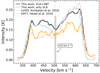 |
Fig. 3. Global H I profile of M 83 from our VLA observations (orange) and the results of feathering the VLA with the GBT observations (black). The systemic velocity appropriate for the centre of the galaxy is indicated with the vertical grey dashed line at 510 km s−1 (see also Table 1). We also show H I observations of the same FoV of M 83 from LVHIS (Koribalski et al. 2018) and KAT7 (Heald et al. 2016) that we have sampled on the same spectral axis grid at their native angular resolution. |
2.4. Data products
After feathering, the data were resampled onto a hexagonal grid with a grid size matching the beam size. This ensured that the resampled measurements are mostly independent. This resulted in 50 574 sightlines separated by a beam size. To improve the S/N, we applied a masking routine based on the methodology introduced by Rosolowsky & Leroy (2006). To this end, we first identified pixels with a high S/N (S/N ≥ 4) and a low S/N (S/N ≥ 2). As a next step, the identified high S/N regions were iteratively grown to include adjacent, moderate S/N regions as defined by the low S/N mask. In this way, we recovered the more extended two-sigma detection that belongs to a four-sigma core. Only pixels detected with an S/N ≥ 3 (where the signal represents the integrated intensity; see next paragraph) were used in subsequent analysis. In this work, we made use of the data products described in the following paragraphs.
The integrated intensity map was created from the masked data cube by integrating along the velocity axis for each of the individual sightlines v multiplied by the channel width Δvchan of 5 km s−1:
![$$ \begin{aligned} I_{\rm HI} \, [\mathrm{K \, km \, s}^{-1}] = \sum _{n_{\rm chan}} I_{ v} \, [\mathrm{K}] \, \Delta { v}_{\rm chan} \, [\mathrm{km \, s}^{-1}]. \end{aligned} $$](/articles/aa/full_html/2023/07/aa45290-22/aa45290-22-eq1.gif)
The uncertainty was calculated by taking the square root of the number of the included channels along a line of sight multiplied by the 1σ root mean squared value of the noise and the channel width:  . We calculated σrms over the signal-free part of the spectrum using the astropy (Astropy Collaboration 2013, 2018) function mad_std that calculates the median absolute deviation and scales it by a factor of 1.4826. This factor results from the assumption that the noise follows a Gaussian distribution. For further analysis2 we focused only on significant detections of S/N = IHI/σHI > 3, resulting in 5539 sightlines separated by a beam size.
We converted the H I 21-cm intensity (IHI) to the H I gas surface density, ΣHI, via:
![$$ \begin{aligned} \Sigma _{\rm HI}~[M_{\odot }~\mathrm{pc} ^{-2}] = 0.015~I_{\mathrm{HI} }~ [\mathrm{K~km~s} ^{-1}] ~ \cos {(i)}. \end{aligned} $$](/articles/aa/full_html/2023/07/aa45290-22/aa45290-22-eq3.gif)
This conversion was used by Bigiel et al. (2010b, among many others), and results in a hydrogen mass surface density and neglects heavy elements. The cos(i) factor corrects for inclination (see Table 1). We derived the H I column density via:
![$$ \begin{aligned} N_{\mathrm{H}\,i }~[\mathrm {cm}^{-2} ] = 1.82\times 10^{18}~ I_{\mathrm{HI} }~[\mathrm{K~km~s} ^{-1}]. \end{aligned} $$](/articles/aa/full_html/2023/07/aa45290-22/aa45290-22-eq4.gif)
Our aim with the use of velocity fields was to obtain an accurate characterization of the dynamics in a galaxy. For this purpose, each pixel was assigned a velocity that represents the average line-of-sight velocity of the gas. However, this is not trivial, and multiple approaches have been used in the literature that differ from one another, each with some advantages and disadvantages (see de Blok et al. 2008 for a discussion on peak velocity fields, Gaussian profiles, multiple Gaussian profiles, and Hermite h3 polynomials methods). In this work, the first moment we took for the observed velocity field can be expressed as follows:
![$$ \begin{aligned} V_{\rm los} [\mathrm{km \, s}^{-1}] = \frac{\sum {I_{\nu }} [\mathrm{K}] \, { v}~[\mathrm{km \, s}^{-1}]~\Delta { v}_{\rm chan} [\mathrm{km \, s}^{-1}]}{{I}_{\rm HI} [\mathrm{K~km~s}^{-1}]}. \end{aligned} $$](/articles/aa/full_html/2023/07/aa45290-22/aa45290-22-eq5.gif)
We used the width of the H I emission line to trace the velocity dispersion (σv) along each line of sight. Several methods exist to estimate the width of an emission line: fitting the line profiles with a simple Gaussian function or Hermite polynomials or calculating the second moment. In this work, we calculated the velocity dispersion σv following the (i) effective width, σeff, approach used in, for example, Heyer et al. (2001), Leroy et al. (2016), and Sun et al. (2018):
![$$ \begin{aligned} \sigma _{\mathrm{eff} }~[\mathrm{km~s} ^{-1}]= \frac{\textit{I}_{\mathrm{HI} }~[\mathrm{K~km~s} ^{-1}]}{T_{\rm peak}~\mathrm{[K]} ~\sqrt{2 \pi }}. \end{aligned} $$](/articles/aa/full_html/2023/07/aa45290-22/aa45290-22-eq6.gif)
We divided the velocity-integrated intensity by the peak brightness temperature, Tpeak. We then converted this value to the standard intensity-weighted velocity dispersion by dividing it by  – the conversion constant for a Gaussian profile. This definition of σ has the advantage that it is less sensitive to noise, but it will mis-characterize line profiles that significantly deviate from a single Gaussian.
We did not subtract the finite channel width (i.e., line broadening caused by the instrument) as it is done, for example, for extragalactic CO observations (e.g., Sun et al. 2018). The usual finite correction factor will overcorrect given that 5 km s−1 ≈ the WNM thermal width.
We also calculated σv with (ii) the square root of the second moment:
![$$ \begin{aligned} \begin{aligned} \sigma _{\sqrt{\mathrm{mom2} }}~[\mathrm{km~s} ^{-1}] = \left\{ \frac{\sum I_{\nu }\mathrm ~[K]~(v~[km \, s^{-1}] -V_{\rm los}~[\mathrm{km \, s}^{-1}])^{2}}{\sum I_{\nu }~\mathrm{[K]} }\right\} ^{1/2} . \end{aligned} \end{aligned} $$](/articles/aa/full_html/2023/07/aa45290-22/aa45290-22-eq8.gif)
We compare (i) σeff and (ii)  in Sect. 4.1.
2.5. Radial profiles – Binning and stacking
Throughout this work, we make use of radial profiles, binning in galactocentric rings of 1 kpc width (roughly twice the beam size of 500 pc). Each point in these profiles thus represents the average within a given ring defined by the structure parameters (Table 1).
In order to average (“stack”) spectra within a given ring, we aligned the spectra to the peak velocity (see e.g., Jiménez-Donaire et al. 2019; Bešlić et al. 2021; or for H I related science Koch et al. 2018, who discussed different stacking approaches, i.e., different definitions of the line center Vrot, Vcent, and Vpeak). We created stacks again in ∼1 kpc-wide galactocentric rings.
2.6. Tilted ring kinematics
H I rotation curves are most commonly derived from velocity fields. The quantity that is accessible through observations is the line-of-sight velocity (Vlos). To infer the rotational velocities of the gas in the disk from measurements of Vlos, we had to utilize a specific model that could be fitted to the data.
The “tilted ring” approach describes a galaxy by a set of rings, each of which has their own inclination i, position angle, systemic velocity Vsys, center position (x0, y0), and rotation velocity Vrot. Under the assumption that the gas moves in circular orbits within each ring, we could then describe Vlos, obs for any position (x, y) on a ring with radius r as:
The inclination i of the disk together with the azimuthal angle θ and the radius r form a polar coordinate frame.
2.6.1. Adopted tilted ring model for M 83
Several kinematic parameters for M 83 exist in the literature. However, the rotation curve that extends the farthest and is readily available was published in Heald et al. (2016) and uses KAT7 (the seven-dish MeerKAT precursor array) observations with an angular resolution of ∼230″≈5.33 kpc. Since H I in M 83 extends far in our observations, this is the best suited rotation curve that involves the northern and southern arms of M 83 (see Sect. 3.1). In addition, Heald et al. (2016) performed several tilted ring models explicitly for this galaxy, which strengthens our selection of this rotation curve over others. They used the Groningen Image Processing System (GIPSY) task rotcur to construct a rotation curve (Vrot) using a ring width of 100″. For that, they set the radial velocity component (Vrad) to zero, which reduces Eq. (7) to the first two terms. Heald et al. (2016) found at radii beyond 1000″ ∼ 23 kpc, an opposite deviation of the modeled approaching and receding rotation curves. To account for this, they used Vsys = 510 km s−1 for r < 23 kpc and Vsys = 500 km s−1 for r > 23 kpc. In this work, we adopt their resulting kinematic parameters from this approach (see also discussion in Sect. 5.1).
To get a modeled velocity map (Vlos, mdl), we used their rotation curve (Vrot(r)), their constant inclination angle of 48°, and, their position angles, which vary from 225.0° for the central ring to 158.6° for the outermost ring:

Here, Vsys is the systemic velocity of the galaxy with respect to the observer, and Vrot is the rotation velocity. The Vlos, mdl is denoted in sky coordinates (x, y), while the terms on the right side of Eq. (8) are in the disk coordinate frame (r, θ). These two systems are related:
and sin(θ) from Eq. (7) as:
where x0 and y0 denote the center coordinates and the position angle is the angle measured counter-clockwise between the north direction of the sky and the major axis of the receding half of the galaxy. We then used Eq. (8) to get Vlos, mdl. For the purpose of showing Vlos, mdl maps (and Vres maps, see next paragraph), we interpolated the space between the rings (see Fig. 11) and applied a simple mask to only show Vlos, mdl values that match with our observed S/N masked velocity field (i.e., we ignored data outside the mask).
2.6.2. Residual velocities and radial velocities
To determine the residual velocities (Vres), we subtracted Eq. (8) from Eq. (7), Vres(x, y) = Vlos, obs(x, y)−Vlos, mdl(x, y) and obtained:

To get radial velocities (Vrad), we only took Vres values within each tilted ring (i.e., we did not use the Vres map where we interpolated between the gaps) and accounted for the sin(θ)sin(i) term:
Knowing in which direction a galaxy rotates is required to correctly interpret the nature of measured radial motions. Negative (positive) velocities in Vrad are inflow (outflow) motions when a galaxy is rotating clockwise, and they are outflow (inflow) motions when a galaxy is rotating counterclockwise. Under the assumption that spiral galaxies spin with their arms trailing in the direction of rotation, the winding of the extended H I arms reveal that M 83 rotates clockwise. Therefore, Vrad < 0 indicates inflow and Vrad > 0 indicates outflow for M 83.
3. Results
In this section, we present the results derived from our H I observations toward M 83 (integrated intensity map and velocity fields, Figs. 1 and 4) and analyze how the super-extended H I disk of M 83 compares to its optical central disk. To do this, we applied a simple environmental mask by visually separating these regions (see Fig. 5), as it allowed us to distinguish between (i) the central disk, (ii) ring, (iii) southern area, (vi) southern arm, and (v) northern arm.
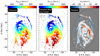 |
Fig. 4. Observed, adopted, and residual velocity maps. Observed: velocity field of M 83 using our VLA H I observations. The blue colors represent the approaching and the red is the receding side of the H I galaxy disk. Adopted tilted ring model: constructed velocity field using Vsys, Vrot, i, and position angle of the tilted ring model by Heald et al. (2016). The green colors represent the systemic velocity of ∼510 km s−1 for the inner ∼23 kpc in galactocentric radius and ∼500 km s−1 beyond (see Sect. 2.6.1). The tilting results in gaps between the rings, which we interpolated for the presentation of these maps (2d interpolation, see Fig. 11). We had to restrict our field of view to the model outputs (i.e. the outermost tilted ring). Residual: The difference between the observed velocities and the modeled velocities; in the range of −40 to 40 km s−1. |
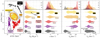 |
Fig. 5. Environmental differences in velocities, H I gas surface density and velocity dispersion in M 83. Mask: colors represent the different regions: central disk, ring, southern area, northern arm and the southern arm. We note the total sightlines for each of the regions. The grey colors in the background show the H I column density contours (NHI = 13 × 1019 cm−2) that we showed in Fig. 1. Violin plots: each violin represents the distribution of each quantity in a region defined in the mask. We set the kernel density estimation (KDE) to compute an empirical distribution of each quantity to 200 points. The columns on the x axis show the H I gas surface density ΣHI, the second the line width σeff, the observed velocities Vlos, and the last residual velocities Vres. The mean value of the observed quantity is reported for each violin. The long tails seen for example in the Vlos violin for the northern arm represents that there is one discrepant value. |
3.1. Distribution of H I in M 83
In Fig. 1 we show the integrated H I intensity map of M 83 that extends over one degree in the sky. The H I emission toward the central optical disk is ∼8.1 kpc in radius and shows the highest integrated intensities. The right panel in Fig. 1 shows an optical image of M 83’s central disk with H I column densities in cyan contours. These contours extend up to a radius of 50 kpc (approximately four times the size of the optical disk).
The central disk is surrounded by H I emission that follows a ring-like structure that extends to a galactocentric radius of ∼16 kpc. The most prominent features in the outskirts of M 83 are the southern and northern spiral-like structures seen already in previous studies (e.g., Bigiel et al. 2010a; Heald et al. 2016). Our field of view (gray solid line in Fig. 1) allowed us to also detect the nearby companion galaxy cataloged as UGCA 365, which is 5.25 ± 0.43 Mpc in distance (the red giant branch – TRGB – measurements; Karachentsev et al. 2007). We measured that this dwarf irregular galaxy is ∼50 kpc in projected distance from the center of M 83 and has in our map a diameter of 88″ (≈2 kpc). This is a factor of two smaller than what has been found by Heald et al. (2016). We found an H I mass of MHI = 6.1 × 10⁵ M⊙, which differs from the quoted H I mass in Heald et al. 2016, who find MHI = 2.7 × 10⁷ M⊙. We attribute this difference to the fact that our VLA observations are not as sensitive as the KAT-7 data. This companion galaxy was faintly detected in the GBT observations (see Fig. C.1).
Throughout this work, we refer to different regions: the central disk, where we found an averaged H I column density of 6.28 × 1020 cm−2; the ring that surrounds the central disk; and the prominent northern arm and southern arm. In the southwest, we detected significant emission with spots of enhanced column densities; we refer to this region as the southern area.
3.2. Velocity fields
In this work, we analyze observed and modeled first-moment maps to examine noncircular motions. The observed velocities, Vlos, obs, in the first panel of Fig. 4 range from 357 to 661 km s−1, where 510 km s−1 is the systemic velocity (shown as green colors, see also Table 1) for the inner ∼23 kpc in the galactocentric radius and ∼500 km s−1 beyond (see Sect. 2.6.1). The central disk shows symmetric velocity behaviors that are typical for gas moving in circular motions. However, this symmetry breaks at larger radii. The ring already presents differences in the systemic velocity and the corresponding approaching and receding velocities, as the symmetry axis is no longer the major and minor axis of the central disk. The northern arm only shows approaching velocities, whereas the southern arm shows a transition from systemic to receding velocities along the arm direction. Both of the arms are winding clockwise, similar to the spiral arms seen in the central (optical) disk from, for example, CO observations (e.g., Koda et al. 2020).
The second panel of Fig. 4 shows the line-of-sight velocity field implied by the Heald et al. (2016) tilted ring model (we used their Vrot, i, and position angle for each tilted ring; we describe the procedure and our motivation to use this set of kinematic parameters in Eq. (8) and Sect. 2.6.1). The field of view was restricted to the model outputs, meaning that we neglected everything beyond the outermost tilted ring (including the northern companion galaxy UGCA 365). In this map, we observed lower approaching velocities toward the beginning of the northern arm and higher receding velocities in the southern area compared to the observed velocities.
The third panel in Fig. 4 shows the residual velocities, Vres. The highest Vres values are indicated with dark red or dark blue colors in the third panel in Fig. 4. We found values of ∼40 km s−1 in the southwest of the ring along with ∼ − 10 km s−1 on the eastern side. The southern area and southern arm are shown in white to light-blue colors indicating a Vres of ∼0 − 10 km s−1. The northern arm shows negative and positive Vres values, whereas the kink of the arm (inflection point; see Sect. 4.2) has Vres ∼0 km s−1. Additionally, we found at the end of the northern arm a “blob” of negative Vres values of ∼ − 30 km s−1.
3.3. Environmental differences in velocities, H I gas surface density, and velocity dispersion
We analyzed different environmental regions in more detail, as shown in Fig. 5. We did this by masking each individual area by eye based on the emission seen in Fig. 1 after applying an S/N cut (S/N = 3)3. This resulted in the following total number of sightlines separated by a beam size for each region: for the central disk = 678, ring = 1147, southern area = 1174, southern arm = 681, and northern arm = 535. In the following paragraphs, we examine the environmental dependence of ΣHI, σ, Vlos, and Vres in M 83 shown in Fig. 5.
The second column of Fig. 5 shows the H I surface density. Overall, this quantity decreases with galactocentric radius from the central disk to the outermost outskirt region – the northern arm. We found the highest mean ΣHI in the central disk: 5.2 M⊙ pc−2. The ring, southern area, and southern arm showed a mean ΣHI of 3.2 M⊙ pc−2, 2.0 M⊙ pc−2, and 1.8 M⊙ pc−2, respectively. The northern arm exhibited a mean ΣHI of 1.5 M⊙ pc−2, which is more than a factor of approximately three lower than the central disk. The overall trend of decreasing ΣHI with rgal in M 83 agrees with previous studies (e.g., Bigiel et al. 2010a).
The third column of Fig. 5 shows to the first order that the means of the velocity dispersion (using σeff, the effective width; see Eq. (5)) decrease with rgal. Upon closer examination, it became clear that the northern arm has a slightly higher mean line width than the southern arm. However, the overall distributions of these two regions appear reasonably similar. Higher values in σeff could be attributed to multiple components and/or wider components. This way of measuring the velocity dispersion does not distinguish between these possibilities (see discussion in Sect. 4.1). The overall trend of decreasing σ with rgal agrees with previous studies (e.g., Tamburro et al. 2009 and see our discussion in Sect. 4.1).
The last two columns of Fig. 5 show the line of sight and the residual velocities (i.e., Vlos and Vres). In general, the central disk is well described by the tilted ring model (that assumes circular motions), as the distribution of Vlos looks very symmetric and the mean of Vres is close to zero (⟨Vlos⟩ = 0.02 km s−1). The mean value of 510 km s−1 is the same as what was used for systemic velocity in the tilted ring model (until a radius of ∼23 kpc; see Sect. 2.6.1). The ring region is still relatively well characterized by this model, with deviations from pure circular motions of ⟨Vres⟩ = 2.0 km s−1. Also, the southern arm has low mean deviations of ⟨Vres⟩ = −1.9 km s−1; however, the mean Vlos values are on the receding side (i.e., > 510 km s−1, gray dashed horizontal line). The outermost regions, the southern and northern arms, show significant deviations from circular motions. They exhibit ⟨Vres⟩ values of −13.9 km s−1 and −11.8 km s−1, but their means in Vlos are on the receding and approaching side, respectively. The distribution of Vres values toward the northern arm represents a change in velocities along the arm (we discuss this in Sect. 4.2).
We show for each quantity the mean as well as the 16th and 84th percentiles in Table 4. This table already contains values of the IHI-far ultraviolet (FUV) ratio for each region. We discuss a visual comparison of FUV emission (as a tracer of the star-formation rate) and velocity dispersion later in the paper (see Sect. 4.1). Table 4 reveals that the central disk has the smallest IHI/FUV values (i.e., 7.32 × 10⁵ K km s−1/(mJy arcsec−2)). The ring shows the largest values, and IHI/FUV then decreases with rgal.
Properties of environmental regions in M 83.
4. Discussion
In this section, we study the radial dependence of the velocity dispersion (obtained with three different methods) and H I surface density and how it changes beyond the central disk. We further examine possible reasons for broader H I profiles and discuss the extended H I structure of M 83 and its companion UGCA 365.
4.1. H I velocity dispersion in the outskirts of M 83
Multiple observations have shown that the H I velocity dispersion encodes information on a combination of temperature, turbulence, and unresolved bulk motions and is thus sensitive to feedback and energetics and the physical state of the gas (e.g., Tamburro et al. 2009; Ianjamasimanana et al. 2015; Mogotsi et al. 2016; Romeo & Mogotsi 2017; Koch et al. 2018; Oh et al. 2022). In the upper panel of Fig. 6, we show the radial profile of the velocity dispersion across the whole disk of M 83. Overall the velocity dispersion decreases with galactocentric radius, similar to the trend we found in Fig. 5. This agrees also with studies where it was shown that σv decreases with rgal across local disk galaxies (e.g., Tamburro et al. 2009). However, in our radial profile, a peak of velocity dispersion is evident in the region of the ring, which we marked with two vertical dashed lines.
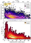 |
Fig. 6. Radial profile of the velocity dispersion, σv, and the H I gas surface density ΣHI, together with the point density of σv and ΣHI for individual lines of sight (circular points; the color-coding reflects a linear density distribution, where the highest density is shown in yellow). Top panel: We compare here the effective width (σeff purple-to-yellow scatter points) and |


In Fig. 6, we make a comparison between three radial profiles obtained with different methods that are commonly used in the literature. We first compare the effective-width approach (σeff colorized markers; see Eq. (5)) with the square root of the second moment ( , gray markers; see Eq. (6)) and show their corresponding profile (gray and pink solid lines). Though σeff is used to study cooling and the physics of the ISM, for studies dealing with dynamics and large-scale evolution, using
  is more appropriate. We additionally show the velocity dispersion profile where we stacked the σeff values (pink-whited dashed line; see Sect. 2.5 for a description of the binning and stacking techniques). We found that the profiles for
  , σeff, and stacking σeff all show, in addition to the center, enhanced velocity dispersion in the ring. The same behavior arose in the ΣHI radial profile shown in the bottom panel of Fig. 6.
From Fig. 6, it is immediately apparent that the profile of  has a higher velocity dispersion than that of σeff. However, the stacked profile shows an alternative behavior: being greater than the median values until r ∼ 40 kpc and then approaching the lower values of the median. Overall, the different approaches show similar trends but are offset by ∼3 km s−1 between σeff and
  and 2 km s−1 between σeff and stacked σeff (taking the mean between the differences until rgal = 40 kpc). Koch et al. (2018) analyzed the differences between these methods in more detail, and they demonstrate that the deviation in
  from the stacked profiles is a strong indication for multiple velocity components in some lines of sight. An analysis toward M 31 and M 33 (Koch et al. 2021) finds more than 50% of the lines of sight have more than one Gaussian in a spectrum, suggesting that multi-Gaussian profiles can be a source of discrepancy. This has also been found in various other nearby galaxy surveys (Warren et al. 2012; Stilp et al. 2013a,b). An examination of the masked ring region reveals some of these features (see Appendix B). A by-eye estimate suggests that more than one-third of the over 1000 lines of sight in the ring have more than one component. A more sophisticated fitting of individual spectra is beyond the scope of this paper and is limited by our need to increase the S/N via smoothing of the data to 5 km s−1 channels (see Sect. 2.3). Nevertheless, σeff and
  show an enhancement in velocity dispersion in the ring.
Line widths of ∼6 − 10 km s−1 have been observed in the outskirts of galaxies (e.g., Tamburro et al. 2009 using the second-moment approach). At pressures that are typical for disk galaxies, the interstellar atomic gas has two phases at which it can remain in stable thermal equilibrium (e.g., Field et al. 1969; Wolfire et al. 1995, 2003). These two phases correspond to the cold neutral medium (CNM) and the WNM with temperatures of ∼100 K and ∼8000 K, respectively. The cold neutral gas emits lines with a characteristic line width of ∼1 km s−1, while the warm neutral gas has a line width of ∼8 km s−1. Tamburro et al. (2009) found spectral lines broader than ∼8 km s−1 in the THINGS galaxies and interpreted them to have been broadened by turbulent motions. However, as mentioned in the previous paragraph, the second-moment approach has been found to overestimate line widths (e.g., Mogotsi et al. 2016; Koch et al. 2018).
The bulk of the gas in the outskirts of galaxies is expected to be in the form of WNM (see e.g., Dickey et al. 2009, who find a CNM fraction of ∼15–20% out of r ∼ 25 kpc in the Milky Way). The WNM temperature does not drop below ∼5000 K (corresponding to σ ∼ 6 km s−1) and is typically closer to 6000 − 7000 K (see e.g., Wolfire et al. 2003). Accordingly, the WNM is not expected to have a thermal velocity dispersion larger than 8 km s−1. We found that the velocity dispersion is higher than the thermal WNM line width (i.e., greater than 8 km s−1; marked as the horizontal dashed line in Fig. 6) for both  and σeff. This agrees with past studies (e.g., Tamburro et al. 2009; Koch et al. 2018; Utomo et al. 2019). Our observations, however, highlight the large galactocentric radius range where we found a shallow decrease in velocity dispersion that is slightly larger than thermal equilibrium – until rgal ∼ 50 kpc. The exact values of the velocity dispersion shown in Fig. 6 should be taken with caution since individual spectra in our observations show multiple peaks (especially in the central disk) and associating those values with a purely thermal line width may not be appropriate.
We investigated whether there is evidence for an enhancement in velocity dispersion that is connected to ongoing star formation, as would be expected if turbulent motions were driven by feedback. The M 83 galaxy has an extended UV (XUV) disk (Thilker et al. 2005) where a tight spatial correlation between H I and FUV emission has been found (Bigiel et al. 2010a). Using Bigiel et al.’s FUV map, we could see within the ring peaks of the FUV emission. Figure 7, reveals however, at visual inspection of the spatial correlation of velocity dispersion and FUV emission (as an indicator of star formation) toward sub-regions in the ring (region 4) that the lowest H I velocity dispersion exists at locations with the highest FUV emission. Furthermore, regions labeled as 1, 2, 4, 5, and 6 in Fig. 7 show peaks in their FUV emission but no strong velocity dispersion. Region 3 shows stronger FUV emission and enhanced velocity dispersion; however, these quantities do not perfectly spatially correlate. This indicates that, at least at face value, there is no immediate one-to-one correspondence between recent star formation and enhanced velocity dispersion.
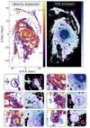 |
Fig. 7. Velocity dispersion and FUV emission. Visual inspection of spatial correlation of velocity dispersion (σeff the colorbar represents units of km s−1) and FUV emission as an indicator of star formation (in units of mJy arcsec−2). The FUV emission is the same GALEX FUV map as shown by Bigiel et al. (2010a). We defined 6 individual sub-regions in the ring, southern area, southern and northern arm, based on where we see either stronger FUV emission or enhanced velocity dispersion. See Sect. 4.1 for the discussion on the different regions. |
Whether the cause of higher velocity dispersion is feedback (from star formation) or gravity-driven turbulence (gravitational instabilities) is still a matter of debate (see e.g., discussion by Krumholz & Burkhart 2016). Some authors in the literature have found that high velocity dispersion is well correlated with regions of active star formation. However, Krumholz & Burkhart (2016) argue that the correlation itself may be explained by the fact that galaxies with more gas tend to have both higher velocity dispersion and more star formation. In a model combining both star formation feedback and radial transport, Krumholz et al. (2018) have shown that turbulence in galaxy disks can be driven by star formation feedback, radial transport, or a combination of both. Our observational analysis of M 83 shows no clear correlation with star formation, suggesting that radial transport (e.g., Schmidt et al. 2016) could be the reason for enhanced velocity dispersion in the outskirts of M 83.
4.2. The extended H I structure and the companion UGCA 365
The sharp edges of the H I gas distribution, especially in the southern and northern parts of the extended H I disk, were already noticed by Heald et al. 2016 (see their Fig. 17). They consider that this is due to photoionization or ram pressure from the intergalactic medium and specifically ruled out technical issues.
The prominent northern extended arm of M 83 emerges from its western part that curves 180° around to the east. This can be seen best in the observations of Heald et al. (2016) and Koribalski et al. (2018), serving as evidence that M 83 may have interacted or merged with another smaller galaxy. In our observations the eastern part of the extended arm is not detected, and the irregular galaxy NGC 5264 is not in our field of view (see Figs. B.1 and C.1). Koribalski et al. (2018) mentioned a clump marking a kink in the northwest side of the arm. We also observed it and refer to it as the “inflection point” because it is also visible in the velocity and residual maps where the velocities change4, and we witnessed enhanced FUV emission at this location (see region 1 in Fig. 7). We marked this inflection point in Fig. 8 along with the northern arm. In the enclosed snapshot made using a 3D viewer tool5, the dwarf irregular galaxy UGCA 365 can be seen in the northernmost region of our field of view (∼55 kpc north of the center of M 83). Its TRGB distance is similar to that of M 83 within the given uncertainty: 5.25 ± 0.42 Mpc (Karachentsev et al. 2007). Koribalski et al. (2018) noted that both, the stellar and the gas distribution show some extension to the southeast along the minor axis of the galaxy and suggested that it may be due to tidal interaction with M 83. In Fig. 8, we denote a ∼20 kpc-long speculative connecting branch between the inflection point and UGCA 365. We detected a faint H I emission close to the inflection point in the direction of this branch. The inflection point is best seen in panel 2 as well as in the zoomed-in version, where it appears to deviate from the general direction of the northern arm. In general, these panels show the warped nature of M 83’s super-extended H I disk.
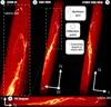 |
Fig. 8. Intensity map of M 83 from different angles showing the northern arm in a 3D viewer tool (see Sect. 4.2). In the two left plots, the arrow pointing west is directed towards us. In the right plot, it is pointing away from us. The northern orientation is the same in both plots. The v direction indicates the velocity axis over which we integrate for the integrated intensity map shown in Fig. 1. The white doted line shows the direction of the northern arm, while the pink dotted line shows the ∼20 kpc long speculative connecting branch to UGCA 365. |
5. Upper limits for average radial mass flow rates in M83
Mass flows – inflow and outflow – play an important role in the process of the evolution of a galaxy. For example, mass flows fuel the inner central molecular zones with fresh, new star-forming material (e.g., Kormendy & Kennicutt 2004 or Henshaw et al. 2022 for the central molecular zone of the Milky Way). In this section, we discuss mass flow rates, their limitations, and how they depend on initial disk parameters.
5.1. Mass flow profile – A simple view
For average mass flow rate profiles across the H I disk in M 83, we used a simplified approach presented, for example, in Di Teodoro & Peek (2021):
![$$ \begin{aligned} \frac{\dot{M}_{\rm HI}(r)}{[M_{\odot }~\mathrm{yr} ^{-1}]} = \frac{2\pi ~r}{\mathrm{[pc]} } \frac{\Sigma _ \mathrm{HI} (r)}{[M_{\odot }~\mathrm{pc} ^{-2}]}~\frac{V_{\rm rad} (r)}{[\mathrm{pc~yr} ^{-1}]}, \end{aligned} $$](/articles/aa/full_html/2023/07/aa45290-22/aa45290-22-eq62.gif)
where the radial velocity profile Vrad(r) and H I surface density profile ΣHI(r) are used to obtain H I mass flow rate profiles. To get radial velocities, Vrad, we used Eq. (12). We restate that Vrad < 0 indicates inflow and Vrad > 0 indicates outflow for M 83 (see Sect. 2.4).
We show the mass flow rate profile in Fig. 9, and also note the radial range of the central disk and ring. Heald et al. (2016) noticed that beyond a radius of ∼22 kpc (they quote 1000″) the approaching and receding side rotation curves differ, and thus, they should not be overinterpreted. Therefore, we shaded the region where the gas distribution and kinematics are no longer symmetric (i.e., deviation from pure circular motions).
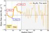 |
Fig. 9. Mass flow rates. Negative (positive) values mean inflow (outflow). We indicate the vertical line where the symmetry in our observed velocities is no longer valid and thus inferred the mass flow rates (beyond galactocentric radius of 23 kpc). We denote the approximate mass flow rates. The peaks and dips are indications in which radial bin in M 83 gas moves to the previous or following radial bin. |
Based on Eq. (13), we found within the central disk (i) at radii ∼2 kpc evidence of outflowing material with mass flow rates of ∼1 M⊙ yr−1 and (ii) at r ∼ 5.5 kpc inflowing material of ∼2 M⊙ yr−1. We found indications of (iii) outflowing material of the order ∼10 M⊙ yr−1 at radii of r ∼ 14 kpc, that is the ring (see mask in Fig. 5). In this region, we also found higher residual velocities. Moreover, using the Vlos, obs map, we found enhanced velocity dispersion compared to the edges of the central disk of ∼20 km s−1 in that same ring region (median value; σeff and  , see Fig. 6).
5.2. Initial parameters and their impact on ring-averaged mass flow rates
Multiple variants of tilted ring codes exist in the literature, for example, the 2D fitter GIPSY task rotcur (Begeman 1989) and the 3D fitter BBarolo (Di Teodoro & Fraternali 2015) and FAT (Kamphuis et al. 2015). After running these codes, the next step is often to interpret the noncircular motions and relate them, for example, to flow motions and/or interactions with a companion galaxy. M 83 provides one of the best cases, as it has different kinematic parameters available in the literature.
In Fig. 10, we show another recently published set of kinematic parameters of M 83, which includes position angle, inclination, Vrot, and Vrad with observations from LVHIS using BBarolo (by Di Teodoro & Peek 2021; extracted from their appendix Fig. 15 for M 83, also known as NGC 5236). That is the same work from which we adopted the simplified method to derive mass flow rates (see Eq. (13)). Their tilted rings, however, only extend to rgal = 30 kpc and therefore do not include the southern and northern extended arms. We show the resulting residual velocity maps of both sets of kinematic parameters and how we interpolated the tilted rings (only for visual purposes) in Fig. 11. When comparing the two Vres maps, we saw no great difference in the inner disk. In the residual map of Di Teodoro & Peek (2021), the deviations of the circular motions in the ring region are smaller than in the one of Heald et al. (2016). In the southern area, we observed the opposite behavior: higher deviations of circular motions in the Vres map of Di Teodoro & Peek (2021). We took Di Teodoro & Peek’s kinematic parameters shown in Fig. 10 and fit them with the same procedure we used for the kinematic parameters from Heald et al. (2016; see Sect. 2.4). After the fitting, we again calculated the mass flow rate using Eq. (13).
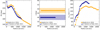 |
Fig. 10. Parameter comparison. In orange we show the kinematic parameters we used in this work for the velocity field shown in Sect. 3.2. In Sect. 5.2 we investigate how different initial parameters affect mass flow rates using the approach from Di Teodoro & Peek (2021) using their own set of parameters for M 83 (blue markers). |
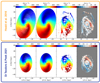 |
Fig. 11. Comparison of residual maps. Here we compare the modeled and residual maps (Vlos, mdl and Vres) of different initial parameters (shown in Fig. 10) that we obtained by using Eq. (8). Upper row: the tilted rings using (Heald et al. 2016) model outputs that are based on their KAT7 observations and using rotcurv. For visualisation reasons, we interpolated the gaps using the scipy function 2d interpolation. For further analysis we focus on the tilted-ring frame. Lower row: the tilted rings using (Di Teodoro & Peek 2021) model outputs that are based on LVHIS observations and using BBarolo. The field of view is restricted to their Vrot parameters. Therefore the southern and northern arm are not evident in the residual map. |
We show the two average radial mass flow rate profiles in Fig. 12. What is immediately noticeable is that the two are drastically different. In the ring region, they even indicate the opposite trend – inflowing material. Di Teodoro & Peek (2021) found a lower inclination, i = 40° compared to i = 48°. The differences in position angle shift the minor axis, and with the lower inclination, they led to a flip in the inferred flow direction: from outflow to inflow. Additionally, also using LVHIS observations, Kamphuis et al. (2015) derived kinematic parameters using 3D fitting FAT and obtained an inclination value of i = 40.3°6 for M 83. In other words, Kamphuis et al. (2015) and Di Teodoro & Peek (2021) found similar lower values for the inclination than Heald et al. (2016).
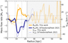 |
Fig. 12. Mass flow rate of this work (orange) and mass flow rate using different initial parameters as shown in Fig. 10 (blue). The dashed lines show Vrad. Negative (positive) values mean inflow (outflow). Within the ring region we find the opposite trend of mass flow rates. We discuss the reasons for this in Sect. 5.2. |
However, Heald et al. (2016) also determined kinematic parameters using the THINGS data (presented by de Blok et al. 2008) and obtained higher values for the inclination, i = 46°. For this purpose, they used the 2D fitting routine rotcur. This higher inclination value and the one derived from the KAT7 observations (i.e., i = 46° and i = 48°, respectively) agree better with the isophote orientations in the optical disk.
This is a good demonstration of how challenging it is to unambiguously determine inflow and outflow rates. The inclination depends on whether the kinematics are fitted with 2D or 3D tilted rings (BBarolo tends to fit incliniations 10° lower than 2D fitters; Di Teodoro & Fraternali 2015). Even at inclinations that are far from being face on, the chosen inclination can have a large impact on the inferred mass flow rate. Mass flow rates are sensitive to inclination and position angle to the extent that inflows can even flip signs. At the same point, mass flow rates seem not to be sensitive to the employed 3D fit (adopted by Di Teodoro & Peek 2021) or 2D fit (used here). Also, “circular motion plus axisymmetric radial motion” (see Eq. (7)) is not guaranteed to yield the true inflow rate if the Vrot + Vrad model is not accurate. For these reasons, the values given in Figs. 9 and 12 should be considered with caution, though we point out that they do represent our best guess at the H I mass flow rates and directions in M 83.
In the velocity fields (Fig. 4) and in Fig. 8, we witnessed the warped nature of M83’s super-extended H I disk. The position angle twists by almost 90° from the orientation of the central disk. As mentioned by Heald et al. (2016), this shift in isovelocity was accounted by letting the vsys parameter change in their models (which we adopted in this work; see Sect. 2.6.1). However, it has been shown that bar streaming motions are hard to neglect when analyzing mass flow rates toward the Milky Way’s central molecular zone (e.g., Kim et al. 2012; Sormani et al. 2015; Sormani & Barnes 2019; Tress et al. 2020) or in nearby galaxies (e.g., Erroz-Ferrer et al. 2015; Salak et al. 2019). The M 83 galaxy is cataloged as SAB(s)c (see Table 1) – in between the classifications of a barred spiral galaxy and an unbarred spiral galaxy. The bar within M 83’s central disk is the main reason for the gas inflow seen at r ∼ 5.5 kpc; thus, the inferred inflow rates at these radii might be underestimated. However, both mass flow rate profiles shown in Fig. 12 are consistent for these small radii that cover the bar.
5.3. Interpreting mass flow rates in M 83
Keeping the uncertainties in mind, the following discussion is based on an approximation of the upper limits of the mass flow rates in M 83. We compare our results (presented in Fig. 9) to multi-wavelength literature studies (i.e., further evidence for mass flows) to interpret our findings.
Starting from the very center of M 83, a study identified signatures of inflowing gas toward its inner circumnuclear ring (∼130 pc in radius) using ALMA HCN(1–0) and HCO+(1–0) observations (Callanan et al. 2021). Recently published results toward M 83’s optical disk using Multi-unit spectroscopic explorer (MUSE) observations have shown indications of outflowing ionized gas (Della Bruna et al. 2022). This flow is east of M 83’s nucleus and ∼1.2 kpc7 in size. This could be consistent with our H I observations indicating an outflow at a galactocentric radius of ∼2 kpc.
The kinematics over the whole central optical disk of M 83 have been studied, for example, in Lundgren et al. (2004) and Fathi et al. (2008). Lundgren et al. (2004) found molecular streaming motions along the spiral arms when using CO(2–1) and CO(1–0) observations. These motions start at rgal ∼ 5.6 kpc8 toward M 83’s center. This observation agrees with our potential (ii) inflow at r ∼ 5.5 kpc. Fathi et al. (2008) confirmed this spiral inflow using Fabry-Perot observations of the Hα line across the inner ∼2.3 kpc of the central disk, capturing this inflow down to a few tens of parsecs from the dynamical nucleus of M 83. For the possible outflowing material in the outermost region at radii of rgal ∼ 14 kpc, we found no correspondence in the literature.
From a theoretical point of view, gas is most likely to first accrete onto galaxies at larger radii and then move radially toward the inner disk to feed star formation (e.g., Ho et al. 2019). Cosmological hydrodynamical simulations of Milky Way-like galaxies have shown expected gas inflow of a few km s−1 within the inner optical disk that reaches ∼10 km s−1 in the outskirts (e.g., Trapp et al. 2022). Trapp et al. (2022) also found that the gas accumulates at the disk edge and then decreases in average radial speed and increases in column density. Observations also show similar inflow velocities of a few km s−1. For example, Wong et al. (2004) decomposed H I and CO velocity fields of concentric elliptical rings into a third-order Fourier series for seven nearby spiral galaxies. Schmidt et al. (2016) performed a Fourier decomposition of velocity fields for ten THINGS galaxies. Both of these studies found ring-averaged radial inflow velocities of 5 − 10 km s−1 and 5 − 20 km s−1, respectively, though they used methods different from those in this study. In these models and observations, radial velocities of more than 40 km s−1 have not been observed.
In our ring region in M 83, the high values (see right y axis in Fig. 12) are most likely due to differences in the adopted inclination values. The mass inflow rate is strongly dependent on the determined geometry of a galaxy, and therefore, it is hard to make clear estimates of how many solar masses are transported to M83’s central disk. However, we observed ≈1.9 × 10⁹ M⊙ of gas at a distance of 16 kpc9 from the center with a circular orbital period of 4.46 × 10³ Myr10. To reach inflow rates of 10 M⊙ per year would require infall on a timescale of ∼2.0 × 10⁴ Myr, which is four times that of an orbital time or 0.7 of a free fall time11.
6. Conclusion
In this paper, we have investigated the super-extended H I disk of M 83 based on ten pointing VLA observations at 21″ (≈500 pc) angular resolution. We found the following:
-
We detected significant H I emission until a radius of ∼50 kpc. The most prominent features in Fig. 1 are the northern extended arm, the southern arm, and the ring surrounding the central disk.
-
To investigate noncircular motions, we adopted tilted-model outputs from Heald et al. (2016) based on KAT7 observations. We find the highest deviations to be from pure circular motion in the ring (see Fig. 4).
-
We examined environmental differences in velocities (Vlos and Vres), atomic gas surface density (ΣHI), and velocity dispersion (σ). To that end, we defined independent regions: central disk, ring, southern area, southern arm, and northern arm. Based on Fig. 5, we find that overall ΣHI and σ decrease with galactocentric radius, in agreement with prior work. The distribution of Vres toward the ring and northern arm shows a second peak of −25 km s−1.
-
We examined the radial and environmental dependence of velocity dispersion across the whole disk of M 83. We analyzed the velocity dispersion, σ, using the effective-width (σeff) and second-moment (
 ) approaches (see Fig. 6). We find enhanced velocity dispersion in the ring as well as in the central disk using both techniques. This indicates that the atomic gas in the ring region seems to be more turbulent than in the outer regions.
 -
We compared σ with FUV emission to trace recent star formation. We did not find enhanced FUV emission where we found enhanced H I velocity dispersion. This anticorrelation with star formation suggests that radial transport could be the reason for enhanced velocity dispersion in the outskirts of M 83 (see Fig. 7).
-
We found an “inflection point” in the observed velocities along the northern arm and speculate a possible connecting branch to the dwarf irregular galaxy UGCA 365 that deviates from the general direction of the northern arm (see Fig. 8).
-
We used a simplified model to obtain a radial mass flow rate profile and compared it with the mass flow rates in the literature. We showed that kinematic parameters have a strong impact on these profiles. Although mass inflow is one of the most important processes feeding star formation, tilted ring models (2D or 3D) as the basis for deriving such profiles, are strongly sensitive to initial parameters (see e.g., Fig. 12). Furthermore, warped or flaring H I disks or distinct features at large radii further complicate the derivation of the kinematic parameters. To investigate this in more detail, more sophisticated models are needed to correctly determine the kinematics of this extended structure.
-
In agreement with recent studies, we find within the central disk hints of inflowing material close to the nuclear region and outflowing material in the outer areas of the central disk.
The central disk and the ring were masked by a radius cut (rgal = 8.1 kpc and rgal = 16 kpc, respectively) in the plane of the disk. The gap between the central disk and the ring represents lines of sight that were difficult to assign to a specific region, and thus they were not included in a region. The two arms and the southern area were selected with a cut in RA and declination.
We do not show the calculated mass flow rates for the inclination value given in Kamphuis et al. (2015), as they did not provide any tables or radial plots for their position angles from which we would be able to extract them.
We use here and in the following a distance of 5.16 Mpc, the same mentioned in Table 1, to get physical scales.
Assuming that the ring mass (with average surface density ∼3 M⊙/pc2 adopted from Fig. 5) is distributed over an 8 kpc-wide area (i.e., the width of the ring, rgal = ∼8 − 16 kpc).
By taking the average Vrot at the ring radius ∼160 km s−1 from Fig. 10.
If we take torb ∼ 6 tff; see Eq. (E).
Acknowledgments
We would like to thank the anonymous referee for their insightful comments that helped improve the quality of the paper. CE gratefully acknowledges funding from the Deutsche Forschungsgemeinschaft (DFG) Sachbeihilfe, grant number BI1546/3-1. CE, FB, AB, IB, JdB and JP acknowledge funding from the European Research Council (ERC) under the European Union’s Horizon 2020 research and innovation programme (grant agreement No.726384/Empire). The work of AKL is partially supported by the National Science Foundation under Grants No. 1615105, 1615109, and 1653300. ER acknowledges the support of the Natural Sciences and Engineering Research Council of Canada (NSERC), funding reference number RGPIN-2017-03987. TGW acknowledges funding from the European Research Council (ERC) under the European Union’s Horizon 2020 research and innovation programme (grant agreement No. 694343). JMDK gratefully acknowledges funding from the European Research Council (ERC) under the European Union’s Horizon 2020 research and innovation programme via the ERC Starting Grant MUSTANG (grant agreement number 714907). COOL Research DAO is a Decentralised Autonomous Organisation supporting research in astrophysics aimed at uncovering our cosmic origins. SCOG acknowledges funding from the European Research Council via the ERC Synergy Grant “ECOGAL – Understanding our Galactic ecosystem: From the disk of the Milky Way to the formation sites of stars and planets” (project ID 855130), from the Deutsche Forschungsgemeinschaft (DFG) via the Collaborative Research Center (SFB 881 – 138713538) “The Milky Way System” (subprojects A1, B1, B2 and B8) and from the Heidelberg Cluster of Excellence (EXC 2181 – 390900948) “STRUCTURES: A unifying approach to emergent phenomena in the physical world, mathematics, and complex data”, funded by the German Excellence Strategy. MQ acknowledges support from the Spanish grant PID2019-106027GA-C44, funded by MCIN/AEI/10.13039/501100011033. KG is supported by the Australian Research Council through the Discovery Early Career Researcher Award (DECRA) Fellowship DE220100766 funded by the Australian Government. HH acknowledges the support of the Natural Sciences and Engineering Research Council of Canada (NSERC), funding reference number RGPIN-2017-03987 and the Canadian Space Agency funding reference 21EXPUVI3. EW is funded by the Deutsche Forschungsgemeinschaft (DFG, German Research Foundation) – Project-ID 138713538 – SFB 881 (“The Milky Way System”, subproject P2). WJGdB received funding from the European Research Council (ERC) under the European Union’s Horizon 2020 research and innovation programme (grant agreement No 882793 ‘MeerGas’). D.J.P. is supported through the South African Research Chairs Initiative of the Department of Science and Technology and National Research Foundation and acknowledges partial support from NSF CAREER grant AST-1149491. This work is based on observations carried out with the Karl G. Jansky Very Large Array (VLA) and the Green Bank Telescope (GBT). The National Radio Astronomy Observatory is a facility of the National Science Foundation operated under cooperative agreement by Associated Universities, Inc. The Green Bank Observatory is a facility of the National Science Foundation operated under cooperative agreement by Associated Universities, Inc. This work is based in part on observations made with the Galaxy Evolution Explorer (GALEX). GALEX is a NASA Small Explorer, whose mission was developed in cooperation with the Centre National d’Etudes Spatiales (CNES) of France and the Korean Ministry of Science and Technology. GALEX is operated for NASA by the California Institute of Technology under NASA contract NAS5-98034. Software: NumPy (Harris et al. 2020), SciPy (Virtanen et al. 2020), Astropy (Astropy Collaboration 2018), pandas (The pandas development team 2021), Matplotlib (Hunter 2007), CASA (CASA Team 2022), BBarolo (EdT & Oman 2021), rotcur (Begeman 1989), radio-astro-tools (uvcombine) (Koch & Ginsburg 2022), glnemo2 (https://projets.lam.fr/projects/glnemo2/wiki/) astrometry (https://nova.astrometry.net/)
References
- Astropy Collaboration (Robitaille, T. P., et al.) 2013, A&A, 558, A33 [NASA ADS] [CrossRef] [EDP Sciences] [Google Scholar]
- Astropy Collaboration (Price-Whelan, A. M., et al.) 2018, AJ, 156, 123 [Google Scholar]
- Begeman, K. G. 1989, A&A, 223, 47 [NASA ADS] [Google Scholar]
- Bešlić, I., Barnes, A. T., Bigiel, F., et al. 2021, MNRAS, 506, 963 [CrossRef] [Google Scholar]
- Bialy, S., & Sternberg, A. 2019, ApJ, 881, 160 [NASA ADS] [CrossRef] [Google Scholar]
- Bigiel, F., Leroy, A., Seibert, M., et al. 2010a, ApJ, 720, L31 [NASA ADS] [CrossRef] [Google Scholar]
- Bigiel, F., Leroy, A., Walter, F., et al. 2010b, AJ, 140, 1194 [NASA ADS] [CrossRef] [Google Scholar]
- Callanan, D., Longmore, S. N., Kruijssen, J. M. D., et al. 2021, MNRAS, 505, 4310 [NASA ADS] [CrossRef] [Google Scholar]
- CASA Team (Bean, B., et al.) 2022, PASP, 134, 114501 [NASA ADS] [CrossRef] [Google Scholar]
- Cornwell, T. J. 2008, IEEE J. Sel. Top. Signal Proc., 2, 793 [NASA ADS] [CrossRef] [Google Scholar]
- de Blok, W. J. G., Walter, F., Brinks, E., et al. 2008, AJ, 136, 2648 [NASA ADS] [CrossRef] [Google Scholar]
- de Blok, W. J. G., Adams, E. A. K., Amram, P., et al. 2016, Proc. MeerKAT Science: On the Pathway to the SKA, 25-27 May, 2016 Stellenbosch, South Africa (MeerKAT2016), online at https://pos.sissa.it/cgi-bin/reader/conf.cgi?confid=277, 7 [Google Scholar]
- Della Bruna, L., Adamo, A., Amram, P., et al. 2022, A&A, 660, A77 [NASA ADS] [CrossRef] [EDP Sciences] [Google Scholar]
- de Vaucouleurs, G., de Vaucouleurs, A., Corwin, H. G. J., et al. 1991, Third Reference Catalogue of Bright Galaxies [Google Scholar]
- Dickey, J. M., Strasser, S., Gaensler, B. M., et al. 2009, ApJ, 693, 1250 [NASA ADS] [CrossRef] [Google Scholar]
- Di Teodoro, E. M., & Fraternali, F. 2015, MNRAS, 451, 3021 [Google Scholar]
- Di Teodoro, E. M., & Peek, J. E. G. 2021, ApJ, 923, 220 [NASA ADS] [CrossRef] [Google Scholar]
- EdT,& Oman, K. 2021, https://doi.org/10.5281/zenodo.5510565 [Google Scholar]
- Erroz-Ferrer, S., Knapen, J. H., Leaman, R., et al. 2015, MNRAS, 451, 1004 [NASA ADS] [CrossRef] [Google Scholar]
- Fathi, K., Beckman, J. E., Lundgren, A. A., et al. 2008, ApJ, 675, L17 [NASA ADS] [CrossRef] [Google Scholar]
- Field, G. B., Goldsmith, D. W., & Habing, H. J. 1969, ApJ, 155, L149 [NASA ADS] [CrossRef] [Google Scholar]
- Harris, C. R., Millman, K. J., van der Walt, S. J., et al. 2020, Nature, 585, 357 [NASA ADS] [CrossRef] [Google Scholar]
- Heald, G., Józsa, G., Serra, P., et al. 2011, A&A, 526, A118 [NASA ADS] [CrossRef] [EDP Sciences] [Google Scholar]
- Heald, G., de Blok, W. J. G., Lucero, D., et al. 2016, MNRAS, 462, 1238 [NASA ADS] [CrossRef] [Google Scholar]
- Henshaw, J. D., Barnes, A. T., Battersby, C., et al. 2022, ArXiv e-prints [arXiv:2203.11223] [Google Scholar]
- Heyer, M. H., Carpenter, J. M., & Snell, R. L. 2001, ApJ, 551, 852 [NASA ADS] [CrossRef] [Google Scholar]
- Ho, S. H., Martin, C. L., & Turner, M. L. 2019, ApJ, 875, 54 [NASA ADS] [CrossRef] [Google Scholar]
- Huchtmeier, W. K., & Bohnenstengel, H. D. 1981, A&A, 100, 72 [NASA ADS] [Google Scholar]
- Hunter, J. D. 2007, Comput. Sci. Eng., 9, 90 [NASA ADS] [CrossRef] [Google Scholar]
- Ianjamasimanana, R., de Blok, W. J. G., Walter, F., & Heald, G. H. 2012, AJ, 144, 96 [NASA ADS] [CrossRef] [Google Scholar]
- Ianjamasimanana, R., de Blok, W. J. G., Walter, F., et al. 2015, AJ, 150, 47 [NASA ADS] [CrossRef] [Google Scholar]
- Jameson, K. E., McClure-Griffiths, N. M., Liu, B., et al. 2019, ApJS, 244, 7 [NASA ADS] [CrossRef] [Google Scholar]
- Jiménez-Donaire, M. J., Bigiel, F., Leroy, A. K., et al. 2019, ApJ, 880, 127 [CrossRef] [Google Scholar]
- Kamphuis, P., Józsa, G. I. G., Oh, S. H., et al. 2015, MNRAS, 452, 3139 [NASA ADS] [CrossRef] [Google Scholar]
- Karachentsev, I. D., Tully, R. B., Dolphin, A., et al. 2007, AJ, 133, 504 [NASA ADS] [CrossRef] [Google Scholar]
- Kepley, A. A., Tsutsumi, T., Brogan, C. L., et al. 2020, PASP, 132, 024505 [Google Scholar]
- Kereš, D., Katz, N., Weinberg, D. H., & Davé, R. 2005, MNRAS, 363, 2 [Google Scholar]
- Kim, W.-T., Seo, W.-Y., Stone, J. M., Yoon, D., & Teuben, P. J. 2012, ApJ, 747, 60 [Google Scholar]
- Koch, E., & Ginsburg, A. 2022, Astrophysics Source Code Library [record ascl:2208.014] [Google Scholar]
- Koch, E. W., Rosolowsky, E. W., Lockman, F. J., et al. 2018, MNRAS, 479, 2505 [NASA ADS] [CrossRef] [Google Scholar]
- Koch, E. W., Rosolowsky, E. W., Leroy, A. K., et al. 2021, MNRAS, 504, 1801 [NASA ADS] [CrossRef] [Google Scholar]
- Koda, J., Sawada, T., Sakamoto, K., et al. 2020, ApJ, 890, L10 [NASA ADS] [CrossRef] [Google Scholar]
- Koribalski, B. S., Wang, J., Kamphuis, P., et al. 2018, MNRAS, 478, 1611 [NASA ADS] [CrossRef] [Google Scholar]
- Kormendy, J., & Kennicutt, Jr., R. C. 2004, ARA&A, 42, 603 [NASA ADS] [CrossRef] [Google Scholar]
- Krumholz, M. R., & Burkhart, B. 2016, MNRAS, 458, 1671 [NASA ADS] [CrossRef] [Google Scholar]
- Krumholz, M. R., Burkhart, B., Forbes, J. C., & Crocker, R. M. 2018, MNRAS, 477, 2716 [CrossRef] [Google Scholar]
- Lambert, J. C. 2012, in Astronomical Data Analysis Software and Systems XXI, eds. P. Ballester, D. Egret, & N. P. F. Lorente, ASP Conf. Ser., 461, 897 [NASA ADS] [Google Scholar]
- Leroy, A. K., Hughes, A., Schruba, A., et al. 2016, ApJ, 831, 16 [Google Scholar]
- Leroy, A. K., Sandstrom, K. M., Lang, D., et al. 2019, ApJs, 244, 24 [NASA ADS] [CrossRef] [Google Scholar]
- Leroy, A. K., Schinnerer, E., Hughes, A., et al. 2021, ApJs, 257, 43 [NASA ADS] [CrossRef] [Google Scholar]
- Lundgren, A. A., Olofsson, H., Wiklind, T., & Rydbeck, G. 2004, A&A, 422, 865 [NASA ADS] [CrossRef] [EDP Sciences] [Google Scholar]
- McMullin, J. P., Waters, B., Schiebel, D., Young, W., & Golap, K. 2007, in Astronomical Data Analysis Software and Systems XVI, eds. R. A. Shaw, F. Hill, & D. J. Bell, ASP Conf. Ser., 376, 127 [Google Scholar]
- Miller, E. D., Bregman, J. N., & Wakker, B. P. 2009, ApJ, 692, 470 [NASA ADS] [CrossRef] [Google Scholar]
- Mogotsi, K. M., de Blok, W. J. G., Caldú-Primo, A., et al. 2016, AJ, 151, 15 [NASA ADS] [CrossRef] [Google Scholar]
- Oh, S.-H., Kim, S., For, B.-Q., & Staveley-Smith, L. 2022, ApJ, 928, 177 [NASA ADS] [CrossRef] [Google Scholar]
- Oman, K. A., Marasco, A., Navarro, J. F., et al. 2019, MNRAS, 482, 821 [NASA ADS] [CrossRef] [Google Scholar]
- Pingel, N. M., Pisano, D. J., Heald, G., et al. 2018, ApJ, 865, 36 [NASA ADS] [CrossRef] [Google Scholar]
- Pisano, D. J. 2014, AJ, 147, 48 [NASA ADS] [CrossRef] [Google Scholar]
- Rogstad, D. H., Lockhart, I. A., & Wright, M. C. H. 1974, ApJ, 193, 309 [Google Scholar]
- Romeo, A. B., & Mogotsi, K. M. 2017, MNRAS, 469, 286 [NASA ADS] [CrossRef] [Google Scholar]
- Rosolowsky, E., & Leroy, A. 2006, PASP, 118, 590 [NASA ADS] [CrossRef] [Google Scholar]
- Salak, D., Noma, Y., Sorai, K., et al. 2019, PASJ, 71, S16 [NASA ADS] [Google Scholar]
- Sancisi, R., Fraternali, F., Oosterloo, T., & van der Hulst, T. 2008, A&ARv, 15, 189 [NASA ADS] [CrossRef] [Google Scholar]
- Sardone, A., Pisano, D. J., Pingel, N. M., et al. 2021, ApJ, 910, 69 [NASA ADS] [CrossRef] [Google Scholar]
- Schmidt, T. M., Bigiel, F., Klessen, R. S., & de Blok, W. J. G. 2016, MNRAS, 457, 2642 [NASA ADS] [CrossRef] [Google Scholar]
- Sormani, M. C., & Barnes, A. T. 2019, MNRAS, 484, 1213 [NASA ADS] [CrossRef] [Google Scholar]
- Sormani, M. C., Binney, J., & Magorrian, J. 2015, MNRAS, 449, 2421 [NASA ADS] [CrossRef] [Google Scholar]
- Stanimirovic, S., Staveley-Smith, L., Dickey, J. M., Sault, R. J., & Snowden, S. L. 1999, MNRAS, 302, 417 [CrossRef] [Google Scholar]
- Stilp, A. M., Dalcanton, J. J., Warren, S. R., et al. 2013a, ApJ, 765, 136 [NASA ADS] [CrossRef] [Google Scholar]
- Stilp, A. M., Dalcanton, J. J., Skillman, E., et al. 2013b, ApJ, 773, 88 [NASA ADS] [CrossRef] [Google Scholar]
- Sun, J., Leroy, A. K., Schruba, A., et al. 2018, ApJ, 860, 172 [NASA ADS] [CrossRef] [Google Scholar]
- Tamburro, D., Rix, H. W., Leroy, A. K., et al. 2009, AJ, 137, 4424 [Google Scholar]
- The pandas development team 2021, https://github.com/pandas-dev/pandas [Google Scholar]
- Thilker, D. A., Bianchi, L., Boissier, S., et al. 2005, ApJ, 619, L79 [Google Scholar]
- Tilanus, R. P. J., & Allen, R. J. 1993, A&A, 274, 707 [NASA ADS] [Google Scholar]
- Trapp, C. W., Kereš, D., Chan, T. K., et al. 2022, MNRAS, 509, 4149 [Google Scholar]
- Tress, R. G., Sormani, M. C., Glover, S. C. O., et al. 2020, MNRAS, 499, 4455 [NASA ADS] [CrossRef] [Google Scholar]
- Tumlinson, J., Peeples, M. S., & Werk, J. K. 2017, ARA&A, 55, 389 [Google Scholar]
- Utomo, D., Blitz, L., & Falgarone, E. 2019, ApJ, 871, 17 [NASA ADS] [CrossRef] [Google Scholar]
- Virtanen, P., Gommers, R., Oliphant, T. E., et al. 2020, Nat. Methods, 17, 261 [Google Scholar]
- Walter, F., Brinks, E., de Blok, W. J. G., et al. 2008, AJ, 136, 2563 [Google Scholar]
- Wang, J., Koribalski, B. S., Serra, P., et al. 2016, MNRAS, 460, 2143 [Google Scholar]
- Warren, S. R., Skillman, E. D., Stilp, A. M., et al. 2012, ApJ, 757, 84 [NASA ADS] [CrossRef] [Google Scholar]
- White, S. D. M., & Frenk, C. S. 1991, ApJ, 379, 52 [Google Scholar]
- Wolfire, M. G., Hollenbach, D., McKee, C. F., Tielens, A. G. G. M., & Bakes, E. L. O. 1995, ApJ, 443, 152 [Google Scholar]
- Wolfire, M. G., McKee, C. F., Hollenbach, D., & Tielens, A. G. G. M. 2003, ApJ, 587, 278 [Google Scholar]
- Wong, T., Blitz, L., & Bosma, A. 2004, ApJ, 605, 183 [NASA ADS] [CrossRef] [Google Scholar]
Appendix A: Image Combination
Similar to the procedure described in the appendix of Koch et al. (2018), itself based on Chapter 3 of Stanimirovic et al. (1999), we analyzed the effects of combining the (i) VLA data with single dish (ii) Green Bank Telescope (GBT; project GBT11A-055) observations. (i) The VLA observation has an angular resolution of 21″ (∼500 pc) and a spectral resolution of 5.0 km s−1. (ii) The GBT observation has an angular resolution of 523″ (∼12.13 kpc) and a spectral resolution of 5.15 km s−1 (see Figure A.1, panel 1a).
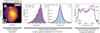 |
Fig. A.1. Image combination. (a) We show the integrated intensity maps of the GBT observation at native angular resolution. (b) Shows the distribution of the flux of the single dish (SD) and VLA data at matched spectral resolution (i.e. we regridded the VLA to the GBT spectral resolution). (c): We used the uvcombine python package to find the single dish scaling factor (sdf; blue line). The ratio of the low-res and high-res observations result in a Cauchy distribution. We fit the log of the ratio to a Cauchy distribution (blue histogram) and its mean is then an estimate for the scaling factor. (d): The spectra of the VLA and GBT observation at matched angular and spectral resolution (i.e. we gaussian convolve and regridded the VLA to the GBT angular and spectral resolution). |
We used a distribution-based method on the u − v-amplitudes where the spatial coverage of the VLA and single dish data overlap to quantify the scaling factor. We used the uvcombine package (Koch & Ginsburg 2022) and examined the distributions of the single dish amplitudes, the VLA amplitudes, and their ratio across all channels. The amplitudes of the single dish and VLA in the overlap regions are well described by normal distributions, and as such, the ratio of the log-amplitude follows a Cauchy distribution (Koch et al. 2018). We fit a Cauchy distribution and used the location of the peak of the distribution as the scale factor. In Figure A.1, panel 1c, we show the distribution of the amplitudes across all channels and the best-fit Cauchy distribution.
Adopting a maximum-likelihood approach and using the ratios from all channels, we found a scaling factor of 0.982±0.003 for the GBT data. Because we expected the absolute flux uncertainties to be ∼10%, the scaling factor from the distribution fit is consistent with one, and thus we did not apply a scaling factor to the GBT data before feathering.
Appendix B: Ten mosaic pointing and channel maps
The coordinates of the 10-point mosaic of our VLA observation that are shown in Figure B.1.
Figure B.1 shows the ten mosaic pointing for our VLA observation. We show the positions and their corresponding coordinates.
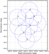 |
Fig. B.1. The position for the extended (∼1.52 deg) 10-point mosaic of our VLA observation. |
In Eq. (B.2) we show all channels (contrary to the overview shown in Figure 2, where we took every third 5.0 km s−1 channel) of our imaged data set. During the imaging procedure, we chose a spectral resolution of Δv = 5.0 km s−1 to increase the S/N of our observations.
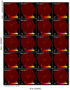 |
Fig. B.2. Channel maps of our VLA+GBT data. Here we show now every 5.0 km s−1 channel. The line-of-sight velocity of the shown channels is displayed on the upper left corner of each panel. |
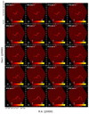 |
Fig. B.2. Continued. |
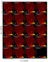 |
Fig. B.2. Continued. |
Appendix C: Green Bank Telescope observation
We show in Figure C.1 the integrated intensity map of the GBT observation with an angular resolution of 523″ together with the field of view of the VLA observation and the location of UGCA 365. The H I emission of UGCA 365 is faint relative to M 83 (∼10 K km s−1 compared to ∼400 K km s−1).
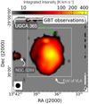 |
Fig. C.1. Integrated intensity map of the GBT observation. The white contours show the field of view of the VLA observation. We denote the companion galaxies UGCA 365 and NGC 5264. The H I emission of UGCA 365 is faint relative to M 83 (∼10 K km s−1 compared to ∼400 K km s−1). |
Appendix D: Multiple velocity components
In Section 4.1 we mentioned that some of our sightlines show non-Gaussian or multiple velocity components. We show four examples in Eq. (D.1). We show in the left panels the velocity dispersion calculated with Eq. (5) and show the hexagon in green, of which we show the spectrum on the right. These spectra represent the multicomponent behavior of the spectrum of individual lines of sight in the ring region.
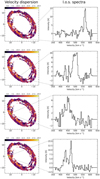 |
Fig. D.1. Examples of four spectra of individual line of sights that show higher values in the velocity map. These show the multi-component behavior of the spectra. |
We looked into individual regions and compared the two approaches discussed in this paper to derive the velocity dispersion (i.e., σeff and  ) in Figure D.2. In the figure, we show linear regression fits in the form of log(y) = β × log(x)+α. We found for the central disk and ring region a moderate12 linear correlation between σeff and
  . For all the other regions, we found a weak, approximately linear correlation. We observed the highest scatter in
  in the ring region of ∼2.5 dex, followed by a scatter of ∼2.0 dex toward the central disk and southern area. These scatters most likely highlight the multicomponent and/or wider components of a spectrum. In the first panel of Figure D.2, where we show the x and y axis in linear scales, the velocity dispersions over ∼20 km s−1 are likely to represent a multicomponent spectrum.
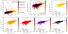 |
Fig. D.2. Comparison of two approaches to determine the velocity dispersion. In all panels, the y-axes show the |


Appendix E: Orbital time and free fall time
In Section 5.3 we assumed that torb ∼ 6 tff. Here, we show the derivation of that result. We assumed that the material is distributed like a uniform density sphere. Then tff at some radius R within that mass distribution is:
where ρ = M / ((4 π R3)/3) and where M is the mass enclosed within R and can also be expressed in terms of rotational velocities vrot:

The orbital time torb is defined as:
As a result we get:

or

This, however, does not imply that material will undergo free fall to the center since there is a lot of kinetic energy and angular momentum that will prevent it. It nevertheless serves as a good estimate.
All Tables
The coordinates of the 10-point mosaic of our VLA observation that are shown in Figure B.1.
All Figures
|
Fig. 1. Integrated intensity map (moment 0) for H I emission across the disk of M 83 at a resolution of 21″. The black circle in the lower left corner marks the beam size of 21″ (≈500 pc). The black to white colorbar indicates integrated intensities from 0 − 100 K km s1 and the orange to yellow integrated intensities above 101 K km s1. We denote the companion galaxy UGCA 365 which in projection is ∼55 kpc away from the center of M 83. To the right, we show the enclosed optical disk (r25 ∼ 8 kpc) overlaid with H I column density contour (NHI = 13 × 1019 cm−2) extending over a radius of ∼40 kpc. For visualization reasons, we show unfilled NHI contours for the high resolution optical image. Beyond 10 kpc we show filled NHI contours. The white line surrounding M 83 shows the field of view (FoV; i.e. the full mosaic coverage) of the VLA observation. (optical image credits: CTIO/NOIRLab/DOE/NSF/AURA, M. Soraisam; Image processing: Travis Rector, Mahdi Zamani & Davide de Martin; low resolution background > 10 kpc: DSS2). |
| In the text | |
|
Fig. 2. Channel maps of our VLA+GBT data. The line-of-sight velocity of the shown channels is displayed on the upper left corner of each panel and the colorbar is shown in units of K. For visual purpose we only show every third 5.0 km s−1 channel (i.e. we do not integrate over channels). The companion galaxy UGCA 365 is detected in the velocity channels 559 km s−1 and 574 km s−1. We show all channels in the appendix (see Appendix B). |
| In the text | |
|
Fig. 3. Global H I profile of M 83 from our VLA observations (orange) and the results of feathering the VLA with the GBT observations (black). The systemic velocity appropriate for the centre of the galaxy is indicated with the vertical grey dashed line at 510 km s−1 (see also Table 1). We also show H I observations of the same FoV of M 83 from LVHIS (Koribalski et al. 2018) and KAT7 (Heald et al. 2016) that we have sampled on the same spectral axis grid at their native angular resolution. |
| In the text | |
|
Fig. 4. Observed, adopted, and residual velocity maps. Observed: velocity field of M 83 using our VLA H I observations. The blue colors represent the approaching and the red is the receding side of the H I galaxy disk. Adopted tilted ring model: constructed velocity field using Vsys, Vrot, i, and position angle of the tilted ring model by Heald et al. (2016). The green colors represent the systemic velocity of ∼510 km s−1 for the inner ∼23 kpc in galactocentric radius and ∼500 km s−1 beyond (see Sect. 2.6.1). The tilting results in gaps between the rings, which we interpolated for the presentation of these maps (2d interpolation, see Fig. 11). We had to restrict our field of view to the model outputs (i.e. the outermost tilted ring). Residual: The difference between the observed velocities and the modeled velocities; in the range of −40 to 40 km s−1. |
| In the text | |
|
Fig. 5. Environmental differences in velocities, H I gas surface density and velocity dispersion in M 83. Mask: colors represent the different regions: central disk, ring, southern area, northern arm and the southern arm. We note the total sightlines for each of the regions. The grey colors in the background show the H I column density contours (NHI = 13 × 1019 cm−2) that we showed in Fig. 1. Violin plots: each violin represents the distribution of each quantity in a region defined in the mask. We set the kernel density estimation (KDE) to compute an empirical distribution of each quantity to 200 points. The columns on the x axis show the H I gas surface density ΣHI, the second the line width σeff, the observed velocities Vlos, and the last residual velocities Vres. The mean value of the observed quantity is reported for each violin. The long tails seen for example in the Vlos violin for the northern arm represents that there is one discrepant value. |
| In the text | |
|
Fig. 6. Radial profile of the velocity dispersion, σv, and the H I gas surface density ΣHI, together with the point density of σv and ΣHI for individual lines of sight (circular points; the color-coding reflects a linear density distribution, where the highest density is shown in yellow). Top panel: We compare here the effective width (σeff purple-to-yellow scatter points) and |
| In the text | |
|
Fig. 7. Velocity dispersion and FUV emission. Visual inspection of spatial correlation of velocity dispersion (σeff the colorbar represents units of km s−1) and FUV emission as an indicator of star formation (in units of mJy arcsec−2). The FUV emission is the same GALEX FUV map as shown by Bigiel et al. (2010a). We defined 6 individual sub-regions in the ring, southern area, southern and northern arm, based on where we see either stronger FUV emission or enhanced velocity dispersion. See Sect. 4.1 for the discussion on the different regions. |
| In the text | |
|
Fig. 8. Intensity map of M 83 from different angles showing the northern arm in a 3D viewer tool (see Sect. 4.2). In the two left plots, the arrow pointing west is directed towards us. In the right plot, it is pointing away from us. The northern orientation is the same in both plots. The v direction indicates the velocity axis over which we integrate for the integrated intensity map shown in Fig. 1. The white doted line shows the direction of the northern arm, while the pink dotted line shows the ∼20 kpc long speculative connecting branch to UGCA 365. |
| In the text | |
|
Fig. 9. Mass flow rates. Negative (positive) values mean inflow (outflow). We indicate the vertical line where the symmetry in our observed velocities is no longer valid and thus inferred the mass flow rates (beyond galactocentric radius of 23 kpc). We denote the approximate mass flow rates. The peaks and dips are indications in which radial bin in M 83 gas moves to the previous or following radial bin. |
| In the text | |
|
Fig. 10. Parameter comparison. In orange we show the kinematic parameters we used in this work for the velocity field shown in Sect. 3.2. In Sect. 5.2 we investigate how different initial parameters affect mass flow rates using the approach from Di Teodoro & Peek (2021) using their own set of parameters for M 83 (blue markers). |
| In the text | |
|
Fig. 11. Comparison of residual maps. Here we compare the modeled and residual maps (Vlos, mdl and Vres) of different initial parameters (shown in Fig. 10) that we obtained by using Eq. (8). Upper row: the tilted rings using (Heald et al. 2016) model outputs that are based on their KAT7 observations and using rotcurv. For visualisation reasons, we interpolated the gaps using the scipy function 2d interpolation. For further analysis we focus on the tilted-ring frame. Lower row: the tilted rings using (Di Teodoro & Peek 2021) model outputs that are based on LVHIS observations and using BBarolo. The field of view is restricted to their Vrot parameters. Therefore the southern and northern arm are not evident in the residual map. |
| In the text | |
|
Fig. 12. Mass flow rate of this work (orange) and mass flow rate using different initial parameters as shown in Fig. 10 (blue). The dashed lines show Vrad. Negative (positive) values mean inflow (outflow). Within the ring region we find the opposite trend of mass flow rates. We discuss the reasons for this in Sect. 5.2. |
| In the text | |
|
Fig. A.1. Image combination. (a) We show the integrated intensity maps of the GBT observation at native angular resolution. (b) Shows the distribution of the flux of the single dish (SD) and VLA data at matched spectral resolution (i.e. we regridded the VLA to the GBT spectral resolution). (c): We used the uvcombine python package to find the single dish scaling factor (sdf; blue line). The ratio of the low-res and high-res observations result in a Cauchy distribution. We fit the log of the ratio to a Cauchy distribution (blue histogram) and its mean is then an estimate for the scaling factor. (d): The spectra of the VLA and GBT observation at matched angular and spectral resolution (i.e. we gaussian convolve and regridded the VLA to the GBT angular and spectral resolution). |
| In the text | |
|
Fig. B.1. The position for the extended (∼1.52 deg) 10-point mosaic of our VLA observation. |
| In the text | |
|
Fig. B.2. Channel maps of our VLA+GBT data. Here we show now every 5.0 km s−1 channel. The line-of-sight velocity of the shown channels is displayed on the upper left corner of each panel. |
| In the text | |
|
Fig. B.2. Continued. |
| In the text | |
|
Fig. B.2. Continued. |
| In the text | |
|
Fig. C.1. Integrated intensity map of the GBT observation. The white contours show the field of view of the VLA observation. We denote the companion galaxies UGCA 365 and NGC 5264. The H I emission of UGCA 365 is faint relative to M 83 (∼10 K km s−1 compared to ∼400 K km s−1). |
| In the text | |
|
Fig. D.1. Examples of four spectra of individual line of sights that show higher values in the velocity map. These show the multi-component behavior of the spectra. |
| In the text | |
|
Fig. D.2. Comparison of two approaches to determine the velocity dispersion. In all panels, the y-axes show the |
| In the text | |
Current usage metrics show cumulative count of Article Views (full-text article views including HTML views, PDF and ePub downloads, according to the available data) and Abstracts Views on Vision4Press platform.
Data correspond to usage on the plateform after 2015. The current usage metrics is available 48-96 hours after online publication and is updated daily on week days.
Initial download of the metrics may take a while.