| Issue |
A&A
Volume 674, June 2023
|
|
|---|---|---|
| Article Number | A212 | |
| Number of page(s) | 23 | |
| Section | Stellar structure and evolution | |
| DOI | https://doi.org/10.1051/0004-6361/202346179 | |
| Published online | 26 June 2023 | |
The IACOB project
IX. Building a modern empirical database of Galactic O9 – B9 supergiants: Sample selection, description, and completeness⋆
1
Universidad de La Laguna, Departamento de Astrofísica, Avenida Astrofísico Francisco Sánchez s/n, 38206 La Laguna, Tenerife, Spain
e-mail: This email address is being protected from spambots. You need JavaScript enabled to view it.
2
Instituto de Astrofísica de Canarias, Avenida Vía Láctea s/n, 38205 La Laguna, Tenerife, Spain
3
Universität Innsbruck, Institut für Astro- und Teilchenphysik, Technikerstr. 25/8, 6020 Innsbruck, Austria
4
Departamento de Física Aplicada, Facultad de Ciencias, Universidad de Alicante, Carretera de San Vicente s/n, 03690 San Vicente del Raspeig, Spain
Received:
17
February
2023
Accepted:
2
May
2023
Abstract
Context. Blue supergiants (BSGs) are key objects for studying the intermediate phases of massive star evolution because they are very useful to constrain evolutionary models. However, the lack of a holistic study of a statistically significant and unbiased sample of these objects has lead to several long-standing questions about their physical properties and evolutionary nature to remain unsolved.
Aims. This paper and other upcoming papers of the IACOB series are focused on studying from a pure empirical point of view a sample of about 500 Galactic O9–B9 stars with luminosity classes I and II (plus 250 late O- and early B-type stars with luminosity classes III, IV, and V) that cover distances up to ≈4 kpc from the Sun.
Methods. We compiled an initial set of ≈11 000 high-resolution spectra from ≈1600 Galactic late O- and B-type stars. We used a novel spectroscopic strategy based on a simple fitting of the Hβ line to select stars in a specific region of the spectroscopic Hertzsprung–Russel diagram. We evaluated the completeness of our sample using the Alma Luminous Star catalog (ALS III) and Gaia-DR3 data.
Results. We show the benefits of the proposed strategy for identifying BSGs that are descended in the context of single star evolution from stellar objects that are born as O-type stars. The resulting sample reaches a high level of completeness with respect to the ALS III catalog, gathering ≈80% of all-sky targets brighter than Bmag < 9 located within 2 kpc. However, we identify the need for new observations in specific regions of the southern hemisphere.
Conclusions. We have explored a very fast and robust method for selecting BSGs. This provides a valuable tool for large spectroscopic surveys such as WEAVE-SCIP or 4MIDABLE-LR, and it highlights the risk of using spectral classifications from the literature. Upcoming studies will make use of this large and homogeneous spectroscopic sample to study the specific properties of these stars in detail. We initially provide first results for their rotational properties (in terms of projected rotational velocities, v sin i).
Key words: stars: massive / supergiants / stars: rotation / stars: distances / techniques: spectroscopic / techniques: photometric
Full tables H.1–H.3 are only available at the CDS via anonymous ftp to cdsarc.cds.unistra.fr (130.79.128.5) or via https://cdsarc.cds.unistra.fr/viz-bin/cat/J/A+A/674/A212
© The Authors 2023
 Open Access article, published by EDP Sciences, under the terms of the Creative Commons Attribution License (https://creativecommons.org/licenses/by/4.0), which permits unrestricted use, distribution, and reproduction in any medium, provided the original work is properly cited.
This article is published in open access under the Subscribe to Open model. This email address is being protected from spambots. You need JavaScript enabled to view it. to support open access publication.
1. Introduction
Massive stars are very important objects in astrophysics because they play a crucial role in the Universe. From their feedback to their circumstellar and interstellar medium (Garcia-Segura et al. 1996; Krause et al. 2013), stellar clusters (Rogers & Pittard 2013) and larger structures such as giant molecular clouds (Matzner 2002) with a global importance in the chemo-dynamical evolution of galaxies (Matteucci 2008), to their use as extragalactic tools (Kudritzki & Puls 2000; Kudritzki & Przybilla 2003; Kudritzki et al. 2003, 2008), and their main role as progenitors of gravitational wave emitters (Belczynski et al. 2016; Marchant et al. 2016).
Their different evolutionary phases are of particular interest for studying the different physical processes that are involved. While the progress of understanding each of these phases has been notorious over the past decades, massive stars still gather many questions that have not yet been answered (Langer 2012). In particular, the so-called blue supergiants (BSGs) have always been among the less constrained objects from an evolutionary perspective (e.g., Fitzpatrick & Garmany 1990; Lennon et al. 1992, 1993; Meynet & Maeder 2000, and many others).
BSGs can have two very different fates according to single evolutionary models, which essentially depend on their masses (e.g., Brott et al. 2011; Ekström et al. 2012). BSGs can either transition the post-main sequence (MS) and likely become luminous blue variables (LBVs; Humphreys & Davidson 1994; Smith et al. 2011; Weis & Bomans 2020) and ultimately Wolf-Rayet (WR) objects (Abbott & Conti 1987; Humphreys 1991; Nugis & Lamers 2000), or they go through it to become red supergiants (RSgs; Levesque et al. 2005), and if they undergo one or more of the so-called blue loops (Stothers & Chin 1975; Ekström et al. 2012), they return into a bluer and hotter state. In both cases, their lives will end as supernovae (Woosley et al. 2002; Smartt 2009) or faded supernovae (Adams et al. 2017).
One of the still unresolved but most important questions arises from the overdensity of BSGs in the region of the Hertzsprung–Russell diagram. Evolutionary models predict a gap of stars in this region because the stars are expected to evolve rapidly toward the RSg phase after leaving the MS. This overdensity was first shown in Fitzpatrick & Garmany (1990) using photometric data, and it has been observed in more recent spectroscopic studies of large samples of massive stars, such as Castro et al. (2014). Several scenarios have been proposed to explain this overdensity. One of them is the overlapping of BSGs that approach and return from the RSg phase through the above-mentioned assumption of the blue loops. Additionally, this region can also be populated by stars that have undergone binary interaction, resulting in additional hydrogen in their cores and therefore allowing them to extend their MS (Sana et al. 2012; de Mink et al. 2013). Last, the unexpected overdensity might be the result of an incorrect fine-tuning of some parameters in the models themselves, such as overshooting or inflation (Castro et al. 2014; Martinet et al. 2021).
Theoretical models have highlighted the implications that rotation may have in the evolution and properties of massive stars (Maeder & Meynet 2000; Langer 2012) because rotation can alter the surface composition of massive stars (Heger & Langer 2000; Maeder & Meynet 2005; Hunter et al. 2009) as well as the mass-loss rate (Puls et al. 2008) and the final fate (Meynet & Maeder 2005). As a continuation of the study performed by Holgado et al. (2020, 2022) on Galactic O-type stars, the key to constraining the most accurate evolutionary models if gathering empirical information from the largest sample of BSGs. In this matter, another important question arises from the observational evidence of a drop in the number of fast-rotating stars at approximately 22 000 K (Vink et al. 2010). This drop has been proposed to be caused by enhanced mass loss (stronger angular momentum loss) in the vicinity of the theoretical bi-stability jump (Vink et al. 2000). However, as shown in Fig. 1 of Castro et al. (2014), this drop might be located at the same position as a new empirical terminal age main sequence for stars with masses above 20 M⊙, which may indicate that the drop might also be caused by stars that leave the MS as their rotational velocities also decrease.
To try to unlock this situation, this paper and the upcoming set of papers are focused on the study of the physical and evolutionary nature of Galactic BSGs from a purely empirical point of view, and more specifically, the papers focus on Galactic O9–B9-type stars that evolve from stars that were born with masses in the range (≳20−80 M⊙) (i.e., those born as O-type stars). For this endeavor, we benefit from a significantly large and homogeneous sample of these stars that were observed with high-resolution spectrographs. In this first paper, we develop a method that is based on the Hβ line profile for selecting the stars independently of previous spectral classifications. We describe the selected sample in detail and identify misclassified stars from the literature, together with double-line spectroscopic binaries. We use the Gaia DR3 (Gaia Collaboration 2016, 2023; Babusiaux et al. 2023) and the Alma Luminous Star catalog (ALS III; Pantaleoni González et al. 2021, and in prep.) to evaluate the completeness of our sample in the solar neighborhood. This is of particular importance to avoid adding potential observational biases when the evolutionary models are constrained. These biases can subsequently introduce further biases in the population synthesis of massive stars (e.g., Voss et al. 2009). Last, we made use of the IACOB-BROAD (Simón-Díaz & Herrero 2014) tool to obtain the v sin i distribution as a preliminary approach to constrain the MS in this range of high masses. Upcoming papers in this series will cover the stellar parameters for the stars we selected here together with abundances derived from quantitative spectroscopic analysis. These papers will also include the analysis of the stellar variability and the full identification of binaries using multi-epoch data, as well as the examination of their pulsational properties and other related topics that aim to address other unanswered questions.
The paper is organized as follows: Sect. 2 summarizes the spectroscopic data of the input sample of stars and also the data retrieved from the Gaia mission. Section 3 describes the initial motivation and methods we used to build the sample of stars, to carry out the visual inspection of the selected spectra, and to perform the line-broadening analyses. Section 4 determines whether the method can be used to build the resulting sample, describes the sample in terms of spectral classifications, photometric magnitudes, distances, and evaluates the completeness of the sample with respect to the ALS III catalog. The sample is also described in terms of binaries and the different Hβ and Hα profiles because they are affected by stellar winds. First results from the v sin i distribution are also discussed. Last, Sect. 5 includes the summary, conclusions, and the future work to be carried out as a continuation of this paper.
2. Observations
2.1. Ground-based spectroscopy
The starting point of our study was to gather high-resolution optical spectroscopy for the largest possible sample of Galactic O9–B9 stars with luminosity classes (LCs) I–II and O9–B3 stars with LCs III–IV–V that could be reached with any of the facilities indicated below using reasonable exposure times. To achieve this, we built an initial list of stars fulfilling these criteria based on the recommended spectral classifications quoted in the Simbad astronomical database (Wenger et al. 2000). This initial list was then complemented with a few other sources that are known to be B-type stars, but are incorrectly quoted as A-type stars in Simbad, plus a small sample of stars for which spectra were available in the IACOB spectroscopic database (see below), but for which either no information of the corresponding LC is quoted in Simbad, or that are simply labeled OB or O (see Sect. 4.2, Tables H.1 and D.2).
We then focused on collecting spectra for as many stars as possible from the above-mentioned list using three main instruments: the FIbre-fed Echelle Spectrograph (FIES; Telting et al. 2014) mounted at the 2.56 m Nordic Optical Telescope (NOT) located at the Observatorio del Roque de los Muchachos in La Palma, Canary Islands, Spain; the High Efficiency and Resolution Mercator Echelle Spectrograph (HERMES; Raskin et al. 2011) at the 1.2 m Mercator semirobotic telescope, also located at the Observatorio del Roque de los Muchachos; and the Fiber-fed Extended Range Optical Spectrograph (FEROS; Kaufer et al. 1997) at the 2.2 m MPG/ESO telescope located at the ESO La Silla Observatory, Chile. All these instruments provide high-resolution spectra with a resolving power ranging from 25 000 to 85 000 and a common wavelength coverage in the 3800−9000 Å range. However, some of the FIES spectra that were taken before the installation of the current CCD (30/9/2016) only cover up to 7200 Å. In addition, FEROS spectra have a wider coverage, from 3500 Å to 9200 Å.
We initially benefited from these FIES and HERMES spectra of northern Galactic OB stars (with a declination ≳−20°) compiled by the IACOB project until 2020 (see Simón-Díaz et al. 2020, for the latest review of the so-called IACOB spectroscopic database). Some of them were obtained between 2019 and 2020 with the NOT during technical and nordic service nights within the scope of the NOT studentship program of the main author. Pursuing the objectives described above, several additional observing campaigns with NOT and Mercator were planned and executed in the framework of the IACOB project between 2020 and 2023. In addition, we searched the ESO-archive to retrieve all public available spectra of the southern stars that are observable from La Silla (with a declination ≲30°) that matched the above-mentioned criteria.
At the time of submission of this paper, we had gathered a total of ≈11 000 spectra of ≈1600 stars, ≈610 of which were observed within the scope of this paper. About 670 of all of them correspond to O9–B9 type stars with LCs I and II, and ≈710 correspond to O9–B3 type with LCs III–IV–V. From the ESO-archive, we downloaded the spectra of ≈330 stars. The list of programs from which these stars were taken is included in the acknowledgments.
In all cases, we directly considered the reduced spectra provided by the pipelines installed at the telescopes. In addition, we applied our own routines to produce a normalized version of each individual spectrum, and used pyIACOB1 to correct all the spectra for heliocentric velocity, cosmic rays, and some systematic cosmetic defects that are mainly present in the FEROS spectra.
For the purposes of this paper, we selected the best available spectrum for each star with a signal-to-noise ratio (S/N) ≳30 in the 4000−5000 Å range. We also took any cosmetic or potential issues into account (e.g., normalization issues) that might lead to unreliable results in this or later works. The median of the S/N in the 4000−5000 Å spectral range of the above-mentioned best spectra is ≈170. It reaches up to 300 or more in several bright stars. In addition, we considered all available multi-epoch spectra to search for spectroscopic binaries.
2.2. Gaia data
We complemented the spectroscopic data with data from Gaia DR3 (Gaia Collaboration 2016, 2023; Babusiaux et al. 2023). In general terms, the Gaia DR3 release provides reliable astrometric and photometric data for most of the Galactic OB stars near the Sun, with the exception of some sources that are too bright (Gmag ≲ 6), for which either the data are unavailable or the astrometric solution is less reliable due to uncalibrated CCD saturation (Lallement et al. 2018), which also affects the photometric data. For the latter case, we used HIPPARCOS (Perryman et al. 1997) astrometric data if available, to have at least a rough estimation. In addition to this, the inclusion of the Radial Velocity Spectrometer (RVS) provides the line broadening parameters (Frémat et al. 2023), which we used to compare with our results out of curiosity. We obtained a poor agreement between the two. This comparison is included in Appendix G.
In particular (see Sect. 3.1), we downloaded available information for the stars in the sample of the astrometric parallaxes (ϖ) and proper motions (μα cos δ, μδ), of the line broadening measurements, of G, GRP, and GBP band photometry, and finally, of the associated renormalized unit weight error (RUWE) values. The latter are an estimate for the reliability of the astrometric solution (Lindegren et al. 2021a). We did not filter our sample by this value, but we note here that given the relatively close distance (< 2500 pc) of most of the targets in the IACOB sample, most of the stars that are not too bright have a RUWE < 1.4. The stars with RUWE values up to 8 can still be used when it is considered that the errors in parallax are larger (for more details, see Maíz Apellániz et al. 2021; Maíz Apellániz 2022).
In order to obtain the distances to the stars in the sample, we directly downloaded the corrected distances from Bailer-Jones et al. (2021), who used Gaia EDR3 (Gaia Collaboration 2021) together with a direction-dependent prior and other additional information, such as the extinction map of the Galaxy for the determination of the distances. Alternatively and as a first-order approximation and comparison, we also used the inverse of the parallax (1/ϖ) by correcting it for zeropoint offset by using the procedure described in Lindegren et al. (2021b)2. However, this is a poor estimate of the distance and is only valid for zeropoint-corrected and positive parallaxes with σϖ/ϖ ≲ 0.1 (see Bailer-Jones et al. 2021, for more details). Last, we also used preliminary results from Pantaleoni González et al. (in prep.), who use a different prior from Bailer-Jones et al. (2021) that is more optimized for deriving distances to OB stars (see Pantaleoni González et al. 2021, Sect. 3.3, for more details). A comparison between these distances from different methods is included in Appendix B.
3. Methodology
3.1. Sample selection
3.1.1. Motivation and selection criteria
The left panel of Fig. 1 shows the distribution of a subsample of 246 O- and B-type stars that were investigated by Simón-Díaz et al. (2017) in the so-called spectroscopic Hertzsprung-Russel diagram (sHRD; first used by Langer & Kudritzki 2014). In this figure, we separate stars according to their LC using different colors, and indicate the rough boundary between the location of the O- and B-type stars in the sHRD with the dashed line (see Holgado et al. 2018). In addition, we include a set of non-rotating evolutionary tracks computed with the MESA code3 (see Dotter 2016; Choi et al. 2016; Paxton et al. 2011, 2013, 2015, for references purposes).
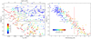 |
Fig. 1. Subsample of 246 Galactic O- and B-type stars investigated by Simón-Díaz et al. (2017), color-coded by the LC taken from Simbad. Left panel: location of the stars in a spectroscopic Hertzsprung-Russel diagram (see Sect. 3.1.1). The rough boundary between the O- and B-type star domains is indicated with the dotted diagonal black line. The evolutionary tracks taken from the MESA Isochrones & Stellar Tracks online tool for solar metallicity, and no initial rotation are included for reference purposes. Right panel: log(ℒ/ℒ⊙) against FW3414(Hβ) for the same stars. The vertical dashed red line and dashed horizontal black lines at log(ℒ/ℒ⊙) = 3.5 dex in both panels are included for reference (see Sect. 4.1). |
As mentioned in Sect. 1, we are interested in continuing the efforts initiated in previous papers of the IACOB series (referring to the O star domain; see Holgado et al. 2020, 2022), and populate with the largest possible sample, the region of the sHRD that corresponds to the B-type stars that are expected to be the descendants of the O-type stars. To this aim, one possibility would be to select the stars with spectral types in the range B0 to B9 from the initial sample described in Sect. 2.1 that are classified as supergiants (LC I) or bright giants (LC II). However, this approach requires caution because, as we show in Sect. 4.1, the spectral classifications provided by default by Simbad for the case of B-type stars include a non-negligible number of cases in which the LCs are incorrect (or not even provided). In addition, as illustrated in the left panel of Fig. 1, part of the region of interest is also populated by early-B giants (and maybe also subgiants and dwarfs). Therefore, if we follow this selection strategy, we might exclude many stars of interest for our study. To overcome this problem, we decided to follow a more robust (but still simple) strategy that is based on the use of the quantity FW3414(Hβ) as a proxy of the parameter log ℒ (both described in the next section).
3.1.2. Using the width of Hβ as a proxy of log(ℒ/ℒ⊙)
Considering the location of the O-type stars and the behavior of the evolutionary tracks in the sHRD shown in the left panel of Fig. 1, it might easily be assumed that at first glance, we are mainly interested in stars with log(ℒ/ℒ⊙) ≳ 3.5 dex, where the ℒ parameter is defined as  /g (Langer & Kudritzki 2014). Ideally speaking, the best approach for selecting our working sample of evolved descendants of O-type stars would be to have estimates of the effective temperature (Teff) and the surface gravity (log g) for each star in the list of potential targets of interest described in Sect. 2.1. However, although viable, this strategy would be very time-consuming because it would require the full quantitative spectroscopic analysis process for each target before the selection.
As an alternative, we decided to explore to which extent a direct measurement of the profile shape of one of the hydrogen Balmer lines, which are known to be affected by the surface gravity of the star through the effect of the Stark broadening, can be used to perform this selection in a much faster way.
In particular, we chose to work with the Hβ line, which is less affected by blends with other metal lines (as is, e.g., the case of the Hγ line) and is not as heavily affected by the presence of a stellar wind as the Hα line. As illustrated in Fig. 2 (see also the explanation below), we also identified that the quantity FW3414(Hβ), which is defined as the difference between the width of the Hβ line measured at three-quarters and one-quarter of the line depth, is better suited as a proxy of log(ℒ/ℒ⊙) than the full width at half maximum (FWHM) of the line.
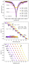 |
Fig. 2. Results from testing the method described in Sect. 3.1.2 measuring the FW3414(Hβ). Top panel: four illustrative Hβ profiles named A, B, C, and D for FASTWIND models with Teff = 24 000 K and R = 25 000, and different pairs of log g and v sin i. The horizontal pink lines indicate the position at three-quarters, one-half, and one-quarter of the line depth for example D. Middle and bottom panels: log(ℒ/ℒ⊙) against FW3414(Hβ) and FWHM, both measured in a grid of synthetic Hβ profiles from FASTWIND with the same Teff and R as in the top panel, and values of v sin i between 10 and 360 km s−1. The four profiles in the top panel are indicated with open circles and letters. The error bars in the middle panel show the average shift in all measurements due to the effect of different resolutions, and the effect of increasing Teff up to 30 000 K (approximate temperature for a B0 I–II star). |
To test the proposed method, we first used the stellar atmosphere code FASTWIND (Santolaya-Rey et al. 1997; Puls et al. 2005) to compute a grid of synthetic spectra corresponding to models covering a range in Teff = 16 000 − 28 000 K and log(ℒ/ℒ⊙) = 2.5–4.1 dex. The other parameters, such as the helium abundance (NHe), the microturbulence (ξ), and the wind-strength parameter (log Q)4, were kept fixed in the computation of the grid to NHe = 0.1, ξ = 10 km s−1, log Q = −14.0.
By convolving these spectra with different broadening and instrumental profiles, we were able to reproduce (to first order) the effect that different projected rotational velocities (v sin i) and spectral resolutions (R) have on the line profiles. In particular, we considered values of R between 2500 and 85 000, and eight values of v sin i, ranging from 10 to 400 km s−1. Some illustrative examples of the synthesized profiles are shown in the top panel of Fig. 2.
We then used the corresponding pyIACOB module to measure the full width of the line at three-quarters, one-half, and one-quarter of its depth for each simulated Hβ profile. For the same values of Teff = 24 000 K and R = 25 000, the middle and bottom panels of Fig. 2 show that for a given v sin i value, the lower the quantity log(ℒ/ℒ⊙) (i.e., the higher the surface gravity), the larger the quantities FW3414(Hβ) and FWHM. However, in a more general situation, the use of FW3414(Hβ) results in a more adequate proxy of log(ℒ/ℒ⊙) than the FWHM because it mitigates the effect that v sin i has on the shape of the line, providing a better indirect measurement of the gravity.
To better illustrate this situation, the top panel of Fig. 2 depicts four synthetic Hβ line profiles (named A, B, C, and D) that correspond to four different log g and v sin i combinations. Their location in the other two panels is indicated with open black circles and corresponding letters.
On the one hand, the aforementioned mitigation of the v sin i effect is clearly visible when the resulting differences obtained in FW3414(Hβ) (≲2 Å) and FWHM (≳6 Å) are compared when the profiles labeled A and B are considered. On the other hand, and more importantly, the FWHM produces a much less efficient filtering than the quantity FW3414(Hβ) when samples of stars with a broad range of v sin i are considered. For example, to ensure that a star with a set of parameters similar to those considered in profile B survives the filtering process, we need to assume a filtering value of FWHM ≈ 10 Å. Other stars with log(ℒ/ℒ⊙) down to ≈2.5 dex would also be selected in this case, however, which would contaminate the sample with many stars that are below the initially considered limit in log(ℒ/ℒ⊙) of ≈3.5 dex (see the left panel of Fig. 1). In contrast, since profile B has a FW3414(Hβ) ≈ 6.5 Å, considering this as the filtering value would only select stars down to log(ℒ/ℒ⊙) ≈ 3.5 dex, which corresponds to a star with similar parameters as those considered for profile C.
We note that the value of Teff = 24 000 K was not randomly chosen, but rather approximates the temperature of the majority of the B-type stars that we analyzed in this study (see Sect. 4.2.1). Similarly, the value of R = 25 000 was selected because the spectra used in this study have the same or a higher resolution. We have evaluated the effect of increasing Teff up to 30 000 K (approximate temperature for a B0 I–II star), which shifts our results by 0.5 Å toward higher values of the quantity FW3414(Hβ). Similarly, we investigated the effect of considering different resolving powers. We found that within the resolutions of our spectroscopic data set (see Sect. 2.1) the shift in FW3414(Hβ) is ≈0.2 Å toward lower values. On the other hand, we found an average shift of ≈0.2 Å compared to R = 5000 toward higher values, that is, ≈0.5 Å for R = 2500. In all cases, we obtained very similar slopes as those shown in the middle panel of Fig. 2, which demonstrates that the method can safely distinguish supergiants from low-luminosity counterparts in upcoming lower-resolution spectroscopic surveys such as WEAVE-SCIP (Dalton et al. 2020; Jin et al. 2023) or 4MIDABLE-LR (Chiappini et al. 2019).
As an additional validation of our proposed strategy, we measured the FW3414(Hβ) for all the stars included in the sHRD presented in the left panel of Fig. 1. We present the corresponding log(ℒ/ℒ⊙) vs. FW3414(Hβ) diagram in the right panel of Fig. 1, using the LC as the color code as in the left panel. Despite the very wide Teff span (more than 30 000 K) and different v sin i and resolutions, we are able to reproduce to a very good level what is shown in the middle panel of Fig. 2. These results allow us to provide an approximate value of log(ℒ/ℒ⊙) above which all stars very likely are descendants of the O-stars. In particular, if we wish to include all B-type stars with LCs I and II (BSGs), a value of log(ℒ/ℒ⊙) ≈ 3.5 dex can be used, and this would correspond to a FW3414(Hβ) of 7−8 Å.
3.2. Visual inspection of the spectra
The method described in Sect. 3.1.2 assumes a pure absorption profile for the Hβ line, but this is not always the case. Therefore, we decided to also perform a visual inspection of the spectra in order to identify cases in which the measurement of FW3414(Hβ) might be less reliable.
While inspecting the spectra, we did not only concentrate on the Hβ profiles, but also evaluated the global morphology of the Hα line. As a result, we were able to provide a rough classification of the different types of Hα and Hβ profiles that we found in the full sample. In addition, we benefited from the complete set of multi-epoch spectra that were available to perform a visual identification of the double-line or higher-order spectroscopic binaries (hereafter SB2+).
3.2.1. Identification of different Hα and Hβ profiles
Figure 3 shows some examples of the different types of Hα profiles we found in the spectra of the investigated sample of stars. These extend from pure absorption to strong emission (e.g., HD 54025 and HD 199478, respectively), cases in which the red wing is refilled (e.g., HD 15690), a P Cygni-type profile is detected (e.g., HD 206165 and HD 13256), or cases in which the profile appears contaminated by a more or less strong double-peak emission (e.g., HD 1544 and HD 23478). After a careful inspection of all the Hα profiles in our spectroscopic data set, we decided to establish a morphological classification that is based on five main different features (with some subtypes) as described below.
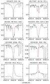 |
Fig. 3. Examples of different Hα profiles found within our sample. The name of the stars and spectral types and morphological labels (see Sect. 3.2.1) are included. The spectra are corrected for radial velocity by using a set of photospheric metal lines. The vertical dashed red lines indicate the reference position of the line. |
– Absorption (Ab): This classification applies when the line appears in pure absorption.
– Core filled (CF): This classification applies when the core of the line is filled with emission, but this emission does not pass the continuum level of the normalized flux. We set sublabels with CF, CF+, and CF++ to indicate when the central emission reaches approximately one-third, two-thirds, or up to the continuum level from the expected depth (see the top right panel of Fig. 3 for the last case).
– Double subpeak (DsP): This classification applies when both wings of the line are filled or are in emission above the normalized flux. This mainly accounts for fast-rotating stars with confined winds (see Petrenz & Puls 1996, Fig. 8 for more information). The labels DsP, DsP+, and DsP++ correspond to situations in which the filling of the lobes reaches one-third, two-thirds, or above the continuum of the line depth. The latter generally includes Be stars, in which both sides of the line are in strong emission due to the presence of a disk. Two cases for DsP+ and DsP++ (for a confirmed Be star) are included in the left and right second row of the panels in Fig. 3, respectively.
– Red filling (RF): This classification applies when only the red wing of the line is filled. The labels RF and RF+ separate situations in which the filling reaches one-half, or up to the continuum of the line depth, respectively. An example of an RF+ profile is shown in the left panel of the third row in Fig. 3.
– P-Cygni shape (PCy): This classification applies when the emission is in the red wing of the line profile. In the temperature domain of the stars in the sample, the shape is generally produced by stellar winds with specific characteristics (see, e.g., Castor & Lamers 1979). We use the sublabels PCy, PCy+, and PCy++ to indicate the observed the emission up to ≈1.25, between this and ≈1.5, and any value above ≈1.5 (traditional P-Cygni profiles) from the continuum, respectively. One example of the PCy and PCy++ shapes is included in the right panel of the third row and in the bottom left panel of Fig. 3, respectively.
– Pure emission (Em): This classification applies when there is emission above the normalized flux. Similarly to the P Cygni shape, we set the labels Em, Em+, and Em++ to indicate when the emission reaches up to ≈1.25, between ≈1.25 and ≈1.5, and any value above ≈1.5 from the continuum, respectively. The latter case is found in many Be stars. One example of an Em+ profile is included in the bottom right panel of Fig. 3.
This classification scheme was also applied to all Hβ profiles. Notably, there are many situations in which the labels assigned to both profiles are not necessarily the same (see Sect. 4.2.5). For example, in the case of classical Be stars with circumstellar disks, the Hβ profile may be labeled DsP+ or DsP++, while the Hα profile has Em+ or Em++. A similar situation may occur in the case of stars with strong winds, where the emission in Hα is expected to be more significant than in Hβ.
3.2.2. Identification of spectroscopic binaries
We also carried out a visual identification of SB2+ systems in the sample (see Sect. 3.2). To do this, we inspected the temporal behavior of several diagnostic lines (mainly He Iλ5875.62 Å, but also the Si IIIλλ4552.62,4567.84,4574.76 Å triplet, or other lines, e.g., Mg IIλ4481, C IIλ4267, or Si IIλ6371) using all the available multi-epoch spectra. Some examples of identified SB2+ systems can be found in Fig. C.1. We also refer to a forthcoming paper (Simón-Díaz et al., in prep.) that provides the detailed identification of the single-line spectroscopic binaries (SB1) using spectroscopic and photometric data.
3.3. Line-broadening analysis
Although the full quantitative spectroscopic analysis of the stars in the sample (see Sect. 4.2) will be presented in forthcoming papers, here we followed the guidelines in Simón-Díaz & Herrero (2014) and Simón-Díaz et al. (2017) to obtain estimates of the projected rotational velocities of all stars in our working sample. In brief, we used the IACOB-BROAD tool to perform a line-broadening analysis of a set of adequate diagnostic lines. In particular, for stars with v sin i ≲ 200 km s−1, we used a reduced set of unblended and strong absorption lines optimized for two ranges of spectral types. For stars earlier than B4, we used Si IIIλ4567.85 Å, except when the line was weak, in which case, we used Si IIIλ4552.622 Å. For B4 and later spectral types, we preferably used Si IIλ6371.37 Å, but depending on the spectrum, we also used Si IIλ6347.11 Å. However, the latter is blended with Mg II lines, and therefore, we only used it in a very few occasions. For stars with v sin i ≳ 200 km s−1, most of these lines are blended by other surrounding lines or became too diluted to provide reliable results. In this case, we decided to use He Iλλ4387.93,5015.68 Å lines, which are less affected by wind than other He lines and are well isolated.
4. Results and discussion
4.1. Sample selection
Figure 4 shows a histogram with the results of the FW3414(Hβ) measurements for the complete initial sample of stars described in Sect 2.1. We point out here that the fitting of the Hβ failed in ≈100 stars. About ≈75% of these correspond to Be stars, ≈15% correspond to SB2+ stars, and ≈10% correspond to hypergiants. The histogram separates different groups according to the LC quoted by default in Simbad and includes two additional groups that comprise on the one hand, the stars for which Simbad does not provide any LC (pink), and, on the other hand, the stars that we identified as SB2+ (gray; see Sect. 3.2.2).
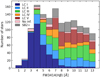 |
Fig. 4. Histogram of the number of stars in bins of FW3414(Hβ) for the initial sample of O9 – B9 type stars. In each bin, the number of stars is stacked by luminosity class with different colors. The spectral classifications have been taken from Simbad. The sources without a luminosity class are grouped in pink under the label “No inf.”. Independent of their LC, all stars classified as SB2+ are grouped in bins in gray. |
The measured FW3414(Hβ) for the LC I stars peaks at ≈4 Å, and, except for a few cases, this LC group extends to FW3414(Hβ) ≈ 7.5 Å. Instead, stars with LC II, III, and IV are present in a wider range, with FW3414(Hβ) ≳ 4 Å, while stars with LC V are mostly concentrated at FW3414(Hβ) ≳ 6.5 Å.
Figure 5 helps us to better understand the distribution of the various luminosity class groups in this histogram. Similarly to Fig. 1, the left panel of this figure shows an sHRD, while the corresponding log(ℒ/ℒ⊙)–FW3414(Hβ) diagram is shown in the right panel. This time, both diagrams are populated with a much larger sample, resulting from the preliminary quantitative spectroscopic analysis of a subsample of the stars we used to build Fig. 4, and comprising ≈500 O9 – B6 type stars. Figure 1 includes 9 SB2+ systems in which the effect of the secondary in the spectrum was such that it allowed for determination of some rough spectroscopic parameters. In addition, stars for which Simbad does not provide a luminosity class are represented as pink circles. The sHRD includes an additional sample (gray circles) of 280 likely single and SB1 stars investigated by Holgado et al. (2020).
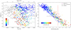 |
Fig. 5. Preliminary results from the quantitative spectroscopic analysis of ≈500 O9–B6 type stars presented in this work for which the FW3414(Hβ) has been measured. The color code in both panels indicates the LC taken from Simbad. Left panel: sHRD for these stars and additional results from Holgado et al. (2018), indicated with gray dots. The evolutionary tracks are taken from the MESA Isochrones & Stellar Tracks online tool for solar metallicity and no initial rotation. The approximate separation between O- and B-type stars is indicated with the dotted diagonal black line. The dashed horizontal black line at log(ℒ/ℒ⊙) = 3.5 dex used in the selection of the working sample is indicated (also shown in the right panel). Right panel: log(ℒ/ℒ⊙) against FW3414(Hβ) for the same ≈500 stars. The vertical dashed red line shows the value we adopted to select the working sample. Open circles indicate stars with v sin i > 120 km s−1, and gray crosses are SB2+ systems. Stars without luminosity classes in Simbad are plotted in pink. |
First of all, by comparing the middle panel of Fig. 2 and the right panel of Fig. 5, we can confirm the good agreement of the model predictions and empirical measurements. Interestingly, fast-rotating stars tend to be located to the right of the rest of stars for each luminosity class, as predicted. Last, we note that the location of the stars that are identified as SB2+ in the log(ℒ/ℒ⊙)–FW3414(Hβ) diagram is not particularly different from the rest of the stars with similar LC. This therefore indicates that the contribution of the two stellar components does not strongly affect the FW3414(Hβ) estimate, at least when one of the two components dominates the spectrum.
The location of the stars in the left panel of Fig. 5 shows that most of the stars with LC I have log(ℒ/ℒ⊙) ≈ 3.8–4.3 dex. The right panel of the same figure shows that this range in log(ℒ/ℒ⊙) implies a range in FW3414(Hβ) ≈ 1.8–6 Å, which explains the distribution of LC I stars in Fig. 4. For lower values of log(ℒ/ℒ⊙), the situation is more mixed. For example, the stars in the log(ℒ/ℒ⊙) ≈ 3.5–3.8 dex range have LCs V–IV at Teff > 30 000 K, but also II–I at Teff < 20 000 K. Essentially, all stars except for those with LC I lie between log(ℒ/ℒ⊙) ≈ 2.8 and 4.2 dex, which also explains their wider distribution in Fig. 4.
We also conclude based on the two panels of Fig. 5 that some of the classifications taken from Simbad may not be correct. For instance, they were especially suspicious for stars with LC I and some II with log(ℒ/ℒ⊙) < 3.5 dex that are embedded in the sHRD, where stars with LCs III–IV–V lie. To confirm this situation, we reviewed the spectral classifications of many of these stars using our own available spectra or alternatively, previous classifications that in our judgment come from reliable references. The outcome of this exercise is summarized in Table D.1. As expected, most of them are early B-type stars that should be classified as giants, subgiants, or dwarfs. We also found that in many cases, we can attribute misclassifications to the fact that they were made using spectra at low resolution, as is the case of many classifications from Houk & Swift (1999) at R ≲ 2500.
This result again highlights the risk of using spectral classifications (especially if they come from heterogeneous sources) to select specific groups of stars and makes our proposed strategy much more robust and reliable. Moreover, this strategy has also allowed us to recover a non-negligible number of adequate candidates of interest among the stars quoted as OB or O stars in Simbad, or for which luminosity classes are not provided in Simbad that we would otherwise have missed. Revised spectral classification for these stars, following the guidelines indicated above, are provided in Tables D.1 and D.2.
As mentioned in Sect. 3.1.2, a good threshold value to select the evolved descendants of O-type stars is at log(ℒ/ℒ⊙) = 3.5 dex. Based on the empirical correlation between log(ℒ/ℒ⊙) and FW3414(Hβ) shown in the right panel of Fig. 5, we decided to use a filtering value of FW3414(Hβ) = 7.5 Å to select our sample (see below), which comprises a total of 728 stars.
By choosing this value, our selection criteria first became very effective in the selection of stars with LCs I – II, especially now that we have confirmed that almost all stars with log(ℒ/ℒ⊙) < 3.5 dex quoted in Simbad as LC I and II are LCs III, IV or V objects. In addition, as already pointed out in Sect. 3.1.1, our method also selects a significant number of stars with LCs III-IV-V (mostly early B giants and subgiants), which are of interest for the purposes of our study, which aims to perform an empirical characterization of the B-type stars that evolve from the MS O-type stars.
Due to the scatter of the log(ℒ/ℒ⊙) – FW3414(Hβ) correlation, we selected some stars with log(ℒ/ℒ⊙) in the range 3.1–3.5 dex (see right panel of Fig. 5), however. This inherent limitation of the proposed method does now allow us to exclude them without first determining their Teff and log(ℒ/ℒ⊙), or at least using additional information such as photometric data to filter these stars (see Sect. 4.2.2).
To conclude this section about the selection process, we now define our final (working) sample as the stars that are selected with the above-mentioned strategy, plus some additional hypergiant stars identified from the initial sample based on their characteristic P-Cygni profiles in the Hβ line (Lennon et al. 1992), leading to a final number of 733 stars. Although we were unable to obtain a reliable FW3414(Hβ) measurement for all the hypergiants, they are, in principle, also natural descendants from the O-stars. All of them (12) are listed in Appendix F. All the other stars without FW3414(Hβ) are considered for the completeness of the sample (see Sect. 4.2.3), as also in the forthcoming paper dedicated to spectroscopic binaries in the case of the SB2+ systems, but they are all excluded in the following sections.
4.2. Sample description
Table H.1 gathers the relevant information for the 733 stars resulting from the selection process described in Sect. 4.1. It includes an identifier of the star (ID), its B magnitude, and spectral classification (following Simbad); the name of the fits-file in the format of the IACOB spectroscopic database corresponding to the best spectrum (see Sect. 2.1) and its characteristic S/N in the 4000−5000 Å region; the measured value of FW3414(Hβ), whether the star has been identified as a spectroscopic binary (see Sect. 4.2.4); the morphological classification of the Hα and Hβ lines (see Sect. 4.2.5) and, last, the estimated v sin i (see Sect. 3.3). Although in Table H.1 we quote the spectral classifications provided by default by Simbad, we already pointed out that some of these classifications are inaccurate or even incorrect in some cases. The SpT and LC of stars whose spectral classifications we reviewed (see Sect. 4.1) are listed in parentheses. For the rest of this section and subsections, we adopted all the new classifications included in Appendix D to better interpret the results from the selection method.
In addition, for all the above-mentioned stars, Tables H.2 and H.3 gather most of the relevant photometric and astrometric information from Gaia or HIPPARCOS, respectively. The two tables include the same identifier of the star as in Table H.1, the Galactic coordinates (l, b), the parallax (ϖ) and proper motions (μα cos δ, μδ), and the distance, which in the first case was retrieved from Bailer-Jones et al. (2021; Distance B − J), and in the second case from the inverse of the parallax as a rough estimate (Distance). Table H.2 additionally includes the Gaia G, GBP, and GRP band magnitudes and the RUWE value, while Table H.3 includes the B − V magnitude. In some cases when the available data had very large errors, negative parallaxes, or any other issue, we did not include the distance. These cases usually match with bright targets.
4.2.1. Spectral types and luminosity classes
Figure 6 shows a histogram summarizing the spectral classifications of the stars in the final sample. As expected from the selection criteria (see Sect. 4.1), the majority of the sample consists of supergiants (364) and bright giants (119) compared to stars of other classes. In particular, it shows that while stars between O9 and B1 cover all luminosity classes, from B2 and especially B3 onward, the relative number of giants and especially subgiants and dwarfs decreases noticeably. From B4 and toward later-type stars, practically all our sources are classified as supergiants. Interestingly, despite the large number of stars included in our investigated sample, there is a clear lack of stars that are classified as B4 supergiants and bright giants.
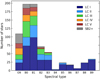 |
Fig. 6. Histogram of the number of stars in bins of spectral types for the final sample of stars. In each bin, the number of stars is stacked by luminosity class with different colors. Independent of their LC, all stars classified as SB2+ are stacked in gray bins. |
4.2.2. Astrometry and photometry
Figure 7 shows a stacked histogram of the adopted distances for all the stars up to 4000 pc. Fifty percent of the stars have distances derived from HIPPARCOS. They were excluded because their values of σϖ/ϖ ≥ 0.1 (see also Table H.3). This histogram is complemented by Fig. 8, which shows the distribution of the stars in a polar plot using Galactic coordinates, and centered at the position of the Sun.
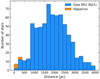 |
Fig. 7. Stacked histogram of the number of stars in bins of 200 pc for the final sample of stars up to 4000 pc. The distances were obtained either from Bailer-Jones et al. (2021; blue bins) or using the inverse of the parallax from HIPPARCOS for stars without Gaia DR3 data (orange bins). The latter are limited to those with σϖ/ϖ ≤ 0.1. |
Below 700−800 pc, the total number of stars is relatively low (≲50). These stars are considered to form the Gould Belt system (Poppel 1997), but recent studies suggested that this structure is in fact not real (see, e.g., Bouy & Alves 2015; Zari et al. 2018). Then, the number of stars suddenly increases with distance, as is expected from the volume increase, but it also increases due to the inclusion of several large clusters and association of massive stars such as Cep OB2 (l ≈ 100°, d ≈ 900 pc; Contreras et al. 2002), Sgr OB1 (l ≈ 5°, d ≲ 1400 pc; Melnik & Dambis 2020), Sco OB1 (l ≈ 340°, d ≈ 1600 pc; Damiani et al. 2016; Yalyalieva et al. 2020), or Cyg OB2 (l ≈ 80°, d ≲ 1700 pc; Berlanas et al. 2019; Massey & Thompson 1991), many of which are embedded in the Sagittarius arm or in the newly discovered Cepheus spur (Pantaleoni González et al. 2021).
The number of stars at 1000−2400 pc remains more or less constant up to ≈2500 pc, when it begins to decrease significantly. The number of stars is expected to increase significantly with increased volume after 1000 pc, but we do not observe this. While one possible and simple explanation might be observational biases (discussed in Sect. 4.2.3), this can also be caused by the lack of structures with young formed regions. This has been observed from distances above 3000 pc, where we also observe a drop. However, at these distances, the stars begin to be too faint to be observed using the facilities that were used to build this sample (see below).
Figure 8 shows that in general, there are no regions with average higher errors than others, but only some dispersed stars in the plane and likely with incorrect distances. In addition to the above-mentioned associations and galactic structures, the location of many others extend up to 3 kpc, such as the Per OB1 association (l ≈ 130°, d ≈ 2400 ± 200 pc; Garmany & Stencel 1992; de Burgos et al. 2020; Melnik & Dambis 2020) or the Car OB1 (l ≈ 300°, d ≈ 2300 pc; Shull et al. 2021). This result tells us about the fact that our sample is concentrated in relative close groups in the Galaxy following star-forming episodes, similarly to what was found by Pantaleoni González et al. (2021, Fig. 5). Additionally, there are large empty areas with a very low density of stars (many of which are likely runaways from the main clusters). While some of the empty areas can be attributed to gaps between the spiral arms in which no star formation occurs, others can be attributed to very high extinction (e.g., toward the direction of l ≈ 45°), the latter especially in the direction of the Galactic center (see Lallement et al. 2018, 2019).
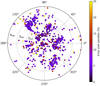 |
Fig. 8. Polar plot in Galactic coordinates of the stars in the final sample, centered at the position of the Sun and up to a distance of 4 kpc. The stars are colored by the σϖ/ϖ parameter between 0% and 25%. Stars with distances taken from HIPPARCOS are limited to those with σϖ/ϖ ≤ 0.1. |
Last, Fig. 9 shows the stars in the sample in a histogram of the apparent Bmag magnitude. The stars with distances taken from HIPPARCOS are all located within the first 100 pc in Fig. 7. The fact that most of these stars are among the brightest ones is not casual, as Gaia is known to have saturation issues for the brightest targets (see Lindegren et al. 2018), thus missing the astrometric and photometric data. This histogram also shows that the number of stars exponentially increases up to Bmag ≈ 9.5 and then decreases rapidly. This is expected because fainter stars become less suitable for an adequate use of the considered observing facilities (see Sect. 2.1), in order to reach a balance between the exposure times and S/N.
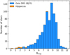 |
Fig. 9. Histogram of the number stars in the sample with the Bmag magnitude for the stars in the sample in bins of 0.5 mag. Stars with distances taken from HIPPARCOS with σϖ/ϖ ≤ 0.1 are indicated in orange. |
Figure 10 provides a different and complementary view of the sample, this time in a color-magnitude diagram (CMD) constructed using data from Gaia DR3. Similarly to the case of Fig. 5, a gradient in the position of the stars with LC from I-II down to III–IV–V is visible. More interestingly, compared to the expected location of the investigated sample of stars in the CMD (if they were not affected by extinction), namely, between the depicted 9 M⊙ and 40 M⊙ evolutionary tracks, almost no stars populate this region. This indicates that an important fraction of stars in our sample is expected to be affected by extinction higher than 1 mag (and up to 3−4 mags in some cases). This diagram is inefficient for a classification into O- and B-type stars beyond providing a rough estimate of the luminosity class: the range of variation in GBP − GRP of the evolutionary tracks is negligible compared to the scatter of the empirical sample due to the extinction. More specifically, we accounted for ≈50 O9 – B1 LC I stars with GBP − GRP > 0.80, that is, with a very high reddening compared to the reddening of the same type that is present at GBP − GRP ≈ 0.0.
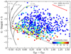 |
Fig. 10. Gaia DR3 Gmag corrected for distance against GBP − GRP for the selected sample, color-coded with the LC. The solid black line shows the ZAMS. The evolutionary tracks for 9, 15, 20, and 40 M⊙ up to the end of the He-burning phase obtained from MESA without initial rotation or extinction are shown in gray. No reddening is applied. Instead, a reddening vector with Δ(Av) = 1 is indicated with the red arrow. Two diagonal dashed black lines show two extinction lines for a 20 M⊙ star and for the approximate position in Fig. 5 in which the same track crosses the value of log(ℒ/ℒ⊙) ≈ 3.5 dex, respectively. |
The top extinction line in Fig. 10 was chosen to locate the approximate position of the stars that evolve from the O-type and contain all the BSGs because it coincides with the approximate separation between O- and B-type stars. Although this approach might also be used together with FW3414(Hβ) to filter undesired stars, we decided not to use it because of the large uncertainties in the distance of some of the stars in the sample (especially for the bright targets). While some stars are incorrectly classified with LC I (Sect. 4.1) some others are likely below this top extinction line due to underestimated distances. The latter is compatible with the scenario presented in Pantaleoni González et al. (2021), who used a different prior that produced longer distances compared to those used in this work from Bailer-Jones et al. (2021). Nevertheless, most of the stars in the sample are located above the top extinction line.
We recall here that our selection method based on the values of FW3414(Hβ) also selects stars with 3.5 ≳ log(ℒ/ℒ⊙)≳3.1 dex. Despite the possibility of underestimated distances, most of these stars are located between the two reddening lines, which indicates that by using the correct distances, this method effectively selects stars.
4.2.3. Completeness and observational biases
This section is dedicated to providing an overview of the completeness and potential observational biases that affect our sample. As shown in Fig. 9, this sample was mostly built to be a magnitude-limited sample. In this regard, it is important to remark that any use of this sample to empirically constrain evolutionary models, for instance, must take into account that for a given limiting magnitude, there will be more mid to late B-type stars than early B- or O-type because the first are intrinsically brighter in this band than the latter group, and are therefore observable at larger distances (ignoring extinction). However, as shown in Sect. 4.2.2, many stars within the sample have very different reddening, which dims their brightness up to several magnitudes. As a consequence, the extinction must be taken into account to unbias the sample from potentially fainter stars that are in fact at closer distances. To overcome these biases, one possibility is to investigate to which extent we can build a volume-limited sample (see below).
In order to assess the completeness of our sample within a specific volume or distance, we cross-matched our database with the ALS III catalog (Pantaleoni González et al., in prep.), which not only includes all the stars in our sample, but also provides an increased number of stars compared to earlier releases by including fainter objects (down to Bmag ≈ 16) and covering a larger distance (up to 10 000 pc). However, despite the authors’ claim of high completeness within the first 5000 pc, the fraction of stars with Bmag > 16 within this distance is not negligible due to extinction along the line of sight. For instance, if we consider stars up to 2000 pc and use the absolute V-band magnitudes from Lesh (1968), the intrinsic faintest stars within our sample could have a maximum extinction of Av = 8−9 in order to have Bmag ≤ 16 (see further notes in Appendix E). While some star-forming regions within this distance exhibit average extinction values close to this limit (e.g., Cyg-OB2, Av = 5−7; Massey & Thompson 1991), highly obscured massive stars have been found to have extinctions exceeding this limit (see, e.g., Callingham et al. 2020), thus indicating that a complete sample cannot be assumed. Nevertheless, we consider the ALS III to be a very good reference to find missing stars within the observing magnitude limitations.
Figure 11 presents a similar CMD diagram as we showed in Fig. 10, but this time, including all stars quoted in the ALS III catalog that fulfill the following criteria: (1) they are classified as O9 – B9 in Simbad, (2) they are located above the extinction line corresponding to a ZAMS star of 9 M⊙, (3) they have a Bmag < 11, and (4) their estimated distance, derived as described in Sect. 2.2 for the case of our working sample, is below 4000 pc. We are mostly interested in the stars located above log(ℒ/ℒ⊙) = 3.5 dex, which correspond to the sample located above the top reddening line (green stars). We therefore only discuss the completeness and potential observational biases that affect this region. Before we discuss this, we remark that even considering the full sample of O9 – B9 stars in ALS III, the lack of stars in the region of the diagram in between the non-reddened 15−40 M⊙ evolutionary tracks still persists.
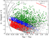 |
Fig. 11. Same as Fig. 10, but now including O9 to B9 stars from the ALS III catalog (Pantaleoni González et al., in prep.) limited to stars Bmag < 11, and distances of 4000 pc. The two diagonal dashed black lines mark the reddening line of a 20 M⊙ star. They establish three regions in the diagram that are expected to be mostly correlated with log(ℒ/ℒ⊙), as described in Sect. 4.2.2. The bottom line starts from the ZAMS, and the top line starts from the approximate age at which it intersects the horizontal dashed black line in the left panel of Fig. 5 at log(ℒ/ℒ⊙) = 3.5 dex. Both extended up to a Δ(Av) = 2. The stars in the full sample of observed O9–B9 type stars for which the upper and lower distances based on the errors lie above the top reddening line are shown in green, those for which one of the distances lies between the two reddening lines are shown in blue, and those for which one of the distances lies below the bottom reddening line are shown in red. The remaining stars populating the CMD are plotted in gray and correspond to stars that are not yet observed. Four tracks from MESA with Av = 0.0 and no initial rotation are included for 9 M⊙, 15 M⊙, 20 M⊙, and 40 M⊙. |
To visually evaluate the completeness, Fig. 12 shows a stacked histogram of the selected sample of stars from ALS III that are located above the top reddening line of Fig. 11, indicating the stars for which we have spectra, and separating the missing stars into those with Bmag < 9, and those with 9 < Bmag < 11. In addition, we highlight the stars with a GBP − GRP > 0.5, that is, we indicate the targets that are more strongly affected by extinction.
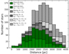 |
Fig. 12. Histogram summarizing the completeness of the sample respect to the ALS III catalog for stars above the top reddening line of Fig. 11 (see Sect. 4.2.3 for more details), in bins of 250 pc of distance. Observed O9 – B9 stars are in green, while missing stars from the ALS III are colored in two gray colors: in dark gray, missing stars with Bmag < 9, and in light gray, stars with 9 < Bmag < 11. For each group, hatched areas indicate those stars with GBP − GRP > 0.5. |
This figure is complemented by the information provided in Table 1, were we present a summary of the total number of stars and relative completeness of stars in the above-mentioned region of the Gaia-CMD for four different distance ranges, and we separate stars below or above the Bmag = 9 threshold. The corresponding statistics are given for the complete sample as well as for the stars that can be observed from the northern hemisphere (i.e., with δ > −20° using either the NOT or Mercator telescopes).
Summary of the completeness of the sample for four different distance ranges.
Up to 2000 pc, the sample is complete up to 77% of the total stars with Bmag < 9. This number is reduced to 58% for the stars that are located farther away. It is important to point out that the IACOB project observes only with the NOT and Mercator telescopes from the northern hemisphere (see Sect. 2.1). In the case of the southern hemisphere, we are currently limited to FEROS objects retrieved from the ESO public archive. In fact, only 20% of the spectra come from FEROS. To state this in numbers, if we only consider the stars with declination above −20°, we currently miss 30% from those up to 2000 pc (93 stars) with Bmag < 11, and only 13% (44 stars) with Bmag < 9 up to 4000 pc. These missing (northern) stars are currently in observing queues for upcoming IACOB observing campaigns. Regarding the missing sources with declination below −20° up to 4000 pc (162 stars with Bmag < 9, and 321 with 9 < Bmag < 11), we are currently in the process of improving the situation through a recently approved proposal. In particular, the awarded time is ≈250 h distributed in two semesters. with FEROS. Last, we evaluated the contamination of classical Be stars in the completeness because these stars are not of interest here. We concluded that while they only represent ≈11% of all the stars in Fig. 12, they are homogeneously distributed in Fig. 11 above the top reddening line (but close to it), and therefore, they do not affect the results in Table 1.
Figure 13 provides a complementary view of the available and missing stars, this time showing their location in the Galaxy and following the same color code as in previous figures, but separating the stars by their GBP − GRP value in two groups. Globally, for the region between l = 0° and 230°, the completeness is very high, while the missing southern stars are located between 230° and 0°. The top panel for stars with GBP − GRP < 0.5 shows the less reddened stars. The reason for separating stars with −20° in Table 1 is also more evident: The vast majority of the missing stars are concentrated in the Carina region of the southern hemisphere (l ≈ 270° −315°, d ≈ 2500 pc). Additionally, most of the missing stars in this panel have Bmag < 9 (dark gray circles), while almost no stars with 9 < Bmag < 11 (light gray circles) are located within 2000 pc. The bottom panel instead shows the more reddened stars, most of the missing stars of which have Bmag > 9. They are located not only in the Carina region, but also in some other specific regions such as the Sagittarius region (l ≈ 340° −25°, d ≈ 1000 − 2500 pc), the Cygnus region (l ≈ 80°, d ≈ 2000 pc), and the Cassiopeia region (l ≈ 115° −135°, d ≈ 2500 − 3500 pc). The fact that many stars are observed in some of these regions shows the very different existing degrees of extinction (see, e.g., the Cygnus region). Interestingly, most of the missing stars in the northern hemisphere are spread throughout a wide space in the Cassiopeia region.
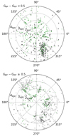 |
Fig. 13. Two polar plots in Galactic coordinates of all the stars above the top reddening line of Fig. 11, separating in the top and bottom panels those with GBP − GRP ≶ 0.5. In both panels, light gray or gray circles indicate missing stars separating those with 9 < Bmag < 11 or Bmag < 9, respectively, and with green circles the stars for which spectroscopic data are available. |
Regarding the observational biases within the spectral classifications, we carried out homogeneous observations in the northern hemisphere trying to ensure completeness within the B0–B3 I-III and B3 – B9 I-II type stars up to Bmag = 9. In fact, the percentages given in Table 1 increase by 5% to 10% when only the stars of LCs I and II are considered. Of the stars with LCs III–IV–V, ≈80% are already observed, and we expect this percentage to reach ≈95% in the next upcoming campaigns, taking into account that in this case, a non-negligible number will be Be stars, which not of interest here.
To summarize, we can confidently say that we have achieved a homogeneous and unbiased sample with a high degree of completeness with respect to the ALS III catalog, except for stars with δ ≲ −20 deg, and this also shows the success of the IACOB project within the past ten years of observing in the northern hemisphere.
4.2.4. Identification of double-line spectroscopic binaries
As explained in Sect. 3.2.2, we also visually inspected all the multi-epoch spectra in our serach for potential SB2+ systems. Figure 4 shows that the fraction of SB2 systems is smaller toward higher FW3414(Hβ) values, and there are almost none such systems below 4.5 Å. Within the stars that fit the selection criteria (see Fig. 6), we account for 56 SB2+ systems, and it is unclear for additional 7 systems whether they are SB2 systems or if the features in the diagnostic lines are caused by long profile variability. These systems are indicated as LPV/SB2? in the SB column of Table H.1 and will require additional spectroscopic observations and possibly photometric analyses to determine whether they are binary systems or if the features observed in the spectra correspond to variability, such as pulsations. Fife of the 56 SB2+ systems have a third component (formally SB3 systems). Twenty-one systems correspond to B-type stars and the rest are O9-type stars. We identified 8 new systems. The new identifications are marked with an asterisk in the SB column. Some of the cases (HD 7252, HD 12150, and HD 46484) were already proposed as multiple systems based on the astrometric anomalies (Kervella et al. 2019), or they were photometrically observed as eclipsing binaries (HD 142634, HD 153140, and HD 170159).
Figure 6 also shows that compared to the number of binary systems with an O9-type primary star, the number of systems with a B-type primary within the sample is much lower. Although several studies have estimated multiplicity for O-type stars (e.g., Barbá et al. 2010; Sana et al. 2013), not as many have explored the B-type domain, and most of them only covered the dwarf star regime, with many classical Be stars within their samples (e.g., Evans et al. 2006; Bodensteiner et al. 2021; Banyard et al. 2022). The number of studies dedicated to cover the B-type supergiants is even smaller (Dunstall et al. 2015; McEvoy et al. 2015). We have found that the fraction of O9-type binaries in the sample is 23% and there are 3.6% B0 – B9 stars in the sample (i.e., mostly including I–II type stars), which is about six times less. This observed decrease is expected from the natural evolution of these objects because some of them may either have become much more luminous than the companion (by evolution or mass transfer; Langer 2012; de Mink et al. 2013), merged into a single more massive object (e.g., Podsiadlowski et al. 1992; Vanbeveren et al. 2013), or were even separated after supernova (e.g., de Mink et al. 2011, 2014), and only the less evolved companion remained.
4.2.5. Morphology of the Hβ and Hα profiles
Figure 14 shows four histograms indicating the number of stars as a function of SpT and LC for which the various types of Hβ and Hα profiles presented in Sect. 3.2.1 are identified. We note that because the stars labeled CF, DsP, PCy, and RF still have a strong absorption shape, they were joined with the stars labeled Ab (Absorption) for the purposes of this figure. We also removed all the SB2+ systems here.
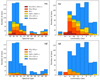 |
Fig. 14. Results of the number of stars against their spectral type (two leftmost panels) and luminosity class (two rightmost panels), represented in histograms. Each bin stacks the number of stars with different morphologies found for the Hβ and Hα profiles following the classification in Sect. 3.2.1 and grouped as in the legend. Stars labeled within the “Absorption” label include profiles CF, DsP, PCy, and RF. The sources with LC I without subtype in the literature are grouped into a separate bin. The sources classified as SB2+ are removed from the bins. |
As illustrated in the bottom two panels of Fig. 14, the majority of the stars have Hβ profiles in absorption, with the exception of a group of stars labeled RF+ (red wing filled) and PCy/PCy+ (P-Cygni shape), both evidencing the presence of winds (Lucy & Solomon 1970; Castor et al. 1975). This group is concentrated within SpT O9 – B2 and LC I (and subtypes). Most of those labeled PCy+ correspond to hypergiants (Ia+), as shown in the bottom right panel (see also Appendix F).
The two panels at the top show a more mixed situation for the Hα line. This is because the effect of the stellar winds on the Hα profile is stronger than on the other hydrogen lines of the Balmer series. Interestingly, the relative fraction of stars with Hα in absorption with respect to the total for each bin decreases toward later spectral types (it is ≈50% on average). A similar decrease occurs in the luminosity classes from dwarf stars toward the supergiants. In particular, most of the stars with LCs Ia+, Ia, Iab are labeled RF+ and PCy/PCy+, which is also the case of the B8–B9 type stars. The extended presence of P Cygni shapes is expected because it is well known that B-type supergiants have stronger stellar winds than other less luminous stars (Kudritzki et al. 1999; Markova & Puls 2008). Stars with Hα in emission (7% of the total) are present in all spectral types, but are mostly concentrated in LC I. In fact, nearly 90% of the stars with LCs IV and V have absorption profiles in Hα. This indicates that stars affected by winds are located at higher luminosities. Last, profiles with sub-double-peak emission make up 10% of the total, and those in which the core of the lines is filled make up only 2%.
4.3. First hints about the rotational properties of the sample
The top panel of Fig. 15 shows a histogram of the projected rotational velocities of our working sample (excluding the stars labeled SB2+ and some problematic cases), highlighting in different colors the different LCs of the stars, and including seven stars with v sin i > 340 km s−1 in the last bin. This distribution has a mean and median values of 80 km s−1 and 51 km s−1, respectively (64 km s−1 and 47 km s−1 for stars with LCs I and II), and a standard deviation of 74 km s−1 (50 km s−1), with ≈85% of the sample having values below 150 km s−1, which is followed by a tail of fast-rotating stars. In addition, the bottom panel of the same figure shows the corresponding cumulative distribution. There, stars with brighter luminosity classes reach higher fractions earlier than those that are less luminous. In particular, for the supergiant stars they reach 80% within the first 70 km s−1 alone. The rest increase more or less gradually.
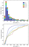 |
Fig. 15. Histogram and cumulative distribution of the v sin i in the sample stars, excluding the identified SB2+ stars. In the top panel, each bin of the histogram is 20 km s−1 wide and stacks the stars separated and color-coded by their LC. In the bottom panel, we plot the cumulative distributions separated by LCs. |
Stars with LCs I and II, which are the main drivers of our study, are shown in the main plot of Fig. 16. For each SpT in the O9 – B9 range, the median of the v sin i distribution and upper and lower limits corresponding to percentiles 90%, 75%, 25%, and 10% are plotted. The main characteristic of the figure is that the mean values for both LCs gradually decrease down to 30 km s−1 for the B3-type stars and remain in that value up to the B9-type stars. This behavior also holds at the lower limits of the error bars (slowly rotating stars). The second main characteristic is that the upper limits of the percentiles (mainly corresponding to the faster-rotating stars) also follow the same trend up to the B3-type, where their number suddenly drops. In more detail, the panel inside includes histograms of the v sin i distribution for the B1-type stars separating LCs I from II, illustrating the above-mentioned characteristic. There, the main distribution is centered at ≈50 km s−1, followed by a relatively smooth tail of these fast-rotating objects, with v sin i extending up to 300 km s−1.
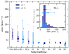 |
Fig. 16. Main panel: distribution of the median of v sin i obtained through the GoF method of IACOB-BROAD against the SpT, separated into stars with LCs I and II. The solid error bars indicate the upper and lower limits corresponding to the 75% and 25% percentiles, and the dashed error bars correspond to 90% and 10% percentiles. Stars without LC or SB2+ systems are not included. Small panel: histogram of the subsample of B1 I–II stars against the v sin i for a better interpretation of the main paneland Sect. 4.3. The error bars corresponding to the B1 I–II stars are plotted horizontally. |
To compare our results with some other results of v sin i from the literature, we mainly considered studies that also used large samples of O-stars and BSGs. For instance, Howarth et al. (1997) obtained a median value of 91 km s−1 for 373 stars, with an average difference between O- and B-type of 25 km s−1, that is, higher for O types. Compared to our results, the slightly higher values obtained there can be explained when the effect of macroturbulence broadening is taken into account, which can shift v sin i by ≈25 km s−1 (Simón-Díaz & Herrero 2014). This is shown in Fraser et al. (2010), who found a ≈30 km s−1 offset with the stars in common with Howarth et al. (1997) from their sample of 57 Galactic BSGs. These authors obtained mean values of ≈60 km s−1 with a standard deviation of 50 km s−1, which is very similar to our results (see also Hunter et al. 2008; Simón-Díaz & Herrero 2014, for more examples including BSGs).
Similarly to Fig. 16, Fraser et al. (2010) and Simón-Díaz & Herrero (2014) included distributions of v sin i with respect to the SpT for stars with LCs I and II, although the latter only reached B2-type stars. In both cases, their results are very similar to ours. On the one hand, in all the cases v sin i values decrease toward mid-B-type stars. However, our significantly larger sample (comprising seven to eight times more stars) clearly extends the presence of fast-rotating stars with v sin i ≥ 100 km s−1 up to the B3-type stars. On the other hand, the slow decrease given by the mean values might be explained by the natural evolution of the stars, decreasing their v sin i as they increase their radii. However, this decrease does not continue after the B4-type stars, suggesting that either they loose enough angular momentum during their evolution (e.g., via stellar winds; Vink et al. 2010) or that our methodology does not allow us to measure the actual v sin i below a certain threshold limit (see Simón-Díaz et al. 2017).
We also compared our results for the v sin i with those from Holgado et al. (2022) for the O-type stars (see the gray dots in Fig. 5) to show the differences with the BSGs as the first are the progenitors of the second. A simple comparison with Fig. 15 indicates a similar distribution that includes a main group of stars at lower v sin i values, followed by a tail of fast-rotating stars. Moreover, the stars with LC I are concentrated at v sin i ≲ 150 km s−1, similarly to our sample of stars of the same LC. Moreover, the cumulative distributions for this LC also look very similar. Last, the results from Holgado et al. (2022) for stars located between the 20−32 M⊙ evolutionary tracks (i.e., those evolving into the early B-type III–IV–V stars) also show higher v sin i values than those directly above, which is the same situation as we showed in Fig. 15, even though our sample is biased by the relative number of stars with LCs III–IV–V with respect to I and II.
These results clearly indicate that the v sin i values do not significantly decrease during the transition from O-type stars toward the BSGs (and the additional B-type III–IV–V stars), thus favoring evolutionary models in which the braking effect is weaker and/or the angular momentum transfer from the cores to the outer layers is very efficient and counteracts the effect (see Brott et al. 2011).
5. Summary, conclusions, and future work
We have built a homogeneous spectroscopic sample of 733 O9–B9 stars, the majority (483) of which have luminosity classes I and II, while the rest (250) are late O- and early B-type stars with classes III–IV–V. We benefited from over two decades of observations using the same three high-resolution spectrographs of high stability, resolution, and precision.
To create the sample, we explored the possibility to use one simple measurement on the Hβ line to select stars above a certain log(ℒ/ℒ⊙) in the sHRD, filtering out other undesired stars from the initial sample of stars with mixed luminosities. With the exception of some stars that are strongly affected by disks or stellar winds, for which the Hβ line could not be measured (e.g., hypergiants, classical Be stars), this new method has been proved to be of much utility using either low- or high-resolution spectra. Furthermore, althoug we limited the applicability of this method to O9 – B9 stars, its usage can also be extended to also include the A-type supergiants, or it can include all the O-type stars.
We have also performed a morphological classification of Hβ and Hα lines, identified 56 SB2+, and studied the distribution of v sin i among the stars in the sample, and in particular, those with LC I-II, finding that the presence of fast-rotating stars extends up to B3-type stars.
Compared to other works using large samples of stars observed at high-resolution, our sample of BSGs is ≈3.5 times larger (see Simón-Díaz et al. 2017). Compared to other studies in which spectroscopic parameters for Galactic BSGs are also derived (e.g., Crowther et al. 2006; Markova & Puls 2008; Weßmayer et al. 2022), our sample comprises between ≈8−25 times more stars.
With the only limitation of stars that are too faint to be observed with the facilities used, we have evaluated the completeness of the sample (Sect. 4.2.3) and found that for stars below Bmag ≤ 9, we have ≈90% completeness of those in the northern hemisphere (δ > −20) up to 4000 pc, or ≈80% within the first 2000 pc in both hemispheres. We are carrying out large observing campaigns for the missing stars in both hemispheres to be complete up to Bmag = 9.
Some main conclusions can be extracted from this work. First, the method based on the FW3414(Hβ) will not only (but certainly) help to filter new observations, but will also be very useful in next generation spectroscopic surveys such as WEAVE-SCIP (Dalton et al. 2020; Jin et al. 2023) or 4MIDABLE-LR (Chiappini et al. 2019) because these surveys will increase the available spectra of observed BSGs in the Milky Way by some orders of magnitude, and the BSGs that will be observed have been never classified before. Second, by using this method, we have also identified the risk of using spectral classifications from the literature. In particular, we found that many stars were classified as supergiants in the regions of the sHRD in which subgiants and dwarfs are located. Last and very importantly, the sample of ≈750 O9–B9 stars introduced in this work is large enough to set (with enough confidence) new empirical constraints to be used as anchor points in our understanding of the nature of massive stars, and more specifically, in the regime of the Galactic BSGs. In particular, the spectroscopic parameters for these stars derived from the quantitative spectroscopic analysis will contribute to improving the state-of-the-art evolutionary models (e.g., those from Brott et al. 2011; Ekström et al. 2012) by constraining some input parameters of their convective cores (e.g., the core overshooting; Schootemeijer et al. 2019; Martinet et al. 2021), and also by helping us to constrain the location end of the main sequence (Vink et al. 2010; Castro et al. 2014). The analysis of the multi-epoch spectroscopic data and the identification of the SB1 and SB2 systems together with additional empirical information from Gaia (e.g., the proper motions) can also help to constrain the fraction of binaries that can interact or even become mergers at some point in their evolution (Sana et al. 2012; de Mink et al. 2014). Moreover, spectroscopic variability in combination with the pulsational properties derived from photometric light curves can also be used to continue the work by Burssens et al. (2020) of studying stellar interiors (Saio et al. 2013; Bowman 2020; Aerts 2021). The inclusion of derived abundances can also help us to disentangle the different populations of stars that approach or return from the RSg phase (Georgy et al. 2021).
In this first paper, we have given a glimpse of the potential of the sample by obtaining first results of their rotational properties, and in particular, the v sin i. Interestingly, we found fast-rotating stars of LCs I and II up to B3-type. Considering the results from Crowther et al. (2006), Weßmayer et al. (2022), B3-type stars can have temperatures down to ≈16 000 K for LC I. This means that our results extend the presence of fast-rotating stars by some thousand kelvin below what has been observed previously (e.g., Fraser et al. 2010; Vink et al. 2010), probably as a consequence of the much increased statistics. Although further analyses using derived Teff and log g will provide additional information, as pointed out in Vink et al. (2010), the presence of fast-rotating stars could have a very important role in locating the terminal age main sequence, which is an open question regarding the BSGs (see also Castro et al. 2014). Nevertheless, as also pointed out in Vink et al. (2010), additional mechanisms (e.g., enhanced mass losses; Vink et al. 2010) might also slow the rotation of these stars down. We recall that some of them might be the result of binary interaction (de Mink et al. 2013).
The pyIACOB package is described in Appendix A.
In particular, we applied the algorithm provided by these authors at https://pypi.org/project/gaiadr3-zeropoint/
Available at the MESA Isochrones & Stellar Tracks (MIST) web page (https://waps.cfa.harvard.edu/MIST/).
Defined as Q = Ṁ/(R⋆v∞)1.5 (see Puls et al. 1996, 2005).
Acknowledgments
This research acknowledges the support by the Spanish Government Ministerio de Ciencia e Innovación through grants PGC-2018-091, 3741-B-C22, PID2021-122397NB-C21 and SEV 2015-0548, and from the Canarian Agency for Research, Innovation and Information Society (ACIISI), of the Canary Islands Government, and the European Regional Development Fund (ERDF), under grant with reference ProID2017010115. We give special thanks to all the observers who contributed to the acquisition of the spectra used here in this work. Among them, especially to C. Konstantopoulou and G. Holgado. Regarding the observing facilities, this research is based on observations made with the Mercator Telescope, operated by the Flemish Community at the Observatorio del Roque de los Muchachos (La Palma, Spain), of the Instituto de Astrofísica de Canarias. In particular, obtained with the HERMES spectrograph, which is supported by the Research Foundation – Flanders (FWO), Belgium, the Research Council of KU Leuven, Belgium, the Fonds National de la Recherche Scientifique (F.R.S.-FNRS), Belgium, the Royal Observatory of Belgium, the Observatoire de Genève, Switzerland and the Thüringer Landessternwarte Tautenburg, Germany. This research also based on observations with the Nordic Optical Telescope, owned in collaboration by the University of Turku and Aarhus University, and operated jointly by Aarhus University, the University of Turku and the University of Oslo, representing Denmark, Finland and Norway, the University of Iceland and Stockholm University, at the Observatorio del Roque de los Muchachos, of the Instituto de Astrofísica de Canarias. Regarding the data retrieved, this work has made use of data from the European Space Agency (ESA) mission Gaia (https://www.cosmos.esa.int/gaia/), processed by the Gaia Data Processing and Analysis Consortium (DPAC, https://www.cosmos.esa.int/web/gaia/dpac/consortium/). Funding for the DPAC has been provided by national institutions, in particular the institutions participating in the Gaia Multilateral Agreement. Additionally, this work has made use of observations collected from the ESO Science Archive Facility under ESO programs: 60.A-9700(A), 72.D-0235(B), 73.C-0337(A), 73.D-0234(A), 73.D-0609(A), 74.D-0008(B), 74.D-0300(A), 75.D-0103(A), 75.D-0369(A), 76.C-0431(A), 77.D-0025(A), 77.D-0635(A), 79.A-9008(A), 79.B-0856(A), 81.A-9005(A), 81.A-9006(A), 81.C-2003(A), 81.D-2008(A), 81.D-2008(B), 82.D-0933(A), 83.D-0589(A), 83.D-0589(B), 85.D-0262(A), 86.D-0997(B), 87.D-0946(A), 88.A-9003(A), 89.D-0975(A), 90.D-0358(A), 91.C-0713(A), 91.D-0061(A), 91.D-0221(A), 92.A-9020(A), 95.A-9029(D), 97.A-9039(C), 102.A-9010(A) and 179.C-0197(C).
References
- Abbott, D. C., & Conti, P. S. 1987, ARA&A, 25, 113 [NASA ADS] [CrossRef] [Google Scholar]
- Adams, S. M., Kochanek, C. S., Gerke, J. R., Stanek, K. Z., & Dai, X. 2017, MNRAS, 468, 4968 [NASA ADS] [CrossRef] [Google Scholar]
- Aerts, C. 2021, Rev. Mod. Phys., 93, 015001 [Google Scholar]
- Aerts, C., Puls, J., Godart, M., & Dupret, M. A. 2009, A&A, 508, 409 [NASA ADS] [CrossRef] [EDP Sciences] [Google Scholar]
- Babusiaux, C., Fabricius, C., Khanna, S., et al. 2023, A&A, 674, A32 [NASA ADS] [CrossRef] [EDP Sciences] [Google Scholar]
- Bailer-Jones, C. A. L., Rybizki, J., Fouesneau, M., Demleitner, M., & Andrae, R. 2021, AJ, 161, 147 [Google Scholar]
- Banyard, G., Sana, H., Mahy, L., et al. 2022, A&A, 658, A69 [NASA ADS] [CrossRef] [EDP Sciences] [Google Scholar]
- Barbá, R. H., Gamen, R., Arias, J. I., et al. 2010, Rev. Mex. Astron. Astrofis. Conf. Ser., 38, 30 [Google Scholar]
- Belczynski, K., Holz, D. E., Bulik, T., & O’Shaughnessy, R. 2016, Nature, 534, 512 [NASA ADS] [CrossRef] [Google Scholar]
- Berlanas, S. R., Wright, N. J., Herrero, A., Drew, J. E., & Lennon, D. J. 2019, MNRAS, 484, 1838 [NASA ADS] [Google Scholar]
- Blomme, R., Fremat, Y., Sartoretti, P., et al. 2023, A&A, 674, A7 [NASA ADS] [CrossRef] [EDP Sciences] [Google Scholar]
- Bodensteiner, J., Sana, H., Wang, C., et al. 2021, A&A, 652, A70 [NASA ADS] [CrossRef] [EDP Sciences] [Google Scholar]
- Bouy, H., & Alves, J. 2015, A&A, 584, A26 [NASA ADS] [CrossRef] [EDP Sciences] [Google Scholar]
- Bowman, D. M. 2020, in Stars and their Variability Observed from Space, eds. C. Neiner, W. W. Weiss, D. Baade, et al. (University of Vienna), 53 [Google Scholar]
- Brott, I., de Mink, S. E., Cantiello, M., et al. 2011, A&A, 530, A115 [NASA ADS] [CrossRef] [EDP Sciences] [Google Scholar]
- Burssens, S., Simón-Díaz, S., Bowman, D. M., et al. 2020, A&A, 639, A81 [NASA ADS] [CrossRef] [EDP Sciences] [Google Scholar]
- Callingham, J. R., Crowther, P. A., Williams, P. M., et al. 2020, MNRAS, 495, 3323 [NASA ADS] [CrossRef] [Google Scholar]
- Cantiello, M., Langer, N., Brott, I., et al. 2009, A&A, 499, 279 [NASA ADS] [CrossRef] [EDP Sciences] [Google Scholar]
- Castor, J. I., & Lamers, H. J. G. L. M. 1979, ApJS, 39, 481 [NASA ADS] [CrossRef] [Google Scholar]
- Castor, J. I., Abbott, D. C., & Klein, R. I. 1975, ApJ, 195, 157 [Google Scholar]
- Castro, N., Fossati, L., Langer, N., et al. 2014, A&A, 570, L13 [NASA ADS] [CrossRef] [EDP Sciences] [Google Scholar]
- Chiappini, C., Minchev, I., Starkenburg, E., et al. 2019, The Messenger, 175, 30 [NASA ADS] [Google Scholar]
- Choi, J., Dotter, A., Conroy, C., et al. 2016, ApJ, 823, 102 [Google Scholar]
- Clark, J. S., Najarro, F., Negueruela, I., et al. 2012, A&A, 541, A145 [NASA ADS] [CrossRef] [EDP Sciences] [Google Scholar]
- Contreras, M. E., Sicilia-Aguilar, A., Muzerolle, J., et al. 2002, AJ, 124, 1585 [NASA ADS] [CrossRef] [Google Scholar]
- Crowther, P. A., Lennon, D. J., & Walborn, N. R. 2006, A&A, 446, 279 [NASA ADS] [CrossRef] [EDP Sciences] [Google Scholar]
- Dalton, G., Trager, S., Abrams, D. C., et al. 2020, SPIE Conf. Ser., 11447, 1144714 [NASA ADS] [Google Scholar]
- Damiani, F., Micela, G., & Sciortino, S. 2016, A&A, 596, A82 [NASA ADS] [CrossRef] [EDP Sciences] [Google Scholar]
- de Burgos, A., Simon-Díaz, S., Lennon, D. J., et al. 2020, A&A, 643, A116 [NASA ADS] [CrossRef] [EDP Sciences] [Google Scholar]
- de Mink, S. E., Langer, N., & Izzard, R. G. 2011, Bull. Soc. R. Sci. Liege, 80, 543 [NASA ADS] [Google Scholar]
- de Mink, S. E., Langer, N., Izzard, R. G., Sana, H., & de Koter, A. 2013, ApJ, 764, 166 [Google Scholar]
- de Mink, S. E., Sana, H., Langer, N., Izzard, R. G., & Schneider, F. R. N. 2014, ApJ, 782, 7 [Google Scholar]
- Dotter, A. 2016, ApJS, 222, 8 [Google Scholar]
- Dunstall, P. R., Dufton, P. L., Sana, H., et al. 2015, A&A, 580, A93 [NASA ADS] [CrossRef] [EDP Sciences] [Google Scholar]
- Ekström, S., Georgy, C., Eggenberger, P., et al. 2012, A&A, 537, A146 [Google Scholar]
- Evans, C. J., Lennon, D. J., Smartt, S. J., & Trundle, C. 2006, A&A, 456, 623 [CrossRef] [EDP Sciences] [Google Scholar]
- Fitzpatrick, E. L., & Garmany, C. D. 1990, ApJ, 363, 119 [Google Scholar]
- Fraser, M., Dufton, P. L., Hunter, I., & Ryans, R. S. I. 2010, MNRAS, 404, 1306 [NASA ADS] [Google Scholar]
- Frémat, Y., Royer, F., Marchal, O., et al. 2023, A&A, 674, A8 [NASA ADS] [CrossRef] [EDP Sciences] [Google Scholar]
- Gaia Collaboration (Prusti, T., et al.) 2016, A&A, 595, A1 [NASA ADS] [CrossRef] [EDP Sciences] [Google Scholar]
- Gaia Collaboration (Brown, A. G. A., et al.) 2021, A&A, 649, A1 [NASA ADS] [CrossRef] [EDP Sciences] [Google Scholar]
- Gaia Collaboration (Vallenari, A., et al.) 2023, A&A, 674, A1 [NASA ADS] [CrossRef] [EDP Sciences] [Google Scholar]
- Garcia-Segura, G., Mac Low, M. M., & Langer, N. 1996, A&A, 305, 229 [NASA ADS] [Google Scholar]
- Garmany, C. D., & Stencel, R. E. 1992, A&AS, 94, 211 [NASA ADS] [Google Scholar]
- Georgy, C., Saio, H., & Meynet, G. 2021, A&A, 650, A128 [NASA ADS] [CrossRef] [EDP Sciences] [Google Scholar]
- Grassitelli, L., Fossati, L., Simón-Diáz, S., et al. 2015, ApJ, 808, L31 [NASA ADS] [CrossRef] [Google Scholar]
- Heger, A., & Langer, N. 2000, ApJ, 544, 1016 [CrossRef] [Google Scholar]
- Holgado, G., Simón-Díaz, S., Barbá, R. H., et al. 2018, A&A, 613, A65 [NASA ADS] [CrossRef] [EDP Sciences] [Google Scholar]
- Holgado, G., Simón-Díaz, S., Haemmerlé, L., et al. 2020, A&A, 638, A157 [NASA ADS] [CrossRef] [EDP Sciences] [Google Scholar]
- Holgado, G., Simón-Díaz, S., Herrero, A., & Barbá, R. H. 2022, A&A, 665, A150 [NASA ADS] [CrossRef] [EDP Sciences] [Google Scholar]
- Houk, N., & Swift, C. 1999, Michigan Catalogue of Two-dimensional Spectral Types for the HD Stars (Ann Arbor: Dep. Astron., Univ. Michigan), 5 [Google Scholar]
- Howarth, I. D., Siebert, K. W., Hussain, G. A. J., & Prinja, R. K. 1997, MNRAS, 284, 265 [NASA ADS] [CrossRef] [Google Scholar]
- Humphreys, R. M. 1991, in Wolf-Rayet Stars and Interrelations with Other Massive Stars in Galaxies, eds. K. A. van der Hucht, & B. Hidayat (Dordrecht: Kluwer Academic Publishers), 143, 485 [Google Scholar]
- Humphreys, R. M., & Davidson, K. 1994, PASP, 106, 1025 [NASA ADS] [CrossRef] [Google Scholar]
- Hunter, I., Lennon, D. J., Dufton, P. L., et al. 2008, A&A, 479, 541 [NASA ADS] [CrossRef] [EDP Sciences] [Google Scholar]
- Hunter, I., Brott, I., Langer, N., et al. 2009, A&A, 496, 841 [NASA ADS] [CrossRef] [EDP Sciences] [Google Scholar]
- Jin, S., Trager, S. C., Dalton, G. B., et al. 2023, MNRAS, in press [Google Scholar]
- Kaufer, A., Wolf, B., Andersen, J., & Pasquini, L. 1997, The Messenger, 89, 1 [NASA ADS] [Google Scholar]
- Kervella, P., Arenou, F., Mignard, F., & Thévenin, F. 2019, A&A, 623, A72 [NASA ADS] [CrossRef] [EDP Sciences] [Google Scholar]
- Krause, M., Fierlinger, K., Diehl, R., et al. 2013, A&A, 550, A49 [NASA ADS] [CrossRef] [EDP Sciences] [Google Scholar]
- Kudritzki, R. P., & Przybilla, N. 2003, in Stellar Candles for the Extragalactic Distance Scale, eds. D. Alloin, & W. Gieren (Springer Berlin Heidelberg), 635, 123 [CrossRef] [Google Scholar]
- Kudritzki, R.-P., & Puls, J. 2000, ARA&A, 38, 613 [Google Scholar]
- Kudritzki, R. P., Puls, J., Lennon, D. J., et al. 1999, A&A, 350, 970 [Google Scholar]
- Kudritzki, R. P., Bresolin, F., & Przybilla, N. 2003, ApJ, 582, L83 [Google Scholar]
- Kudritzki, R.-P., Urbaneja, M. A., Bresolin, F., et al. 2008, ApJ, 681, 269 [NASA ADS] [CrossRef] [Google Scholar]
- Lallement, R., Capitanio, L., Ruiz-Dern, L., et al. 2018, A&A, 616, A132 [NASA ADS] [CrossRef] [EDP Sciences] [Google Scholar]
- Lallement, R., Babusiaux, C., Vergely, J. L., et al. 2019, A&A, 625, A135 [NASA ADS] [CrossRef] [EDP Sciences] [Google Scholar]
- Langer, N. 2012, ARA&A, 50, 107 [CrossRef] [Google Scholar]
- Langer, N., & Kudritzki, R. P. 2014, A&A, 564, A52 [NASA ADS] [CrossRef] [EDP Sciences] [Google Scholar]
- Lennon, D. J., Dufton, P. L., & Fitzsimmons, A. 1992, A&AS, 94, 569 [NASA ADS] [Google Scholar]
- Lennon, D. J., Dufton, P. L., & Fitzsimmons, A. 1993, A&AS, 97, 559 [NASA ADS] [Google Scholar]
- Lesh, J. R. 1968, ApJS, 17, 371 [NASA ADS] [CrossRef] [Google Scholar]
- Levesque, E. M., Massey, P., Olsen, K. A. G., et al. 2005, ApJ, 628, 973 [Google Scholar]
- Lindegren, L., Hernández, J., Bombrun, A., et al. 2018, A&A, 616, A2 [NASA ADS] [CrossRef] [EDP Sciences] [Google Scholar]
- Lindegren, L., Klioner, S. A., Hernández, J., et al. 2021a, A&A, 649, A2 [EDP Sciences] [Google Scholar]
- Lindegren, L., Bastian, U., Biermann, M., et al. 2021b, A&A, 649, A4 [EDP Sciences] [Google Scholar]
- Lucy, L. B., & Solomon, P. M. 1970, ApJ, 159, 879 [Google Scholar]
- Maeder, A., & Meynet, G. 2000, ARA&A, 38, 143 [Google Scholar]
- Maeder, A., & Meynet, G. 2005, A&A, 440, 1041 [NASA ADS] [CrossRef] [EDP Sciences] [Google Scholar]
- Maíz Apellániz, J. 2022, A&A, 657, A130 [NASA ADS] [CrossRef] [EDP Sciences] [Google Scholar]
- Maíz Apellániz, J., Pantaleoni González, M., & Barbá, R. H. 2021, A&A, 649, A13 [NASA ADS] [CrossRef] [EDP Sciences] [Google Scholar]
- Marchant, P., Langer, N., Podsiadlowski, P., Tauris, T. M., & Moriya, T. J. 2016, A&A, 588, A50 [NASA ADS] [CrossRef] [EDP Sciences] [Google Scholar]
- Markova, N., & Puls, J. 2008, A&A, 478, 823 [NASA ADS] [CrossRef] [EDP Sciences] [Google Scholar]
- Martinet, S., Meynet, G., Ekström, S., et al. 2021, A&A, 648, A126 [NASA ADS] [CrossRef] [EDP Sciences] [Google Scholar]
- Massey, P., & Thompson, A. B. 1991, AJ, 101, 1408 [NASA ADS] [CrossRef] [Google Scholar]
- Matteucci, F. 2008, in Massive Stars as Cosmic Engines, eds. F. Bresolin, P. A. Crowther, & J. Puls (Cambridge University Press), 250, 391 [NASA ADS] [Google Scholar]
- Matzner, C. D. 2002, ApJ, 566, 302 [NASA ADS] [CrossRef] [Google Scholar]
- McEvoy, C. M., Dufton, P. L., Evans, C. J., et al. 2015, A&A, 575, A70 [NASA ADS] [CrossRef] [EDP Sciences] [Google Scholar]
- Melnik, A. M., & Dambis, A. K. 2020, Ap&SS, 365, 112 [NASA ADS] [CrossRef] [Google Scholar]
- Meynet, G., & Maeder, A. 2000, A&A, 361, 101 [NASA ADS] [Google Scholar]
- Meynet, G., & Maeder, A. 2005, A&A, 429, 581 [CrossRef] [EDP Sciences] [Google Scholar]
- Morgan, W. W., Whitford, A. E., & Code, A. D. 1953, ApJ, 118, 318 [Google Scholar]
- Morgan, W. W., Code, A. D., & Whitford, A. E. 1955, ApJS, 2, 41 [Google Scholar]
- Nugis, T., & Lamers, H. J. G. L. M. 2000, A&A, 360, 227 [NASA ADS] [Google Scholar]
- Pantaleoni González, M., Maíz Apellániz, J., Barbá, R. H., & Reed, B. C. 2021, MNRAS, 504, 2968 [CrossRef] [Google Scholar]
- Paxton, B., Bildsten, L., Dotter, A., et al. 2011, ApJS, 192, 3 [Google Scholar]
- Paxton, B., Cantiello, M., Arras, P., et al. 2013, ApJS, 208, 4 [Google Scholar]
- Paxton, B., Marchant, P., Schwab, J., et al. 2015, ApJS, 220, 15 [Google Scholar]
- Perryman, M. A. C., Lindegren, L., Kovalevsky, J., et al. 1997, A&A, 323, L49 [Google Scholar]
- Petrenz, P., & Puls, J. 1996, A&A, 312, 195 [NASA ADS] [Google Scholar]
- Podsiadlowski, P., Joss, P. C., & Hsu, J. J. L. 1992, ApJ, 391, 246 [Google Scholar]
- Poppel, W. 1997, Fund. Cosmic Phys., 18, 1 [Google Scholar]
- Puls, J., Kudritzki, R. P., Herrero, A., et al. 1996, A&A, 305, 171 [Google Scholar]
- Puls, J., Urbaneja, M. A., Venero, R., et al. 2005, A&A, 435, 669 [NASA ADS] [CrossRef] [EDP Sciences] [Google Scholar]
- Puls, J., Vink, J. S., & Najarro, F. 2008, A&ARv, 16, 209 [NASA ADS] [CrossRef] [Google Scholar]
- Raskin, G., van Winckel, H., Hensberge, H., et al. 2011, A&A, 526, A69 [CrossRef] [EDP Sciences] [Google Scholar]
- Rogers, H., & Pittard, J. M. 2013, MNRAS, 431, 1337 [CrossRef] [Google Scholar]
- Saio, H., Georgy, C., & Meynet, G. 2013, MNRAS, 433, 1246 [NASA ADS] [CrossRef] [Google Scholar]
- Sana, H., de Mink, S. E., de Koter, A., et al. 2012, Science, 337, 444 [Google Scholar]
- Sana, H., de Koter, A., de Mink, S. E., et al. 2013, A&A, 550, A107 [NASA ADS] [CrossRef] [EDP Sciences] [Google Scholar]
- Santolaya-Rey, A. E., Puls, J., & Herrero, A. 1997, A&A, 323, 488 [NASA ADS] [Google Scholar]
- Schootemeijer, A., Langer, N., Grin, N. J., & Wang, C. 2019, A&A, 625, A132 [NASA ADS] [CrossRef] [EDP Sciences] [Google Scholar]
- Shull, J. M., Darling, J., & Danforth, C. W. 2021, ApJ, 914, 18 [NASA ADS] [CrossRef] [Google Scholar]
- Simón-Díaz, S., & Herrero, A. 2014, A&A, 562, A135 [NASA ADS] [CrossRef] [EDP Sciences] [Google Scholar]
- Simón-Díaz, S., Herrero, A., Uytterhoeven, K., et al. 2010, ApJ, 720, L174 [CrossRef] [Google Scholar]
- Simón-Díaz, S., Godart, M., Castro, N., et al. 2017, A&A, 597, A22 [CrossRef] [EDP Sciences] [Google Scholar]
- Simón-Díaz, S., Pérez Prieto, J. A., Holgado, G., de Burgos, A., & Iacob Team 2020, XIV.0 Scientific Meeting (virtual) of the Spanish Astronomical Society, 187 [Google Scholar]
- Smartt, S. J. 2009, ARA&A, 47, 63 [NASA ADS] [CrossRef] [Google Scholar]
- Smith, N., Li, W., Silverman, J. M., Ganeshalingam, M., & Filippenko, A. V. 2011, MNRAS, 415, 773 [NASA ADS] [CrossRef] [Google Scholar]
- Stothers, R., & Chin, C. W. 1975, ApJ, 198, 407 [NASA ADS] [CrossRef] [Google Scholar]
- Telting, J. H., Avila, G., Buchhave, L., et al. 2014, Astron. Nachr., 335, 41 [Google Scholar]
- Vanbeveren, D., Mennekens, N., Van Rensbergen, W., & De Loore, C. 2013, A&A, 552, A105 [NASA ADS] [CrossRef] [EDP Sciences] [Google Scholar]
- Vink, J. S., de Koter, A., & Lamers, H. J. G. L. M. 2000, A&A, 362, 295 [Google Scholar]
- Vink, J. S., Brott, I., Gräfener, G., et al. 2010, A&A, 512, L7 [NASA ADS] [CrossRef] [EDP Sciences] [Google Scholar]
- Voss, R., Diehl, R., Hartmann, D. H., et al. 2009, A&A, 504, 531 [NASA ADS] [CrossRef] [EDP Sciences] [Google Scholar]
- Weis, K., & Bomans, D. J. 2020, Galaxies, 8, 20 [NASA ADS] [CrossRef] [Google Scholar]
- Wenger, M., Ochsenbein, F., Egret, D., et al. 2000, A&AS, 143, 9 [NASA ADS] [CrossRef] [EDP Sciences] [Google Scholar]
- Weßmayer, D., Przybilla, N., & Butler, K. 2022, A&A, 668, A92 [NASA ADS] [CrossRef] [EDP Sciences] [Google Scholar]
- Woosley, S. E., Heger, A., & Weaver, T. A. 2002, Rev. Mod. Phys., 74, 1015 [NASA ADS] [CrossRef] [Google Scholar]
- Yalyalieva, L., Carraro, G., Vazquez, R., et al. 2020, MNRAS, 495, 1349 [NASA ADS] [CrossRef] [Google Scholar]
- Zari, E., Hashemi, H., Brown, A. G. A., Jardine, K., & de Zeeuw, P. T. 2018, A&A, 620, A172 [NASA ADS] [CrossRef] [EDP Sciences] [Google Scholar]
Appendix A: pyIACOB package
A specific module written in python 3.8 and named pyIACOB5 has been developed for manipulating and analyzing the spectroscopic data obtained from the FIES, HERMES and FEROS echelle spectrographs (see Sect. 2.1). This module is composed of other submodules.
Among the submodules used in this work, the get_feros.py submodule retrieves all available public spectra of the FEROS spectrograph from the ESO archive given an input list of stars to search. The db.py submodule a) generates tables with the basic information of all the stars available in the IACOB spectroscopic database and additional FEROS spectra. This information includes the coordinates, spectral classifications from Simbad, basic photometric (Bmag, Vmag), the S/N at different wavelength ranges, the number of available spectra of each instrument, and the best reference file based on the S/N. b) It generates tables with the astrometric and photometric information from Gaia DR3, including the parallax zeropoint offset. The spec.py submodule a) reviews each individual spectrum to select the reference spectrum, and b) visually assigns labels to the Hβ and Hα line profiles (see Sect. 3.3). The measure.py submodule automates the process of cleaning the spectra from cosmic rays and other cosmetic defects, measures and corrects the spectra for heliocentric and radial velocity, and finally measures FW3414(Hβ) (see Sect. 3.1.2) by fitting the line to a Voigt profile convoluted with a rotational profile and an additional Gaussian profile to account for the cores of the most slowly rotating stars. The IACOBroad.py submodule prepares the input list of spectra and lines to be used in IACOB-BROAD for the line-broadening analysis.
Appendix B: Comparison between Gaia distances
As indicated in Sect. 2.2, the distances used in this work were taken from Bailer-Jones et al. (2021), who used a direction-dependent prior to improve the distances and their reliability with respect to the simple inverse of the parallax. However, we also compared preliminary distances from Pantaleoni González, et al. (in prep.), who use a different prior in the determination of these distances that is optimized for the OB stars.
For the initial full sample of stars with available Gaia data, the top panel of Fig. B.1 shows that the difference between the distances derived from the inverse of the parallax and from Pantaleoni González, et al. (in prep.) is less than 100 – 200 pc up to 5 000 pc for the vast majority of stars. The top panel also shows that the stars with a larger error over parallax also show larger differences. In particular, of the ∼50 stars with Δ(d) > 800 pc, about ∼20% have G < 6, and another ∼20% correspond to SB2+ systems, and many of the rest have LCs I and show strong emission or are identified as stars with pulsations. Independently of the value of σϖ/ϖ, we found an average difference of only −7 pc.
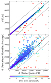 |
Fig. B.1. Comparison between distances derived from Gaia. In the top panel, distances from the inverse of the parallax (corrected for the zeropoint) against the distances from Bailer-Jones et al. (2021) for the initial full sample of O9 – B9 type stars. In the bottom panel, distances from Pantaleoni González, et al. (in prep.) against those from Bailer-Jones et al. (2021). The stars are color-coded by their error over parallax from the Gaia DR3 data. In both panels, the two dotted lines indicate a deviation of ±1 000 pc. |
The comparison in the bottom panel shows in contrast that the difference between the distances from Pantaleoni González, et al. (in prep.) and from Bailer-Jones et al. (2021) is less than 500 pc extend only up to ∼1 500 pc, with an overall trend toward shorter distances for Bailer-Jones et al. (2021) above that distance. Above that distance, the larger scatter is also clear, which also applies to stars with a very low error over parallax. In this case, stars with larger errors also have larger discrepancies, but we attribute this to the particular cases mentioned above that affect the reliability of the initial data. As a conclusion, the prior used in Pantaleoni González, et al. (in prep.) gives larger distances as a function of the distance itself, populating the sample of stars up to ∼4 000 pm rather than ∼3 000 pc as in Bailer-Jones et al. (2021). If this is correct, it would imply that on the one hand, we might miss fewer stars than previously shown in Fig. 12 between 1 000 – 3 000 pc, which therefore increases our completeness. On the other hand, it would also imply that we may miss additional stars that would move up in the green area in Fig. 11, which therefore would likely increase our number of missing stars.
Appendix C: Examples of SB2+ systems
As described in Sect. 3.2.2, we searched the available multi-epoch spectra for new or previously identified SB2 or SB3 systems. Figure C.1 includes some example SB2+ systems that we found within the available spectra.
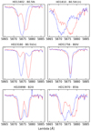 |
Fig. C.1. He Iλ5875.62 Å line for six SB2 systems identified in this work. The top two panels show two cases of lines that are blended with short separation. The middle right panel shows an example of a fast-rotating star with a normal-rotating star. Bottom panels: Easiest examples of SB2 where the lines from each star are widely separated. |
Appendix D: New spectral classifications
Table D.1 and Table D.2 include new or reviewed spectral classification based on visual morphological features for two groups of stars. The first table includes new classifications for all LC I stars with log(ℒ/ℒ⊙) < 3.5 dex from Fig. 5 that were incorrectly classified as such, and independently from the FW3414(Hβ). It also includes at the bottom some other LC II stars with log(ℒ/ℒ⊙) < 3.5 dex for which new classifications were derived or were taken from either Morgan et al. (1953, 1955) or Lesh (1968). The second table includes new classifications for stars without any spectral classification, spectral sub-type, or without LC in the default Simbad query and with FW3414(Hβ) < 7.5 Å.
New spectral classifications for some stars with LCs I and II and FW3414(Hβ) < 7.5 Å taken from Fig. 5.
New spectral classifications for the stars with FW3414(Hβ) < 7.5 Å without any spectral classification, spectral sub-type, or without luminosity class.
Appendix E: Further notes about the completeness
In Sect. 4.2.3 we provided some information about the usability of the ALS III as a reference catalog in which to check the completeness of our sample of stars up to a given distance. Figure E.1 shows the apparent magnitudes of a set of stars covering the space of SpT and LC in our sample against different distances and for two values of total extinction, Av = 0 and Av = 8. There, we indicate three threshold magnitudes at mv = 9, 11, and 16. The first and second constrain the magnitudes that are hardly (but not impossibly) accessible from the observing facilities we used to build this sample, while the latter corresponds to the magnitude from which point the ALS III catalog may begin to miss start. At mv = 16, in the case of Av = 0 (highly ideal), we would be able to observe all stars up to even 4 000 pc with an apparent magnitude mv < 9. However, as pointed out in Sect. 4.2.3, the extinction in the Milky Way can be severe in certain sight lines (Av > 4). When we focus on distances below 2 000 pc, no stars would be missing even at Av = 8. However, we refer to Fig. 5, which shows that the coldest LC II-III stars above log(ℒ/ℒ⊙) = 3.5 dex lie below the 20 M⊙ track, which indicates that these stars likely do not evolve from the O-type stars. When we take this into account, we could extend the maximum value of Av up to Av = 10 – 13 (for LC I), where still we would not expect to miss many BSGs, except for for those that are extremely reddened.
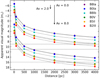 |
Fig. E.1. Apparent magnitude against distance for a set of six stars with different SpT and LC and for Av = 0, and Av = 8. Three threshold magnitudes at mv = 9, 11, 16 are indicated (see Appendix E). Two extinction vectors are also included. |
Appendix F: Hypergiant stars
List of hypergiants stars we found in the sample of O9 – B9 stars. The table includes the identifier of the star together with the Simbad default classifications and those adopted in this work.
As indicated in Sect. 4.1, we include here the list of hypergiants we found within the sample of O9 – B9 stars, independently of whether the Hβ with difference was measurable or not.
The selection was made by filtering the full sample by stars with the PCy++ label in the Hβ line profile, according to the morphological classification described in Sect. 4.2.5. Their classifications were revised and are included together with the default classifications from Simbad.
Appendix G: Comparison of the line-broadening
We compared our results for the v sin i and those obtained with the Radial Velocity Spectrometer (R ≈ 11 500) on board Gaia to account for the line-broadening (Vbroad). As pointed out in Frémat et al. (2023), the parameter Vbroad does not account for other mechanisms affecting the line profiles, neither for the macroturbulence (e.g., Aerts et al. 2009; Simón-Díaz et al. 2010), which is assumed to be 0 km s−1, nor for the microturbulence (e.g., Cantiello et al. 2009; Grassitelli et al. 2015) as in our case. Moreover, the hottest stars for which radial velocities are derived in the DR3 reach only 14 500 K (Blomme et al. 2023), and therefore, we did not expected to obtain accurate measurements of Vbroad but only a rough estimate. Figure G.1 compares the two measurements for the sample of O9 – B9 stars with a FW3414(Hβ) < 7.5 Å, excluding those with a poor determination of v sin i (see Sect. 4.3) and the SB2+. We note that only ∼15% of the stars had values of Vbroad. The comparison shows that on the one hand, only very few stars had values for Vbroad above v sin i ≳ 70 km s−1 compared to the number of stars with v sin i above that value (see Fig. 15), but for stars with v sin i ≳ 120 km s−1, the agreement is lower than 10 km s−1. On the other hand, the O9 – B4 stars with v sin i ≲ 70 km s−1 have systematically higher values of v sin i with differences ≳120 km s−1 in several cases, thus indicating that in this domain, the values for Vbroad are not reliable. The only case in which the results from Vbroad are similar to ours correspond to the late-B stars with v sin i ≲ 40 km s−1.
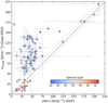 |
Fig. G.1. Comparison of the projected rotational velocity derived from the Goodness of Fit method (v sin i) and the line-broadening parameter (Vbroad) from Gaia for the sample of O9 – B9 stars with a FW3414(Hβ) < 7.5 Å. The stars are color-coded by spectral type. The three dashed lines indicate the 1:1 line for comparison and the additional two lines are shifted by ±10 km s−1. |
Appendix H: Long tables
Summary of information for the sample of stars.
Photometric and kinematic data from Gaia.
Photometric and kinematic data from HIPPARCOS.
All Tables
New spectral classifications for some stars with LCs I and II and FW3414(Hβ) < 7.5 Å taken from Fig. 5.
New spectral classifications for the stars with FW3414(Hβ) < 7.5 Å without any spectral classification, spectral sub-type, or without luminosity class.
List of hypergiants stars we found in the sample of O9 – B9 stars. The table includes the identifier of the star together with the Simbad default classifications and those adopted in this work.
All Figures
|
Fig. 1. Subsample of 246 Galactic O- and B-type stars investigated by Simón-Díaz et al. (2017), color-coded by the LC taken from Simbad. Left panel: location of the stars in a spectroscopic Hertzsprung-Russel diagram (see Sect. 3.1.1). The rough boundary between the O- and B-type star domains is indicated with the dotted diagonal black line. The evolutionary tracks taken from the MESA Isochrones & Stellar Tracks online tool for solar metallicity, and no initial rotation are included for reference purposes. Right panel: log(ℒ/ℒ⊙) against FW3414(Hβ) for the same stars. The vertical dashed red line and dashed horizontal black lines at log(ℒ/ℒ⊙) = 3.5 dex in both panels are included for reference (see Sect. 4.1). |
| In the text | |
|
Fig. 2. Results from testing the method described in Sect. 3.1.2 measuring the FW3414(Hβ). Top panel: four illustrative Hβ profiles named A, B, C, and D for FASTWIND models with Teff = 24 000 K and R = 25 000, and different pairs of log g and v sin i. The horizontal pink lines indicate the position at three-quarters, one-half, and one-quarter of the line depth for example D. Middle and bottom panels: log(ℒ/ℒ⊙) against FW3414(Hβ) and FWHM, both measured in a grid of synthetic Hβ profiles from FASTWIND with the same Teff and R as in the top panel, and values of v sin i between 10 and 360 km s−1. The four profiles in the top panel are indicated with open circles and letters. The error bars in the middle panel show the average shift in all measurements due to the effect of different resolutions, and the effect of increasing Teff up to 30 000 K (approximate temperature for a B0 I–II star). |
| In the text | |
|
Fig. 3. Examples of different Hα profiles found within our sample. The name of the stars and spectral types and morphological labels (see Sect. 3.2.1) are included. The spectra are corrected for radial velocity by using a set of photospheric metal lines. The vertical dashed red lines indicate the reference position of the line. |
| In the text | |
|
Fig. 4. Histogram of the number of stars in bins of FW3414(Hβ) for the initial sample of O9 – B9 type stars. In each bin, the number of stars is stacked by luminosity class with different colors. The spectral classifications have been taken from Simbad. The sources without a luminosity class are grouped in pink under the label “No inf.”. Independent of their LC, all stars classified as SB2+ are grouped in bins in gray. |
| In the text | |
|
Fig. 5. Preliminary results from the quantitative spectroscopic analysis of ≈500 O9–B6 type stars presented in this work for which the FW3414(Hβ) has been measured. The color code in both panels indicates the LC taken from Simbad. Left panel: sHRD for these stars and additional results from Holgado et al. (2018), indicated with gray dots. The evolutionary tracks are taken from the MESA Isochrones & Stellar Tracks online tool for solar metallicity and no initial rotation. The approximate separation between O- and B-type stars is indicated with the dotted diagonal black line. The dashed horizontal black line at log(ℒ/ℒ⊙) = 3.5 dex used in the selection of the working sample is indicated (also shown in the right panel). Right panel: log(ℒ/ℒ⊙) against FW3414(Hβ) for the same ≈500 stars. The vertical dashed red line shows the value we adopted to select the working sample. Open circles indicate stars with v sin i > 120 km s−1, and gray crosses are SB2+ systems. Stars without luminosity classes in Simbad are plotted in pink. |
| In the text | |
|
Fig. 6. Histogram of the number of stars in bins of spectral types for the final sample of stars. In each bin, the number of stars is stacked by luminosity class with different colors. Independent of their LC, all stars classified as SB2+ are stacked in gray bins. |
| In the text | |
|
Fig. 7. Stacked histogram of the number of stars in bins of 200 pc for the final sample of stars up to 4000 pc. The distances were obtained either from Bailer-Jones et al. (2021; blue bins) or using the inverse of the parallax from HIPPARCOS for stars without Gaia DR3 data (orange bins). The latter are limited to those with σϖ/ϖ ≤ 0.1. |
| In the text | |
|
Fig. 8. Polar plot in Galactic coordinates of the stars in the final sample, centered at the position of the Sun and up to a distance of 4 kpc. The stars are colored by the σϖ/ϖ parameter between 0% and 25%. Stars with distances taken from HIPPARCOS are limited to those with σϖ/ϖ ≤ 0.1. |
| In the text | |
|
Fig. 9. Histogram of the number stars in the sample with the Bmag magnitude for the stars in the sample in bins of 0.5 mag. Stars with distances taken from HIPPARCOS with σϖ/ϖ ≤ 0.1 are indicated in orange. |
| In the text | |
|
Fig. 10. Gaia DR3 Gmag corrected for distance against GBP − GRP for the selected sample, color-coded with the LC. The solid black line shows the ZAMS. The evolutionary tracks for 9, 15, 20, and 40 M⊙ up to the end of the He-burning phase obtained from MESA without initial rotation or extinction are shown in gray. No reddening is applied. Instead, a reddening vector with Δ(Av) = 1 is indicated with the red arrow. Two diagonal dashed black lines show two extinction lines for a 20 M⊙ star and for the approximate position in Fig. 5 in which the same track crosses the value of log(ℒ/ℒ⊙) ≈ 3.5 dex, respectively. |
| In the text | |
|
Fig. 11. Same as Fig. 10, but now including O9 to B9 stars from the ALS III catalog (Pantaleoni González et al., in prep.) limited to stars Bmag < 11, and distances of 4000 pc. The two diagonal dashed black lines mark the reddening line of a 20 M⊙ star. They establish three regions in the diagram that are expected to be mostly correlated with log(ℒ/ℒ⊙), as described in Sect. 4.2.2. The bottom line starts from the ZAMS, and the top line starts from the approximate age at which it intersects the horizontal dashed black line in the left panel of Fig. 5 at log(ℒ/ℒ⊙) = 3.5 dex. Both extended up to a Δ(Av) = 2. The stars in the full sample of observed O9–B9 type stars for which the upper and lower distances based on the errors lie above the top reddening line are shown in green, those for which one of the distances lies between the two reddening lines are shown in blue, and those for which one of the distances lies below the bottom reddening line are shown in red. The remaining stars populating the CMD are plotted in gray and correspond to stars that are not yet observed. Four tracks from MESA with Av = 0.0 and no initial rotation are included for 9 M⊙, 15 M⊙, 20 M⊙, and 40 M⊙. |
| In the text | |
|
Fig. 12. Histogram summarizing the completeness of the sample respect to the ALS III catalog for stars above the top reddening line of Fig. 11 (see Sect. 4.2.3 for more details), in bins of 250 pc of distance. Observed O9 – B9 stars are in green, while missing stars from the ALS III are colored in two gray colors: in dark gray, missing stars with Bmag < 9, and in light gray, stars with 9 < Bmag < 11. For each group, hatched areas indicate those stars with GBP − GRP > 0.5. |
| In the text | |
|
Fig. 13. Two polar plots in Galactic coordinates of all the stars above the top reddening line of Fig. 11, separating in the top and bottom panels those with GBP − GRP ≶ 0.5. In both panels, light gray or gray circles indicate missing stars separating those with 9 < Bmag < 11 or Bmag < 9, respectively, and with green circles the stars for which spectroscopic data are available. |
| In the text | |
|
Fig. 14. Results of the number of stars against their spectral type (two leftmost panels) and luminosity class (two rightmost panels), represented in histograms. Each bin stacks the number of stars with different morphologies found for the Hβ and Hα profiles following the classification in Sect. 3.2.1 and grouped as in the legend. Stars labeled within the “Absorption” label include profiles CF, DsP, PCy, and RF. The sources with LC I without subtype in the literature are grouped into a separate bin. The sources classified as SB2+ are removed from the bins. |
| In the text | |
|
Fig. 15. Histogram and cumulative distribution of the v sin i in the sample stars, excluding the identified SB2+ stars. In the top panel, each bin of the histogram is 20 km s−1 wide and stacks the stars separated and color-coded by their LC. In the bottom panel, we plot the cumulative distributions separated by LCs. |
| In the text | |
|
Fig. 16. Main panel: distribution of the median of v sin i obtained through the GoF method of IACOB-BROAD against the SpT, separated into stars with LCs I and II. The solid error bars indicate the upper and lower limits corresponding to the 75% and 25% percentiles, and the dashed error bars correspond to 90% and 10% percentiles. Stars without LC or SB2+ systems are not included. Small panel: histogram of the subsample of B1 I–II stars against the v sin i for a better interpretation of the main paneland Sect. 4.3. The error bars corresponding to the B1 I–II stars are plotted horizontally. |
| In the text | |
|
Fig. B.1. Comparison between distances derived from Gaia. In the top panel, distances from the inverse of the parallax (corrected for the zeropoint) against the distances from Bailer-Jones et al. (2021) for the initial full sample of O9 – B9 type stars. In the bottom panel, distances from Pantaleoni González, et al. (in prep.) against those from Bailer-Jones et al. (2021). The stars are color-coded by their error over parallax from the Gaia DR3 data. In both panels, the two dotted lines indicate a deviation of ±1 000 pc. |
| In the text | |
|
Fig. C.1. He Iλ5875.62 Å line for six SB2 systems identified in this work. The top two panels show two cases of lines that are blended with short separation. The middle right panel shows an example of a fast-rotating star with a normal-rotating star. Bottom panels: Easiest examples of SB2 where the lines from each star are widely separated. |
| In the text | |
|
Fig. E.1. Apparent magnitude against distance for a set of six stars with different SpT and LC and for Av = 0, and Av = 8. Three threshold magnitudes at mv = 9, 11, 16 are indicated (see Appendix E). Two extinction vectors are also included. |
| In the text | |
|
Fig. G.1. Comparison of the projected rotational velocity derived from the Goodness of Fit method (v sin i) and the line-broadening parameter (Vbroad) from Gaia for the sample of O9 – B9 stars with a FW3414(Hβ) < 7.5 Å. The stars are color-coded by spectral type. The three dashed lines indicate the 1:1 line for comparison and the additional two lines are shifted by ±10 km s−1. |
| In the text | |
Current usage metrics show cumulative count of Article Views (full-text article views including HTML views, PDF and ePub downloads, according to the available data) and Abstracts Views on Vision4Press platform.
Data correspond to usage on the plateform after 2015. The current usage metrics is available 48-96 hours after online publication and is updated daily on week days.
Initial download of the metrics may take a while.