| Issue |
A&A
Volume 674, June 2023
|
|
|---|---|---|
| Article Number | A206 | |
| Number of page(s) | 11 | |
| Section | Planets and planetary systems | |
| DOI | https://doi.org/10.1051/0004-6361/202345989 | |
| Published online | 26 June 2023 | |
Coma environment of comet C/2017 K2 around the water ice sublimation boundary observed with VLT/MUSE★
1
Institut für Geophysik und Extraterrestrische Physik, Technische Universität Braunschweig,
Mendelssohnstr. 3,
38106
Braunschweig, Germany
e-mail: y.kwon@tu-braunschweig.de
2
Institute for Astronomy, University of Edinburgh, Royal Observatory,
Edinburgh,
EH9 3HJ, UK
3
INAF – Osservatorio Astrofisico di Arcetri -
Largo Enrico Fermi, 5,
50125
Firenze, Italy
Received:
24
January
2023
Accepted:
2
May
2023
We report a new imaging spectroscopic observation of Oort cloud comet C/2017 K2 (hereafter K2) with the Multi Unit Spectroscopic Explorer (MUSE) instrument at the Very Large Telescope on its way to perihelion at 2.53 au, around a heliocentric distance where H2O ice begins to play a key role in comet activation. Normalized reflectances over 6500–8500 Å for its inner (cometocentric distance ρ ≈ 103 km) and outer (ρ ≈ 2 × 10⁴ km) comae are 9.7 ± 0.5 and 7.2 ± 0.3 % (103 Å)−1, respectively, the latter being consistent with the slope observed when the comet was beyond the orbit of Saturn. The dust coma of K2 at the time of observation appears to contain three distinct populations: millimeter-sized chunks prevailing at ρ ≲ 103 km; a 105 km steady-state dust envelope; and fresh anti-sunward jet particles. The dust chunks dominate the continuum signal and are distributed over a similar radial distance scale as the coma region with redder dust than nearby. They also appear to be co-spatial with OI1D, suggesting that the chunks may accommodate H2O ice with a fraction (≳1%) of refractory materials. The jet particles do not colocate with any gas species detected. The outer coma spectrum contains three significant emissions from C2(0,0) Swan band, OI1D, and CN(1,0) red band, with an overall deficiency in NH2. Assuming that all OI1D flux results from H2O dissociation, we compute an upper limit on the water production rate QH2O of ~7 × 1028 molec s−1 (with an uncertainty of a factor of two). The production ratio log[QC2/QCN] of K2 suggests that the comet has a typical carbon chain composition, with the value potentially changing with distance from the Sun. Our observations suggest that dust chunks (>0.1 mm) containing water ice and near K2’s nucleus emitted beyond 4 au may be responsible for its very low gas rotational temperature and the discrepancy between its optical and infrared lights reported at similar heliocentric distances.
Key words: comets: general / comets: individual: C/2017 K2 / methods: observational / methods: numerical / techniques: imaging spectroscopy / techniques: photometric
© The Authors 2023
 Open Access article, published by EDP Sciences, under the terms of the Creative Commons Attribution License (https://creativecommons.org/licenses/by/4.0), which permits unrestricted use, distribution, and reproduction in any medium, provided the original work is properly cited.
This article is published in open access under the Subscribe to Open model. Subscribe to A&A to support open access publication.
1 Introduction
Comets are among the least altered planetesimals in our Solar System. They consist of dust and ice. Sublimation of ice entrains dust and gas molecules, forming a cometary coma whose development is primarily determined by the nature of its nucleus. As such, identifying activity provides valuable insight into the characteristics of the building blocks that make up comet nuclei.
Comet C/2017 K2 (PANSTARRS) (hereafter K2) is an active Oort cloud comet; in July 2022 it crossed heliocentric distances of ~2.5–3.0 au from the Sun, where the main trigger of comet outgassing transitions from supervolatile ices to H2O ice (known as the water ice sublimation boundary; Blum et al. 2014; Womack et al. 2017; Gundlach et al. 2020). K2 already developed a 105 km-scale coma beyond Saturn (Jewitt et al. 2017) that would be initiated in the Kuiper belt (Jewitt et al. 2021). With a dust production rate up to ~ 103 times that of most comets at similar distances from the Sun (e.g., Garcia et al. 2020), K2 offers a unique opportunity to study an activity regime previously not observed in detail.
During the monitoring of K2 as it crossed over the water ice sublimation boundary, observations with ESO/CRIRES+, the cryogenic infrared Echelle spectrograph, at the beginning of July revealed an unexpected discrepancy at about 2.7 au. Despite the brightness and expected activity of the comet, the infrared emission features of gas molecules and dust continuum are barely discernible except for a few faint lines of CO (Fig. 1, Lippi et al. 2022, and in prep.), CH4, and C2H6 compared to what is expected from their optical counterparts (Jehin et al. 2022). For comets in general, the infrared domain over ~3–5 µm contains fundamental fluorescence emissions from molecules that are released directly from the nucleus known as primary or parent molecules (e.g., H2O, CH4, CO, and CH3OH; Bockelée-Morvan et al. 2004), superimposed on a combination of solar-reflected light and thermal dust continuum. As the molecules move outward from the nucleus, they interact with solar photons and become photo-dissociated. The photo-dissociated products, known as secondary or daughter molecules (e.g., C2, NH2, and CN; Feldman et al. 2004), produce emission features in the optical domain over ~0.4–1.0 µm. Bright emissions from daughter molecules usually indicate the presence of corresponding parent molecules in the infrared (Mumma & Charnley 2011; Biver et al. 2022); for example, a large amount of OH measured in the optical should correspond to a similar amount of its parent molecule H2O sampled in the infrared. In this regard, the observed discrepancy in K2 would suggest an alternative source for the observed daughter molecules rather than ice embedded in the nucleus or some physical processes that we are still unaware of. Moreover, the very faint thermal dust continuum suggests a low-temperature environment and dust with unusual size distributions and/or compositions.
The lack of spatially resolved information regarding what happens to comets farther from the Sun makes it difficult to determine whether the observed discrepancy is typical of comets crossing the water ice sublimation boundary or if it is unique to comet K2. Hence, we conducted one-epoch observations using the Multi Unit Spectroscopic Explorer (MUSE) at 2.53 au, where the comet is still within the same activity regime as the above-mentioned optical and infrared observations. With MUSE offering simultaneous spectral and spatial information on dust and gas coma species, our aim is to investigate how those species compose coma signals and to then suggest possible explanations for the observed discrepancy.
Geometry and instrument settings of the observations of C/2017 K2 (PANSTARRS) on UT 2022 July 29.
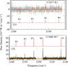 |
Fig. 1 Comparison between CO spectra of K2 (observed in July with ESO/CRIRES+) and C/2006 W3 (Christensen) (observed in October 2009 with ESO/CRIRES). The comets were at heliocentric distances of 2.75 au and 3.25 au, respectively. In both panels, the red lines indicate the CO model, while the dotted yellow lines are the ±1σ noise. C/2006 W3 (Christensen) shows very strong CO emission lines even if at a larger heliocentric distance than K2 (bottom panel, adapted from Bonev et al. 2017), while CO lines for K2 are at the noise level (top panel, Lippi et al., in prep.). |
2 Observations and data analysis
This study is based on single-epoch data carried out under the program (ID: 109.24F3.001) of the Director’s Discretionary Time of the European Southern Observatory (ESO).
2.1 Observations
MUSE is an Integral Field Unit (IFU) spectrograph mounted on the UT4 telescope of the Very Large Telescope (VLT) at the Paranal Observatory (70°24′10.″1W, 24°37′31.″5S, 2 635 m) in Chile (Bacon et al. 2010). MUSE in Wide Field Mode (WFM)1 splits a field of view (FoV) of 1′ × 1″ into 24 channels that are further sliced into 48 slitlets, each sampling 15″ × 0.″2 without adaptive optics (WFM-noAO mode) with a pixel resolution of 0.″2. Each slice offers a medium-resolution (1.25 Å interval) spectrum over the nominal wavelength coverage of 4800–9300 Å. Separate sky observations were taken at positions ≲550″ from the nucleus for every two target observations in the order O-S-O-O-S-O, where O and S denote object and sky exposure, respectively. A combination of sky acquisition and +90° position angle rotations averages out optics-induced signals, rejects cosmic rays, and thus improves the signal-to-noise ratio. We conducted a 1.5-h observation for K2 on UT 2022 July 29. The atmospheric seeing ranged from ~0.″4 to 1.″2; the maximum was an instant peak, otherwise seeing remained at ~0.″5 most of the time. A journal of observations is given in Table 1.
2.2 Data analysis
The basic data reduction (i.e., bias and sky subtraction, flat-fielding, wavelength and flux calibration, and telluric absorption correction) and construction of 3D cubes were all conducted via the ESO/MUSE Data Reduction Pipeline (DRP; Weilbacher et al. 2020). A standard star observed on the same night as our observation was used for sky subtraction and telluric correction. Since DRP corrects first-order telluric line features to satisfactory levels (e.g., the strongest O2 telluric line at ~7600 Å is well canceled out in Fig. 2a), we did not apply further modeling. The resulting seven cubes (the eighth cube was discarded due to its high airmass and incomplete FoV coverage) showed no rotational variation in the coma morphology. We therefore median combined them with a 5σ clipping using the open-source software, MUSE Python Data Analysis Framework (mpdaf)2. In the following, all results are based on the quantities derived from the median-combined cube.
A different methodology was applied for the analysis of the oxygen lines described in Sect. 3.3. Oxygen-forbidden lines at 5577, 6300, and 6364 Å are also present in the sky. At the spectral resolution of MUSE, we cannot resolve the telluric and cometary lines. In order to exploit the information contained in those lines, we ran a separate data reduction without applying any sky subtraction. For this analysis, all eight data cubes are considered separately.
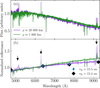 |
Fig. 2 Spectral information of K2 extracted over two different aperture radii. (a) Unbinned spectrum of the K2 coma (with a step of 1.25 Å) extracted over smaller (corresponding to the cometocentic distance ρ of ≈103 km; green) and larger (ρ ≈ 2 × 10⁴ km; purple) radius circular apertures. (b) Relative reflectance of K2 normalized at 6000 Å. Its spectra are binned to match the spectral resolution (5 Å) of the solar spectrum. Three arrows indicate significant emission features of gas species: the C2(0,0) band at ~5100 Å, the OI1D line at 6300 Å, and the CN(1,0) red band at ~9200 Å. The circles and diamonds are the data of K2 taken at rH ~15.5 and ~15.4 au, respectively (Meech et al. 2017). |
3 Results
This section examines the dust and gas coma environments in K2. The general circumstances are introduced first, followed by descriptions of each coma component.
3.1 General outlines
Figure 2 shows spectra of K2 extracted over two different aperture radii, each corresponding to the cometocentric distance ρ ≈ 103 km (inner coma, green) and 2 × 10⁴ km (outer coma, purple). The OI1D 1D–3P line at 6300 Å and the CN A2Π–X2Σ+ (1,0) red band at ~9200 Å are evident in both the inner and outer coma regions, while the C2 d3Πg–a3Πu (0,0) Swan band at ~5100 Å is discernible only in the outer part, possibly due to dust contamination. The NH2  band signals that are expected to be present over 5600–7400 Å are negligible as a whole.
The extracted spectra were then divided by the reference solar spectrum taken at an airmass of 1.5 provided by the American Society for Testing and Material3 and binned to match the spectral resolution (5 Å) of the solar spectrum. In spite of a slight mismatch in airmass between the two spectra, the resultant reflectance (Fig. 2b) provides a useful measurement of K2’s gross dust color. Dust in both coma regions is redder than the Sun, slightly concaving down at longer wavelengths. The inner coma is redder than the outer coma: fitted linearly over 6500–8500 Å, the normalized reflectivity S ′ (Jewitt & Meech 1986) is 9.7 ± 0.5 and 7.2 ± 0.3% (103 Å)−1 for the inner and outer comae, respectively. Both S are slightly bluer than, for instance, 2I/Borisov (Bannister et al. 2020) and 67P/Churyumov-Gerasimenko (Snodgrass et al. 2016) at similar heliocentric distances in their inbound orbits, but well in the average range of Solar System comets (Solontoi et al. 2012). The outer coma slope is consistent with that obtained at 15.5 and 15.4 au from the Sun (diamonds and circles covering ρ ~ 56 000 km in Fig. 2b; Meech et al. 2017), indicating that the large-scale coma has remained relatively constant.
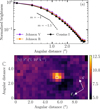 |
Fig. 3 Radial profiles of normalized brightness in standard VRI broad-bands showing possible association with the reddened coma region. (a) Azimuthally averaged radial profiles of K2 in the Johnson V and R and Cousins / filters. Two guidelines with the slope of −1 and −1.5 are plotted for comparison. (b) Map of the normalized reflectivity S′. A 2 × 2 binning is employed such that each pixel covers 0.″4. The red plus sign (+) indicates the optocenter. The negative velocity (−v) and anti-sunward (r⊙) vectors are given. North is up; east is to the left. |
3.2 Dust coma environment: Three distinct populations
We first created coma images of K2 by integrating the flux bracketed by three broadband filters V, R, and / whose azimuthally averaged radial profile is shown in Fig. 3a. The expected slope ranges for steady-state coma (−1 and −1.5; Jewitt & Meech 1987) are plotted for comparison. The two profiles are similar, and show a shallower slope than −1 from the center out to ~4 pixels (corresponding to ρ ~ 103 km) followed by a steady decrease4. In a 2 × 2-binned S′ distribution (Fig. 3b), this central region of shallow radial profile corresponds to the coma region on a scale of ρ ≈ 103 km having redder colors than the outer coma, with a lack of large-scale asymmetry. The flux originating from this reddened region is distributed on a radial scale similar to the bright central areas in continuum and gas-emitting signals (Fig. A.1a). We refrain from making a definitive statement regarding the alignment of this feature since the binned image here shows its slight sunward extension, but not the original image. The red dust color accompanied by continuum enhancement suggests that the dust clusters in this near-nucleus area are possibly dark (containing abundant carbonaceous materials such as typical cometary dust; Levasseur-Regourd et al. 2018; Filaccione et al. 2020), consolidated, large chunks that are less sensitive to solar radiation pressure (Hadamick & Levasseur-Regourd 2009; Kwon et al. 2022a). We discuss the implications of this in Sect. 4.
Next, we investigated any asymmetric structure embedded in the outer envelope by dividing out an azimuthal median profile from a broadband image (Samarasinha et al. 2013). To this end, we utilized a zg-band image of K2 from the Zwicky Transient Facility5 (ZTF) archive (Masci et al. 2019) taken on the nearest date (rH ~ 2.55 au on UT 2022 July 26) from our observation, as the MUSE's FoV is not wide enough to examine macroscopic coma structures. Figure 4a presents the ZTF image before enhancement. At first glance, the tail edge of the comet appears sharp along its negative velocity direction. This feature is indicative of the protracted ejection of large dust particles (their large inertia anchors them to the comet position from which they were released; e.g., Ishiguro et al. 2007), which is more pronounced in amateur images taken near perihelion6. Figure 4b presents the enhanced image showing a conspicuous anti-sunward jet that curves into the negative velocity direction at its outer end. Its lack of spatial correlation with gas species detected (Sect. 3.3) suggests that this feature is probably dusty. We replicate this enhanced feature of K2 using a Finson-Probstein mechanism (Finson & Probstein 1986; Burns et al. 1979) assuming zero ejection velocity where inward solar gravity forces (Fgrav)and outward solar radiation pressure (Frad) determine dust trajectory in the outer coma. Using Eq. (1) and constants in Kwon et al. (2022b), we calculate a parameter β (a ratio of Frad to Fgrav) that demonstrates the relative importance of solar radiation pressure on dust and is directly related to dust density and size. We specify each coma location with a combination of a synchrone (each represents dust with different β but ejected at the same epoch) and syndyne (each represents dust with the same β but ejected at a different epoch) so as to compare their distribution with the observed coma morphology. For this modeling, we consider a range of ejection epochs from ~180 days (>4.1 au, well beyond the water ice sublimation boundary) to one day prior to our observation, while testing dust with β from 1 down to 10−4. Additional forces that can alter dust motions in the coma (e.g., gas drag force, sublimation of embedded ice, and dust fragmentation) are not considered here.
Figure 4c shows the synchrones and syndynes plotted over the enhanced image, along with the ejection times and values considered. Dust with β of 10−4 (the smallest value tested, on the order of millimeters) is not plotted here because its extension is too short to be distinguished from the nucleus position on the given FoV. Only dust ejected recently (<5 days, at best ~1 day prior to the observation) and with high mobility (ß ≳ 0.3) is capable of reproducing the jet's position angle. However, the southern-southeastern distribution of the anti-sunward dust spread that even sufficiently small particles cannot reproduce (ß = 1, on the order of 0.1 µm), strongly indicates that our simple assumption of zero ejection velocity does not hold, and thus requires invoking nonzero initial speeds, such as rocket force from sublimating ice particles (Kelley et al. 2013). Nevertheless, given that there is no evidence of dust being redistributed immediately in the anti-sunward direction by solar radiation pressure with the end of the jet curving into the negative velocity direction, dust composing this jet feature may share properties similar to dust on a tail along the negative velocity direction (i.e., on the order of millimeters). We confirmed the presence of a similar feature in the zg- and zr-band ZTF images taken on UT 2022 August 15.
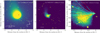 |
Fig. 4 Analysis of K2 coma morphology using its ZTF zg-band archival image, (a) Unenhanced image of K2 on UT 2022 July 26, with the vector notation used in Fig. 3. The red plus sign (+) indicates the position of the nucleus as defined by the peak flux, (b) Image enhanced by dividing out of an azimuthal median profile (Samarasinha et al. 2013). (с) Synchrones and syndynes of the K2 coma. The red dashed lines are synchrones, indicating the locations of dust ejected at 1, 5, 15, 30, 60, 90, 120, and 180 days prior to the ZTF observation (from bottom to top). The cyan curves are syndynes, where each has a constant β of 1, 0.3, 0.1, 0.03, 0.01, 0.003, and 0.001 (clockwise from the bottom). A nonzero initial outflow velocity is required to explain dust spreading from south to southeast, which is not explained by the combination of dust parameters tested. Brightness levels were arbitrarily adjusted on a linear scale to highlight each image’s coma feature of interest. |
3.3 Gas coma environment
3.3.1 Ol1 D forbidden lines
Forbidden oxygen lines at 5577.339, 6300, and 6363.776 Å have been observed in a large number of comets, usually using high-resolution spectrographs. Since we cannot separate the cometary and telluric contributions at the spectral resolution of MUSE, we used a combination of spatial and spectral information to exploit the information contained in these oxygen lines. Following the methodology described in Opitom et al. (2020), we used dat-acubes for which the sky was not subtracted to create maps of the spatial distribution of the (dust-subtracted) flux in the three oxygen lines (Fig. A.3). These maps show the contribution of the comet as a peaked contribution decreasing relatively rapidly, overplotted on a constant contribution from the sky. To produce the maps of the 5577.339 and 6363.776 Å lines, we re-centered and co-added the individual maps from seven datacubes. The sky contribution was then measured and subtracted using an annulus of 2″ width at 20″ from the comets. For the 6300 Å line we found that the emission filled the FoV in some cases. We thus only combined four maps for which the comet was offset from the center of the field (due to centering issues during the observations) and for which the sky contribution could be measured at the edge of the image. For this case the sky was measured from al″ aperture at the lower right edge of the field, which was part of the map free from comet emission.
We measured the intensity ratio of the green line to the sum of the two red lines (G/R) in two circular apertures for all maps and obtain G/R = 0.17 + 0.02 in a 1″ radius aperture and G/R = 0.13 ± 0.02 in a 2″ radius aperture. This technique can only produce an estimate of the G/R ratio, as at the spectral resolution of MUSE, we cannot exclude contamination from C2 in our measurement of the 5 577.339 Å line. However, in the case of these observations of K2, the C2 emission from the (1,0) band is faint and only detected when the extraction is done with a sufficiently large aperture. Our measurements are consistent with what is measured at similar heliocentric distances by Decock et al. (2013) and with the effect of quenching that leads to higher G/R ratios in small apertures (Decock et al. 2015). Given that a G/R of ~0.1 is expected in purely H2O-driven activity with a higher value (up to ~0.35) in CO- and CO2-dominating comet activity (Decock et al. 2013, 2015), the result indicates that H2O may play a leading role at our observing epoch, though some CO or CO2 contributions cannot be ruled out.
Using the hypothesis that the OI1D line at 6300 Å is only produced by the dissociation of H2O, we can obtain a crude estimate of the water production rate. To do that, we measured the flux of the 6300 Å over a rectangular aperture (illustrated in Fig. A.3). Examination of the radial profile shows that within that aperture, the OI1D flux decreases down to the background level at the edge of the field and we are sampling all the flux from the object in that quadrant. Since this aperture only covers 1/4 of the coma, we multiplied the measured flux by 4. To derive an estimate of the water production rate, we followed the procedure described in Opitom et al. (2020) and used branching ratios for the quiet Sun from Morgenthaler et al. (2001). Assuming that we measured the full flux of the coma, we obtain a water production rate  from the OI1D 6300 Å flux of 7 × 1028 molec s−1, with an uncertainty of factor two, mainly due to the difficulty in subtracting the sky component for this very extended emission. Our
  estimate is consistent with those of active Oort cloud comets at ~2.5 au preperihelion distance (e.g., Fink 2009; Combi et al. 2018).
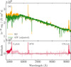 |
Fig. 5 Procedure for isolating gas emission features from the observed spectrum, (a) Unbinned spectra of K2 (orange) and 67P/Churyumov-Gerasimenko (green, from Opitom et al. 2020) whose flux and slope are adjusted to those of K2. (b) Flux residuals after subtracting the adjusted 67P spectrum from the K2. Four emission features are highlighted by thick red lines whose flux and underlying continuum images are given in Fig. A.2. Although C2(1,0) at ~5500 Å is also marginally discernible, a flux map was not created for it in this study, due to its large uncertainty following continuum subtraction. |
3.3.2 CN(1,0) and C2(0,0) bands
The signals of the CN(1,0) and C2(0,0) bands are separated by subtracting the continuum from the spectrum observed. Following Opitom et al. (2020), we employed a reference dust spectrum of comet 67P/Churyumov-Gerasimenko taken by the same instrument (MUSE), adjusted its flux and slope to match those of K2, and subtracted the reference from the K2 spectrum (the outer coma spectrum; purple in Fig. 2a). Figure 5a illustrates the adjusted reference spectrum to be subtracted. The subtraction was carried out for each pixel to produce maps of the spatial distributions of gas components.
This process leaves two significant emission signals (the C2(0,0) Swan band and CN(1,0) red band) and one fainter emission signal (OI1D 6 364 Å) (Fig. 5b). A lack of NH2 bands, particularly the NH2 band that overlaps OI1D at ~63OO Å (Fink 1994), attributes the observed feature to the latter (OI1D also appears clearly in the image without removing the sky, supporting its cometary origin; Fig. A.3). We integrated over the wavelengths highlighted in thick red in Fig. 5b, and Fig. 6 displays the resultant integrated flux distributions for the three dominant gas species. Table 2 provides information on areas of integration, their flux, and production rates, while their ancillary information (unbinned flux distributions and underlying continuum distribution) can be found in Fig. A.2 alongside the information of the OI1D 6364 Å line. Both OI1D and CN(1,0) are the strongest at the optocenter (plus signs in Fig. 6) with slight sunward extension as in the distribution of the spectral reddening (Fig. 3b). Meanwhile, C2(0,0) flux peaks consistently away from the optocenter by ~500–1000 km, which could be due in part to an oversubtraction of dust near the optocenter.
The integrated fluxes F of C2(0,0) and CN(1,0) bands over the aperture radius of 15″ (Table 2) are converted to their production rates Q using the Haser model (Haser 1957). We used conventional parameters of the model to provide Q estimates on an order-of-magnitude basis. The outflow velocity was scaled by the inverse scaling law  , where rH is the heliocentric distance (2.53 au) (Delsemme 1982). The g-factors (fluorescence efficiencies) and daughter scale lengths for CN(1,0) and C2 are from Lara et al. (2004) and A'Hearn et al. (1995), respectively, and scaled as rH−2 (for the ɡ-factors) and as rH2 (for the scale lengths). Together with the Haser correction factors provided by Schleicher (2010)7 given that our aperture does not contain the full flux for the species of interest, we compute
  of (1.1 ± 0.2) × 1026 molec s−1 and QCN of (0.7 ± 0.1) × 1026 molec s−1. The resultant Q ratio log
![$\left[ {{{{Q_{{{\rm{C}}_2}}}} \mathord{\left/ {\vphantom {{{Q_{{{\rm{C}}_2}}}} {{Q_{{\rm{CN}}}}}}} \right. \kern-\nulldelimiterspace} {{Q_{{\rm{CN}}}}}}} \right]$](/articles/aa/full_html/2023/06/aa45989-23/aa45989-23-eq8.png) is ~0.19. Our
is ~0.19. Our  and QCN estimates are consistent within 2σ and a factor of 2, respectively, with the values measured at 0.25 au farther from the Sun than our observation (Jehin et al. 2022):
  and QCN = (2.09 ± 0.13) × 1026 molec s−1.
The carbon chain composition of K2 can be compared with canonical classification criteria (A'Hearn et al. 1995). A QCN in A'Hearn et al. (1995) was measured from CN(0,0) violet band at 3880 Å, which is beyond the nominal wavelength of MUSE. The QCN in Table 2 was computed by the flux integrated over 9141–9269 Å, which is narrower than its nominal band region of ~9100–9320 Å, thereby missing part of the CN(1,0) signal. If we simply assume a Gaussian band shape of CN(1,0) over the nominal wavelength, the approximate missing fraction is ~25% of the total CN(1,0) band signal. Hence, considering that the CN violet band is generally stronger than the CN(1,0) red band (Schleicher 2010), in the end the resulting QCN of the CN violet band, calculated from its flux (a few times brighter than our FCN) and the corresponding g-factor (~3–4 times the CN(1,0) value; A'Hearn et al. 1995), may be comparable to our QCN in the end. The log ratios of the production rates log![$\left[ {{{{Q_{{{\rm{C}}_2}}}} \mathord{\left/ {\vphantom {{{Q_{{{\rm{C}}_2}}}} {{Q_{{\rm{CN}}}}}}} \right. \kern-\nulldelimiterspace} {{Q_{{\rm{CN}}}}}}} \right]$](/articles/aa/full_html/2023/06/aa45989-23/aa45989-23-eq12.png) are well within the average range of Oort cloud comets (A’Hearn et al. 1995; Fink 2009; Cochran et al. 2012) and in the typical group of comets in carbon chain composition having log
are well within the average range of Oort cloud comets (A’Hearn et al. 1995; Fink 2009; Cochran et al. 2012) and in the typical group of comets in carbon chain composition having log![$\left[ {{{{Q_{{{\rm{C}}_2}}}} \mathord{\left/ {\vphantom {{{Q_{{{\rm{C}}_2}}}} {{Q_{{\rm{CN}}}}}}} \right. \kern-\nulldelimiterspace} {{Q_{{\rm{CN}}}}}}} \right] \ge - 0.18$](/articles/aa/full_html/2023/06/aa45989-23/aa45989-23-eq13.png) (A’Hearn et al. 1995). By comparison, the log
(A’Hearn et al. 1995). By comparison, the log![$\left[ {{{{Q_{{{\rm{C}}_2}}}} \mathord{\left/ {\vphantom {{{Q_{{{\rm{C}}_2}}}} {{Q_{{\rm{CN}}}}}}} \right. \kern-\nulldelimiterspace} {{Q_{{\rm{CN}}}}}}} \right]$](/articles/aa/full_html/2023/06/aa45989-23/aa45989-23-eq14.png) value reported for K2 one month before the time of our observation is ∼−0.04 (Jehin et al. 2022). This value is still within the typical carbon chain group, but lower (i.e., carbon deficient) than our estimate, suggesting that the C2/CN ratio may change with the distance from the Sun.
value reported for K2 one month before the time of our observation is ∼−0.04 (Jehin et al. 2022). This value is still within the typical carbon chain group, but lower (i.e., carbon deficient) than our estimate, suggesting that the C2/CN ratio may change with the distance from the Sun.
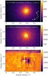 |
Fig. 6 2 × 2 binned flux distribution of (a) OI1D line, (b) CN(1,0) red band, and (c) C2(0,0) Swan band in units of 10−20 erg cm−2 s−1. The plus sign (+) indicates the optocenter. The images have the same FoV, pixel scales, and alignment directions as those in Fig. 3b. |
Areas of integration and results of spectral analysis.
4 Discussion
When compared to a handful of comets observed at similar pre-perihelion distances (rH = 2–3 au), K2’s  and QCN are in line with those of active Oort cloud comets (A’Hearn et al. 1995; Fink 2009), and overall more prominent relative to short-period comets and interstellar comet 2I/Borisov by up to three orders of magnitude (e.g., Fink 2009; Cochran et al. 2012; Snodgrass et al. 2016; Opitom et al. 2019; Bannister et al. 2020). However, while some of those comets in abundant carbon chain molecules also display a significant level of NH2 emissions, K2 lacks relevant spectral signals (Fig. 2). This apparent deficiency in NH2 is either due to a real depletion of the molecule or the temporal status, given that NH3, the possible parent molecule of NH2, can increase its production rate at a smaller heliocentric distance (e.g., Dello Russo et al. 2016).
Although our single-epoch dataset may hardly provide a clear picture of comet composition, it is worthwhile to compare K2’s characteristics (carbon chain-rich and NH2-deficient) with another CO-rich Oort cloud comet C/2016 R2 (PanSTARRS; McKay et al. 2019) that exhibits deficiencies both in NH2 and carbon chain molecules in the optical (e.g., Cochran & McKay 2018). If the NH2 deficiency of the two CO-rich comets reflects their intrinsic depletion, a lack of the availability of NH3 in the accretion stage requires their place of origin to be at least ≳5–10 au (Lodders 2004; Kurokawa et al. 2020) and to be >35 au from their CO richness (Womack et al. 2017). Lisse et al. (2022) suggest that the CO-richness today presumably pertains to the ejection time of small bodies into the Oort cloud, as earlier ejection ensures their nuclei retain inherent CO ices. In this regard, the observed difference in photo-dissociated gas molecules between the two comets that are likely to have shared similar temperature ranges may support the idea that the compositional heterogeneity in the optical is highly individual (A’Hearn et al. 1995; Cochran et al. 2012; Opitom et al. 2019).
The asymmetric coma environment around the water ice sublimation boundary suggests that K2’s nucleus surface may not be uniformly active, resulting in three distinct dust populations inhabiting different parts of the coma (Sect. 3.2): near-nucleus chunks, steady-state outer envelope, and anti-sunward jet. Only C2(0,0) aligns with the dust envelope among the three gases detected, while the other species (OI1D, and CN(1,0) red) appear co-spatial with the near-nucleus continuum enhancement (Sect. 3.3). The possible association between the dust chunks and OI1D indicates that significant amounts of H2O ice may be present in the dust. In conjunction with their coloca-tion in the coma region where dust color is redder than the average (Fig. 3b), these connections propose that the scattering medium could be dirty ice (refractory fraction of ≳1%; Mukai 1986) whose size sufficiently exceeds the wavelength of observation (Hadamick & Levasseur-Regourd 2009; Kwon et al. 2022a). This idea of large dust particles containing H2O ice is in line with a recent report of K2 in its near-infrared spectro-scopic observations that display evidence of the characteristic H2O absorption bands at 1.5 and 2.0 µm and suggest nonzero dust refractory contents in the ice particles (Protopapa et al. 2022). In our dynamical modeling of coma dust (Fig. 4c), only dust particles with low mobility (β < 0.001, >0.1 mm; Kwon et al. 2017) emitted long ago (rH > 4.1 au, released at least six months before the observation) can match the small radial scale (ρ ≲ 103 km) of the dust clustering. This millimeter-sized dust is in accordance with the size range predicted from distant cometary activity (Bouziani & Jewitt 2022) and with previous estimates of K2 at large heliocentric distances (Jewitt et al. 2017; Hui et al. 2017).
The ejection of dust containing H2O ice necessitates the sublimation of ices more volatile than H2O, such as CO2 or CO (e.g., Gundlach et al. 2020; Ciarniello et al. 2022). K2’s unprecedent-edly high coma activity beyond Saturn (Meech et al. 2017; Jewitt et al. 2017) and direct detection of CO emission at rH ~ 6.72 au (Yang et al. 2021) underpin the presence of abundant supervolatile ice in the nucleus of the comet. It is worth noting that the CO emission in K2 was headed primarily in the sunward direction (Yang et al. 2021), the same direction where dust chunks are dominating in the binned image (Fig. 3b). The presence of chunks containing H2O ice may offer a plausible answer to the observed discrepancy of K2 between optical and infrared wavelengths (Sect. 1). Around the time of our observations, the comet is still far away from the Sun (~2.5–2.7 au). Given that the lifetime of ice decreases as the temperature increases, the low temperature may hamper direct H2O ice sublimation from the nucleus. Dust of ≳100 µm in size has a sublimation lifetime of ~104–5 s (corresponding to ≳104 km for the dust of interest) at ~2.5 au (Mukai 1986). The slit width of ESO/CRIRES+ that detected no H2O emission features of small ice grains samples about 1500 km from the nucleus, that is, at distances shorter than those where sublimation takes place (Lippi et al., in prep.). On the other hand, our spectroscopic measurements and those reported at similar epochs (e.g., Jehin et al. 2022 using 0.6 m TRAPPIST robotic telescopes) have been carried out over ≳104 km from the nucleus, thereby having a much higher chance to detect the emission features of daughter molecules arising from the photo-dissociation process. In this context, the detection of absorption features of H2O ice in K2 by IRTF InfraRed Telescope Facility (IRTF)/SpeX (Protopapa et al. 2022) provides supportive evidence for the presence of dust chunks (on the order of ≳100 µm; Grundy & Schmitt 1998).
Taken altogether, the K2 coma environment investigated in this study can be interpreted as the following evolutionary scenario: dirty ice chunks entrained by supervolatile ice at very large heliocentric distances have started sublimating its internal H2O ice as the comet reaches the inner Solar System, while an anti-sunward jet has formed near the water ice sublimation boundary, presumably launched by H2O ice. Monitoring observations of this active comet during the crossing of this normal water ice sublimation boundary were conducted using optical imaging polarimetry (Kwon et al., in prep.) and infrared echelle spectroscopy (Lippi et al., in prep.). For this reason, we defer discussing K2’s secular evolution in a broader context to our future research.
5 Summary
Here we present a new IFU observation of K2 around the water ice sublimation boundary using VLT/MUSE, as part of our monitoring observation program, in conjunction with ZTF archival data. The coma appears heterogeneous, consisting of three distinct populations of dust (near-nucleus chunks, envelope, and jet distributed in sizes, colors, and possibly compositions) and three significant gas species (OI1D and C2(0,0), and CN(1,0) red bands) occupying different parts of the coma. Based on their spectral and spatial information, we discuss dust properties, abundance and production rates of the gas, and their mutual association.
If water ice-harboring large dust chunks were indeed present near the nucleus of K2, this would be compatible with the existence of water ice grains likely containing nonzero refractory content as suggested by infrared spectroscopic observations taken at similar epochs (Protopapa et al. 2022), further explaining its bare detection of dust continuum and H2O emission features (Lippi et al. 2022, and in prep.). All physical quantities derived from this study can vary as K2 travels through the inner Solar System (e.g., NH2 deficiency and  ; Cochran et al. 2012; Bannister et al. 2020). We thus expect this study to serve as a reference of cometary activity around the water ice sublimation boundary for future studies that track the secular evolution of cometary activity.
Acknowledgements
We thank Emmanuel Jehin for a useful discussion of K2 gas emissions at optical wavelengths. Based on observations made with ESO Telescopes at the Paranal Observatory under program 109.24F3.001. Y.G.K gratefully acknowledges funding from the Volkswagen Foundation. M.L. acknowledges funding from the European Union's Horizon 2020 research and innovation program under grant agreement no. 75390 CAstRA.
Appendix A Ancillary figures
Figure A.1 displays unbinned continuum and gas emission flux images acquired from the continuum subtraction. Both coma components have a strong concentration in the central part of the coma without significant large-scale asymmetry. The maps are constructed by combining the two cubes that have the smallest seeing (0.″39 and 0.″5) in our datasets. The compact distribution appears more concentric around the optocenter than a sunward extension shown in the binned images (Figs. 3b and 5). Although the binned images have less influence from the seeing effect, we cannot rule out external factors such as the centering effect of the telescope that could have led to the apparently preferred alignment. As such, we refrain from making any definitive statements regarding the near-nucleus morphology other than the strong central condensation, following our criteria (see footnote #4).
Ancillary information of the spectral analysis is available in Figure A.2. The figure summarizes unbinned flux distributions of the gas species highlighted in Figure 5b in the left column and the underlying dust continuum within the integrated wavelength interval in the right column. Both emission and continuum signals are consistent with the trends that appeared in the binned images, where most of the light from OI1D 6 300 Å line (including its OI1D doublet companion at 6 364 Å) and CN(1,0) red band come from the near-nucleus region (ρ < 103 km), while the C2(0,0) Swan band peaks off from the optocenter by ∼500−1000 km. This is also compatible with the trend that the inner coma (ρ ≈ 1 000 km) contains negligible emission features of the C2(0,0) Swan band relative to the outer coma (ρ ≈ 20 000 km; Fig. 2a). The continuum fluxes underlying each gas component distribute nearly the same, forming a compact spherical coma around the optocenter.
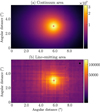 |
Fig. A.1 Unbinned flux image of (a) the continuum-emitting area and (b) the line-emitting area with contributions from all gas species. Units of axes and color bars are pixels and flux in 10−20 erg cm−2 s−1, respectively. One pixel corresponds to ρ ∼ 270 km, such that the cropped FoV covers the ∼8 100 km × 13 500 km rectangular coma region. The red plus sign (+) indicates the optocenter. The images are aligned as in Figure 3. |
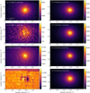 |
Fig. A.2 Maps of four gas species isolated from Figure 5. Left: Unbinned flux distribution of each gas component highlighted in Figure 5b. All fluxes are in units of 10−20 erg cm−2 s−1. The flux drop of CN(1,0) red and C2(0,0) on the top part (panels e and g) is an artifact, likely due in part to their flux in the outer coma region highly susceptible to background noise, and thus having large uncertainties in estimating the continuum signal. Right: Unbinned flux distribution of the underlying continuum integrated over the considered wavelengths. They are subtracted from the observed spectrum to offer the line flux on the left side. The red plus sign (+) indicates the optocenter. |
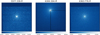 |
Fig. A.3 Maps of the three forbidden oxygen lines. The FoV is 60 × 58 ″2, and the images are oriented north up and east to the left. The 6300 Å line map is offset with respect to the other two maps since the spatial extension of the emission is larger, and only off-centered observations were used. The black box illustrates the aperture used for the measurement of the water production rate. |
References
- A’Hearn, M. F., Millis, R. L., Schleicher, D. G., Osip, D. J., & Birch, P. V. 1995, Icarus, 118, 223 [Google Scholar]
- A’Hearn, M. F., Belton, M. J. S., Delamere, W. A., et al. 2011, Science, 332, 1396 [CrossRef] [Google Scholar]
- Bacon, R., Accardo, M., Adjali, L., et al. 2010, Proc. SPIE, 7735, 773508 [Google Scholar]
- Bannister, M. T., Opitom, C., Fitzsimmons, A., et al. 2020, AAS J., submitted [arXiv:2001.11605] [Google Scholar]
- Biver, N., Dello Russo, N., Opitom, C., & Rubin, M. 2022, Comets III (Oxford University Press) [Google Scholar]
- Bockelée-Morvan, D., Crovisier, J., Mumma, M. J., & Weaver, H. A. 2004, Comets II, eds. M. Festou, H. U. Keller, & H. A. Weaver (Tucson: University of Arizona Press), 391 [Google Scholar]
- Blum, J., Gundlach, B., Mühle, S., & Trigo-Rodriguez, J. M. 2014, Icarus, 235, 156 [Google Scholar]
- Bonev, B. P., Villanueva, G. L., DiSanti, M. A., et al. 2017, AJ, 153, 241 [NASA ADS] [CrossRef] [Google Scholar]
- Bouziani, N., & Jewitt, D. 2022, ApJ, 924, 37 [NASA ADS] [CrossRef] [Google Scholar]
- Burns, J. A., Lamy, P. L., & Soter, S. 1979, Icarus, 40, 1 [Google Scholar]
- Ciarniello, M., Fulle, M., Raponi, A., et al. 2022, Nat. Astron., 6, 546 [NASA ADS] [CrossRef] [Google Scholar]
- Cochran, A. L., & McKay, A. J. 2018, ApJ, 854, L10 [Google Scholar]
- Cochran, A. L., Barker, E. S., & Gray, C. L. 2012, Icarus, 218, 144 [Google Scholar]
- Combi, M. R., Mäkinen, T. T., Bertaux, J.-L., et al. 2018, Icarus, 300, 33 [NASA ADS] [CrossRef] [Google Scholar]
- Decock, A., Jehin, E., Hutsemékers, D., & Manfroid, J. 2013, A&A, 555, A34 [NASA ADS] [CrossRef] [EDP Sciences] [Google Scholar]
- Decock, A., Jehin, E., Rousselot, P., et al. 2015, A&A, 573, A1 [NASA ADS] [CrossRef] [EDP Sciences] [Google Scholar]
- Dello Russo, N., Kawakita, H., Vervack, R. J., & Weaver, H. A. 2016, Icarus, 278, 301 [NASA ADS] [CrossRef] [Google Scholar]
- Delsemme, A. H. 1982, Comets, ed. L. L. Wilkening (Tucson: University of Arizona Press), 85 [CrossRef] [Google Scholar]
- Feldman, P. D., Cochran, A. L., & Combi, M. R. 2004, Comets II, eds. M. Festou, H. U. Keller, & H. A. Weaver (Tucson: University of Arizona Press), 425 [Google Scholar]
- Filaccione, G., Capaccioni, F., Ciarniello, M., et al. 2020, Nature, 578, 49 [NASA ADS] [CrossRef] [Google Scholar]
- Fink, U. 1994, ApJ, 423, 461 [NASA ADS] [CrossRef] [Google Scholar]
- Fink, U. 2009, Icarus, 201, 311 [Google Scholar]
- Fink, U., & DiSanti, M. A. 1990, ApJ, 364, 687 [NASA ADS] [CrossRef] [Google Scholar]
- Finson, M., & Probstein, R. 1968, ApJ, 154, 327 [NASA ADS] [CrossRef] [Google Scholar]
- Garcia, R. S., Gil-Hutton, R., & García-Migani, E. 2020, P&SS, 180, 104779 [NASA ADS] [CrossRef] [Google Scholar]
- Grundy, W. M., & Schmitt, B. 1998, J. Geophys. Res., 103, 25809 [NASA ADS] [CrossRef] [Google Scholar]
- Gundlach, B., Fulle, M., & Blum, J. 2020, MNRAS, 493, 3690 [NASA ADS] [CrossRef] [Google Scholar]
- Hadamick, E., & Levasseur-Regourd, A.-C. 2009, Planet. Space Sci., 57, 1118 [NASA ADS] [CrossRef] [Google Scholar]
- Haser, L. 1957, Bull. Soc. R. Sci. Liege, 43, 740 [NASA ADS] [Google Scholar]
- Hui, M.-T., Jewitt, D., & Clark, D. 2017, AJ, 155, 25 [CrossRef] [Google Scholar]
- Ishiguro, M., Sarugaku, Y., Ueno, M., et al. 2007, Icarus, 189, 169 [NASA ADS] [CrossRef] [Google Scholar]
- Jehin, E., Vander Donckt, M., Hmiddouch, S., et al. 2022, ATel, 15491, 1J [NASA ADS] [Google Scholar]
- Jewitt, D., & Meech, K. 1986, ApJ, 310, 937 [NASA ADS] [CrossRef] [Google Scholar]
- Jewitt, D., & Meech, K. 1987, ApJ, 317, 992 [NASA ADS] [CrossRef] [Google Scholar]
- Jewitt, D., Hui, M.-T., Mutchler, M., et al. 2017, ApJ, 847, L19 [Google Scholar]
- Jewitt, D., Kim, Y., Mutchler, M., et al. 2021, AJ, 161, 188 [NASA ADS] [CrossRef] [Google Scholar]
- Kelley, M. S., Lindler, D. J., Bodewits, D., et al. 2013, Icarus, 222, 634 [NASA ADS] [CrossRef] [Google Scholar]
- Kurokawa, H., Shibuya, T., Sekine, Y., et al. 2020, AGU Adv., 3, e2021AV00568 [NASA ADS] [Google Scholar]
- Kwon, Y. G., Ishiguro, M., Kuroda, D., et al. 2017, AJ, 154, 173 [Google Scholar]
- Kwon, Y. G., Bagnulo, S., Markkanen, J., et al. 2022a, A&A, 657, A40 [NASA ADS] [CrossRef] [EDP Sciences] [Google Scholar]
- Kwon, Y. G., Masiero, J. R., & Markkanen, J. 2022b, A&A, 668, A97 [NASA ADS] [CrossRef] [EDP Sciences] [Google Scholar]
- Lara, L.-M., Rodrigo, R., Tozzi, G. P., Boehnhardt, H., & Leisy, P. 2004, A&A, 420, 371 [NASA ADS] [CrossRef] [EDP Sciences] [Google Scholar]
- Levasseur-Regourd, A.-C., Agarwal, J., Cottin, H., et al. 2018, Space Sci. Rev., 214, 64 [NASA ADS] [CrossRef] [Google Scholar]
- Lippi, M., Vander Donckt, M., Jehin, E., Faggi, S., & Villanueva, G. 2022, EPSC Meeting Abstract, 16, EPSC2022-836 [Google Scholar]
- Lisse, C. M., Gladstone, G. R., Young, L. A., et al. 2022, Planet. Sci. J., 3, 112 [CrossRef] [Google Scholar]
- Lodders, K. 2004, ApJ, 611, 587 [NASA ADS] [CrossRef] [Google Scholar]
- Masci, F. J., Laher, R. R., Rusholme, B., et al. 2019, PASP, 131, 018003 [Google Scholar]
- McKay, A. J., DiSanti, M. A., & Kelley, M. S. P., 2019, AJ, 158, 128 [NASA ADS] [CrossRef] [Google Scholar]
- McKay, A. J., Cochran, A. L., Dello Russo, N., & DiSanti, M. A. 2020, ApJ, 889, L10 [Google Scholar]
- Meech, K., Kleyna, J. T., Hainaut, O., et al. 2017, ApJ, 849, L8 [NASA ADS] [CrossRef] [Google Scholar]
- Morgenthaler, J. P., Harris, W. M., Scherb, F., et al. 2001, ApJ, 563, 451 [NASA ADS] [CrossRef] [Google Scholar]
- Mukai, T. 1986, A&A, 164, 397 [NASA ADS] [Google Scholar]
- Mumma, M. J., & Charnley, S. B. 2011, ARA&A, 49, 471 [NASA ADS] [CrossRef] [Google Scholar]
- Opitom, C., Fitzsimmons, A., Jehin, E., et al. 2019, A&A, 631, L8 [NASA ADS] [CrossRef] [EDP Sciences] [Google Scholar]
- Opitom, C., Guilbert-Lepoutre, A., Besse, S., Yang, B., & Snodgrass, C. 2020, A&A, 644, A143 [NASA ADS] [CrossRef] [EDP Sciences] [Google Scholar]
- Protopapa, S., Kelley, M., Yang, B., & Gustafsson, A. 2022, BAAS, 54, 8 [Google Scholar]
- Samarasinha, N. H., Martin, M. P., & Larson, S. M. 2013, Cometary Coma Image Enhancement Facility, http://www.psi.edu/research/cometimen [Google Scholar]
- Schleicher, D. G. 2010, AJ, 140, 973 [Google Scholar]
- Solontoi, M., Ivezić, Ž., Jurić, M., et al. 2012, Icarus, 218, 571 [CrossRef] [Google Scholar]
- Snodgrass, C., Jehin, E., Manfroid, J., et al. 2016, A&A, 588, A80 [NASA ADS] [CrossRef] [EDP Sciences] [Google Scholar]
- Weilbacher, P. M., Palsa, R., Streicher, O., et al. 2020, A&A, 641, A28 [NASA ADS] [CrossRef] [EDP Sciences] [Google Scholar]
- Womack, M., Srid, G., & Wierzchos, K. 2017, PASP, 129, 031001 [NASA ADS] [CrossRef] [Google Scholar]
- Yang, B., Jewitt, D., Zhao, Y., et al. 2021, ApJ, 914, L17 [NASA ADS] [CrossRef] [Google Scholar]
The central part should be interpreted with caution due to possible seeing effects. We confirm that all coma structures in the median-combined cube discussed in this paper are consistently present in single cubes obtained under optimal seeing conditions of O ″39 and O ″5. To be conservative, only features spanning ≳0.″8 visible in every single cube are considered valid.
All Tables
Geometry and instrument settings of the observations of C/2017 K2 (PANSTARRS) on UT 2022 July 29.
All Figures
|
Fig. 1 Comparison between CO spectra of K2 (observed in July with ESO/CRIRES+) and C/2006 W3 (Christensen) (observed in October 2009 with ESO/CRIRES). The comets were at heliocentric distances of 2.75 au and 3.25 au, respectively. In both panels, the red lines indicate the CO model, while the dotted yellow lines are the ±1σ noise. C/2006 W3 (Christensen) shows very strong CO emission lines even if at a larger heliocentric distance than K2 (bottom panel, adapted from Bonev et al. 2017), while CO lines for K2 are at the noise level (top panel, Lippi et al., in prep.). |
| In the text | |
|
Fig. 2 Spectral information of K2 extracted over two different aperture radii. (a) Unbinned spectrum of the K2 coma (with a step of 1.25 Å) extracted over smaller (corresponding to the cometocentic distance ρ of ≈103 km; green) and larger (ρ ≈ 2 × 10⁴ km; purple) radius circular apertures. (b) Relative reflectance of K2 normalized at 6000 Å. Its spectra are binned to match the spectral resolution (5 Å) of the solar spectrum. Three arrows indicate significant emission features of gas species: the C2(0,0) band at ~5100 Å, the OI1D line at 6300 Å, and the CN(1,0) red band at ~9200 Å. The circles and diamonds are the data of K2 taken at rH ~15.5 and ~15.4 au, respectively (Meech et al. 2017). |
| In the text | |
|
Fig. 3 Radial profiles of normalized brightness in standard VRI broad-bands showing possible association with the reddened coma region. (a) Azimuthally averaged radial profiles of K2 in the Johnson V and R and Cousins / filters. Two guidelines with the slope of −1 and −1.5 are plotted for comparison. (b) Map of the normalized reflectivity S′. A 2 × 2 binning is employed such that each pixel covers 0.″4. The red plus sign (+) indicates the optocenter. The negative velocity (−v) and anti-sunward (r⊙) vectors are given. North is up; east is to the left. |
| In the text | |
|
Fig. 4 Analysis of K2 coma morphology using its ZTF zg-band archival image, (a) Unenhanced image of K2 on UT 2022 July 26, with the vector notation used in Fig. 3. The red plus sign (+) indicates the position of the nucleus as defined by the peak flux, (b) Image enhanced by dividing out of an azimuthal median profile (Samarasinha et al. 2013). (с) Synchrones and syndynes of the K2 coma. The red dashed lines are synchrones, indicating the locations of dust ejected at 1, 5, 15, 30, 60, 90, 120, and 180 days prior to the ZTF observation (from bottom to top). The cyan curves are syndynes, where each has a constant β of 1, 0.3, 0.1, 0.03, 0.01, 0.003, and 0.001 (clockwise from the bottom). A nonzero initial outflow velocity is required to explain dust spreading from south to southeast, which is not explained by the combination of dust parameters tested. Brightness levels were arbitrarily adjusted on a linear scale to highlight each image’s coma feature of interest. |
| In the text | |
|
Fig. 5 Procedure for isolating gas emission features from the observed spectrum, (a) Unbinned spectra of K2 (orange) and 67P/Churyumov-Gerasimenko (green, from Opitom et al. 2020) whose flux and slope are adjusted to those of K2. (b) Flux residuals after subtracting the adjusted 67P spectrum from the K2. Four emission features are highlighted by thick red lines whose flux and underlying continuum images are given in Fig. A.2. Although C2(1,0) at ~5500 Å is also marginally discernible, a flux map was not created for it in this study, due to its large uncertainty following continuum subtraction. |
| In the text | |
|
Fig. 6 2 × 2 binned flux distribution of (a) OI1D line, (b) CN(1,0) red band, and (c) C2(0,0) Swan band in units of 10−20 erg cm−2 s−1. The plus sign (+) indicates the optocenter. The images have the same FoV, pixel scales, and alignment directions as those in Fig. 3b. |
| In the text | |
|
Fig. A.1 Unbinned flux image of (a) the continuum-emitting area and (b) the line-emitting area with contributions from all gas species. Units of axes and color bars are pixels and flux in 10−20 erg cm−2 s−1, respectively. One pixel corresponds to ρ ∼ 270 km, such that the cropped FoV covers the ∼8 100 km × 13 500 km rectangular coma region. The red plus sign (+) indicates the optocenter. The images are aligned as in Figure 3. |
| In the text | |
|
Fig. A.2 Maps of four gas species isolated from Figure 5. Left: Unbinned flux distribution of each gas component highlighted in Figure 5b. All fluxes are in units of 10−20 erg cm−2 s−1. The flux drop of CN(1,0) red and C2(0,0) on the top part (panels e and g) is an artifact, likely due in part to their flux in the outer coma region highly susceptible to background noise, and thus having large uncertainties in estimating the continuum signal. Right: Unbinned flux distribution of the underlying continuum integrated over the considered wavelengths. They are subtracted from the observed spectrum to offer the line flux on the left side. The red plus sign (+) indicates the optocenter. |
| In the text | |
|
Fig. A.3 Maps of the three forbidden oxygen lines. The FoV is 60 × 58 ″2, and the images are oriented north up and east to the left. The 6300 Å line map is offset with respect to the other two maps since the spatial extension of the emission is larger, and only off-centered observations were used. The black box illustrates the aperture used for the measurement of the water production rate. |
| In the text | |
Current usage metrics show cumulative count of Article Views (full-text article views including HTML views, PDF and ePub downloads, according to the available data) and Abstracts Views on Vision4Press platform.
Data correspond to usage on the plateform after 2015. The current usage metrics is available 48-96 hours after online publication and is updated daily on week days.
Initial download of the metrics may take a while.