| Issue |
A&A
Volume 674, June 2023
|
|
|---|---|---|
| Article Number | A181 | |
| Number of page(s) | 16 | |
| Section | Extragalactic astronomy | |
| DOI | https://doi.org/10.1051/0004-6361/202244574 | |
| Published online | 19 June 2023 | |
Outflows in the gaseous disks of active galaxies and their impact on black hole scaling relations
1
INAF – Osservatorio Astronomico di Roma, Via Frascati 33, 00078 Monte Porzio, Italy
e-mail: This email address is being protected from spambots. You need JavaScript enabled to view it.
2
INAF – Osservatorio Astronomico di Trieste, Via G.B. Tiepolo 11, 34131 Trieste, Italy
3
School of Physics & Astronomy, University of Southampton, Highfield, Southampton, SO17 1BJ
UK
Received:
22
July
2022
Accepted:
16
April
2023
Abstract
To solve the still unsolved and fundamental problem of the role of active galactic nucleus (AGN) feedback in the shaping of galaxies, we implement eda new physical treatment of AGN-driven winds into our semi-analytic model of galaxy formation. With each galaxy in our model, we associated solutions for the outflow expansion and the mass outflow rates in different directions, depending on the AGN luminosity, on the circular velocity of the host halo and on the gas content of the considered galaxy. We also assigned an effective radius to each galaxy that we derived from energy conservation during merger events, and a stellar velocity dispersion that we self-consistently computed via Jeans modeling. We derived all the main scaling relations between the black hole (BH) mass and the stellar mass of the host galaxy and of the bulge, the velocity dispersion, the host halo dark matter mass, and the star formation efficiency. We find that our improved AGN feedback mostly controls the dispersion around the relations, but it plays a subdominant role in shaping slopes and/or normalizations of the scaling relations. The models agree better with the available data when possible limited-resolution selection biases are included. The model does not indicate that any more fundamental galactic property is linked to BH mass. The velocity dispersion plays a similar role as stellar mass, which disagrees with current data. In line with other independent studies carried out on comprehensive semi-analytic and hydrodynamic galaxy-BH evolution models, our current results signal either that the current cosmological models of galaxy formation are inadequate in their reproduction of the local scaling relations in terms of both shape and residuals, and/or they indicate that the local sample of dynamically measured BHs is only incompletely known.
Key words: galaxies: formation / galaxies: active / galaxies: evolution
© The Authors 2023
 Open Access article, published by EDP Sciences, under the terms of the Creative Commons Attribution License (https://creativecommons.org/licenses/by/4.0), which permits unrestricted use, distribution, and reproduction in any medium, provided the original work is properly cited.
This article is published in open access under the Subscribe to Open model. This email address is being protected from spambots. You need JavaScript enabled to view it. to support open access publication.
1. Introduction
Understanding the processes governing the growth of supermassive black holes (BHs) constitutes a major step toward the building up of a theoretical framework for galaxy formation. In all current ab initio galaxy formation models, this growth results from the interplay between the growth of dark matter (DM) halos, the collapse and cooling of gas in the DM potential wells, the dynamical processes affecting the distribution of gas (merging, interaction, and gravitational instabilities), and the counteracting effects of outflows (e.g., Granato et al. 2004; Menci et al. 2005, 2014; Hopkins et al. 2006; Lapi et al. 2006; Shankar et al. 2006; Guo et al. 2011; Fanidakis et al. 2012; Habouzit et al. 2021, and references therein). The latter are due both to the supernovae explosions following star formation (see, e.g., White & Rees 1978; Dekel & Silk 1986) and to the radiation field of AGN powered by the process of accretion onto the central BHs.
A putative coevolution between central BHs and their host galaxies and dark matter (DM) halos is supported by the observational evidence of a series of correlations between the BH mass MBH and several host galaxy properties (see, e.g., Ferrarese & Ford 2005; Kormendy & Ho 2013; Graham 2016, for reviews). In particular, an evident correlation between the mass of the BH MBH and the stellar mass of the host galaxy bulge M*, b, with an intrinsic scatter of ≲0.4 dex in BH mass at fixed bulge mass, has been reported several times (e.g., Magorrian et al. 1998; Marconi & Hunt 2003; Kormendy & Ho 2013; McConnell & Ma 2013; Läsker et al. 2014; Saglia et al. 2016; Davis et al. 2018; De Nicola et al. 2019; see, e.g., Graham 2016 for a review). A possibly even tighter correlation between MBH and stellar velocity dispersion σ, with an intrinsic scatter as low as ≲0.3 dex (e.g., Gebhardt et al. 2000, but see more recent estimates by, e.g., Sahu et al. 2019a) has often been interpreted as evidence of the key role played by AGN in self-regulating both BH growth and star formation in the host galaxy via some wind/jet-driven feedback mechanism (see reviews by, e.g., Shankar 2009; Alexander & Hickox 2012; Somerville & Davé 2015), although galaxy-galaxy mergers could still preserve its tightness but might modify its shape (e.g., Graham 2023, and references therein). Analyses of the pairwise residual correlations applied to the BH-galaxy scaling relations have also revealed that stellar velocity dispersion σ appears more strongly correlated to the central BH mass MBH than other galactic variables (e.g., Bernardi et al. 2007; Hopkins et al. 2007; Shankar et al. 2016, 2017, 2019; Iannella et al. 2021). This trend is expected in AGN feedback-driven coevolution models (e.g., Silk & Rees 1998; King 2003).
At even larger scales, central BHs continue to show evidence for correlations between the BH mass and the total dynamical mass of the host galaxy (Bandara et al. 2009), with the number of globular clusters (Burkert & Tremaine 2010), the galactic rotation velocity vrot (Davis et al. 2019a,b; Robinson et al. 2021), and the mass of the entire host DM halo mass (e.g., Ferrarese 2002; Baes et al. 2003; Pizzella et al. 2005; Volonteri et al. 2011). A clear link between the BH mass and host dark matter halos is also evident from the clustering strength of AGN, at least at z ≲ 0.5 (e.g., Shankar et al. 2020a,b; Allevato et al. 2021; Powell et al. 2022). A correlation between MBH and Mh has also been measured by Marasco et al. (2021), who considered both early- and late-type systems for which Mh was determined either from globular cluster dynamics or from spatially resolved rotation curves. Correlations between BHs and the larger-scale systems such as the host halos might also be secondary correlations that are ultimately induced by the underlying correlation between galaxy mass/velocity dispersion and host halo mass (e.g., Ferrarese 2002).
It is the aim of this paper to explore the predicted normalization, shape, scatter, and even pairwise residuals of the main scaling relations between BH mass and host galaxy properties, namely stellar mass, stellar velocity dispersion, and the mass of the host dark matter halo, with the goal of determining how these correlations arise from the complex interplay between DM halo growth, the inflow of gas, galaxy mergers, and the stellar-AGN feedback mechanisms at play in galaxy evolution models. Shedding light on the origin of the BH-host scaling relations has constituted a major goal of galaxy formation models in past decades, and all current cosmological models now probably include more or less refined recipes for self-consistent growth of massive BHs at the centers of galaxies, as also mentioned above (e.g., Cirasuolo et al. 2005; Fontanot et al. 2015, 2020; Habouzit et al. 2021, and references therein). However, this work differs from previous attempts in two main respects: (i) we adapted a well-tested and realistic kinetic blast-wave AGN feedback recipe to a comprehensive semi-analytic model, and (ii) we self-consistently explore the possible impact of selection biases while analyzing the shapes and residuals in the BH-galaxy scaling relations. We further discuss these points below.
A critical aspect in realistic models of the coevolution of BHs and their hosts is constituted by the modeling of AGN feedback. While the role played by the growth of DM halos and the ensuing inflow and cooling of gas in the building of massive BHs is relatively well established in galaxy formation models and simulations (see, e.g., Somerville & Davé 2015; Naab & Ostriker 2017 for a review), large uncertainties still affect the implementation of reliable descriptions of AGN feedback, which constitutes a key self-regulation mechanism in the process of BH growth (see, e.g., Alexander & Hickox 2012 for a review). Cosmological simulations adopt various different phenomenological approximations to represent AGN feedback, often including multiple feedback modes associated with rapid (close to Eddington) or slow (very sub-Eddington) accretion onto the central BH (see Somerville & Davé 2015, and references therein for reviews). The large dispersion in the predicted AGN luminosity functions from different simulations presumably largely reflects the main uncertainties in modeling these processes. On the other hand, semi-analytic models often adopt a parametric phenomenological description of AGN feedback and compute the amount of ejected gas on the basis of parametric laws based on energy-balance arguments. They do not consider the complex two-dimensional structure of the outflows. While an approach based on a physical model for the expansion of AGN-driven shocks in the galactic gas has been adopted in Menci et al. (2008), this was still based on a isotropic model for shock expansion. However, to act as an effective negative feedback on star formation and BH accretion, AGN winds must couple to and affect cold galactic gas that is rotationally supported and settled in a disk. The high density of the gas distribution in the direction parallel to the plane of the disk strongly inhibits the shock expansion in this direction, while the gas is preferentially ejected perpendicular to the disk, resulting in an overall fraction of ejected interstellar medium lower than in one-dimensional (isotropic) models (see, e.g., Faucher-Giguere & Quataert 2012; Hartwig et al. 2018). Moreover, all treatments of AGN feedback adopted so far in galaxy formation models have not been tested in detail against the observed properties of AGN winds, which have been increasingly frequently studied in the recent years. Since the works by Cicone et al. (2014) and Fiore et al. (2017), samples with more than one hundred outflow measurements have been assembled, with detected massive winds at different scales (subparsec to kiloparsec) and with different molecular/ion compositions. In a previous paper (Menci et al. 2019), we computed the two-dimensional expansion of outflows driven by AGN in galactic disks as a function of the global properties of the host galaxy and of the luminosity of the central AGN. We derived the expansion rate, the mass outflow rate, and the density and temperature of the shocked shell in the case of an exponential profile for the disk gas for different expansion directions θ with respect to the plane of the disk. We expressed our model results in terms of the global properties of the host galaxies and compared our predictions to a large sample of 19 outflows (mostly molecular, except for one object) in galaxies with a measured AGN luminosity and gas mass, and with the estimated total mass. This allowed us to test the model through a detailed one-by-one comparison with the data. The two-dimensional structure that we obtained for the outflows is characterized by a shock expansion that follows the paths of least resistance with an elongated shock front in the direction perpendicular to the disk. The higher outflow velocities attained in the direction perpendicular to the disk easily exceed the escape velocity at the virial radius on a short timescale, while the slower expansion of the shock in the plane of the disk can prevent the escape of gas in this direction within the lifetime of the AGN. The overall ejected gas fraction differs substantially from that obtained in spherical models, both in the total value and in its dependence on the galaxy properties. Here we implement this two-dimensional description in our semi-analytic model of galaxy formation. For each model galaxy in our Monte Carlo realizations, we associate the outflow solutions corresponding to its properties (gas mass, total DM mass, and AGN luminosity) and derive the opening angle generated by the outflows and the total ejected gas mass. This improved and observationally tested description of AGN feedback constitutes a novel upgrade of our galaxy formation model that allows us to compute the scaling relations between the BH mass and the different galaxy properties on more physically motivated grounds. In addition, we have improved our model by implementing the computation of the size Re of the bulge component of the model galaxies, and then by deriving the bulge stellar velocity dispersion σ. This is computed by solving the spherical Jeans equation for each model galaxy. This allows us not only to predict (among other observables) the MBH − σ relation, but also to derive the BH sphere of influence for each model galaxy and hence to investigate the effects of angular resolution-related selection effects.
We also explore the impact of possible observational biases here that may affect the local sample of dynamically measured supermassive BHs, and thus in turn affect the comparison between theoretical predictions and the observed correlations because the latter may differ from the intrinsic relations. Shankar et al. (2016, 2017, 2019), following in the footsteps of other groups (e.g., Batcheldor 2010, Morabito & Dai 2012), have put forward the hypothesis that local samples of quiescent galaxies with dynamically measured MBH may be affected by an angular resolution-related selection that might bias the observed scaling relations between MBH and host galaxy properties away from the intrinsic relations. Insufficient resolution might prevent reliable BH mass estimates whenever the spatial resolution rcrit is higher than the BH sphere of influence rinfl ≡ GMBH/σ2. Specifically, the condition rinfl ≥ rcrit may lead to a sample that is biased toward higher masses of dynamically measured MBH at fixed galaxy stellar mass or stellar velocity dispersion. The above authors investigated the effect of this bias by assuming different intrinsic relations as an input for dedicated Monte Carlo simulations, concluding that the MBH − M* relation is more strongly biased than the MBH − σ relation. Because this bias only affects dynamical measurements of MBH, this might explain the difference in the scaling relations obtained for samples of active AGN (Ho & Kim 2014; Martin-Navarro & Mezcua 2018; van den Bosch 2016; Greene et al. 2016; Busch et al. 2014, Reines & Volonteri 2015; Bentz & Manne-Nicholas 2018). In these samples, MBH is not determined from spatially resolved dynamical measurements, but rather from the assumed virial motions of the gas in the broad line region (BLR) orbiting in the vicinity of the central BH. However, these measurements are affected by the uncertainty related to the kinematics, geometry, and inclination of the BLR clouds (e.g., Ho & Kim 2014, and references therein), usually parameterized in terms of the free parameter fvir that relates the measured velocity of the clouds ΔV and its size r to the BH mass MBH = fvir r (ΔV)2/G (but see also, e.g., Marculewicz & Nikolajuk 2020 on how to adapt the virial factor fvir based on the spectral properties of the quasars). Although the degree and extent of a resolution bias in the current sample of dynamically measured supermassive BHs is still a matter of debate (e.g., Sahu et al. 2023), it is worth exploring its possible impact on the predicted scaling relations in a full and self-consistent galaxy and supermassive BH coevolution model (see, e.g., Barausse et al. 2017).
The paper is organized as follows. In Sect. 2 we first summarize the basic features of the semi-analytic galaxy formation model. The implementation of the above two-dimensional description of AGN outflows in the semi-analytic model is presented in Sect. 2.1, and in Sect. 2.2 we describe how we compute the bulge stellar velocity dispersion for each model galaxy. In Sect. 3 we briefly recall how the computed stellar velocity dispersion allows us to study angular resolution-related selection effect affecting the comparison between the observed and the predicted scaling relation between the dynamically measured BH mass and the galaxy properties. In Sect. 4 we present our results for the local scaling relations between the BH mass and the bulge and the global properties of the host galaxies, and we present our predictions for the redshift evolution of the MBH − M* relation. Section 5 is devoted to the discussion and conclusions.
2. Method
We based this work on the semi-analytic model (SAM) described in previous papers (see Menci et al. 2005, 2014, 2016). However, the specific version of the SAM adopted here differs from the one presented in the above papers in that it implements a new detailed description of AGN feedback, as we discuss in detail below (Sect. 2.1), and it is extended to describe the galaxy stellar velocity dispersion (Sect. 2.2).
The backbone of the model is based on the merging trees of the DM halos, which are generated through a Monte Carlo procedure, with merging probabilities given by the extended Press & Schechter formalism (see Bond et al. 1991; Lacey & Cole 1993), assuming a CDM power spectrum of perturbations in a concordance cosmology with density parameter Ω0 = 0.3, a baryon density parameter Ωb = 0.04, a dark energy density parameter ΩΛ = 0.7, and a Hubble constant h = 0.7.
The subhalos included into the main halo can coalesce with the central galaxy after the orbital decay due to dynamical friction, or merge with other satellite subhalos, as described in our previous papers (Menci et al. 2005, 2014, 2016). Gas cools inside the halos due to radiative processes and settles into a rotationally supported disk with mass Mgas, with a scale length rd and a circular velocity vd related to the DM circular velocity Vc, as given in Mo et al. (1998). The stars are converted from the gas through three channels: (1) quiescent star formation with long timescales: ∼1 Gyr, (2) starbursts following galaxy interactions with timescales ≲100 Myr, according to BH feeding, (3) the loss of angular momentum triggered by the internal disk instabilities causing the gas inflows to the center, which stimulates star formation (as well as BH accretion). The stellar feedback is also considered by calculating the energy released by the supernovae associated with the total star formation, which returns a fraction of the disk gas into a hot phase. A Salpeter IMF is adopted in the SAM simulation.
We assumed a BH seed Mseed = 100 M⊙ (Madau & Rees 2001) to be initially present in all galaxy progenitors at the initial redshift z = 15. This constitutes an approximate way of rendering the effect of the collapse of PopIII stars. However, the detailed value of Mseed has a negligible impact on the final BH masses as long as they remain in the range Mseed = 50 − 500 M⊙.
The BH accretion is triggered by both interactions disk instabilities
(1) triggered by interactions. Each model galaxy (with a tidal radius rt and a circular velocity Vc) in our Monte Carlo simulation may interact inside a host DM halo with a circular velocity V at a rate  . Here Vrel is the average relative velocity of subhalos inside a host DM halo with a circular velocity V, and nT is their number density in the common DM halo. The interaction rate determines the probability for encounters, either fly-by or merging, through the corresponding cross sections Σ given in Menci et al. (2014). The fraction f = (1/2)|Δj/j| of gas that is destabilized in each interaction corresponds to the relative loss Δj of orbital angular momentum j. In the above equation, the pre-factor accounts for the probability 1/2 of inflow rather than outflow related to the sign of Δj. Both the destabilized gas fraction f and the cross section Σ depend on DM the mass of the considered galaxy Mh and on the DM mass
  of the partner galaxy in the interaction that we extracted in our Monte Carlo procedure. Both major mergers (Mh ∼
  ) and minor mergers (Mh ≫
  ) are considered.
(2) Induced by disk instabilities. We assumed that disk instabilities arise in galaxies whose disk mass exceeds 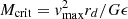 with ϵ = 0.75, where vmax is the maximum circular velocity associated with each halo (Efstathiou et al. 1982). Here, the parameter ϵ ≈ 0.5 − 0.75 is calibrated in the simulations. Although more refined treatments might be implemented (see, e.g. Romeo et al. 2023), this criterion is commonly adopted in semi-analytic models: Hirschmann et al. (2012) adopted a value ϵ = 0.75, and a similar value was adopted by Fanidakis et al. (2012). In order to investigate the maximum affect of DI on the statistical evolution of AGN, we also adopted the value ϵ = 0.75. This criterion strongly suppresses the probability for disk instabilities to occur not only in massive gas-poor galaxies, but also in dwarf galaxies that are characterized by low values of the gas-to-DM mass ratios. The instabilities induce loss of angular momentum, which results in strong inflows that we computed following the description in Hopkins & Quataert (2011), recast and extended as in Menci et al. (2014).
The BH accretion rates associated with the two feeding modes above yield an AGN emission with a bolometric luminosity LAGN = η ṀBH c2, where we assumed the accretion efficiency to take the value η = 0.1 (Yu & Tremaine 2002; Marconi et al. 2004; Shankar et al. 2020a,b). The radiation field of the AGN pushes the cold gas disk outward, determining the expansion of a shock front (Silk & Rees 1998; Cavaliere et al. 2002; King 2003; Lapi et al. 2005; Granato et al. 2004; Silk & Nusser 2010; King et al. 2011; Zubovas & King 2012; Faucher-Giguere & Quataert 2012; King & Pounds 2015). This results in the expulsion of a fraction of disk gas (AGN feedback), which is also described in the model. However, we substantially upgraded this description, as shown in detail in the next subsection.
This model was upgraded in two fundamental respects: First, the AGN feedback is now described on the basis of a complete two-dimensional model that describes the expansion of the blast wave associated with the outflow in a disk geometry, and the outflow mass is computed from this model by integrating the mass outflow rate over the directions where the outflows escape from the galactic disk. Second, we implemented a description of the bulge size and of the velocity dispersion of stars in the bulge. We describe the two upgrades in turn.
2.1. Implementing a two-dimensional physical description of outflows in galactic disks
In a previous paper (Menci et al. 2019), we provided a compact two-dimensional description for the expansion of AGN-driven shocks in realistic galactic disks with exponential gas density profiles in a disk geometry. The gas distribution was assumed to be axisymmetric (with the X-axis aligned with the plane of the disk and the Y coordinate aligned with the rotation axis), with a density profile ρ(r) = ρ0 exp(−r/rd) depending only on the galactocentric distance r and on the scale length rd, but with a cutoff in the Y direction at a distance corresponding to the disk scale height h, that is, ρ = 0 for Y ≥ h. The normalization ρ0 was such as to obtain the disk gas mass Mgas when integrated out to large radii (i.e. r → ∞), while the scale height was assumed to be constant with radius for a given galaxy and to increase with the galaxy circular velocity according to the observed average relation h = 0.45 (Vc/100 km s−1 −0.14 kpc (see van der Kruit & Freeman 2011 and references therein). Details are given in Menci et al. (2019).
The description accounts for the balance between the pressure term (fueling the expansion) that acts on the surface element corresponding to the solid angle in the considered direction and the counteracting gravitational term that is determined by the total mass M (contributed by the DM and by the central BH) within the shock radius. It includes the cooling of both the shell and gas inside the bubble due to the relevant atomic processes (inverse Compton and free-free emission; see Richings & Faucher-Giguere 2018).
We derived solutions for the outflow velocity VS, θ, the mass outflow rate ṀS,θ, and the shock position RS, θ as a function of time in different directions defined by the angle θ with respect to the plane of the disk. These depend on three fundamental quantities related to host galaxy: the AGN bolometric luminosity LAGN (fueling the expansion), the mass of cold gas in the disk Mgas (the mass that is pushed by the wind), and the total circular velocity Vc (determining the depth of the potential wells that counteract the expansion).
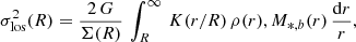
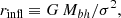
The solutions are plotted in Fig. 1 for a reference galaxy with a DM mass Mh = 1012 M⊙, a gas mass Mgas = 1010 M⊙, and an AGN bolometric luminosity L = 1045 erg s−1. The X coordinate represents the distance from the center in the direction parallel to the plane of the disk, while the Y coordinate corresponds to the distance in the (vertical) direction perpendicular to the disk.
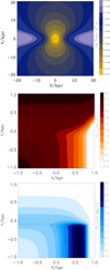 |
Fig. 1. Properties of shock expansion for our reference galaxy. In the top panel we show the positions of the shock at the different times represented by different colors and displayed in the right bar. The central and bottom panels show the velocity map and mass outflow rate map, respectively. The values corresponding to the colored contours are displayed in the bars. The X and Y coordinates correspond to the distance from the galaxy center in the directions parallel and perpendicular to the plane of the disk, respectively. |
The shock expansion radius follows the paths of least resistance (see the left panel of Fig. 1), yielding an elongated shock front in the vertical direction. Inspection of Fig. 1 shows that while in the direction perpendicular to the disk, the outflows reaches a distance of 20 kpc in approximately 107 yr, it takes about 108 yrs to reach the same distance in the plane of the disk. This has important implications for studies of AGN feedback in galaxy formation models. or an AGN life time ∼108 yrs, for instance, this would result in null gas expulsion along the plane of the disk.
Along the plane of the disk, the velocity VS, θ rapidly decreases with increasing radius (central panel), while in the vertical direction, the shock decelerates until it reaches the disk vertical boundary h, but it rapidly accelerates afterward due to the drop in the gas density outside the disk. The opposite is true for the mass outflow rate (right panel), which instead grows appreciably only along the plane of the disk, where the higher densities allow values of ṀS,θ = 0 ∼ 103 M⊙ yr−1.
These shock quantities depend on the global properties of the host galaxy and of the central AGN. For a given set of galaxy properties (cold gas mass Mgas in the disk, circular velocity of the DM halo Vc, and AGN luminosity LAGN), the predictions of the model (mass outflow rates and outflow velocities in any direction) can be compared with observation. Menci et al. (2019) tested the model against a compilation that was new then (Fiore et al. 2017) of observed outflows in 19 galaxies with different measured gas and dynamical mass, allowing for a detailed one-by-one comparison with the model predictions. Specifically, for each observed object, the measured AGN and host galaxy properties (AGN luminosity, gas mass, and circular velocity) were used to obtain the input quantities for the model. The resulting velocity and mass outflow rates computed from the model were then compared with the observed corresponding wind properties. For each considered galaxy and at the observed outflow radii, the model yielded values of the velocity and mass outflow rates (averaged over the directions) that agreed well with the observations. The predicted densities of the shocked shell were consistent with the observed molecular emission of the outflows in the vast majority of cases. The agreement we obtained for a wide range of host galaxy gas masses (109 M⊙ ≲ Mgas ≲ 1012 M⊙) and AGN bolometric luminosities (1043 erg s−1 ≲ LAGN ≲ 1047erg s−1) provides a quantitative systematic test for the modeling of AGN-driven outflows in galactic disks. This provides a solid basis for a reliable implementation of AGN feedback in galaxy formation models.
Implementing this modeling of AGN outflows in the SAM constitutes a challenging task. Directly solving the equation for the expansion of outflows in each of the simulated galaxies generated by our SAM would be too demanding in terms of computation time. Thus, we proceeded as follows.
We considered a grid of values for the three input quantities of the outflow model. Specifically, we considered 20 equally spaced logarithmic values for the AGN luminosity in the range log (LAGN/erg s−1) = 42 − 47 for a gas mass in the range log (Mgas/M⊙) = 8 − 11.5 and for a circular velocity of the host galaxy log (Vc/100 km/s) = 0.5 − 4.
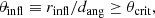
For each combination (LAGN, Mgas, Vc), we ran our model for the expansion of the outflows and computed RS, θ, VS, θ, and the mass outflow rate ṀS,θ as a function of time in different directions defined by the angle θ. We then computed the total outflow mass MS by integrating ṀS,θ over time and over all the directions in which the outflow escapes, that is, the directions in which the velocity VS, θ accelerates after it reaches the disk boundary (see Fig. 1) to reach velocities well beyond the escape velocity from the galactic halo. This provided us with tabulated values of MS (and of the critical opening angle θc corresponding to escaping outflows) for each combination (LAGN, Mgas, Vc). The expelled gas fraction fexpell = MS/Mgas and the opening angle θc as a function of LAGN and Mgas are shown in Fig. 2 for a reference value of the circular velocity Vc = 200 km s−1.
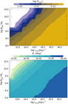 |
Fig. 2. Properties of the gas outflows. The color code shows the dependence of the fraction of cold gas that is expelled by AGN outflows (fexpell, top panel) and of the solid angle θc swept out by AGN outflows (bottom panel) on the AGN bolometric luminosity LAGN and of the cold gas mass Mcold. A DM circular velocity Vc = 200 km s−1 is assumed for both panels. |
To compute the effect of AGN feedback on each galaxy of our SAM, we interpolated these tabulated values of MS and θc to determine the escaped gas mass and opening angle corresponding to the combination (LAGN, Mgas, Vc) associated with each model galaxy in the SAM. The distribution of the average values of the expelled gas fraction fexpell as a function of the stellar mass M* and star formation rate Ṁ∗ is shown in Fig. 3.
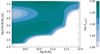 |
Fig. 3. Average fraction of gas expelled by AGN outflows in galaxies with different stellar mass M* and star formation rate Ṁ∗ shown by the color code. |
The distribution shows a bimodal shape at low values of M*. HIgh values of fexpell require either low values of Mgas (and hence low values of Ṁ∗), and/or high values of LAGN (attained for a high gas mass Mgas, yielding high values of Ṁ∗ on average). For high values of M*, the outflows can overcome the effect of the deep galaxy potential wells (yielding large expelled fractions fexpell ≈ 1) only when powered by a large AGN energy injection LAGN, which can only be attained for high values of Mgas and hence of Ṁ∗. The inclusion of a kinetically driven AGN feedback can thus trigger powerful outflows in massive galaxies that can push large portions of the gas in the intergalactic medium. This expelled gas is not reaccreted at later times. We verified that this feedback model yields stellar galaxy luminosity functions that are consistent with observations, although in this respect, the isotropic feedback model previously adopted in our SAM performed equally well.
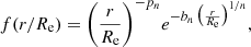
We verified that the new treatment of AGN feedback described above yields AGN luminosity functions that are consistent with existing observations. This is shown in Fig. 4, where the predicted AGN bolometric luminosity function is compared with the compilation by Shen et al. (2020) in different redshift bins extending up to z = 6. The slight overprediction at z ≳ 3 is expected. The predicted luminosity functions include Compton-thick AGN, which constitute a relevant fraction of the AGN population, with an appreciable uncertainty range ∼20 − 50% at z ≳ 3 (Shen et al. 2020), which is consistent with the slight overestimate of the observed abundance in the same redshift range. In addition, large observational uncertainties still affect the measurement of the faint end of the AGN luminosity function at z ≳ 3 (see, e.g., Shankar & Mathur 2007; Ricci et al. 2017; Shen et al. 2020). Based on results by recent surveys, the number of quasars at redshifts z ≳ 3 is being constantly revised upward. Several authors have obtained abundances of low-luminosity AGN that are up to 40 % higher than the estimates reported in the analysis by Shen et al. (2020) at both faint (MUV ≈ −23.5, Boutsia et al. 2018; Giallongo et al. 2019) and bright (MUV ≈ −27, Boutsia et al. 2021; Grazian et al. 2020) magnitudes.
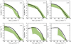 |
Fig. 4. Predicted AGN bolometric luminosity functions (solid lines) are compared to the compilation of data in Shen et al. (2020, shaded regions) in six redshifts bins shown in the labels. |
After we tested the new treatment of AGN feedback in the SAM, the AGN luminosity functions were consistent with existing observations over a wide range of redshift. We then proceeded with the extension of the SAM to include a description of the stellar velocity dispersion, as detailed below.
2.2. Computing Jeans-based stellar velocity dispersions
We here further extended our SAM with respect to previous renditions of the model to include the most recent calculations of the half-mass radii and stellar velocity dispersions. The former were presented in Zanisi et al. (2020). Half-mass galactic radii in progenitor disks are computed from angular momentum conservation with the host halo spin. When galaxies merge, a stellar bulge is formed with the half-mass radius Rh, which is computed via energy conservation between the gravitational potential energies of the progenitors and the descendant (e.g., Cole et al. 2000). We tested that the sizes computed in our SAM match the observed correlation with stellar mass for the redshift range covered by observations for star-forming and quiescent galaxies. To perform the comparison, we adopted the approach in Shankar et al. (2014). Assuming that light traces mass, the above authors converted Rh into projected half-light radii Re using the tabulated factors from Prugniel & Simien (1997), that is, Re ≈ 2S(n) Rh, with the scaling factors S(n) dependent on the Sérsic index n. Following Shankar et al. (2014), for we adopted a fixed value n = 4 for this. As noted by the above authors, while it is possible to predict a Sérsic index a priori from the models in principle (e.g., Hopkins et al. 2009), this relies on several additional assumptions on the exact profile and the evolution with time of the dissipational and dissipationless components, so that the true advantage with respect to simply empirically assigning a constant Sérsic index is modest. By the same token, we note that none of our main results would change if we were to assign stellar mass-dependent Sérsic indices and/or effective radii directly extracted from the observed distributions to our mock galaxies.
The predicted correlation between the size Re and the stellar mass is compared with observations in Fig. 5 for different redshift bins and for both quiescent and star-forming galaxies. Following the approach in Genel et al. (2018), we classified our SAM-generated galaxies as early- or late-type through their specific star formation SSFR = Ṁ∗/M∗. Galaxies are defined as quenched when their SSFR is at least 1 dex below the ridge of the star formation main sequence. This is defined, for simplicity, as log(SSFR/Gyr−1) = − 0.94, −0.85, −0.35, and 0.05 for z = 0, 0.1, 1, and 2, respectively. On the observational side, van der Wel et al. (2014) classified early- and late-type galaxies on the basis of their star formation properties, defined in terms of cuts in the (U–V)–(V–J) rest-frame colors, while Bernardi et al. (2014) adopted a morphological classification based on a Bayesian automated procedure. We assumed that our model half-light radius Re was computed assuming that light traces mass. On the other hand, the different observations are made in different bands. While the measurements of Bernardi et al. (2014) were performed directly in the Sloan Digital Sky Survey (SDSS) r band, those from van der Wel et al. (2014) were made in the Hubble Space Telescope Wide Field Camera 3 (WFC3) F125W filter, which is centered on an observed frame wavelength of 1.25 μm. In order to match the SDSS-based studies, we converted the measurements in van der Wel et al. (2014) into the SDSS r band using the gradient d log Re/dlogλ that they directly measured between the F814W (814 nm) and F125W filters.
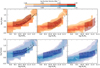 |
Fig. 5. Predicted distribution of the effective radius Re shown as a function of the stellar mass M* at redshifts z = 0.25, z = 1.51, and z = 2.25 (from left to right) for early-type (top row) and late-type galaxies (bottom row). The predictions are compared with the data from van der Wel et al. (2014; shaded areas). We also show the size-stellar mass relation measured at z = 0.1 by Bernardi et al. (2014) and Mowla et al. (2019) as dashed lines and dots, respectively. |
From the galaxy size computed as shown above, we derived the corresponding velocity dispersion by solving the spherical Jeans equation, following Desmond & Wechsler (2017). For the bulge component, this reads
 (1)
(1)
where  is the orbit anisotropy profile relating the radial velocity dispersion σr to the tangential component σθ, ρ(r) is the mass density profile of the bulge, and M*, b is the bulge stellar mass.
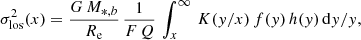
The line-of-sight velocity dispersion solving Eq. (1) is then given by Mamon & Łokas (2005; see also Desmond & Wechsler 2017) in the form
 (2)
(2)
where R is the projected distance from the center, and Σ(R) is the projected density profile. The function K is defined as a combination of gamma functions Γ and incomplete β functions B,
 (3)
(3)
![Mathematical equation: $$ \begin{aligned}&\qquad +\beta B(1/u^{2},\beta +1/2,1/2)-B(1/u^{2},\beta -1/2,1/2)] ,\end{aligned} $$](/articles/aa/full_html/2023/06/aa44574-22/aa44574-22-eq10.gif) (4)
(4)
where u ≡ r/R, and β is the assumed orbit anisotropy.
For each model galaxy, we assumed for Σ(R) a Sersic form Σ(R) = Σ0 g(R) with
![Mathematical equation: $$ \begin{aligned} g(R/R_{\rm e})=e^{ {-b_n\, \big [ \big ( {R\over R_{\rm e}} \big )^{1/n}-1 \big ]} }, \end{aligned} $$](/articles/aa/full_html/2023/06/aa44574-22/aa44574-22-eq11.gif) (5)
(5)
where bn ≈ 2n − 1/3 + 0.009876/n. This was normalized to yield the bulge mass M*, b when integrated over R, so that 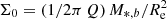 , where
 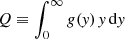 .
.
The corresponding deprojected mass density profile is ρ(r) = ρ0 f(r/Re), where
 (6)
(6)
where pn = 1 − 0.6097/n + 0.00563/n2. Again, the normalization ρ0 was computed so as to obtain the total mass M*, b when the above mass density profile was integrated over the volume. Thus, 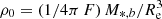 , where
 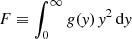 .
.
Finally, the bulge mass density profile is 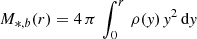 . Inserting the above form for the density profile ρ(r), we obtain
 (7)
(7)
Inserting Eqs. (4)–(6) in Eq. (2), we obtain
 (8)
(8)
where x ≡ R/Re.
In the following, we consider the average velocity dispersion
 (9)
(9)
When a finite-aperture radius Rap is considered, the upper limits in the above integrals should be replaced with xap ≡ Rap/Re. Inserting the expression in Eq. (7), we obtain
 (10)
(10)
with the shape factor W defined as
 (11)
(11)
The velocity dispersion is thus related to the virial value GM*, b/Re through the shape factor W(β, n), which depends on the structural properties of the bulge (anisotropy parameter β and Sérsic index n).
For each simulated galaxy in our SAM, the effective bulge mass content M*, b and radius Re allowed us to derive the average bulge velocity dispersion from Eqs. (10) and (11) for a given choice of β and n. For the first, we extracted a random value from a Gaussian distribution with an average value ⟨β⟩ = 0.3 and dispersion 0.35. This choice has been shown to provide a good fit to observational data (Desmond & Wechsler 2017). For the Sérsic index n, we adopted a fixed vale n = 4 based on the considerations presented above. To test that the treatment above was consistent with available data, we compared (Fig. 6) the velocity dispersion of passive model galaxies (Ṁ∗/M∗ ≤ 0.1 Gyr−1) at low redhsift (z ≤ 0.1) to existing data for early-type galaxies in the SDSS database (Bernardi et al. 2011), selected on the basis of morphological indicators (Hyde & Bernardi 2009). The observational correlation does not change appreciably when passive galaxies are selected on the basis of spectral or color indicators (Belli et al. 2014; Zahid et al. 2016). These galaxies are characterized by high bulge-to-disk stellar mass ratios B/T ≳ 0.8, for which the total galaxy velocity dispersion is dominated by the bulge component computed in Eq. (8)–(11). For consistency with the data by Hyde & Bernardi (2009), we adopted xap = 1/8 when computing Eq. (8), (this leads to a small offset −0.03 in log(σ) when compared to the global average corresponding to xap → ∞). The excellent agreement shown in Fig. 6 provides a reliable basis for computing the scaling relations between the BHs and the properties of the host galaxies, as well as for including the effects of observational selection biases in the analysis of model results, as we discuss below.
 |
Fig. 6. Predicted relation between the velocity dispersion σ and the stellar mass M* for passive galaxies (see text). The color code represents the logarithm of the fraction of model galaxies with the considered σ for each bin of M*. The shaded band shows the relation for early-type galaxies selected on the basis of morphological indicators after Hyde & Bernardi (2009). The dashed black and red lines show the average relation derived by Zahid et al. (2016) for passive SDSS galaxies and for the Smithsonian Hectospec Lensing Survey (SHELS) sample, selected on the basis of spectral properties (Dn4000 > 1.5, where Dn4000 is the flux ratio of two spectral windows adjacent to the 4000 Å break (see Balogh et al. 1999). |
3. Selection bias
Shankar et al. (2016) showed that a selection bias may affect the observe scaling relations when dynamical measurements of the BH mass are considered. These mass estimates are only possible when the sphere of influence of the BH,
 (12)
(12)
has been resolved in the observations (e.g., Peebles 1972; Gültekin et al. 2011; Graham & Scott 2013).
This means that the observed correlations between dynamically measured BH masses and the galaxy properties automatically select objects for which
 (13)
(13)
where dang is the angular distance of the object, and θcrit is the resolution limit of the instrument (e.g., θcrit ≈ 0.1 for observations with the Hubble Space Telescope, HST).
Shankar et al. (2016) estimated the impact of this observational bias on the comparison between the predicted and the observed scaling relations under different assumptions on the intrinsic scaling relations.
Our improved semi-analytic model allowed us to investigate the impact of this observational bias on the basis of the ab initio model for galaxy formation presented in the previous section, tested against a wide number of observations. Our computation of the velocity dispersion σ in terms of the properties of the host galaxy enables the prediction of the BH sphere of influence rinf for each simulated galaxy of our model.
In the following, we exploit the model predictions of rinf to investigate the impact of the selection bias affecting the dynamical BH mass measurements on the comparison between the predicted and the observed BH scaling relations.
4. Results
Before performing a detailed comparison of our predictions for the BH scaling relations with available data, we first show the effects of the model improvements presented in the previous section, that is, the inclusion of the two-dimensional angle-dependent AGN feedback model presented in Sect. 2.1 and the σ dependent selection bias described in Sect. 3. With this aim, we compare in Fig. 7 the MBH − M*, b relation that we obtained by adopting our two-dimensional feedback model (upper panels) with that obtained using the isotropic AGN feedback model previously adopted in our SAM (lower panels). To show the effect of the selection bias, the results from models including the bias (right columns) are compared to those without this effect (left columns).
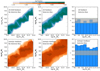 |
Fig. 7. Effect of feedback treatment on the MBH − M*, b relation. The relation predicted for galaxies at z ≤ 0.1 by our new two-dimensional model for AGN feedback (top panels) presented in Sect. 2.1 is compared with the predictions obtained with our previous isotropic treatment of feedback (bottom panels). For both AGN feedback models, we show the results with and without the selection effect discussed in Sect. 2.1, as indicated by the labels. In all panels, the color code corresponds to the logarithm of the fraction of galaxies with different MBH in a given log M*, b bin. The standard deviations ϵ for the new and previous treatment of AGN feedback is shown as a function of bulge stellar mass in the rightmost histograms. The horizontal strip represents the range of values obtained from different observational works: the upper bound is the intrinsic scatter ϵ derived by De Nicola et al. (2019), and the lower bound is the value of ϵ derived by the least-square fit analysis by Kormendy & Ho (2013) using individual errors in log σ, adding individual errors in log MBH to the intrinsic scatter in quadrature, and iterating the intrinsic scatter until the reduced χ2 = 1. |
The comparison between the first and the second column in Fig. 7 shows that a true relation between the BH mass MBH and the bulge mass is indeed expected in the isotropic and in the two-dimensional, angle-dependent AGN feedback models, regardless of whether the selection effect resolution of the BH sphere of influence is considered. The main effect of including the selection bias is that the distribution of the model galaxies is extended toward higher BH masses (especially for high M*, b), which agrees better with the observations.
It is interesting to note that the slope of the scaling relations in the case of two-dimensional, angle-dependent AGN feedback is almost unchanged for an isotropic AGN feedback. We therefore conclude that the detailed form of AGN feedback is not the main cause for the scaling relations, which instead appear mostly to be driven in our model by the dependence of the BH mass on the processes connected to the growth of the stellar content and of the host galaxy, which in turn imply a correlation between MBH and σ. Interestingly, Marsden et al. (2022) have recently shown that a steep and nearly constant MBH − σ relation naturally arises from the coupling of the observed LX − M* relation and a Jeans-based stellar velocity dispersion (similarly to what we carried out here), without any additional fine-tuning.
However, the adoption of the two-dimensional, angle-dependent description of AGN feedback has an important effect on the scatter of the relations, as shown quantitatively in the rightmost panels of Fig. 7. The adoption of our new two-dimensional model for AGN feedback reduces the intrinsic scatter from values ϵ ≲ 0.5 − 0.6 (obtained in the isotropic feedback case) to values ϵ ≲ 0.3. This is due to the following reasons: In the new two-dimensional model for feedback, the blast wave expansions stalls along the direction of the disk, and the radius within which the expansion stops strongly depends on the gas density of the disk and the AGN luminosity. This means that the opening angle (and hence the fraction of expelled gas) is larger when the gas density is low (because less energy has to be spent to push the gas outward) and when the AGN luminosity is high (because more energy is available to push the blast wave outward), as shown in Fig. 2. Both quantities depend on the merging histories and are related because the AGN luminosity LAGN depends on the available cold gas reservoir Mgas. The high efficiency of feedback in galaxies with particularly low Mgas (for a given LAGN) or in those with particularly large LAGN (for a given Mgas) inhibits the BH growth in all the host galaxies that are outliers with respect to the average relation between Mgas and LAGN. This results in a smaller scatter.
The MBH − M*, b relation predicted by our improved model is compared with the data in Fig. 8. The observational data with which we compared the relation include BH estimates for both quiescent and active BHs.
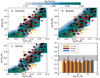 |
Fig. 8. Comparison of our predicted MBH − M*, b relation with the data for all galaxies at z ≤ 0.1. The color code corresponds to the logarithm of the fraction of galaxies with different MBH in a given log M*, b bin. Panel A: Predicted relation between the BH mass MBH and the bulge stellar mass M*, b. The data points are from Kormendy & Ho (2013; black squares and triangles for elliptical galaxies and bulges, respectively), Savorgnan & Graham (2016; red dots), and Ho & Kim (2014; orange filled squares). Panel B: Same as panel A, but including the selection bias discussed in Sect. 3, i.e., considering only model galaxies satisfying the condition in Eq. (12) with θcrit = 0.1. Panel C: Same as panel A, but considering only model galaxies hosting AGN with bolometric luminosity LAGN ≥ 1044 erg s−1. Bottom right panel: Rms value of the scatter of the distributions shown in panel A (brown histogram), panel B (blue histogram), and panel C (orange histogram) for different bins of M*, b. The horizontal strip corresponds to the range of measured intrinsic scatter by different authors. The lower value ϵ = 0.28 was obtained by Kormendy & Ho (2013) and the upper value ϵ = 0.4 was obtained by Savorgnan et al. (2016). |
First, we considered the BH mass measurements collected from spatially resolved estimates available from the literature for bulges or bulge-dominated galaxies, that is, the data set including bulges and elliptical galaxies in Kormendy & Ho (2013), and the extended data sets in Savorgnan & Graham (2016) and De Nicola et al. (2019). The first data set consists of 66 galaxies with dynamical estimates of their black hole masses as reported by Graham & Scott (2013) or Rusli et al. (2013). Using 3.6 μm (Spitzer satellite) images, Savorgnan & Graham (2016) modeled the one-dimensional surface brightness profile of each of the 66 considered galaxies and estimated the structural parameters of their spheroidal component by simultaneously fitting a Sérsic function. Following Shankar et al. (2016), we retained only the galaxies with secure black hole mass measurements from the original Savorgnan & Graham (2016) sample and removed the sources that wer eclassified as ongoing mergers. This limited the final sample to 48 galaxies, 37 of which are early-type galaxies (ellipticals or lenticulars) that we considered in our comparison. De Nicola et al. (2019) derived a sample of 83 galaxies based on the compilation of Saglia et al. (2016) whose BH masses were derived from spatially resolved kinematics.
We also compared our predicted MBH − M*, b relation with the observed relation for active galaxies whose BH masses were derived from the (presumed) virial motions of the broad line region (BLR) gas cloud orbiting in the vicinity of the central compact object: MBH = fvir r(ΔV)2/G. Here, r is the radius of the BLR, which is derived from reverberation mapping (e.g., Blandford & McKee 1982; Peterson 1993), or reverberation-based methods that use the radius-luminosity relation (e.g., Bentz et al. 2006). The characteristic velocity ΔV was derived from the width of the emission lines (a common line is Hβ). As motions in the BLR are not perfectly Keplerian, the parameter fvir is included in the equation to account for the uncertainties in kinematics, geometry, and inclination of the clouds. This was calibrated by comparing reverberation-mapped AGNs with measured bulge stellar velocity dispersions against the MBH − σ relation of inactive galaxies. We considered the compilation by Ho & Kim (2014), who derived a virial coefficient fvir = 6.3 ± 1.5 for classical bulges and ellipticals.
The treatment of the AGN feedback we adopted in our semi-analytic model yields BH scaling relations that match the observations when the observational bias related to the resolution of the BH sphere of influence is considered. Again, the inclusion of this bias extends the distribution of model galaxies toward higher BH masses (especially for high M*, b), which agrees better with the observations. Shankar et al. (2016) discussed that the degree of the impact of the bias between the normalization of the intrinsic and observed BH-galaxy scaling relations depends on the type of the intrinsic relation that is considered. Assuming an intrinsic relation scaling MBH ∝ σα with α ≳ 4 would lead to a jump between intrinsic and observed relations that is larger than assuming, for example,  with β ≈ 1 as the intrinsic relation. Our current SAM predicts an average difference of ≲2 between intrinsic and observed scaling relations, which is what would be expected if the BH mass depends more weakly on the velocity dispersion and/or is more strongly correlated with stellar mass than with the velocity dispersion (models 2 and 3 in Shankar et al. 2016), as also highlighted in the residuals below.
We also note that the predicted distribution of model galaxies with an active AGN (LAGN ≥ 1044 erg s−1) does not appear to differ substantially from the distribution of the whole population. However, some of the observational points related to active galaxies lie out of the strip representing the model predictions. While a possible explanation is that some of the outflows in these galaxies are spherical, it is possible that the apparent discrepancy in the normalizations of the MBH − M*, b scaling relations characterizing local AGN data and local inactive BH samples with dynamical mass measurement is due to the presence of some additional biases in the BH and/or the stellar mass estimates between the two BH samples, so that the AGN data represent a biased sample of the whole population (see, e.g., Shankar et al. 2019; Farrah et al. 2023, and references therein). We further investigate this point below.
The scatter we obtain agrees well with the observations, for which most observations yield values in the range 0.3 ≲ ϵ ≲ 0.4 (see the references in the caption), although some authors find somewhat higher values (see Sahu et al. 2019a,b). Tehe novel treatment of AGN feedback we considerd reduces the scatter of these relations with respect to the adoption of an isotropic average feedback. This is shown in Fig. 9, where we compare the MBH − M*, b relation (including the selection bias described in Sect. 3) obtained with the two-dimensional model presented in Sect. 2.1 with our previous isotropic treatment of AGN feedback described in Menci et al. (2014).
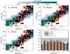 |
Fig. 9. Comparison of our predicted MBH − σ relation with data for all galaxies at z ≤ 0.1. The color code corresponds to the logarithm of the fraction of galaxies with different MBH in a given log σ bin. Panel A: Predicted relation between the BH mass MBH and the bulge velocity dispersion σ brightness-weighted averaged over the galaxy. The data points are from Kormendy & Ho (2013; black squares and triangles for elliptical galaxies and bulges, respectively), De Nicola et al. (2019; brown squares), Savorgnan & Graham (2016; red dots), and Ho & Kim (2014; orange filled squares). Panel B: Same as panel A, but including in the model the selection bias discussed in Sect. 3, i.e., considering only model galaxies that satisfy the condition in Eq. (12) with θcrit = 0.1. Panel C: Same as panel A, but considering only model galaxies hosting AGN with bolometric luminosity LAGN ≥ 1044 erg/s. Bottom right panel: Histograms represent the rms values of the scatter for the distributions shown in the top left (brown), top right (blue), and bottom left panel (orange). The horizontal strip represents the range of values obtained from different observational works: the upper bound is the intrinsic scatter ϵ derived by De Nicola et al. (2019), and the lower bound is the value of ϵ derived by the least-square fit analysis by Kormendy & Ho (2013) using individual errors in log σ, adding individual errors in log MBH to the intrinsic scatter in quadrature, and iterating the intrinsic scatter until the reduced χ2 = 1. |
We present in Fig. 9 the predicted relation between BH mass MBH and the bulge velocity dispersion σ for galaxies at z ≤ 0.1. In addition to the intrinsic relation, we also show the relations that we predict when the selection bias presented in the previous section is considered (i.e., for model galaxies that satisfy condition in Eq. (12)) and when only active galaxies (i.e., galaxies hosting an AGN with luminosity Lbol ≥ 1044 erg s−1) are considered. Although in the plot, σ refers to the bulge velocity dispersion, we verified that for galaxies with B/T ≥ 0.3, the model predictions do not change substantially when the global σ is computed from the total galaxy size and total stellar mass M* (in this case, we used a stellar mass dependent Sérsic index as given in Terzic & Graham 2005).
In the comparison, we assumed that stellar mass traces light because the mass-weighted averaged velocity dispersion in Eq. (8) derived for model galaxies is compared with observed values derived from a brightness-weighted average (see, e.g., De Nicola et al. 2019).
The comparison between the observational data and the model predictions provides interesting insight on some crucial points.
– The comparison between panels A and B shows that a true relation between the BH mass MBH and the bulge mass is indeed expected, regardless of the inclusion of selection effects. In the model, the observed correlation does not consist of the upper envelope of the scatter of a distribution of BH masses that extends to lower BH masses, as suggested by some authors (see, e.g., Batcheldor 2010), which is also in line with the findings by Shankar et al. (2016).
– However, when we compare the results in panels A and B, the distribution of the model galaxies in the MBH − σ plane agrees better with the observational data when the selection effect discussed in Sect. 3 is considered. When this bias is included, the distribution of the model galaxies extends toward higher BH masses, which agrees better with observations. However, this extension is less pronounced than the extension that affects the predicted MBH − M*, b relation. This effect has been noticed by Shankar et al. (2016) and led these authors to conclude that this suggests that the MBH − σ relation is the true fundamental relation, while the MBH − M*, b relation is mostly a consequence of the MBH − σ and σ − M*, b relation. We investigate this point in detail below.
– When the selection bias is considered, not only the bulk of the population of model galaxies is consistent the observed relation, but the scatter in the distribution also agrees excellently with the distribution of data points.
– It is extremely interesting to note that the SAM predicts a MBH − σ relation of similar normalization and dispersion with respect to the collection of available data sets in the local Universe, but with a flatter slope. The predicted MBH − σ relation has a slope of ∼2.5 when selection effects are included (panel B), and somewhat lower x (∼2.2) in the intrinsic relation. This result is in line with what has been suggested in other theoretical and numerical works. Cavaliere & Vittorini (2002; see also Vittorini et al. 2005) highlighted the fact that if the quasar-feedback condition (e.g., Silk & Rees 1998; King 2003) is not constantly applied throughout the evolution of BHs, the resulting MBH − σ relation would have a slope closer to ∼3 rather than 4 − 5. This also agrees with some recent (Caglar et al. 2023) and previous (Woo et al. 2013, Park et al. 2012a) observational findings. On the numerical side, Li et al. (2020) recently showed that the TNG100 simulation also produces a MBH − σ relation with a slope of ∼3 (their Fig. 1, bottom panels) that is in general above the data, where the latter effect could also at least in part be ascribed to selection effects in the local observational data sets (e.g., Shankar et al. 2016, Li et al. 2020). Sijacki et al. (2015) and Thomas et al. (2019) found in the Illustris and SIMBA simulations, respectively, a slope and normalization for the MBH − σ relation that is consistent with observations. However, a MBH ∝ σα, with α ≳ 4 − 5, in some simulations/models might also in part be an artifact of a steeper M* − σ relation in the same models, as discussed in Barausse et al. (2017), as in the case of the Horizon-AGN simulation (Dubois et al. 2016).
– Analogously to what we predict for the MBH − M*, b relation, the predicted distribution of model galaxies with an active AGN (LAGN ≥ 1044 erg s−1) does not seem to differ substantially from the distribution of the whole population.
In summary, the predicted distribution of galaxies in the MBH − σ plane covers the regions allowed by available data. However, our SAM, in line with some other current models discussed above, does not fully match the steep slope of the MBH − σ relation, as inferred from current local data. This might be interpreted in two ways: (1) either the local sample is incomplete, and/or (2) current cosmological models for the coevolution of BHs and galaxies are still missing some ingredients, either in the AGN feedback process itself and/or in other events during the growth of the BH (e.g., Cavaliere et al. 2002). In our model, the only viable way to increase the slope in the MBH − σ relation would be to slightly increase the anisotropy parameter with stellar mass from 0.3 to 0.35, but this would also steepen the σ − M* relation, which would worsen the match with observations. A trade-off between the inclusion of the dark matter component and stellar anisotropy might improve the fit to both observables simultaneously. The main lesson we learn from previous studies and the one conducted in this work is that at face value, AGN kinetic feedback by itself may not be sufficient to entirely reproduce the current observational data on local BHs. This is further corroborated by the analysis of the residuals that we present below.
To go beyond the study of pairwise correlations between MBH, M*, b and σ and gain better insight into the joint distribution of these quantities, we now focus on our predictions for the residuals of the BH-galaxy scaling relations. For any pair of quantities X and Y, these are defined as Δ(Y|X)≡log Y − ⟨log Y|log X⟩. As proposed by various authors (see, e.g., Shankar et al. 2016), the correlations between the residuals provide additional information about the joint distribution of MBH, σ and M*, and can provide a way of determining which variable is more important in determining the MBH − M* and MBH − σ relations. In the ideal case where MBH was fundamentally determined by σ alone, for instance, the residuals from correlations with σ would be uncorrelated, while residuals from the MBH − M* relation would correlate with residuals from the σ − M* relation.
In the left and the right panels of Fig. 10 we show Δ(MBH|M*) vs Δ(σ|M*) and Δ(MBH|σ) versus Δ(M*|σ) predicted for bulge-dominated model galaxies (B/T ratio ≥0.8), and compare these relations with those derived for the sample of Savorgnan et al. (2016) of early-type galaxies, for which residuals were computed in Shankar et al. (2016) and Barausse et al. (2017).
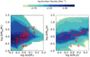 |
Fig. 10. Predictions for the residuals of the BH-galaxy scaling relations. In the left panel, we show the correlation between the residuals of the MBH − M*, b relations and those of the σ − M* relation at fixed stellar mass. The correlation between the residuals of the MBH − σ relation and those of the M* − σ relation at fixed velocity dispersion are shown in the right panel. Data points refer to the sample of Savorgnan et al. (2016). The contours refer to model galaxies with a bulge-to-total stellar mass ratio B/T > 0.8 for which the black hole sphere of influence can be resolved. |
The predicted residuals occupy the same regions as the observational data points, showing that the model captures the complex intertwining between the considered quantities. As expected, the predicted behavior of the residuals is complex, and none of the considered quantities can be considered as really fundamental in our SAM. In the framework of cosmological galaxy evolution models such as our SAM, the BH mass stems from the complex interplay between the growth history of the halo mass and the physics of baryons, which cannot be easily reduced to a single fundamental dependence on a single quantity.
Testing the consistency of this picture with existing data is not straightforward because the model does not provide definite correlations between the residuals, but rather distributions in the Δ(MBH|M*)−Δ(σ|M*) and Δ(MBH|σ)−Δ(M*|σ|) planes. Thus, we performed a two-dimensional Komlogorov-Smirnov (KS) test to assess the consistency of the predicted distributions with the observational points. To do this, we followed the approach in Fasan & Franceschini (1987) using the extended two-dimensional KS distance D defined in Peacock (1983). We ran a Monte Carlo simulation to generate synthetic data sets from the predicted distributions, each set with the same number of points Ndata as the real data set. For each Monte Carlo realization, we also generated Ndata observational data points distributed according to the measured data points and error bars. We then computed D for each synthetic data set using the approach mentioned above and counted the fraction of the time for which these synthetic Ds exceeded the D from the real data. The resulting fraction provides the significance level QKS for the consistency between the data distribution and the model distribution. For the Δ(MBH|σ)−Δ(M*|σ|) relation, we obtain a significance level QKS = 0.24, indicating that the former data distribution is compatible with the model predictions. For Δ(MBH|M*)−Δ(σ|M*), we obtain QKS = 0.1. This value leaves open the possibility that either the sample of local BHs is still incomplete and/or that some element is still missing in the cosmological models that generates the dependence between MBH and σ (see also the results by Barausse et al. 2017, who claimed the absence of the correlation Δ(MBH|M*) and Δ(σ|M*) in both hydrodynamic simulations and SAMs).
In this context, we expect BH masses to be correlated with different DM and baryonic properties of galaxies, all emerging from the above complex interplay. To investigate this point in closer detail, we computed the relation between the BH mass and the global properties of galaxies, such as the total stellar mass content and the DM mass. We stress that these relations are expected in all cosmological models of galaxy formation because all baryonic processes (gas cooling and accretion, inflows, star formation, and feedback) are ultimately related to the depth and growth history of the gravitational potential wells. In this framework, the growth of the stellar, BH, and DM components are intertwined so that MBH, M*, and Mh are expected to be related to each other. The connection among these quantities is investigated in Fig. 11 and is compared with recent observational measurements by Marasco et al. (2021). These authors identified a sample of 55 nearby galaxies with dynamically measured MBH ≥ 106 M⊙ for which dynamical measurements of Mh were available, based either on globular cluster dynamics (for galaxies of earlier Hubble types) or on spatially resolved rotation curves (for galaxies of later Hubble types). The correlation we find between the BH mass MBH and the total stellar mass content M* agrees excellently with observations in both strengths and scatter, the latter being characterized by an intrinsic value ϵ ≈ 0.45. As expected, we find an extremely well-defined correlation between MBH and Mh, in agreement with the results in Marasco et al. (2021) and with previous authors (Ferrarese 2002; Pizzella et al. 2005; Volonteri et al. 2011; Davis et al. 2019a,b; Shankar et al. 2020a,b; Smith et al. 2021) who used the vrot as a proxy for the DM mass Mh. Although our model includes the merging of BHs as a key process, our predicted MBH − M* relation does not show any sign of flattening at high masses. This feature has been suggested to be indicative of merging events as the leading process in the building up of the relation for early-type massive galaxies (see Graham & Sahu 2023). This suggest that the gas physics is relevant in the build-up of the relation even for massive galaxies.
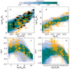 |
Fig. 11. Predicted relations between MBH and the stellar and DM properties of the host galaxies. The MBH − M* relation (panel A), the MBH − Mh relation (panel B), the f* − MBH relation (panel C), and the f* − Mh relation (panel D) are compared with the data from Marasco et al. (2021; orange points). In panel A we also report data from Sahu et al. (2019a,b; black dots). The gray contours show the predictions of our model in the absence of AGN feedback. In all panels and for each abscissa value, the color code corresponds to the logarithm of the fraction of galaxies with different values of the quantities in the y-axis. |
The tightness of the relation is directly related to the presence of AGN feedback. In a model without AGN feedback, the relation between MBH and M* is expected to be much broader, as shown by the gray contours in panel A of Fig. 11.
Thus, the observed tight correlation between MBH and M* results from the interplay between the growth of DM halos (and the ensuing collapse and cooling of gas in the DM potential wells, and the related dynamical processes affecting the distribution of gas) and the counteracting effects of AGN outflows, which keeps the relation tight.
Because all baryonic processes entering the BH growth are ultimately related to the growth of the DM halos, we expect a tight correlation between the BH mass MBH and the DM halo mass of the host MH. This is shown in panel B and is compared with data. The relations resulting from the model appear to be tighter than the data distribution. However, the large error bars of the data points currently do not allow us to validate or falsify the model prediction. Here we note that recent observations of central galaxies in galaxy clusters show an extremely tight relation between the BH and the halo mass (Gasparri et al. 2019), tighter indeed than the MBH − M* relations. This supports our prediction of a strong correlation between MBH and Mh, as found in ab initio models and cosmological simulations (see Davies et al. 2023 for recent results, and references therein).
However, as stressed by the authors above, the complex physics of baryons in the growing DM potential wells results in a number of correlations. Like all cosmological models of galaxy formation, our SAM predicts a strict relation between the depth of the gravitational potential wells and the star formation processes (panel D). In particular, the star formation efficiency f* ≡ M*/fb Mh (here fb is the Universal baryon fraction) is predicted to have a maximum for DM masses of about Mh ≈ 1012 M⊙. For lower values of Mh, star formation is suppressed by the strong effects of stellar feedback, which effectively expels a relevant fraction of gas from the shallow potential wells, while in massive halos with Mh ≳ 1012 M⊙, the inefficiency of gas cooling and strong AGN winds combine to quench star formation, leading to a declining f* (see also Shankar et al. 2006). Thus, matching the observed behavior (panel D) provides a key test for our implemented 2-dimensional AGN feedback model. It is important to stress that such a model provides a combined correlation between the quenching properties of AGN feedback (the quantity f*) and its function of self-regulation in the growth of BHs, as shown in panel C. The consistency between the predicted and the observed relation between MBH and f* provides an important consistency check for our implemented AGN feedback model because it provides a simultaneous quantitative description of both the star formation quenching and the regulation of the BH growth that is consistent with available measurements.
This correlation between the AGN feedback and the star formation properties of galaxies is expected to impact over the distribution of BHs with different degree of activity in the MBH − M* plane. This is investigated in detail in Fig. 12, where we show the MBH − M* relation for different BH Eddington ratios λ, and compare them with data for active AGNs with BH masses measured through either reverberation mapping or maser techniques (van den Bosch 2016), so that they are not affected by uncertainties related to fvir. As noted by previous authors (e.g., Reines & Volonteri 2015; Shankar et al. 2019), these objects appear to lie below the relation for the global BH population. Interestingly, although the model predicts BH masses of active galaxies somewhat higher than observed, it predicts that objects with higher Eddington ratios lie systematically along the lower envelope of the global MBH − M* relation. The physical interpretation of this trend is that extremely high accretion rates only take place in objects in which large gas reservoirs are still available and have not been converted into stars and high BH masses at higher redshifts. Although the distribution is consistent with available data, we note that a detailed verification of our prediction would require a larger collection of observational points, which would enable us to sample the distribution of Eddington ratios with sufficient statistical significance. The apparent discrepancy/offset in the normalizations of the MBH − M* scaling relations characterizing local AGN data and local inactive BH samples with dynamical mass measurements is a matter of intense debate (e.g., Reines & Volonteri 2015; Shankar et al. 2019; and references therein), and is not yet solved. Although it is beyond the scope of the current work to discuss this difference in depth, we note that the dispersion predicted by our SAM is more contained than the one observed in the combined data sets, possibly suggesting the presence of some additional biases in the BH and/or the stellar mass estimates between the two BH samples.
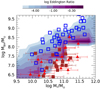 |
Fig. 12. Average Eddington ratio of BHs in the MBH − M* plane (color-coded). The blue data are taken from Savorgnan & Graham (2016), and the red squares and triangles are the data obtained from reverberation mapping and maser techniques, respectively. These are taken from van den Bosch (2016). To the error bars reported by the latter authors (referring to measurement errors in the K-band magnitude), we have added (in quadrature) a systematic error estimate of 0.3 dex corresponding to the uncertainties in the conversion from k-band magnitudes to stellar masses. |
Finally, we investigated the predictions of our updated model on the evolution of the MBH − M* relation. Specifically, we compared our results with the recent measurements at 1.2 ≤ z ≤ 1.7 based on 32 X-ray selected broad-line AGN performed by Ding et al. (2020). By applying modern tools to decompose the HST images including available ACS data, the authors measured the host galaxy stellar mass through the two-dimensional model fitting, while the BH mass was determined using the broad Hα line, detected in the near-infrared with the Subaru Fiber Multi-Object Spectrograph.
To ensure a fair comparison with these observations, we reproduced the selection biases when considering the model galaxies. Specifically, we adopted the same selection window as in the observations λEdd ≥ −0.5 − 0.11 * (log(MBH/M⊙)−7.5, based on the Eddington ratio λEdd (see Fig. 1 of Ding et al. 2020). In addition, following Ding et al. (2020), we injected random noise to the sample of model galaxies to mimic the scatter in the data due to measurement errors, that is, δMBH = 0.4 dex and δM* = 0.17 dex, so as to allow for a quantitative comparison between the observed and predicted scatter in the MBH − M* relations.
The result of the comparison is shown in Fig. 13, where we show the prediction for both the whole sample of model galaxies and for the subsample that was selected to mimic the observational measurement errors and selection effects. When the latter are considered, the distribution of model galaxies matches the observations in both central value and scatter. The former shows a small positive evolution ΔMBH ≈ 0.5 with respect to the local relation, which is consistent with results from N-body simulation (see, e.g., Sijacki et al. 2015; Khandai et al. 2015; De Graf et al. 2015). On the other hand, the scatter takes values ranging from ϵ ≈ 0.3 to ϵ ≈ 0.38, which excellently agrees with the observed value ϵ ≈ 0.35.
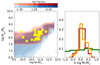 |
Fig. 13. Model predictions for the evolution of the MBH − M* relation. Left panel: comparison of the observed (orange dots) and predicted MBH − M* relation for galaxies in the redshift range 1.2 ≤ z ≤ 1.7. The color code corresponds to the logarithm of the fraction of galaxies with different MBH in a given log M* bin. The data are taken from Ding et al. (2020). The total predicted distribution of model galaxies in the MBH − M* plane is shown by the blue contours, and the red region corresponds to the subsample of model galaxies that satisfies the same selection criteria as the observations. Right panel: distribution of the residuals for the observations (orange histogram), the model galaxies (blue histogram), and the model galaxies resulting in simulations with the isotropic feedback model implemented in previous versions of our SAM (green histogram, taken from Ding et al. 2020). Model galaxies are selected so as to mimic the observational measurement errors and selection effects (see text). |
The latter constitutes a remarkable result that can entirely be ascribed to our improved description of AGN feedback. The same comparison with observations was performed in Ding et al. (2020) based on the SAM with the simplified isotropic description of AGN feedback. The authors reported a much larger scatter of ϵ ≈ 0.7. The distribution of the residual based on M* (i.e., along the x-axis) Δ(M*) is shown on the right of Fig. 12, where the observed distribution is compared with the predictions from our SAM with the new 2-dimensional treatment of feedback (Sect. 2.1), and with those referring to our SAM with the previous isotropic treatment of AGN feedback, showing that the latter are characterized by a much wider distribution of residuals. Thus, our comparative test based on one numerical model and altering the AGN feedback prescription enlightens the role of feedback in regulating the scatter of the observed relations not only at low redshift (Fig. 9), but also at higher redshifts z ≈ 1.5.
5. Summary and conclusions
The true role of AGN feedback in shaping galaxies is still a matter of intense debate both observationally and theoretically. To solve this fundamental problem, we implemented a new physical treatment of AGN-driven winds in our semi-analytic model of galaxy formation. This is based on a two-dimensional description for the expansion of AGN-driven shocks in realistic galactic gaseous disks, which has been successfully tested on a wide set of observed outflows (Menci et al. 2019). We associated solutions for the outflow expansion and the mass outflow rates in different directions with respect to the plane of the disk with each galaxy in our model (Fig. 1), depending on the AGN luminosity and on the circular velocity and gas content of the considered galaxy (Figs. 2–3). In addition, we also updated our semi-analytic model by self-consistently computing the stellar velocity dispersion via detailed Jeans modeling for each galaxy in our SAM.
We applied our SAM to the study of the scaling relations between the mass MBH of central black holes and several properties of galactic bulges, such as the stellar mass and the velocity dispersion of the bulge, and some global properties of the model galaxies, such as the total stellar content, the dark matter mass, and the star formation efficiency. Our main results can be summarized as follows:
– The implementation in the SAM of the observational limited-resolution effects allowed us to confirm that a true correlation between the BH mass MBH and galaxy properties (bulge mass and velocity dispersion, total stellar mass, and DM mass) does exist (Figs. 8–9), and that the observed relations do not consist of the upper envelope of the scatter of a distribution of BH masses that extends to lower BH masses, as suggested by some authors (see, e.g., Batcheldor 2010). In this context, the model results are consistent with the description of BH growth that emerges from hydrodynamical N-body simulations, such as the Magneticum Pathfinder SPH simulations (Steinborn et al. 2015), the evolution and assembly of galaxies and their environments suite of SPH simulations (Schaye et al. 2015), the Illustris moving mesh simulation (Vogelsberger et al. 2014; Sijacki et al. 2015; Li et al. 2020), and the SIMBA simulation (Thomas et al. 2019).
– When the above limited-resolution selection bias is included, the model predictions yield a normalization of the relations that slightly increased (by a factor ≈1.5 − 2) toward higher BH masses, as expected, bringing them in better agreement with observations in both normalization and scatter (Figs. 7–8).
– Our predicted BH-galaxy scaling relations are flatter than the observed ones, in particular the MBH − σ relation, even though we adopted an improved kinetic AGN feedback model (Fig. 8). Our current work thus does not support the view that AGN feedback is the main driver of the origin of a steep MBH − σ relation.
– Compared to the isotropic treatment of AGN feedback implemented in the previous version of our SAM, the effect of a 2-dimensional treatment of AGN outflows in realistic galactic disks is that the scatter of the observed relations is reduced (Fig. 7). Thus, the reduction (from ϵ ≈ 0.55 to ϵ ≈ 0.3 in the local Universe) is larger at high redshifts (from ϵ ≈ 0.75 to ϵ ≈ 0.3). The resulting scatter of the MBH − M* relation is approximately constant out to z ≈ 1.5.
– We predict a small positive evolution ΔMBH ≈ 0.5 in the normalization of the average MBH − M* relation at z ≈ 1.5 with respect to the local relation (Fig. 13), which is consistent with results from N-body simulation (see, e.g., Sijacki et al. 2015; Khandai et al. 2015; De Graf et al. 2015).
– In our SAM, none of the considered galactic properties can be considered as really fundamental in determining the observed scaling relations, not even for the stellar velocity dispersion. In the framework of cosmological galaxy evolution models such as our SAM, the BH mass stems from the complex interplay between the growth history of halo mass and the physics of baryons, which cannot be reduced to a single fundamental dependence on a single quantity. To test this prediction, we analyzed the residuals of the scaling relations (Fig. 10) and performed a Kolmogorov-Smirnov test to probe the consistency of their distribution with the distribution of data points. For the Δ(MBH|σ)−Δ(M*|σ|) relation, we obtain a significance level QKS = 0.24, indicating that the former data distribution is compatible with the model predictions, while for Δ(MBH|M*)−Δ(σ|M*), we obtain QKS = 0.1. This value leaves open the possibility that either the sample of local BHs is still incomplete, and/or that some element is still missing in the cosmological models that generates the dependence between MBH and σ.
– The model predicts a correlation between the BH mass MBH and the total DM mass Mh of the host galaxy, which is consistent with available data (Fig. 11, panel B), with a small scatter that is comparable to the scatter of the correlations with M* or σ. As found in several N-body simulations (see, e.g., Davies et al. 2023), the main trigger for BH growth is constituted by galaxy merging. When disk instabilities are switched off in our model, the correlations we find between the BH mass and the galaxy properties are not affected. However, we do not find breaks in the MBH.
– The implemented AGN feedback model provides a quenching of star formation in massive halos (Fig. 11, panel D) that is consistent with current observations.
– Our treatment of the AGN feedback allowed our SAM not only to yield correlations between the BH mass and both M* and Mh separately, but also to provide relations with the efficiency of star formation in different DM halos f* ≡ M*/fb Mh (Fig. 11, panel C). Thus, it provides a simultaneous quantitative description of the star formation quenching and the regulation of the BH growth that is consistent with available measurements.
The implementation of the two-dimensional treatment of AGN feedback in our model opens the way to several additional studies. For instance, the physical treatment of outflows in a realistic two-dimensional geometry allows us to compute the escape fraction of ionizing photons associated to each galaxy of the model. This will be tightly related to the opening angle (Fig. 2) computed for each combination of galaxy quantities (Mgas, LAGN and Mh). We plan to investigate this issue in a future paper and to address the contribution of AGN to the reionization of the Universe (see Giallongo et al. 2012) based on a more realistic and reliable description of AGN outflows.
Acknowledgments
We thank the referee for helpful comments. We acknowledge grants from MIUR (PRIN MIUR contract 2017PH3WAT). F.S. acknowledges partial support from the European Union’s Horizon 2020 research and innovation programme under the Marie Skłodowska-Curie grant agreement No. 860744.
References
- Alexander, D. M., & Hickox, R. C. 2012, New Astron. Rev., 56, 93 [Google Scholar]
- Allevato, V., Shankar, F., Marsden, C., et al. 2021, ApJ, 916, 34 [NASA ADS] [CrossRef] [Google Scholar]
- Baes, M., Buyle, P., Hau, G. K. T., et al. 2003, MNRAS, 341, L44 [NASA ADS] [CrossRef] [Google Scholar]
- Balogh, M. L., Morris, S. L., Yee, H. K. C., Carlberg, R. G., & Ellingson, E. 1999, ApJ, 527, 54 [Google Scholar]
- Bandara, K., Crampton, D., & Simard, L. 2009, ApJ, 704, 1135 [NASA ADS] [CrossRef] [Google Scholar]
- Barausse, E., Shankar, F., & Bernardi, M. 2017, MNRAS, 468, 4782 [NASA ADS] [CrossRef] [Google Scholar]
- Batcheldor, D. 2010, ApJ, 711, L108 [NASA ADS] [CrossRef] [Google Scholar]
- Belli, S., Newman, A. B., & Ellis, R. S. 2014, ApJ, 783, 117 [NASA ADS] [CrossRef] [Google Scholar]
- Bentz, M. C., & Manne-Nicholas, E. 2018, ApJ, 864, 146 [NASA ADS] [CrossRef] [Google Scholar]
- Bentz, M. C., Peterson, B. M., Pogge, R. W., Vestergaard, M., & Onken, C. A. 2006, ApJ, 644, 133 [NASA ADS] [CrossRef] [Google Scholar]
- Bernardi, M., Sheth, R. K., Tundo, E., et al. 2007, ApJ, 660, 267 [NASA ADS] [CrossRef] [Google Scholar]
- Bernardi, M., Roche, N., Shankar, F., & Sheth, R. K. 2011, MNRAS, 412, L6 [NASA ADS] [CrossRef] [Google Scholar]
- Bernardi, M., Meert, A., Vikram, V., et al. 2014, MNRAS, 443, 874 [NASA ADS] [CrossRef] [Google Scholar]
- Blandford, R. D., & McKee, C. F. 1982, ApJ, 255, 419 [Google Scholar]
- Bond, J. R., Cole, S., Efstathiou, G., & Kaiser, N. 1991, ApJ, 379, 440 [NASA ADS] [CrossRef] [Google Scholar]
- Boutsia, K., Grazian, A., Giallongo, E., et al. 2018, ApJ, 869, 20 [NASA ADS] [CrossRef] [Google Scholar]
- Boutsia, K., Grazian, A., Fontanot, F., et al. 2021, ApJ, 912, 111 [NASA ADS] [CrossRef] [Google Scholar]
- Burkert, A., & Tremaine, S. 2010, ApJ, 720, 516 [NASA ADS] [CrossRef] [Google Scholar]
- Busch, G., Zuther, J., Valencia, S. M., et al. 2014, A&A, 561, A140 [NASA ADS] [CrossRef] [EDP Sciences] [Google Scholar]
- Cavaliere, A., & Vittorini, V. 2002, ApJ, 570, 114 [NASA ADS] [CrossRef] [Google Scholar]
- Cavaliere, A., Lapi, A., & Menci, N. 2002, ApJ, 581, L1 [NASA ADS] [CrossRef] [Google Scholar]
- Caglar, T., Burtscher, L., Brandl, B., et al. 2023, A&A, 634, A114 [Google Scholar]
- Cicone, C., Maiolino, R., Gallerani, S., et al. 2014, A&A, 562, A21 [NASA ADS] [CrossRef] [EDP Sciences] [Google Scholar]
- Cirasuolo, M., Shankar, F., Granato, G. L., et al. 2005, ApJ, 629, 816 [NASA ADS] [CrossRef] [Google Scholar]
- Cole, S., Lacey, C. G., Baugh, C. M., & Frenk, C. S. 2000, MNRAS, 319, 168 [Google Scholar]
- Davis, B. L., Graham, A. W., & Cameron, E., 2018, ApJ, 869, 113 [NASA ADS] [CrossRef] [Google Scholar]
- Davis, B. L., Graham, A. W., & Cameron, E. 2019a, ApJ, 873, 85 [NASA ADS] [CrossRef] [Google Scholar]
- Davis, B. L., Graham, A. W., & Combes, F. 2019b, ApJ, 877, 64 [NASA ADS] [CrossRef] [Google Scholar]
- Davies, J. J., Pontzen, A., & Crain, R. A. 2023, MNRAS, submitted [arXiv:2301.04145] [Google Scholar]
- De Graf, C., Di Matteo, T., Treu, T., et al. 2015, MNRAS, 454, 913 [NASA ADS] [CrossRef] [Google Scholar]
- Dekel, A., & Silk, J. 1986, ApJ, 303, 39 [Google Scholar]
- De Nicola, S., Marconi, A., & Longo, G. 2019, MNRAS, 490, 600 [NASA ADS] [CrossRef] [Google Scholar]
- Desmond, H., & Wechsler, R. H. 2017, MNRAS, 465, 820 [Google Scholar]
- Ding, X., Treu, T., Silverman, J. H., et al. 2020, ApJ, 896, 159 [CrossRef] [Google Scholar]
- Dubois, Y., Peirani, S., Pichon, C., et al. 2016, MNRAS, 463, 3948 [Google Scholar]
- Efstathiou, G., Lake, G., & Negroponte, J. 1982, MNRAS, 199, 1069 [NASA ADS] [CrossRef] [Google Scholar]
- Fanidakis, N., Baugh, C. M., Benson, A. J., et al. 2012, MNRAS, 419, 2797 [NASA ADS] [CrossRef] [Google Scholar]
- Farrah, D., Petty, S., Croker, K. S., et al. 2023, ApJ, 943, 133 [NASA ADS] [CrossRef] [Google Scholar]
- Faucher-Giguere, C.-A., & Quataert, E. 2012, MNRAS, 425, 605 [NASA ADS] [CrossRef] [Google Scholar]
- Fasan, G., & Franceschini, A. 1987, MNRAS, 225, 155 [NASA ADS] [CrossRef] [Google Scholar]
- Ferrarese, L. 2002, ApJ, 578, 90 [NASA ADS] [CrossRef] [Google Scholar]
- Ferrarese, L., & Ford, H. 2005, Space Sci. Rev., 116, 523 [Google Scholar]
- Fiore, F., Feruglio, C., Shankar, F., et al. 2017, A&A, 601, A143 [NASA ADS] [CrossRef] [EDP Sciences] [Google Scholar]
- Fontanot, F., Monaco, P., & Shankar, F. 2015, MNRAS, 453, 4112 [Google Scholar]
- Fontanot, F., De Lucia, G., Hirschmann, M., et al. 2020, MNRAS, 496, 3943 [CrossRef] [Google Scholar]
- Gasparri, M., Nagai, D., Coppi, P., et al. 2019, ApJ, 884, 169 [NASA ADS] [CrossRef] [Google Scholar]
- Gebhardt, K., Bender, R., Bower, G., et al. 2000, ApJ, 539, L13 [Google Scholar]
- Genel, S., Nelson, D., Pillepich, A., et al. 2018, MNRAS, 474, 3976 [Google Scholar]
- Giallongo, E., Menci, N., Fiore, F., et al. 2012, ApJ, 755, 124 [NASA ADS] [CrossRef] [Google Scholar]
- Giallongo, E., Grazian, A., Fiore, F., et al. 2019, ApJ, 884, 19 [Google Scholar]
- Graham, A. W. 2016, in Galaxy Bulges, eds. E. Laurikainen, R. Peletier, & D. Gadotti (Cham: Springer Int. Publ.), 263 [NASA ADS] [CrossRef] [Google Scholar]
- Graham, A. W. 2023, MNRAS, 518, 6293 [Google Scholar]
- Graham, A. W., & Scott, N. 2013, ApJ, 764, 151 [Google Scholar]
- Graham, A. W., & Sahu, N. 2023, MNRAS, 518, 2177 [Google Scholar]
- Granato, G. L., De Zotti, G., Silva, L., Bressan, A., & Danese, L. 2004, ApJ, 600, 580 [Google Scholar]
- Grazian, A., Giallongo, E., Fiore, F., et al. 2020, ApJ, 897, 94 [NASA ADS] [CrossRef] [Google Scholar]
- Greene, J. E., Seth, A., Kim, M., et al. 2016, ApJ, 826, L32 [NASA ADS] [CrossRef] [Google Scholar]
- Gültekin, K., Tremaine, S., Loeb, A., & Richstone, D. O. 2011, ApJ, 738, 17 [CrossRef] [Google Scholar]
- Guo, Q., White, S., Boylan-Kolchin, M., et al. 2011, MNRAS, 413, 101 [Google Scholar]
- Habouzit, M., Li, Y., Somerville, R. S., et al. 2021, MNRAS, 503, 1940 [NASA ADS] [CrossRef] [Google Scholar]
- Hartwig, T., Volonteri, M., & Dashyan, G. 2018, MNRAS, 476, 2288 [CrossRef] [Google Scholar]
- Hirschmann, M., Somerville, R. S., Naab, T., & Burkert, A. 2012, MNRAS, 426, 237 [NASA ADS] [CrossRef] [Google Scholar]
- Hyde, J. B., & Bernardi, M. 2009, MNRAS, 394, 1978 [NASA ADS] [CrossRef] [Google Scholar]
- Ho, L. C., & Kim, M. 2014, ApJ, 789, 17 [NASA ADS] [CrossRef] [Google Scholar]
- Hopkins, P. F., & Quataert, E. 2011, MNRAS, 411, 1027 [NASA ADS] [CrossRef] [Google Scholar]
- Hopkins, P. F., Hernquist, L., Cox, T. J., et al. 2006, ApJS, 163, 1 [Google Scholar]
- Hopkins, P. F., Hernquist, L., Cox, T. J., et al. 2007, ApJ, 669, 67 [NASA ADS] [CrossRef] [Google Scholar]
- Hopkins, P. F., Hernquist, L., Cox, T. J., Keres, D., & Wuyts, S. 2009, ApJ, 691, 1424 [Google Scholar]
- Iannella, A. L., Greco, L., & Feoli, A. 2021, ApSS, 366, 52 [NASA ADS] [Google Scholar]
- Khandai, N., Di Matteo, T., Croft, R., et al. 2015, MNRAS, 450, 1349 [NASA ADS] [CrossRef] [Google Scholar]
- King, A. 2003, ApJ, 596, L27 [Google Scholar]
- King, A., & Pounds, K. 2015, ARA&A, 53, 115 [NASA ADS] [CrossRef] [Google Scholar]
- King, A. R., Zubovas, K., & Power, C. 2011, MNRAS, 415, L6 [NASA ADS] [CrossRef] [Google Scholar]
- Kormendy, J., & Ho, L. C. 2013, ARA&A, 51, 511 [Google Scholar]
- Lacey, C., & Cole, S. 1993, MNRAS, 262, 627 [NASA ADS] [CrossRef] [Google Scholar]
- Lapi, A., Cavaliere, A., & Menci, N. 2005, ApJ, 619, 60 [NASA ADS] [CrossRef] [Google Scholar]
- Lapi, A., Shankar, F., Mao, J., et al. 2006, ApJ, 650, 42 [Google Scholar]
- Li, Y., Habouzit, M., Genel, S., et al. 2020, ApJ, 895, 102 [CrossRef] [Google Scholar]
- Läsker, R., Ferrarese, L., van de Ven, G., & Shankar, F. 2014, ApJ, 780, 70 [Google Scholar]
- Madau, P., & Rees, M. J. 2001, ApJ, 551, L27 [Google Scholar]
- Magorrian, J., Tremaine, S., Richstone, D., et al. 1998, AJ, 115, 2285 [Google Scholar]
- Mamon, G. A., & Łokas, E. L. 2005, MNRAS, 363, 705 [Google Scholar]
- Marculewicz, M., & Nikolajuk, M. 2020, ApJ, 897, 117 [NASA ADS] [CrossRef] [Google Scholar]
- Marasco, A., Cresci, G., Posti, L., et al. 2021, MNRAS, 507, 4274 [NASA ADS] [CrossRef] [Google Scholar]
- Marconi, A., & Hunt, L. K. 2003, ApJ, 589, L21 [Google Scholar]
- Marconi, A., Risaliti, G., Gilli, R., et al. 2004, MNRAS, 351, 169 [Google Scholar]
- Marsden, C., Shankar, F., Bernardi, M., et al. 2022, MNRAS, 510, 5639 [NASA ADS] [CrossRef] [Google Scholar]
- Martin-Navarro, I., & Mezcua, M. 2018, ApJ, 855, L20 [NASA ADS] [CrossRef] [Google Scholar]
- McConnell, N. J., & Ma, C.-P. 2013, ApJ, 764, 184 [Google Scholar]
- Menci, N., Fontana, A., Giallongo, E., & Salimbeni, S. 2005, ApJ, 632, 49 [NASA ADS] [CrossRef] [Google Scholar]
- Menci, N., Fiore, F., Puccetti, S., & Cavaliere, A. 2008, ApJ, 686, 219 [NASA ADS] [CrossRef] [Google Scholar]
- Menci, N., Gatti, M., Fiore, F., & Lamastra, A. 2014, A&A, 569, A37 [NASA ADS] [CrossRef] [EDP Sciences] [Google Scholar]
- Menci, N., Fiore, F., Bongiorno, A., & Lamastra, A. 2016, A&A, 594, A99 [NASA ADS] [CrossRef] [EDP Sciences] [Google Scholar]
- Menci, N., Fiore, F., Feruglio, C., et al. 2019, ApJ, 877, 7 [Google Scholar]
- Mo, H. J., Mao, S., & White, S. D. M. 1998, MNRAS, 295, 319 [Google Scholar]
- Morabito, L. K., & Dai, X. 2012, ApJ, 757, 172 [NASA ADS] [CrossRef] [Google Scholar]
- Mowla, A. A., van Dokkum, P., Brammer, G. B., et al. 2019, ApJ, 880, 57 [NASA ADS] [CrossRef] [Google Scholar]
- Naab, T., & Ostriker, J. 2017, ARA&A, 55, 59 [NASA ADS] [CrossRef] [Google Scholar]
- Park, D., Kelly, B. C., Woo, J.-H., & Treu, T. 2012a, ApJS, 203, 6 [NASA ADS] [CrossRef] [Google Scholar]
- Peacock, J. A. 1983, MNRAS, 202, 615 [NASA ADS] [Google Scholar]
- Peebles, P. J. E. 1972, Gen. Relativ. Gravit., 3, 63 [CrossRef] [Google Scholar]
- Peterson, B. M. 1993, PASP, 105, 247 [NASA ADS] [CrossRef] [Google Scholar]
- Pizzella, A., Corsini, E. M., Dalla Bonta’, E., et al. 2005, ApJ, 631, 785 [NASA ADS] [CrossRef] [Google Scholar]
- Powell, M. C., Allen, S. W., Caglar, T., et al. 2022, ApJ, 938, 77 [NASA ADS] [CrossRef] [Google Scholar]
- Prugniel, P., & Simien, F. 1997, A&A, 321, 111 [NASA ADS] [Google Scholar]
- Reines, A. E., & Volonteri, M. 2015, ApJ, 813, 82 [NASA ADS] [CrossRef] [Google Scholar]
- Ricci, F., Marchesi, S., Shankar, F., et al. 2017, MNRAS, 465, 1915 [CrossRef] [Google Scholar]
- Richings, A. J., & Faucher-Giguere, C.-A. 2018, MNRAS, 478, 3100 [NASA ADS] [CrossRef] [Google Scholar]
- Robinson, J. H., Bentz, M. C., Courtois, H. M., et al. 2021, ApJ, 912, 160 [NASA ADS] [CrossRef] [Google Scholar]
- Romeo, A. B., Agertz, O., & Renaud, F. 2023, MNRAS, 518, 1002 [Google Scholar]
- Rusli, S. P., Thomas, J., Saglia, R. P., et al. 2013, ApJ, 146, 45 [CrossRef] [Google Scholar]
- Saglia, R. P., Opitsch, M., Erwin, P., et al. 2016, ApJ, 818, 47 [Google Scholar]
- Sahu, N., Graham, A. W., & Davies, B. L. 2019a, ApJ, 876, 155 [NASA ADS] [CrossRef] [Google Scholar]
- Sahu, N., Graham, A. W., & Davis, B. L. 2019b, ApJ, 887, 10 [CrossRef] [Google Scholar]
- Sahu, N., Graham, A. W., & Hon, D. S.-H. 2023, MNRAS, 518, 1352 [Google Scholar]
- Savorgnan, G. A. D., & Graham, A. W. 2016, ApJS, 222, 10 [NASA ADS] [CrossRef] [Google Scholar]
- Savorgnan, G. A. D., Graham, A. W., Marconi, A., & Sani, E. 2016, ApJ, 817, 12 [Google Scholar]
- Schaye, J., Crain, R. A., Bower, R. G., et al. 2015, MNRAS, 446, 521 [Google Scholar]
- Shankar, F. 2009, New Astron. Rev., 53, 57 [CrossRef] [Google Scholar]
- Shankar, F., & Mathur, S. 2007, ApJ, 660, 1051 [NASA ADS] [CrossRef] [Google Scholar]
- Shankar, F., Lapi, A., Salucci, P., et al. 2006, ApJ, 643, 14 [NASA ADS] [CrossRef] [Google Scholar]
- Shankar, F., Mei, S., Huertas-Company, M., et al. 2014, MNRAS, 439, 3189 [NASA ADS] [CrossRef] [Google Scholar]
- Shankar, F., Bernardi, M., Sheth, R. K., et al. 2016, MNRAS, 460, 3119 [NASA ADS] [CrossRef] [Google Scholar]
- Shankar, F., Bernardi, M., & Sheth, R. K. 2017, MNRAS, 466, 4029 [NASA ADS] [Google Scholar]
- Shankar, F., Bernardi, M., Richardson, K., et al. 2019, MNRAS, 485, 1278 [Google Scholar]
- Shankar, F., Weinberg, D. H., Marsden, C., et al. 2020a, MNRAS, 493, 1500 [NASA ADS] [CrossRef] [Google Scholar]
- Shankar, F., Allevato, V., Bernardi, M., et al. 2020b, Nat. Astron., 4, 282 [Google Scholar]
- Shen, X., Hopkins, P. H., Faucher-Giguere, C.-A., et al. 2020, MNRAS, 495, 3252 [NASA ADS] [CrossRef] [Google Scholar]
- Sijacki, D., Vogelsberger, M., Genel, S., et al. 2015, MNRAS, 452, 575 [NASA ADS] [CrossRef] [Google Scholar]
- Silk, J., & Nusser, A. 2010, ApJ, 725, 556 [NASA ADS] [CrossRef] [Google Scholar]
- Silk, J., & Rees, M. J. 1998, A&A, 331, L1 [NASA ADS] [Google Scholar]
- Smith, M. D., Bureau, M., Davis, T. A., et al. 2021, MNRAS, 500, 1933 [Google Scholar]
- Somerville, R. S., & Davé, R. 2015, ARA&A, 53, 51 [Google Scholar]
- Steinborn, L. K., Dolag, K., Hirschmann, M., Prieto, M. A., & Remus, R.-S. 2015, MNRAS, 448, 1504 [Google Scholar]
- Terzic, B., & Graham, W. 2005, MNRAS, 197, 212 [Google Scholar]
- Thomas, N., Davé, R., Anglés-Alcázar, D., & Jarvis, M. 2019, MNRAS, 487, 5764 [NASA ADS] [CrossRef] [Google Scholar]
- van den Bosch, R. C. E. 2016, ApJ, 831, 134 [NASA ADS] [CrossRef] [Google Scholar]
- van der Kruit, P. C., & Freeman, K. C. 2011, ARA&A, 49, 301 [Google Scholar]
- van der Wel, A., Franx, M., van Dokkum, P. G., et al. 2014, ApJ, 788, 28 [Google Scholar]
- Vittorini, V., Shankar, F., & Cavaliere, A. 2005, MNRAS, 363, 1376 [CrossRef] [Google Scholar]
- Vogelsberger, M., Genel, S., Springel, V., et al. 2014, MNRAS, 444, 1518 [Google Scholar]
- Volonteri, M., Natarajan, P., & Gültekin, K. 2011, ApJ, 737, 50 [NASA ADS] [CrossRef] [Google Scholar]
- White, S. D. M., & Rees, M. J. 1978, MNRAS, 183, 341 [Google Scholar]
- Woo, J.-H., Schulze, A., Park, D., et al. 2013, ApJ, 772, 49 [NASA ADS] [CrossRef] [Google Scholar]
- Yu, Q., & Tremaine, S. 2002, MNRAS, 335, 965 [NASA ADS] [CrossRef] [Google Scholar]
- Zahid, H. J., Geller, M. J., Fabricant, D. G., & Hwang, H. S. 2016, ApJ, 832, 203 [NASA ADS] [CrossRef] [Google Scholar]
- Zanisi, L., Shankar, F., Lapi, A., et al. 2020, MNRAS, 492, 1671 [NASA ADS] [CrossRef] [Google Scholar]
- Zubovas, K., & King, A. 2012, ApJ, 745, L34 [Google Scholar]
All Figures
|
Fig. 1. Properties of shock expansion for our reference galaxy. In the top panel we show the positions of the shock at the different times represented by different colors and displayed in the right bar. The central and bottom panels show the velocity map and mass outflow rate map, respectively. The values corresponding to the colored contours are displayed in the bars. The X and Y coordinates correspond to the distance from the galaxy center in the directions parallel and perpendicular to the plane of the disk, respectively. |
| In the text | |
|
Fig. 2. Properties of the gas outflows. The color code shows the dependence of the fraction of cold gas that is expelled by AGN outflows (fexpell, top panel) and of the solid angle θc swept out by AGN outflows (bottom panel) on the AGN bolometric luminosity LAGN and of the cold gas mass Mcold. A DM circular velocity Vc = 200 km s−1 is assumed for both panels. |
| In the text | |
|
Fig. 3. Average fraction of gas expelled by AGN outflows in galaxies with different stellar mass M* and star formation rate Ṁ∗ shown by the color code. |
| In the text | |
|
Fig. 4. Predicted AGN bolometric luminosity functions (solid lines) are compared to the compilation of data in Shen et al. (2020, shaded regions) in six redshifts bins shown in the labels. |
| In the text | |
|
Fig. 5. Predicted distribution of the effective radius Re shown as a function of the stellar mass M* at redshifts z = 0.25, z = 1.51, and z = 2.25 (from left to right) for early-type (top row) and late-type galaxies (bottom row). The predictions are compared with the data from van der Wel et al. (2014; shaded areas). We also show the size-stellar mass relation measured at z = 0.1 by Bernardi et al. (2014) and Mowla et al. (2019) as dashed lines and dots, respectively. |
| In the text | |
|
Fig. 6. Predicted relation between the velocity dispersion σ and the stellar mass M* for passive galaxies (see text). The color code represents the logarithm of the fraction of model galaxies with the considered σ for each bin of M*. The shaded band shows the relation for early-type galaxies selected on the basis of morphological indicators after Hyde & Bernardi (2009). The dashed black and red lines show the average relation derived by Zahid et al. (2016) for passive SDSS galaxies and for the Smithsonian Hectospec Lensing Survey (SHELS) sample, selected on the basis of spectral properties (Dn4000 > 1.5, where Dn4000 is the flux ratio of two spectral windows adjacent to the 4000 Å break (see Balogh et al. 1999). |
| In the text | |
|
Fig. 7. Effect of feedback treatment on the MBH − M*, b relation. The relation predicted for galaxies at z ≤ 0.1 by our new two-dimensional model for AGN feedback (top panels) presented in Sect. 2.1 is compared with the predictions obtained with our previous isotropic treatment of feedback (bottom panels). For both AGN feedback models, we show the results with and without the selection effect discussed in Sect. 2.1, as indicated by the labels. In all panels, the color code corresponds to the logarithm of the fraction of galaxies with different MBH in a given log M*, b bin. The standard deviations ϵ for the new and previous treatment of AGN feedback is shown as a function of bulge stellar mass in the rightmost histograms. The horizontal strip represents the range of values obtained from different observational works: the upper bound is the intrinsic scatter ϵ derived by De Nicola et al. (2019), and the lower bound is the value of ϵ derived by the least-square fit analysis by Kormendy & Ho (2013) using individual errors in log σ, adding individual errors in log MBH to the intrinsic scatter in quadrature, and iterating the intrinsic scatter until the reduced χ2 = 1. |
| In the text | |
|
Fig. 8. Comparison of our predicted MBH − M*, b relation with the data for all galaxies at z ≤ 0.1. The color code corresponds to the logarithm of the fraction of galaxies with different MBH in a given log M*, b bin. Panel A: Predicted relation between the BH mass MBH and the bulge stellar mass M*, b. The data points are from Kormendy & Ho (2013; black squares and triangles for elliptical galaxies and bulges, respectively), Savorgnan & Graham (2016; red dots), and Ho & Kim (2014; orange filled squares). Panel B: Same as panel A, but including the selection bias discussed in Sect. 3, i.e., considering only model galaxies satisfying the condition in Eq. (12) with θcrit = 0.1. Panel C: Same as panel A, but considering only model galaxies hosting AGN with bolometric luminosity LAGN ≥ 1044 erg s−1. Bottom right panel: Rms value of the scatter of the distributions shown in panel A (brown histogram), panel B (blue histogram), and panel C (orange histogram) for different bins of M*, b. The horizontal strip corresponds to the range of measured intrinsic scatter by different authors. The lower value ϵ = 0.28 was obtained by Kormendy & Ho (2013) and the upper value ϵ = 0.4 was obtained by Savorgnan et al. (2016). |
| In the text | |
|
Fig. 9. Comparison of our predicted MBH − σ relation with data for all galaxies at z ≤ 0.1. The color code corresponds to the logarithm of the fraction of galaxies with different MBH in a given log σ bin. Panel A: Predicted relation between the BH mass MBH and the bulge velocity dispersion σ brightness-weighted averaged over the galaxy. The data points are from Kormendy & Ho (2013; black squares and triangles for elliptical galaxies and bulges, respectively), De Nicola et al. (2019; brown squares), Savorgnan & Graham (2016; red dots), and Ho & Kim (2014; orange filled squares). Panel B: Same as panel A, but including in the model the selection bias discussed in Sect. 3, i.e., considering only model galaxies that satisfy the condition in Eq. (12) with θcrit = 0.1. Panel C: Same as panel A, but considering only model galaxies hosting AGN with bolometric luminosity LAGN ≥ 1044 erg/s. Bottom right panel: Histograms represent the rms values of the scatter for the distributions shown in the top left (brown), top right (blue), and bottom left panel (orange). The horizontal strip represents the range of values obtained from different observational works: the upper bound is the intrinsic scatter ϵ derived by De Nicola et al. (2019), and the lower bound is the value of ϵ derived by the least-square fit analysis by Kormendy & Ho (2013) using individual errors in log σ, adding individual errors in log MBH to the intrinsic scatter in quadrature, and iterating the intrinsic scatter until the reduced χ2 = 1. |
| In the text | |
|
Fig. 10. Predictions for the residuals of the BH-galaxy scaling relations. In the left panel, we show the correlation between the residuals of the MBH − M*, b relations and those of the σ − M* relation at fixed stellar mass. The correlation between the residuals of the MBH − σ relation and those of the M* − σ relation at fixed velocity dispersion are shown in the right panel. Data points refer to the sample of Savorgnan et al. (2016). The contours refer to model galaxies with a bulge-to-total stellar mass ratio B/T > 0.8 for which the black hole sphere of influence can be resolved. |
| In the text | |
|
Fig. 11. Predicted relations between MBH and the stellar and DM properties of the host galaxies. The MBH − M* relation (panel A), the MBH − Mh relation (panel B), the f* − MBH relation (panel C), and the f* − Mh relation (panel D) are compared with the data from Marasco et al. (2021; orange points). In panel A we also report data from Sahu et al. (2019a,b; black dots). The gray contours show the predictions of our model in the absence of AGN feedback. In all panels and for each abscissa value, the color code corresponds to the logarithm of the fraction of galaxies with different values of the quantities in the y-axis. |
| In the text | |
|
Fig. 12. Average Eddington ratio of BHs in the MBH − M* plane (color-coded). The blue data are taken from Savorgnan & Graham (2016), and the red squares and triangles are the data obtained from reverberation mapping and maser techniques, respectively. These are taken from van den Bosch (2016). To the error bars reported by the latter authors (referring to measurement errors in the K-band magnitude), we have added (in quadrature) a systematic error estimate of 0.3 dex corresponding to the uncertainties in the conversion from k-band magnitudes to stellar masses. |
| In the text | |
|
Fig. 13. Model predictions for the evolution of the MBH − M* relation. Left panel: comparison of the observed (orange dots) and predicted MBH − M* relation for galaxies in the redshift range 1.2 ≤ z ≤ 1.7. The color code corresponds to the logarithm of the fraction of galaxies with different MBH in a given log M* bin. The data are taken from Ding et al. (2020). The total predicted distribution of model galaxies in the MBH − M* plane is shown by the blue contours, and the red region corresponds to the subsample of model galaxies that satisfies the same selection criteria as the observations. Right panel: distribution of the residuals for the observations (orange histogram), the model galaxies (blue histogram), and the model galaxies resulting in simulations with the isotropic feedback model implemented in previous versions of our SAM (green histogram, taken from Ding et al. 2020). Model galaxies are selected so as to mimic the observational measurement errors and selection effects (see text). |
| In the text | |
Current usage metrics show cumulative count of Article Views (full-text article views including HTML views, PDF and ePub downloads, according to the available data) and Abstracts Views on Vision4Press platform.
Data correspond to usage on the plateform after 2015. The current usage metrics is available 48-96 hours after online publication and is updated daily on week days.
Initial download of the metrics may take a while.