| Issue |
A&A
Volume 674, June 2023
|
|
|---|---|---|
| Article Number | A55 | |
| Number of page(s) | 17 | |
| Section | Galactic structure, stellar clusters and populations | |
| DOI | https://doi.org/10.1051/0004-6361/202143014 | |
| Published online | 01 June 2023 | |
Multiwavelength and astrometric study of the DBS 89−90−91 embedded clusters region
1
Facultad de Ciencias Astronómicas y Geofísicas (UNLP), La Plata, Argentina
e-mail: This email address is being protected from spambots. You need JavaScript enabled to view it.
2
Instituto Argentino de Radioastronomía (CONICET – CICPBA – UNLP), La Plata, Argentina
3
Instituto de Astrofísica La Plata (CONICET – UNLP), La Plata, Argentina
4
Instituto de Astronomía y Física del Espacio (UBA–CONICET), CABA, Argentina
Received:
30
December
2021
Accepted:
16
February
2023
Abstract
Aims. Our main aims are to improve our understanding of the main properties of the radio source G316.8−0.1 (IRAS 14416−5937) where the DBS 89−90−91 embedded clusters are located, to identify the stellar population present in this region, and to study the interaction of these stars with the interstellar medium.
Methods. We analyzed some characteristics of the G316.8−0.1 radio source, consulting the SUMSS to study the radio continuum emission at 843 MHz and the H I SGPS at 21 cm. We also used photometric data at the JHK bands in the region of DBS 89−90−91 clusters obtained from the VVV survey and supplemented with the 2MASS catalogue. Our investigation of possible stars associated with the H II region was complemented with an astrometric analysis using the Gaia Early Data Release 3. To study the young stellar objects (YSOs), we consulted the mid-infrared photometric information from WISE, Spitzer−GLIMPSE Surveys, and the MSX point source catalog.
Results. The photometric and astrometric research carried out in the IRAS 14416−5937 region allowed us to improve our current understanding of the DBS 89−90−91 embedded clusters and their interaction with the interstellar medium. In the case of the cluster DBS 89, we identified 9 astrophotometric candidate members and 19 photometric candidate members, whereas for DBS 90−91 clusters we found 18 candidate photometric members. We obtained a distance value for DBS 89 linked to the radio source G316.8−0.1 of 2.9 ± 0.5 kpc. We also investigated 12 Class I YSO candidates, 35 Class II YSO candidates, 2 massive young stellar objects (MYSOs), and 1 compact ionized hydrogen (CHII) region distributed throughout the IRAS 14416−5937 region. Our analysis reveals that the G316.8−0.1 radio source is optically thin at frequencies ≥0.56 GHz. The H II regions G316.8−0.1−A and G316.8−0.1−B have similar radii and ionized hydrogen masses of ∼0.5 pc and ∼35 M⊙, respectively. The ionization parameter computed with the younger spectral types of adopted members of DBS 89 and DBS 90−91 clusters shows that they are able to generate the H II regions. The flux density of the H II region G316.8−0.1−B is lower than the flux density of the H II region G316.8−0.1−A.
Conclusions. We carried out a photometric and astrometric study, looking for members of the DBS 89−90−91 embedded clusters. We were able to identify the earliest stars of the clusters as the main exciting sources of the G316.8−0.1 radio source and have also estimated the main physical parameters of this source. We improve the current knowledge of the stellar components present in the Sagittarius-Carina arm of our Galaxy and its interaction with the interstellar medium.
Key words: stars: early-type / proper motions / catalogs / stars: formation / ISM: structure / radio lines: ISM
© The Authors 2023
 Open Access article, published by EDP Sciences, under the terms of the Creative Commons Attribution License (https://creativecommons.org/licenses/by/4.0), which permits unrestricted use, distribution, and reproduction in any medium, provided the original work is properly cited.
This article is published in open access under the Subscribe to Open model. This email address is being protected from spambots. You need JavaScript enabled to view it. to support open access publication.
1. Introduction
In recent years, technological advancements have made multiwavelength and homogeneous survey data available for many star-formation regions in the Galactic plane. Special cases are the Vista Variables in the Vía Láctea (VVV; Minniti et al. 2010, Saito et al. 2012) survey and the Gaia Early Data Release 3 catalog (Gaia EDR3; Gaia Collaboration 2021). The former has deeper and higher-spatial-resolution images at near-infrared (NIR) bands (JHK) than the Two Micron All Sky Survey (2MASS; Skrutskie & Cutri 2006), allowing photometric data to be obtained for fainter objects with lower error values (Corti et al. 2016). On the other hand, Gaia data currently provide the best astrometric measurements (see reference Gaia Collaboration 2021 for details).
In particular, the fourth Galactic quadrant is a stellar “nursery” region where the G316.8−0.1 radio source is present. It is associated with the IRAS source 14416−5937, which hosts the DBS 89−90−91 embedded clusters (Dutra et al. 2003). All of these have an active star-forming region and several studies have been performed to explore them. Most of these works focused on studying the interstellar medium (ISM). For example, Caswell & Haynes (1987) analyzed the velocities of hydrogen recombination lines with 5 GHz observations and revealed insights into the spiral structure of our Galaxy. Caswell et al. (1995) searched the Galactic methanol masers with 6.6 GHz observations and concluded that this H II region has strongly variable features, and confirmed some weak features at velocities of −41 and −37 km s−1 at several epochs. Later, Bronfman et al. (1996) identified a diversity of molecular lines using 98 GHz observations, whereas Busfield et al. (2006) found some maser sources analyzing 96 GHz data. More recently, Samal et al. (2018) and Dalgleish et al. (2018) studied G316.8−0.1 using multiwavelength observations. In particular, Samal et al. (2018) classified this radio source as a bipolar H II region, whereas Dalgleish et al. (2018) compiled an important number of masers detections. Subsequently, Watkins et al. (2019) analyzed the origin of the filamentary configuration present in the H II region and its influence on stellar feedback.
On the other hand, Shaver et al. (1981) and Vig et al. (2007) carried out global studies, including radio, optical, and IR observations. In particular, Shaver et al. (1981) provided one of the first approaches to the identification of the exciting source of the H II region, whereas Vig et al. (2007) analyzed photometric information of the bright (J < 15) young star population, and the properties of the gas and dust in the region. Vig et al. (2007) were thereby able to obtain some parameters regarding the interaction between the star population and the ISM. Vig et al. (2007) also identified two peaks, named A and B, in both the IR observations of the IRAS source 14416−5937 and the radio data of G316.8−0.1. Additionally, by looking at the coordinates and sizes given by Dutra et al. (2003), DBS 90−91 clusters can be seen to be located around peak A, whereas DBS 89 is located to the SW of peak B (see Fig. 1 and Table 1).
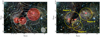 |
Fig. 1. JHK false−color VVV image of 7′×5′ size and centered at αJ2000 = 14 : 45:12.2, δJ2000 = −59:49:27.6. a) White curves are radio continuum flux levels at 843 MHz (SUMSS) revealing the presence of two peaks “A” and “B” of G316.8−0.1 radio source and identified by Vig et al. (2007). The white ellipse at the right-bottom corner indicates the corresponding radio beam size. Red circles represent the locations and mean sizes given by Dutra et al. (2003) for embedded clusters DBS 89−90−91. b) Yellow circles indicate the adopted “Region A”, “Region B”, and “Region C” used along our work to study different stellar populations (see Sects. 3.2.1 and 3.2.2 for details). These regions were used to build the photometric diagrams showed in Fig. 7. Centers for DBS 89−90−91 clusters are presented with white crosses. |
Region properties and their associated objects.
Taking into account recent information from the surveys indicated above, and given that there are relatively few known bipolar H II regions in the Galaxy, our investigation of the radio source zone G316.8−0.1 with new data and taking a global view are needed in order to better understand the different processes involving young stars and their connection with the environment. In particular, Samal et al. (2018) indicate that they were not able to identify the exciting source of G316.8−0.1. Therefore, we performed a deep and detailed photometric and astrometric study of the stellar populations in the zone of the DBS 89−90−91 embedded clusters, and complement our investigation with information on the surrounding ISM. We also reanalyzed the fundamental parameters of these clusters and the ISM.
The structure of the paper is as follows. Observational data are presented in Sect. 2. Different surveys with radio data and photometric and astrometric information are also briefly described. The analysis of our results is presented in Sect. 3. Finally, a discussion and conclusions are presented in Sects. 4 and 5, respectively.
2. Observational data
2.1. Photometric data
We used photometric data for the objects located in the field of view (FOV) presented in Figs. 1 and 2. We used the JHK stacked images of the VVV survey and downloaded them from the VISTA Science Archive (VSA website1). The selected images were obtained on April 3, 2010, with an exposure time of 10 seconds in each band. The region under study has a high level of stellar concentration with a highly variable background in the IR. We performed point spread function (PSF) photometry (Stetson 1987) on the VSA images using the image reduction and analysis facility (IRAF)2 DAOPHOT package to compute instrumental magnitudes. The obtained photometric tables were aperture-corrected for each filter in order to bring them to a final aperture size of 17 pixels in radius. Tables of different filters were combined using DAOMASTER code (Stetson 1992). The calibration was carried out using the 2MASS catalog and the following transformation equations:
 (1)
(1)
 (2)
(2)
 (3)
(3)
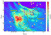 |
Fig. 2. Deconvolved radio continuum image at 843 MHz (SUMSS) of the same size and center as Fig. 1. Selected regions A, B, and C (see Sect. 3.2.1) are indicated by large yellow circles. Red and blue lines show the section, extension, and inclination of the cuts made in different parts of the H II region. Symbols indicate the identified members in each studied region and identified YSOs in the surrounding neighborhood. Green symbols correspond to MS stars and red ones to stars with a probable IR excess. Yellow and orange symbols indicate Class I and II YSOs, respectively. Circles correspond to those identified using K band and WISE data, triangles those using only WISE data, and squares those identified using GLIMPSE data. Large red squares indicate objects listed in Table B.3. Green symbols with blue edges are the astrophotometric members presented in Table C.2. |
where JHK are the 2MASS magnitudes, and (jhk)inst are the instrumental ones. The coefficients (jhk)x (x = 0, 1, 2) were computed using the FITPARAMS task of the IRAF PHOTCAL package. The obtained values are shown in Table 2. We also used the 2MASS catalog to complement the magnitudes of the bright stars (J < 13.5, H < 12, K < 11).
Calibration coefficients used for IR observations together with the corresponding root-mean-square (rms) fit values.
Additionally, we included the optical photometric data (G, GBP, and GRP bands) given by the Gaia early data release 3 (EDR3) covering the field of view (FOV). As the fluxes of the studied objects can significantly change between optical (Gaia) and IR bands, we did not consider photometric error constraints for optical bands, but a wide range of error (e < 0.5) for NIR bands.
We also considered the mid-infrared (MIR) photometric information from the following catalogs: (a) WISE (Cutri 2014) at 3.4, 4.6, 12, and 2 μm bands (W1, W2, W3, and W4, respectively); (b) Spitzer−GLIMPSE (Benjamin et al. 2003) at 3.6, 4.5, 5.8, and 8.0 μm bands; and (c) Midcourse Space Experiment (MSX; Price et al. 2001) at 8.3, 12.1, 14.7, and 21.3 μm bands with a spatial resolution of ∼18″. For WISE and GLIMPSE catalogs, we selected sources with a photometric uncertainty of < 0.2 mag in all bands and a signal-to-noise ratio of > 7 for WISE sources. In the case of the MSX point source catalog (Egan et al. 2003), sources were selected with variability and reliability flags of zero and flux a quality Q > 1 in all bands.
We then employed the STILTS3 tool to manipulate tables and to crossmatch the optical Gaia data, the NIR 2MASS/VVV data, and MIR WISE data in the FOV. In this procedure, we considered a maximum searching distance of 1″ to match objects among 2MASS, VVV, and Gaia catalogs and a distance of 4″ for the WISE catalog. Additionally, to minimize possible mistaken associations between NIR and MIR catalogs, we considered a difference of lower than five magnitudes between the K and W1 bands. We obtained a catalog with photometric information for 3350 point objects in the FOV (see Fig. 1). The photometric errors in the catalog were those provided by the DAOPHOT and DAOMASTER codes and the corresponding source catalogs.
2.2. Radio data
We study some characteristics of the G316.8−0.1 radio source consulting suitable surveys. We employed the Sydney University Molonglo Sky Survey (SUMSS; Bock et al. 1999), which provides data with radio continuum emission at 843 MHz with a synthesized elliptical beam of 45″ cosec |δ| × 45″. We used these to study the density flux intensity and the angular size of the radio source G316.8−0.1 and to confirm the absence of other radio H II regions in the environment close to this H II region (Fig. 2). The Southern Galactic Plane Survey (SGPS; McClure-Griffiths et al. 2005) H I datacube provides data of the Galactic plane over the fourth quadrant with  angular resolution, ΔV = 0.82 km s−1 velocity resolution, and 0.2 K rms noise brightness temperature (Tb). We use this survey to study the kinematic distance to G316.8−0.1 (Fig. 3).
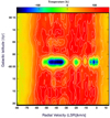 |
Fig. 3. Radio image at 21 cm (SGPS) of the H I emission distribution of the G316.8−0.1 radio source (l ∼ 317°). H I absorption in the line of sight is indicated in blue and green. Contours have a spacing of 28 K, with the first being at −78 K. The color bar shows the colors associated with different H I brightness temperature values in Kelvin. |
2.3. Astrometric data
We performed an astrometric analysis of the region using the Gaia EDR3. The reference epoch for Gaia EDR3 is 2016.0 and the catalog is almost complete between magnitudes G = 12 and G = 17.
The astrometric data include the five astrometric parameters (position, parallax, and proper motion) for 1468 billion sources. The uncertainties in position, parallax, and proper motion according to the G magnitude are given in Table 3 (Lindegren et al. 2021). The parallax zero point deduced from the extragalactic sources is about −17 μas (Lindegren et al. 2021). The probabilistic distances derived from the parallax are obtained from Bailer-Jones et al. (2021).
Typical uncertainty values for the five-parameter solutions at different Gaia magnitudes (G).
We adopted a circular region of 3.0′ in radius with its center at (αJ2000, δJ2000) = (14:45:12.0, −59:49:12.0). We then selected 898 stars from Gaia EDR3 of which 801 have the five astrometric parameters necessary for our analysis. To ensure the quality of the astrometric results, we make a selection of the stars taking into account the following criteria: (i) the renormalised unit weight error (RUWE) parameter ≤1.4 (Lindegren et al. 2021) because this value is a quality indicator of the astrometric solution; (ii) stars with a Dup parameter of equal to 1 are not selected because this value indicates probable astrometric or photometric problems; (iii) the values of the components of the proper motion are between −20 and +20 mas yr−1 because a previous visual inspection of the vector point diagram (VPD) of the region showed low proper motions for the possible embedded clusters; (iv) stars without magnitude G are not included; (v) systematic errors in the proper motion due to the angular scale of the studied region were also analyzed. In our sample, no star had a proper motion within uncertainties of smaller than the systematic error given in Table 7 of Lindegren et al. (2021). With these conditions, the sample is reduced to 754 sources.
3. Analysis and results
3.1. Interstellar medium
Following Vig et al. (2007), the main peaks of the radio source G316.8−0.1, namely A and B, are associated with those of the IRAS source (see Table 1). As SUMSS radio data are of relatively low spatial resolution, we carried out a deconvolution procedure with them in order to obtain a more detailed picture of the zone (Fig. 2). The Richardson-Lucy method (Richardson 1972; Lucy 1974) was applied, because it is able to preserve the flux information. We then obtained some characteristic profiles of the resulting image, choosing those including peaks A and B (see Figs. 2 and 4). The shape of G316.8−0.1−A is approximately circular with a deconvolved angular size of θl = θb = 66″, which was obtained from the measured half-power beam width (HPBW). The cut made to G316.8−0.1−A and shown in Fig. 4b has a double peak (see Sect. 4.3 for details). The shape of G316.8−0.1−B is irregular and somewhat elongated along the Galactic plane. Its deconvolved HPBW values at each axis are θl = 141″ and θb = 38″, whereas the corresponding geometric mean is (θl × θb)1/2 ≃ 73″.
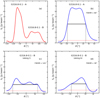 |
Fig. 4. H I profiles obtained with: (a) diagonal cut at l = 316°.79, indicated with a red line in Fig. 2; (b) cut at l = 316°.81, indicated with a blue line in Fig. 2, where the HPBW of the G316.8−0.1−A profile is its deconvolved angular size; (c) cut at l = 316°.77, indicated with a blue line in Fig. 2, where the HPBW of the G316.8−0.1−B profile is the angular size of the part along the Galactic plane; (d) cut at l = 316°.79, indicated with a blue line in Fig. 2, where the HPBW of the G316.8−0.1−B profile is the angular size of the part perpendicular to the Galactic plane. Red slashed lines represent the adopted background levels. |
We estimated the flux density at 843 MHz for both regions. Using the tvstat AIPS 4 task, we obtained the background average flux density, Sbg = 2.6 × 10⁻² Jy beam−1, from the mean flux density values at three different positions near these sources. The root mean square of Sbg was rmsSbg = 5.2 × 10⁻² Jy beam−1 and we used this to distinguish the signal from the noise. The lower isophote presented in Fig. 2 corresponds to 0.5 Jy beam−1, which is more than three times the rmsSbg value. We obtained the density flux value of each source and then subtracted the same Sbg value for both regions. The results were SνRA = 18 Jy and SνRB = 9 Jy for sources G316.8−0.1−A and B, respectively. The density flux value measured across the whole H II region is Sν = 28 Jy.
When an ionized gas cloud is examined over the entire frequency range, the received signal will be affected by opacity depending on the frequency of the energy. At high frequencies, the plasma must become optically thin and the spectrum of the observed radio emission will become approximately flat. This is the behavior observed with the flux density measured at three different frequencies (see Fig. 5).
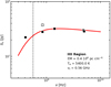 |
Fig. 5. Flux density measured at five different frequencies (see Sect. 3.1) for the whole G316.8−0.1 H II region. Red curve indicates the best-fitted radio spectrum of a thermal free−free emission model the indicated parameters. Only filled squares were used in the fits. Dashed vertical line shows the turnover frequency (νt) value. |
The spectral index α (S ∼ ν−α) can be obtained from the measured flux density at two different frequencies, ν1 and ν2 (α = log(S1/S2)/log(ν2/ν1)). Using ν1 = 843 MHz, Sν1 = 28 Jy and ν2 = 1415 MHz, Sν2 = 32 Jy (Shaver et al. 1981), we obtained α = −0.26. We estimated another value for the spectral index, α = 0.05, using ν1 = 1415 MHz, Sν1 = 32 Jy and ν2 = 4850 MHz, Sν2 = 30 Jy (Kuchar & Clark 1997). The value of Sν = 37.5 Jy for ν = 843 MHz (Vig et al. 2007) was discarded because it is higher than our estimation, which is probably because it was obtained in a larger region (∼30 arcmin2) and does not correspond to the study region of this work. In order to obtain the best adjustment of the entire flux density shown in Fig. 5 and to know the range of values of the spectral index parameter associated with this H II region, we incorporated two additional values, Sν = 22.3 Jy at ν2 = 408 MHz and Sν = 28.7 Jy at ν2 = 5000 MHz, both provided by Shaver & Goss (1970).
We employed the 21 cm line emission map of the SGPS to study the H I absorption in the line of sight, which is indicated in Fig. 3 in blue and green. This absorption could be a consequence of the temperature difference between the H II region and the distribution of the H I gas. The former has a continuum temperature (Tc) higher than the Tb of the H I gas. In this case, components A and B of the radio source G316.8−0.1 could not be angularly resolved; therefore, we were only able to perform a global study, obtaining the same radial velocity measurement for both. In order to determine the approximate radial velocity of this radio source, we obtained the “on” source profile in the brightest region of this using the H I data cube. Later, we obtained the “off” profile. For this, we obtained the intensity profile in three different places in the environment of the H II region; after this we average these three profiles and obtained the “off” profile. Assuming that the “on” and “off” spectra both sample the same gas, subtraction of one from the other removes the common emission. Figure 6 shows the “on” minus “off” profile. The absorption feature observed in this figure at −44 km s−1 Local Standard of Rest (LSR) radial velocity corresponds to a kinematic distance of 3.3 ± 0.6 kpc for sources G316.8−0.1−A and B, according to the galactic rotation model of Brand & Blitz (1993). These results are in agreement with those obtained by Caswell et al. (1995). The value of the radial velocity at −44 km s−1 is a relatively close match to the 13CO (1−0) molecular line (emission, MOPRA telescope) and H I 21 cm data (absorption, SGPS survey) for G316.8−0.1 obtained during the Red MSX survey (Busfield et al. 2006). Longmore et al. (2007) measured the radial velocity, VLSR, of the NH3(1,1) and NH3(2,2) molecular lines at ∼24 GHz with the Australia Telescope Compact Array (ATCA) with a spectral resolution of 0.2 and 12.7 km s−1, respectively, and NH3(4,4) and NH3(5,5) molecular lines, with spectral a resolution of 0.8 km s−1. The results obtained by these authors vary from −37.3 ± 0.3 to −42.2 ± 0.8 km s1.
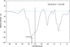 |
Fig. 6. Relative intensity of the G316.8−0.1 (“on-source”) subtracted from the average of three sources of its environment (“off-source”). Higher-intensity absorption would indicate the location of the H II region. The vertical line at −40 km s−1 shows the velocity of the 13CO (1−0) molecular line (emission) detected with the MSX survey by Busfield et al. (2006). The horizontal light blue line shows the zero value from which the absorption intensity is measured. |
To estimate other physical parameters of these regions, we adopted the Gaussian model presented by Mezger & Henderson (1967). We computed the Stromgreen linear radius (Rs) as the deconvolved source angular size and the H II region distance of 2.9 kpc (see Sect. 4.1). Additionally, we obtained the electronic density (Ne), the total mass of ionized hydrogen (MH II), and the emission measure (EM) using equations and numerical values of each factor published by Mezger & Henderson (1967). For both regions, we assumed the same electronic temperature (Te) value of 5400 K obtained by Caswell et al. (1995). The calculated values for all of these parameters are shown in Table 4.
Physical parameters of radio sources G316.8−0.1−A and B.
We estimated the optical depth, τν, using the integral of the absorption coefficient along the line of sight. For the radio domain, Mezger & Henderson (1967) gave the following useful expression, which is valid for frequencies smaller than 10 GHz:
 (4)
(4)
The integral of the square of the electron density along the line of sight is the EM. We computed the frequency at which τ = 1, which is known as the turnover, employing the EM value of 0.4 × 10⁶ pc cm−6 corresponding to the entire G316.8−0.1 radio source. A typical frequency of turnover for free−free emission is 1 GHz and we obtained a value of ν = 0.56 GHz.
3.2. Stellar population methods
As revealed by NIR images (see Fig. 1), embedded clusters DBS 89−90−91 are characterized by a relevant H II background emission. An overdensity of bright stars is evident for DBS 89. However, DBS 90 and DBS 91 are fainter and a high absorption dust lane (SDC G316.786−0.044; Peretto & Fuller 2009) is present between them.
To study the stellar population associated with these embedded clusters, we selected three circular regions identified as Region A, Region B, and Region C. Regions A and B were defined to include most of the cluster probable members. Therefore, their location and sizes were obtained using an iterative procedure looking for star overdensities in the IR image (Fig. 1) and the maximum amount of cluster members after applying our photometric method (see Sect. 3.2.1). Region C was defined as a result of our astrometric analysis. This analysis stipulates that a stellar group must show an overdensity in the sky as well as in the VPD. In Sect. 3.2.2, we show how we first detect the overdensity in the VPD and then identify the overdensity in the sky by visual inspection. Final adopted centers and sizes for each region are presented in Table 1 and plotted on Fig. 1. We note that, whereas Region A includes the G316.8−0.1−A radio source peak, Region B is located to the west of the G316.8−0.1−B peak.
3.2.1. Photometric analysis
Photometric color−color and color−magnitude diagrams (TCDs and CMDs, respectively) of the point objects located in Regions A and B are presented in Fig. 7(a–f). All CMDs in each region clearly reveal the presence of differential reddening. We studied these diagrams and classified the objects following a procedure based on the computation of several reddening-free parameter values (see Baume et al. 2020 for details), the photometric information at Gaia bands, and following the color conditions from WISE bands given by Koenig et al. (2012). Therefore, we could carry out a selection of different kinds of objects: (a) early main sequence (MS) stars, (b) objects with IR color excess, and (c) objects identified as class I and class II YSOs. The remaining objects were not classified and they were considered as field stars.
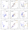 |
Fig. 7. Gaia and IR photometric diagrams for Regions A, B, and C. Symbols have same meaning as in Fig. 2, but in this case hollow blue circles correspond to objects in Table C.1. Light gray circles indicate unclassified stars and most of them are field population stars (See Sect. 3.2.1 for details). Particular objects described in Sect. 4.3 are identified. Green and blue curves are the MS (see text) shifted according to the adopted distance modulus with and without absorption and reddening, respectively. Red lines indicate the considered reddening path. Adopted reddening values for Regions A and C and Region B are those presented in Table 5 for DBS 90−91 and DBS 89, respectively. |
In the above procedure, we used the MS values given by Sung et al. (2013), Koornneef (1983), and the photometric relationships for Gaia filters indicated on the official Gaia web page5. We also considered a normal interstellar reddening law (RV = AV/EB − V = 3.1) and the reddening model given by Wang & Chen (2019). The adopted extreme values for color excesses are presented in Table 5 as E(B − V)min and E(B − V)max. Both border values were used to identify MS stars, while only the lower one was used to select objects with IR color excess (IR objects). Values for the other color indices (EICmin and EICmax) were computed using the Wang & Chen (2019) model. These border values are also indicated in the photometric diagrams by the location of the shifted MS (EICmin) and the point of the reddening vector (EICmax).
Main Parameters of the embedded clusters.
The upper MS has an almost vertical shape over the IR CMDs, which prevents us from estimating precise distance values. After trying several distances (from 2.2 to 3.4 kpc), we obtained the same objects as those suggested by Gaia EDR3 photometric information as probable members for Region B. However, for each distance, we obtained a different set of objects with IR information as probable cluster members. Finally, we considered the distance value of 2.9 kpc obtained with the astrophotometric analysis (see Sect. 4.1). These CMDs also provided an estimation of the foreground color excess E(B − V)min of the studied young stellar populations. The excess values confirmed that Region A objects are much more reddened than those of Region B, as is suggested by Fig. 1.
For these clusters, and following the analysis of Vig et al. (2007), the spectral types of the adopted MS stars and IR objects were estimated by de-reddening their positions in a J versus J − H diagram. As this diagram alleviates the need for K band, possible IR excess problems are minimized. However, this procedure depends on the precision with which the distance is known, providing in our case an approximate result. Therefore, we performed only a rough classification using the four labels O−, O+, B−, and B+, where O and B letters indicate O and B type stars, and minus and plus symbols mean early and late stars inside each type, respectively. The numbers of the different kinds of objects identified for each studied cluster and the corresponding adopted spectral types are presented in Tables 5 and A.1, respectively.
To look for YSO candidates in the surroundings of IRAS 14416−5937, we searched in a region centered at (l, b) = (316°.8, −0°.06) within a circle of 0.1 degrees in radius. We adopted the YSO candidate classification scheme described in Koenig et al. (2012), Gutermuth et al. (2009), and Lumsden et al. (2002), for the WISE, GLIMPSE, and MSX data, respectively.
For the WISE sources, we used the WISE All−Sky Source Catalog (Wright et al. 2010). We selected sources with photometric flux uncertainties of lower than 0.2 mag and a S/N of greater than 7 in the W1, W2, and W3 bands. Following the criteria of Koenig et al. (2012) for these sources, we first discarded the non-YSO sources with excess IR emission, such as polycyclic aromatic hydrocarbons (PAH)-emitting galaxies, broad-line active galactic nuclei (AGNs), unresolved knots of shock emission, and PAH emission features. After that process, from the 248 sources from the list, only 34 were kept, of which we detected 8 WISE Class I sources (i.e., sources where the IR emission arises mainly from a dense envelope, including flat-spectrum objects). We also detected 26 candidate Class II sources (i.e., pre-main sequence stars with optically thick disks). As the last step, we also rejected one Class II source (J 144552.74−59541) whose magnitudes satisfied (W1 − W3 < −1.7 × (W3 − W4 + 4.3)), because according to Koenig et al. (2012) it could be considered to not have sufficiently reddened colors, finally obtaining 25 class II sources.
The GLIMPSE sources were kept if their photometric uncertainties were lower than 0.2 mag in all four IRAC bands (3.6, 4.5, 5.8, and 8.0 μm). Taking these constraints into account, a total of 217 sources were selected. After applying the criteria of Gutermuth et al. (2009), we detected four Class I and ten Class II YSO candidates. All the detected YSO candidates but two were also detected by Vig et al. (2007). It is worth mentioning that these authors carried out searches for YSOs in areas slightly different (∼30% bigger) from the one used in this work. Samal et al. (2018) detected the same four Class I YSO candidates. In addition, we searched in the MSX Point Source Catalog (PSC; Egan et al. 2003) looking for MYSOs and CH II region candidates following the criteria of Lumsden et al. (2002). We selected the sources with variability and reliability flags with values of 0 and flux qualities above 1 in all four MSX bands (8, 12, 14, and 21 μm). Only two sources from 32 fulfill these criteria. One of these is an MYSO (G316.8083−00.0500) and the other is a CH II candidate. Neglecting the constraints of variability and reliability flags, we additionally identified the MSX MYSO candidate G316.8112−00.0566, already cataloged by Busfield et al. (2006). All WISE, GLIMPSE, and MSX YSO candidates are listed in Tables B.1–B.3, respectively.
3.2.2. Astrometric analysis
Astrometric data (position and proper motion) show that a star cluster can be seen as an over-density in the sky as well as in the VPD. The astrometric method of analysis of these overdensities allows us to carry out an independent identification of their members and a determination of their astrometric parameters.
First, we analyzed the VPD overdensity adopting the mathematical model suggested by Vasilevskis et al. (1958) and the technique based on the maximum-likelihood principle developed by Sanders (1971). This model assumes that the proper motion distribution (Φi(μxi, μyi)) of the region selected consists in the overlapping of two bivariate, normal frequency functions.
 (5)
(5)
where ϕ1i is a circular distribution for cluster stars, ϕ2i is an elliptical distribution for field stars, μxi, μyi are the proper motion of the ith star in x and y, respectively. (see Fig. 8).
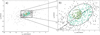 |
Fig. 8. VPD of the 754 stars studied using astrometric Gaia data. Panel (b) presents a zoomed-in view of the central part of panel (a). The ellipse and the slashed circle represent the enclosed curves for the selected objects for the field and cluster populations, respectively (see Sect. 3.2.2). Green dots are the 353 stars selected from the Gaia EDR3 catalog and the yellow hollow symbols represent the 110 possible members obtained in this paper. |
The circular and elliptical distributions take the following form:
![Mathematical equation: $$ \begin{aligned} \phi _{1i}(\mu _{xi},\mu _{{ y}i})= \frac{N_c}{ 2\pi \sigma _{c}^2} \times \exp \left[-\frac{(\mu _{xi}-\mu _{xc})^2 + (\mu _{{ y}i}- \mu _{{ y}c})^2}{2\sigma _{c}^2}\right], \end{aligned} $$](/articles/aa/full_html/2023/06/aa43014-21/aa43014-21-eq7.gif) (6)
(6)
and
![Mathematical equation: $$ \begin{aligned} \phi _{2i}(\mu _{xi},\mu _{{ y}i})= \frac{N_f}{ 2\pi \sigma _{xf}\sigma _{{ y}f}} \times \exp \left[-\frac{(\mu _{xi}-\mu _{xf})^2}{2(\sigma _{xf})^2} - \frac{(\mu _{{ y}i}- \mu _{{ y}f})^2}{2(\sigma _{{ y}f})^2}\right], \end{aligned} $$](/articles/aa/full_html/2023/06/aa43014-21/aa43014-21-eq8.gif) (7)
(7)
where the symbols σxf, σyf are the elliptical dispersion for the field stars, σc the circular dispersion for the cluster stars, μxf, μyf the mean proper motion of the field star, and μxc, μyc the mean proper motion of the cluster. Nc is the number of cluster members, and Nf the number of field stars. These parameters were found by applying the maximum-likelihood principle. Before applying the model, the VPD of the N stars was rotated over angle β to make its axes coincident with the field distribution axes (see Fig. 8.)
We were then able to determine the membership probability for the ith star from
 (8)
(8)
Therefore, the Nc stars with the highest Pi(μxi, μyi) values are considered as members.
This method makes it possible to remove most of the field stars from the sample. The percentage of stars that have been removed depends on the distribution of the stars’ proper motions. To know the degree of effectiveness, we evaluated the membership using the index E, following Shao & Zhao (1996):
![Mathematical equation: $$ \begin{aligned} E= 1- \frac{N \sum _{i=1} ^ {N} P_{i} [1- P_{i}] }{ \sum _{i=1} ^ {N} P_{i} \sum _{i=1} ^ {N} [1-P_{i}] }. \end{aligned} $$](/articles/aa/full_html/2023/06/aa43014-21/aa43014-21-eq10.gif) (9)
(9)
When the moving group and the field stars are perfectly separated, we obtain the maximum value of E = 1; therefore E is an estimate of the contamination of the selected sample. Therefore we applied the analysis to the 754 stars selected from the Gaia EDR3 catalog (see Sect. 2.3), and we obtained the following parameters: μα cos δc, μδc, σc, Nc (see Table 6). From Eq. (8), we calculated the membership probability for each star and identified the 110 probable proper-motion members (see Fig. 8). The resolution of Eq. (9) gave E = 0.73, indicating a good separation between the field stars and those of the moving group.
Astrometric parameters of the stellar groups.
In order to identify embedded clusters, we then applied the other astrometric condition that characterizes them, namely the overdensity in the sky. In Fig. 9, the positions of stars following the Gaussian elliptical distribution are presented with green filled symbols (353 stars) and the 110 possible proper-motion members are presented with yellow hollow symbols. The analysis of this chart allowed us to identify two possible stellar groups of field stars with the same proper motion: one denominated group B with 18 stars (indicated with yellow filled symbols and identified with the embedded cluster DBS 89) and the other denominated group C with 13 stars (represented by blue filled symbols). The astrometric members of each of these groups are presented in Table C.1 and their astrometric parameters in Table 6. The astrometric analysis did not detect any spatial overdensity in Region A.
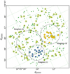 |
Fig. 9. Finding chart of probable astrometric members. Hollow yellow symbols and green dots have the same meaning as in Fig. 8. Full yellow and blue symbols indicate the astrometric members of group B and group C, respectively (see Sect. 3.2.2). Selected regions A, B, and C (see Sect. 3.2.1) are indicated by large dashed line circles. |
3.2.3. DBS89 members
The comparison of the 18 possible astrometric members with the 19 possible photometric ones shows the following results for the DBS89 embedded cluster: (a) There are nine stars in common between the two analyses, which we have denominated astrophotometric members (see Table C.2). (b) The photometric members identified as 2MASS stars J14445838-5948416 and J14450022-5949489 in Table A.1 are not astrometric members. (c) For the remaining possible photometric members presented in Table A.1, no counterpart was found in Gaia EDR3. (d) Finally, the astrometric members identified as “nm” in Table are not photometric members.
3.2.4. Energetic balance
To elucidate whether or not the embedded clusters DBS 89−90−91 could have generated the H II region, we computed the excitation parameter μ = RS
 of G316.8−0.1. This represents the number of Lyman photons that had to be absorbed by the HI to create the H II region (see Table 4).
Additionally, the knowledge of the number of Lyman photons emitted by the brightest stars of DBS 89−90−91 is important in order to evaluate their capacity to generate the H II region. Therefore, we computed the ionization parameter (U) given by Wilson et al. (2013) as
 (10)
(10)
where α2(Te) is the total recombination coefficient of hydrogen, excluding captures to the ground level. The value of the α2(Te) coefficient was computed using the expression of Spitzer (1978) and Te = 5400 K (Caswell et al. 1995). For the ionization parameter (U), the number of Lyman ionization photons provided by earlier stars than B+ (Sternberg et al. 2003) of possible members of DBS 89−90−91 was calculated. We considered atmosphere models for hot stars with solar metallicity and luminosity Class V. We decided to use spectral type (ST) B 1.5 for B− stars, ST = O 8 for O+ stars, and ST = O 5 for O− stars. Embedded cluster DBS 89 (Region B) has 11 B−, 2 O+, and 2 O− stars, and all of them contribute a U value of ∼116 [pc cm−2]. Embedded cluster DBS 90−91 (Region A) has five B− stars and the particular objects (Objs 1, 2, and 3) are described in Sect. 4.3. The spectral type of these Objs is possibly B− (Obj 1), O− (Obj 3), and Wolf-Rayet (WR), (Obj 2). Law et al. (2002) studied the ionizing fluxes of WR stars and the Lyman continuum flux appears independent of the WR spectral type, being 47.44 ≤ Q ≤ 50.51. As Vig et al. (2007) adopted one ST earlier than O6 for Obj 2, we decided to assign this the number of Lyman ionization photons provided by ST O 5. In this way, DBS 90−91 contribute to the ISM with the Lyman ionization photons of six B− and two O− stars, resulting in a U value of ∼109 [pc cm−2]. If we only considered the Lyman ionization photons of WR star as ST = O 5, the U value would be ∼86 [pc cm−2]. After that, we compare parameters μ and U and we find U ≫ μ, which follows the relation  if we take into account the WR star probable member of DBS 90−91, and
  = 2.0 if we consider the DBS 89 embedded cluster.
4. Discussion
4.1. DBS89 cluster distance
The distance of a star-forming region is not easy to estimate, in particular in the fourth Galactic quadrant because of the ambiguity in distance. From research carried out on the G316.8−0.1 H II region, with observations obtained by different authors at different spectral ranges, distance values have been proposed in the range from 2.5 (Caswell & Haynes 1987) to 3.3 kpc (Caswell et al. 1995). To resolve the kinematic distance ambiguity, Busfield et al. (2006) searched some types of 13CO and H I spectral profiles of MYSOs observed with the Mopra 22 millimetre wave telescope combined with SGPS H I data.
We were able to estimate an astrometric distance to the DBS 89 cluster using the Bailer-Jones et al. (2021) distance catalog obtained from Gaia EDR3 parallaxes, selecting the nine astrophotometric adopted members presented in Sect. 3.2.3 Studies by Bailer-Jones et al. (2021) on Gaia EDR3 show that for stars with a fractional error of f = σπ/π ≤ 0.1, the inverse of the parallax gives us a good estimate of the distance. For the cases in which f is greater, it is convenient to use the Bailer-Jones et al. (2021) distance catalog, where the authors use a three-dimensional model of the Galaxy, and include the interstellar extinction and the magnitude limit of Gaia. To infer the distance, they develop two models: the geometric model where they use parallax and its error; and the photogeometric model where, in addition to parallax, they use the color and apparent magnitude of the star. We must take into account that the distances provided by Bailer-Jones et al. (2021) in their catalog incorporated the parallax zero-point correction of −0.017 mas yr−1 derived by Lindegren et al. (2021).
According to Bailer-Jones et al. (2021), those distances corresponding to 0.1 ≤ f ≤ 1 constitute the most important result of their work. However, the analysis shows that using data with a low fractional parallax error allows the uncertainty in distance to be restricted.
Then, to select the best data we limit the f value to f ≤ 0.5. Applying this condition, we do not consider the first two stars in Table C.2 for the distance calculation (EDR3 number 5878925503633099264 and 5878925709791531776).
Finally, to calculate the distance, we must choose between the two methods proposed by Bailer-Jones et al. (2021; geometric and photogeometric). Although we are in a region with high absorption, as all fractional errors are greater than 0.20, we considered that the incorporation of apparent magnitude and color improves our final result. Table C.2 shows the median of the geometric distance posterior (rgeo) and the median of the photogeometric distance posterior (rpgeo). The value obtained for the average distance is rpgeo = 2.9 ± 0.5 kpc. This value is in agreement with that obtained by Busfield et al. (2006), resolving the ambiguity problem.
4.2. Is group C associated with the H II region G316.8−0.1?
Our astrometric analysis (see Sect. 3.2.2) revealed a group of stars with similar proper-motion values and loose spatial concentration. This group covers the indicated Region C, which overlaps the already identified Region A. We calculated the distance to this group of stars, taking into account the same selection criteria applied to determine the distance of the cluster DSB 89. Then, of the 13 possible members, 6 were eliminated by f ≥ 0.5. The remaining 7 members provided an average distance value of rpgeo = 3.1 ± 1.0 kpc. To evaluate the reliability of this group, we built the photometric diagrams of objects located in Region C (see Fig. 7g–i). These diagrams show that all the astrometrically identified stars in Region C suffer from a much lower value of reddening than that adopted for the embedded clusters associated with the H II region G316.8−0.1. Therefore, this group C seems to belong to the foreground field population.
4.3. Particular objects
Some point objects merit particular attention. These are the ones 2MASS identified as J14452143-5949251 (Obj 2), J14452450-5950084 (Obj 3), and J14452625-5949127 (Obj 1). The location of these objects is shown in detail in Fig. 10 and their main features are the following:
-
Obj 1: The spatial location of this object is only 14″ eastward of the main peak of the radio source G316.8–0.1–A and is also almost coincident with the molecular clump C1 identified by Samal et al. (2018). On the other hand, its location over the JHK photometric diagrams is consistent with an early B-type star. Identifying the corresponding WISE and MSX counterparts for this object is not straightforward. We adopted the WISE J144526.30–594914.0 and MSX G316.8112–00.0566 (both at 1.3″; see Table B.3) for this role. We note that in K band images of VVV, an elongated feature also appeared in this place. This feature was considered to be a probable jet by Samal et al. (2018). We classified the adopted WISE counterpart as a class I YSO and its MSX counterpart was considered to be a MYSO by Busfield et al. (2006). Additionally, the main peak of G316.8–0.1–A has an arc shape that resembles a bow shock (see Mac Low et al. 1991). Under this situation, this peak could be a consequence of UV radiation provided by the B-type star and the presence of an accretion disk (Cesaroni et al. 2016). This picture provides support to a monolithic star-formation process given by Krumholz et al. (2009), because they found, using 3D simulations, that the radiation pressure of massive objects could not halt accretion. It should also be noted that most of the masers in the H II region listed by Dalgleish et al. (2018) are located in the surroundings of this object. As maser emission is associated with a coherent velocity field, such as a disk, a jet, or an expanding shell (Moscadelli et al. 2000), this fact reinforces the previous scenario.
-
Obj 2: In this case, this object has a location coincident with the secondary peak of the radio source G316.8–0.1–A and the molecular clump C2 identified by Samal et al. (2018). We classify its WISE counterpart (J144521.58–594925.3) as a class II YSO. This object has been identified as IRS10 by Shaver et al. (1981) and considered to be a probable O 6 type star and the exciting source of the whole H II region. Vig et al. (2007) studied also the spectral classification of this star and assigned it one ST earlier than O 6. More recently, this object was considered by Anderson et al. (2014) to be a WR candidate and a “colliding wind binary” (CWB). This conclusion was based on its location on the JHK photometric diagrams and these authors proposed it be adopted as the counterpart of the ChI∼J144519–59492 source detected in the X-ray ChIcAGO survey.
-
Obj 3: This object has a similar location to Obj 2 on the JHK photometric diagrams and its WISE counterpart (J144524.21–595007.6) was also classified as a class II YSO. It could be another WR star (Mauerhan et al. 2011), but in this location, there is neither a radio peak nor X-ray emission. Therefore, we classify this object as a dubious early O-type star (O−).
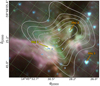 |
Fig. 10. Spitzer color image at the core of the radio source G316.8−0.1−A (ch1 = blue, ch2 = green, ch3 = red), showing the three particular objects described in Sect. 4.3. Light blue symbols indicate masers given by Dalgleish et al. (2018). White curves are radio continuum flux levels at 843 MHz (deconvolved SUMSS) revealing the presence of a double peak. |
4.4. Are DBS 89−90−91 the exciting clusters?
In Sect. 3.2.4, we present the comparison between U and μ parameters. The obtained μ parameter for the radio source G316.8−0.1−A was μ = 71 pc cm−2 and the number of Lyman ionization photons provided in the best case by a WR star (Obj 2), a probable member of DBS 90−91, is U = 86 pc cm−2, which means U > μ. This result shows that the Lymann photons emitted by the WR star are enough to generate the G316.8−0.1−A H II region.
The H II region G316.8−0.1−B has μ = 57 pc cm−2 and the number of Lyman ionization photons provided by earlier star members of DBS 89 is U = 116 pc cm−2, which means U > μ. Both results indicate that G316.8−0.1−A and G316.8−0.1−B are limited by density, and according to the expression ( ), there is an excess of ∼72% of Lyman photons in the former case, and ∼88% in the latter. These photons are not ionizing the gas but are absorbed by the dust, and this latter is heated by them (Kurtz et al. 1994). Based on our investigation of the stellar members employing 2MASS, VVV, and Gaia EDR3 data, we propose that the earliest stars of the clusters DBS 89−90−91 are responsible for the G316.8−0.1 A and B regions.
The presence of YSOs in star-forming regions is indicative of ongoing star-formation activity. Filaments have attracted significant attention as they are believed to be the original source of matter for- and the host zone of star formation. Several studies have demonstrated the role and importance of filaments in the star-formation processes (Schisano et al. 2014; Zhang et al. 2019; Zavagno et al. 2020). In our study, the distribution of the YSOs shown in Fig. 11 is striking. Some of them are seen to be projected onto the dark parental filament identified by Samal et al. (2018), while most of them are seen projected onto the arcs of the 8 μm emission that comes from the PDR. These findings are in agreement with those of other authors (e.g., Bhadari et al. 2022).
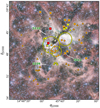 |
Fig. 11. Spitzer color image centered on the G316.8−0.1 radio source (ch1 = violet, ch2 = cian, ch3 = yellow, ch4 = red). Large yellow hollow circles indicate Regions A, B, and C presented in Fig. 1. Symbols are YSOs as presented in Fig. 2. Yellow and orange symbols indicate Class I and II YSOs, respectively. Circles correspond to those identified using K band and WISE data, triangles those using only WISE data, and squares using GLIMPSE data. Big red squares indicate objects listed in Table B.3. Bubbles S109, S110, and S111 presented by Churchwell et al. (2006) are identified. |
5. Conclusions
In this work, we carried out a multiwavelength study of the region of embedded clusters known as DBS 89–90–91. We determined the stellar members of these clusters and their interaction with the ISM. Based on an astrophotometric analysis, we confirm that DBS 89, which is linked to the radio source G316.8–0.1, is located at a distance of 2.9 ± 0.5 kpc from the Sun.
From our photometric analysis of the region, we identified 26 OB-type star member candidates, 10 Class II, and 1 Class I YSO candidate. Among the 26 stars, 9 would be astrophotometric members of DBS 89, 8 would be only photometric members of DBS 89, and the remaining 9 sources would be photometric members of DBS 90–91. We detected several Class I and Class II YSO candidates, two MYSOs, and one CH II distributed throughout the G316.8–0.1 radio source. Some of these objects are seen preferably projected onto the photodissociated region and others are seen projected onto the dark parental filament. The presence of several YSOs located in the regions under study allows us to conclude this is an active star-forming region.
We also estimated the main physical parameters of the H II region and identified the earliest-type stars of the embedded clusters as their main exciting sources. Based on these analyses we were able to improve the current knowledge about the stellar components present in the Sagittarius-Carina arm of our Galaxy and its interaction with the ISM.
IRAF is distributed by NOAO, which is operated by AURA under a cooperative agreement with the NSF.
Acknowledgments
We wish to thank our referee’s suggestions and comments, which improved the original version of this work. This research has received financial support from UNLP “Programa de Incentivos” 11/G158, 11/G168 and 11/G172, and UNLP PPID G005; CONICET PIPs 112-201701-00507CO, 112-201701-00055 and 112-201701-00604, and Agencia I+D+i PICT 2019-0344. The authors want to thank for the use of the NASA Astrophysics Data System, of the SIMBAD database and ALADIN tools (CDS, France). This publication was based on: a) Observations and data products from observations made with ESO Telescopes at La Silla or Paranal Observatories; b) The 2MASS, which is a joint project of the University of Massachusetts and the IPAC/California Institute of Technology, funded by the NASA and the NSF; c) Data products from the WISE, which is a joint project of the University of California, Los Angeles, and the JPL/California Institute of Technology, and is funded by the NASA; d) Observations made with the Spitzer Space Telescope, which is operated by the Jet Propulsion Laboratory, California Institute of Technology under a contract with NASA; e) Data products from the Midcourse Space Experiment. Processing of the data was funded by the Ballistic Missile Defense Organization with additional support from NASA Office of Space Science. This research has also made use of the NASA/ IPAC Infrared Science Archive, which is operated by the Jet Propulsion Laboratory, California Institute of Technology, under contract with the National Aeronautics and Space Administration; f) The SGPS is a project with images obtained at high resolution using the Australia Telescope Compact Array and the Parkes Radio Telescope; g) The SUMSS is a radio imaging survey carried out with the Molonglo Observatory Synthesis Telescope (MOST), Australia and g) This work has made use of data from the European Space Agency (ESA) mission Gaia (https://www.cosmos.esa.int/gaia), processed by the Gaia Data Processing and Analysis Consortium (DPAC, https://www.cosmos.esa.int/web/gaia/dpac/consortium). Funding for the DPAC has been provided by national institutions, in particular the institutions participating in the Gaia Multilateral Agreement.
References
- Anderson, G. E., Gaensler, B. M., Kaplan, D. L., et al. 2014, ApJS, 212, 13 [CrossRef] [Google Scholar]
- Bailer-Jones, C. A. L., Rybizki, J., Fouesneau, M., Demleitner, M., & Andrae, R. 2021, AJ, 161, 147 [Google Scholar]
- Baume, G., Corti, M. A., Borissova, J., Ramirez Alegria, S., & Corvera, A. V. 2020, New A, 79, 101384 [NASA ADS] [CrossRef] [Google Scholar]
- Benjamin, R. A., Churchwell, E., Babler, B. L., et al. 2003, PASP, 115, 953 [Google Scholar]
- Bhadari, N. K., Dewangan, L. K., Ojha, D. K., Pirogov, L. E., & Maity, A. K. 2022, ApJ, 930, 169 [NASA ADS] [CrossRef] [Google Scholar]
- Bock, D. C.-J., Large, M. I., & Sadler, E. M. 1999, AJ, 117, 1578 [Google Scholar]
- Brand, J., & Blitz, L. 1993, A&A, 275, 67 [NASA ADS] [Google Scholar]
- Bronfman, L., Nyman, L.-A., & May, J. 1996, A&AS, 115, 81 [NASA ADS] [Google Scholar]
- Busfield, A. L., Purcell, C. R., Hoare, M. G., et al. 2006, MNRAS, 366, 1096 [NASA ADS] [CrossRef] [Google Scholar]
- Caswell, J. L., & Haynes, R. F. 1987, A&A, 171, 261 [NASA ADS] [Google Scholar]
- Caswell, J. L., Vaile, R. A., Ellingsen, S. P., Whiteoak, J. B., & Norris, R. P. 1995, MNRAS, 272, 96 [NASA ADS] [CrossRef] [Google Scholar]
- Cesaroni, R., Sánchez-Monge, Á., Beltrán, M. T., et al. 2016, A&A, 588, L5 [NASA ADS] [CrossRef] [EDP Sciences] [Google Scholar]
- Churchwell, E., Povich, M. S., Allen, D., et al. 2006, ApJ, 649, 759 [CrossRef] [Google Scholar]
- Corti, M. A., Baume, G. L., Panei, J. A., et al. 2016, A&A, 588, A63 [NASA ADS] [CrossRef] [EDP Sciences] [Google Scholar]
- Cutri, R. M. 2014, VizieR Online Data Catalog, II/328 [Google Scholar]
- Dalgleish, H. S., Longmore, S. N., Peters, T., et al. 2018, MNRAS, 478, 3530 [NASA ADS] [CrossRef] [Google Scholar]
- Dutra, C. M., Bica, E., Soares, J., & Barbuy, B. 2003, A&A, 400, 533 [NASA ADS] [CrossRef] [EDP Sciences] [Google Scholar]
- Egan, M. P., Price, S. D., & Kraemer, K. E. 2003, American Astronomical Society Meeting Abstracts, 203, 57.08 [NASA ADS] [Google Scholar]
- Gaia Collaboration (Brown, A. G. A., et al.) 2021, A&A, 650, C3 [EDP Sciences] [Google Scholar]
- Gutermuth, R. A., Megeath, S. T., Myers, P. C., et al. 2009, ApJS, 184, 18 [Google Scholar]
- Koenig, X., Leisawitz, D., Benford, D., et al. 2012, in American Astronomical Society Meeting Abstracts #219, 320.07 [Google Scholar]
- Koornneef, J. 1983, A&A, 128, 84 [NASA ADS] [Google Scholar]
- Krumholz, M. R., Klein, R. I., McKee, C. F., Offner, S. S. R., & Cunningham, A. J. 2009, Science, 323, 754 [Google Scholar]
- Kuchar, T. A., & Clark, F. O. 1997, ApJ, 488, 224 [NASA ADS] [CrossRef] [Google Scholar]
- Kurtz, S., Churchwell, E., & Wood, D. O. S. 1994, ApJS, 91, 659 [Google Scholar]
- Law, D. R., DeGioia-Eastwood, K., & Moore, K. L. 2002, ApJ, 565, 1239 [NASA ADS] [CrossRef] [Google Scholar]
- Lindegren, L., Bastian, U., Biermann, M., et al. 2021, A&A, 649, A4 [EDP Sciences] [Google Scholar]
- Longmore, S. N., Burton, M. G., Barnes, P. J., et al. 2007, MNRAS, 379, 535 [NASA ADS] [CrossRef] [Google Scholar]
- Lucy, L. B. 1974, AJ, 79, 745 [Google Scholar]
- Lumsden, S. L., Hoare, M. G., Oudmaijer, R. D., & Richards, D. 2002, MNRAS, 336, 621 [NASA ADS] [CrossRef] [Google Scholar]
- Mac Low, M.-M., van Buren, D., Wood, D. O. S., & Churchwell, E. 1991, ApJ, 369, 395 [NASA ADS] [CrossRef] [Google Scholar]
- Mauerhan, J. C., Van Dyk, S. D., & Morris, P. W. 2011, AJ, 142, 40 [NASA ADS] [CrossRef] [Google Scholar]
- McClure-Griffiths, N. M., Dickey, J. M., Gaensler, B. M., et al. 2005, ApJS, 158, 178 [NASA ADS] [CrossRef] [Google Scholar]
- Mezger, P. G., & Henderson, A. P. 1967, ApJ, 147, 471 [Google Scholar]
- Minniti, D., Lucas, P. W., Emerson, J. P., et al. 2010, New A, 15, 433 [Google Scholar]
- Moscadelli, L., Cesaroni, R., & Rioja, M. J. 2000, A&A, 360, 663 [NASA ADS] [Google Scholar]
- Peretto, N., & Fuller, G. A. 2009, A&A, 505, 405 [NASA ADS] [CrossRef] [EDP Sciences] [Google Scholar]
- Price, S. D., Egan, M. P., Carey, S. J., Mizuno, D. R., & Kuchar, T. A. 2001, AJ, 121, 2819 [NASA ADS] [CrossRef] [Google Scholar]
- Richardson, W. H. 1972, J. Opt. Soc. Am. (1917–1983), 62, 55 [Google Scholar]
- Saito, R. K., Hempel, M., Minniti, D., Lucas, P. W., et al. 2012, A&A, 537, A107 [NASA ADS] [CrossRef] [EDP Sciences] [Google Scholar]
- Samal, M. R., Deharveng, L., Zavagno, A., et al. 2018, A&A, 617, A67 [NASA ADS] [CrossRef] [EDP Sciences] [Google Scholar]
- Sanders, W. L. 1971, A&A, 14, 226 [NASA ADS] [Google Scholar]
- Schisano, E., Rygl, K. L. J., Molinari, S., et al. 2014, ApJ, 791, 27 [Google Scholar]
- Shao, Z., & Zhao, J. 1996, Acta Astron. Sin., 37, 377 [Google Scholar]
- Shaver, P. A., & Goss, W. M. 1970, Aust. J. Phys. Astrophys. Suppl., 14, 133 [NASA ADS] [Google Scholar]
- Shaver, P. A., Retallack, D. S., Wamsteker, W., & Danks, A. C. 1981, A&A, 102, 225 [NASA ADS] [Google Scholar]
- Skrutskie, M. F., & Cutri, R. M. 2006, AJ, 131, 1163 [NASA ADS] [CrossRef] [Google Scholar]
- Spitzer, L. 1978, Physical Processes in the Interstellar Medium (New York: Wiley) [Google Scholar]
- Sternberg, A., Hoffmann, T. L., & Pauldrach, A. W. A. 2003, ApJ, 599, 1333 [NASA ADS] [CrossRef] [Google Scholar]
- Stetson, P. B. 1987, PASP, 99, 191 [Google Scholar]
- Stetson, P. B. 1992, JRASC, 86, 71 [NASA ADS] [Google Scholar]
- Sung, H., Lim, B., Bessell, M. S., et al. 2013, J. Korean Astron. Soc., 46, 103 [NASA ADS] [CrossRef] [Google Scholar]
- Vasilevskis, S., Klemola, A., & Preston, G. 1958, AJ, 63, 387 [NASA ADS] [CrossRef] [Google Scholar]
- Vig, S., Ghosh, S. K., Ojha, D. K., & Verma, R. P. 2007, A&A, 463, 175 [NASA ADS] [CrossRef] [EDP Sciences] [Google Scholar]
- Wang, S., & Chen, X. 2019, The Gaia Universe, 59 [Google Scholar]
- Watkins, E. J., Peretto, N., Marsh, K., & Fuller, G. A. 2019, A&A, 628, A21 [NASA ADS] [CrossRef] [EDP Sciences] [Google Scholar]
- Wilson, T. L., Rohlfs, K., & Hüttemeister, S. 2013, Tools of Radio Astronomy (Berlin: Springer, Berlin Heidelberg) [Google Scholar]
- Wright, E. L., Eisenhardt, P. R. M., Mainzer, A. K., et al. 2010, AJ, 140, 1868 [Google Scholar]
- Zavagno, A., André, P., Schuller, F., et al. 2020, A&A, 638, A7 [NASA ADS] [CrossRef] [EDP Sciences] [Google Scholar]
- Zhang, M., Kainulainen, J., Mattern, M., Fang, M., & Henning, T. 2019, A&A, 622, A52 [NASA ADS] [CrossRef] [EDP Sciences] [Google Scholar]
Appendix A: Photometric members
Probable members of embedded clusters DBS 89 (Region B) and DBS 90−91 (Region A+C) from photometric observations. Equatorial coordinates, JHK magnitudes, approximate spectral classification, and adopted object types are presented.
Appendix B: Young stellar objects
YSO candidates identified from the WISE catalog.
YSO candidates identified from the GLIMPSE catalog.
YSO candidates and one CH II region identified from the MSX catalog sources.
Appendix C: Individual stellar proper motions
Adopted astrometric members for group B and group C.
Gaia EDR3 astrometric parameters of DBS 89 astrophotometric members.
All Tables
Calibration coefficients used for IR observations together with the corresponding root-mean-square (rms) fit values.
Typical uncertainty values for the five-parameter solutions at different Gaia magnitudes (G).
Probable members of embedded clusters DBS 89 (Region B) and DBS 90−91 (Region A+C) from photometric observations. Equatorial coordinates, JHK magnitudes, approximate spectral classification, and adopted object types are presented.
All Figures
|
Fig. 1. JHK false−color VVV image of 7′×5′ size and centered at αJ2000 = 14 : 45:12.2, δJ2000 = −59:49:27.6. a) White curves are radio continuum flux levels at 843 MHz (SUMSS) revealing the presence of two peaks “A” and “B” of G316.8−0.1 radio source and identified by Vig et al. (2007). The white ellipse at the right-bottom corner indicates the corresponding radio beam size. Red circles represent the locations and mean sizes given by Dutra et al. (2003) for embedded clusters DBS 89−90−91. b) Yellow circles indicate the adopted “Region A”, “Region B”, and “Region C” used along our work to study different stellar populations (see Sects. 3.2.1 and 3.2.2 for details). These regions were used to build the photometric diagrams showed in Fig. 7. Centers for DBS 89−90−91 clusters are presented with white crosses. |
| In the text | |
|
Fig. 2. Deconvolved radio continuum image at 843 MHz (SUMSS) of the same size and center as Fig. 1. Selected regions A, B, and C (see Sect. 3.2.1) are indicated by large yellow circles. Red and blue lines show the section, extension, and inclination of the cuts made in different parts of the H II region. Symbols indicate the identified members in each studied region and identified YSOs in the surrounding neighborhood. Green symbols correspond to MS stars and red ones to stars with a probable IR excess. Yellow and orange symbols indicate Class I and II YSOs, respectively. Circles correspond to those identified using K band and WISE data, triangles those using only WISE data, and squares those identified using GLIMPSE data. Large red squares indicate objects listed in Table B.3. Green symbols with blue edges are the astrophotometric members presented in Table C.2. |
| In the text | |
|
Fig. 3. Radio image at 21 cm (SGPS) of the H I emission distribution of the G316.8−0.1 radio source (l ∼ 317°). H I absorption in the line of sight is indicated in blue and green. Contours have a spacing of 28 K, with the first being at −78 K. The color bar shows the colors associated with different H I brightness temperature values in Kelvin. |
| In the text | |
|
Fig. 4. H I profiles obtained with: (a) diagonal cut at l = 316°.79, indicated with a red line in Fig. 2; (b) cut at l = 316°.81, indicated with a blue line in Fig. 2, where the HPBW of the G316.8−0.1−A profile is its deconvolved angular size; (c) cut at l = 316°.77, indicated with a blue line in Fig. 2, where the HPBW of the G316.8−0.1−B profile is the angular size of the part along the Galactic plane; (d) cut at l = 316°.79, indicated with a blue line in Fig. 2, where the HPBW of the G316.8−0.1−B profile is the angular size of the part perpendicular to the Galactic plane. Red slashed lines represent the adopted background levels. |
| In the text | |
|
Fig. 5. Flux density measured at five different frequencies (see Sect. 3.1) for the whole G316.8−0.1 H II region. Red curve indicates the best-fitted radio spectrum of a thermal free−free emission model the indicated parameters. Only filled squares were used in the fits. Dashed vertical line shows the turnover frequency (νt) value. |
| In the text | |
|
Fig. 6. Relative intensity of the G316.8−0.1 (“on-source”) subtracted from the average of three sources of its environment (“off-source”). Higher-intensity absorption would indicate the location of the H II region. The vertical line at −40 km s−1 shows the velocity of the 13CO (1−0) molecular line (emission) detected with the MSX survey by Busfield et al. (2006). The horizontal light blue line shows the zero value from which the absorption intensity is measured. |
| In the text | |
|
Fig. 7. Gaia and IR photometric diagrams for Regions A, B, and C. Symbols have same meaning as in Fig. 2, but in this case hollow blue circles correspond to objects in Table C.1. Light gray circles indicate unclassified stars and most of them are field population stars (See Sect. 3.2.1 for details). Particular objects described in Sect. 4.3 are identified. Green and blue curves are the MS (see text) shifted according to the adopted distance modulus with and without absorption and reddening, respectively. Red lines indicate the considered reddening path. Adopted reddening values for Regions A and C and Region B are those presented in Table 5 for DBS 90−91 and DBS 89, respectively. |
| In the text | |
|
Fig. 8. VPD of the 754 stars studied using astrometric Gaia data. Panel (b) presents a zoomed-in view of the central part of panel (a). The ellipse and the slashed circle represent the enclosed curves for the selected objects for the field and cluster populations, respectively (see Sect. 3.2.2). Green dots are the 353 stars selected from the Gaia EDR3 catalog and the yellow hollow symbols represent the 110 possible members obtained in this paper. |
| In the text | |
|
Fig. 9. Finding chart of probable astrometric members. Hollow yellow symbols and green dots have the same meaning as in Fig. 8. Full yellow and blue symbols indicate the astrometric members of group B and group C, respectively (see Sect. 3.2.2). Selected regions A, B, and C (see Sect. 3.2.1) are indicated by large dashed line circles. |
| In the text | |
|
Fig. 10. Spitzer color image at the core of the radio source G316.8−0.1−A (ch1 = blue, ch2 = green, ch3 = red), showing the three particular objects described in Sect. 4.3. Light blue symbols indicate masers given by Dalgleish et al. (2018). White curves are radio continuum flux levels at 843 MHz (deconvolved SUMSS) revealing the presence of a double peak. |
| In the text | |
|
Fig. 11. Spitzer color image centered on the G316.8−0.1 radio source (ch1 = violet, ch2 = cian, ch3 = yellow, ch4 = red). Large yellow hollow circles indicate Regions A, B, and C presented in Fig. 1. Symbols are YSOs as presented in Fig. 2. Yellow and orange symbols indicate Class I and II YSOs, respectively. Circles correspond to those identified using K band and WISE data, triangles those using only WISE data, and squares using GLIMPSE data. Big red squares indicate objects listed in Table B.3. Bubbles S109, S110, and S111 presented by Churchwell et al. (2006) are identified. |
| In the text | |
Current usage metrics show cumulative count of Article Views (full-text article views including HTML views, PDF and ePub downloads, according to the available data) and Abstracts Views on Vision4Press platform.
Data correspond to usage on the plateform after 2015. The current usage metrics is available 48-96 hours after online publication and is updated daily on week days.
Initial download of the metrics may take a while.