| Issue |
A&A
Volume 671, March 2023
|
|
|---|---|---|
| Article Number | A42 | |
| Number of page(s) | 20 | |
| Section | Cosmology (including clusters of galaxies) | |
| DOI | https://doi.org/10.1051/0004-6361/202244799 | |
| Published online | 03 March 2023 | |
A cross-correlation analysis of CMB lensing and radio galaxy maps
1
Dipartimento di Fisica, Università di Roma Tor Vergata, via della Ricerca Scientifica, 1, 00133 Roma, Italy
e-mail: giulia.piccirilli@roma2.infn.it
2
INFN – Sezione di Roma 2, Universitá di Roma Tor Vergata, via della Ricerca Scientifica, 1, 00133 Roma, Italy
3
Department of Physics, University of Genova, Via Dodecaneso 33, 16146 Genova, Italy
4
INFN – Sezione di Roma Tre, via della Vasca Navale 84, 00146 Roma, Italy
5
Centre for Astrophysics & Supercomputing, Swinburne University of Technology, Hawthorn, VIC 3122, Australia
Received:
23
August
2022
Accepted:
21
November
2022
Aims. The goal of this work is to clarify the origin of the seemingly anomalously large clustering signal detected at large angular separation in the wide TGSS radio survey and, in so doing, to investigate the nature and the clustering properties of the sources that populate the radio sky in the [0.15, 1.4] GHz frequency range.
Methods. To achieve this goal, we cross-correlated the angular position of the radio sources in the TGSS and NVSS samples with the cosmic microwave background (CMB) lensing maps from the Planck satellite. A cross-correlation between two different tracers of the underlying mass density field has the advantage of being quite insensitive to possible systematic errors that may affect the two observables, provided that they are not correlated, which seems unlikely in our case. The cross-correlation analysis was performed in harmonic space and limited to relatively modest multipoles. These choices, together with that of binning the measured spectra, minimize the correlation among the errors in the measured spectra and allowed us to adopt the Gaussian hypothesis to perform the statistical analysis. Finally, we decided to consider the auto-angular power spectrum on top of the cross-spectrum since a joint analysis has the potential to improve the constraints on the radio source properties by lifting the degeneracy between the redshift distribution, N(z), and the bias evolution, b(z).
Results. The angular cross-correlation analysis does not present the power excess at large scales for TGSS and provides a TGSS–CMB lensing cross-spectrum that is in agreement with the one measured using the NVSS catalog. This result strongly suggests that the excess found in TGSS clustering analyses can be due to uncorrected systematic effects in the data. However, we considered several cross-spectra models that rely on physically motivated combinations of N(z) and b(z) prescriptions for the radio sources and find that they all underestimate the amplitude of the measured cross-spectra on the largest angular scales considered in our analysis, ∼10°. This result is robust to the various potential sources of systematic errors, both of observational and theoretical nature, that may affect our analysis, including the uncertainties in the N(z) model. Having assessed the robustness of the results to the choice of N(z), we repeated the analysis using simpler bias models specified by a single free parameter, bg, namely, the value of the effective bias of the radio sources at redshift zero. This improves the goodness of the fit, although not even the best model, which assumes a non-evolving bias, quite matches the amplitude of the cross-spectrum at small multipoles. Moreover, the best fitting bias parameter, bg = 2.53 ± 0.11, appears to be somewhat large considering that it represents the effective bias of a sample that is locally dominated by mildly clustered star-forming galaxies and Fanaroff-Riley class I sources. Interestingly, it is the addition of the angular auto-spectrum that favors the constant bias model over the evolving one.
Conclusions. The nature of the large cross-correlation signal between the radio sources and the CMB lensing maps found in our analysis at large angular scales is not clear. It probably indicates some limitation in the modeling of the radio sources, namely the relative abundance of the various populations, their clustering properties, and how these evolve with redshift. What our analysis does show is the importance of combining the auto-spectrum with the cross-spectrum, preferably obtained with unbiased tracers of the large-scale structure, such as CMB lensing, for answering these questions.
Key words: radio continuum: galaxies / cosmic background radiation / methods: data analysis / large-scale structure of Universe / gravitational lensing: weak
© The Authors 2023
 Open Access article, published by EDP Sciences, under the terms of the Creative Commons Attribution License (https://creativecommons.org/licenses/by/4.0), which permits unrestricted use, distribution, and reproduction in any medium, provided the original work is properly cited.
This article is published in open access under the Subscribe to Open model. Subscribe to A&A to support open access publication.
1. Introduction
The study of the cosmic large-scale structure (LSS) has the potential to shed light on the nature of “dark” physics, which drives the accelerated expansion of the Universe, and to detect deviations from the General Relativity framework. Among the many available LSS probes, extragalactic radio sources possess two important properties: they are bright, and they are less affected by Galactic dust extinction than optical sources. As a result, radio sources can trace the spatial distribution of matter over a large volume of the Universe.
For this reason, radio sources have been extensively exploited to study the LSS of the Universe. Clustering analyses have been performed using wide surveys, such as Faint Images of the Radio Sky at Twenty centimeters (FIRST; Cress et al. 1996), Parkes MIT-NRAO survey (PMN; Loan et al. 1997), 4.85-GHz Green Bank Survey (87GB; Kerr et al. 2019), Westerbork Northern Sky Survey (WENSS; Rengelink 1999), Sydney University Molonglo Sky Survey (SUMSS; Blake et al. 2004b), NRAO VLA Sky Survey (NVSS; Blake & Wall 2002; Overzier et al. 2003; Negrello et al. 2006; Chen & Schwarz 2016), Alternative Data Release of the GMRT Sky Survey (TGSS ADR1; Rana & Bagla 2019), and LOFAR Two-metre Sky Survey (LoTSS, Siewert et al. 2020). These analyses used the angular two-point correlation function to characterize their clustering properties. Similar studies have been performed in harmonics space to estimate the angular power spectrum of the sources in the NVSS (Blake et al. 2004b; Nusser & Tiwari 2015), TGSS ADR1 (Dolfi et al. 2019; Tiwari et al. 2019), and LoTSS (Tiwari et al. 2022) catalogs.
Clustering analyses of radio objects have produced a number of intriguing results. The most remarkable is the amplitude of their angular dipole, which turned out to be significantly larger than ΛCDM expectations (Singal 2011; Gibelyou & Huterer 2012; Rubart & Schwarz 2013; Fernández-Cobos et al. 2014; Tiwari & Jain 2015; Tiwari & Nusser 2016; Colin et al. 2017; Bengaly et al. 2018; Siewert et al. 2021). Anomalously large clustering power has also been detected at low multipoles in the TGSS ADR1 survey (Dolfi et al. 2019; Tiwari et al. 2019) but not in the NVSS catalog (Tiwari & Aluri 2019; Dolfi et al. 2019). A further anomaly is the amplitude of anisotropy measured in the radio synchrotron background at 140 MHz, which is also larger than expected (Offringa et al. 2022). These results can be interpreted as either a challenge to the standard cosmological model or the manifestation of observational systematics that have not been properly accounted for. One example of this second case is given by systematic uncertainties in the flux calibration that can potentially generate a spurious clustering signal on large angular scales. Systematic errors of this type have been identified in both the TGSS ADR1 (Tiwari et al. 2019) and LoTSS-DR1 data sets (Tiwari et al. 2022) and may help in relieving the tension with the ΛCDM model.
Performing a uniform flux calibration is notoriously challenging for all types of wide surveys. Those in the radio bands present two additional problems. The first is represented by the composite nature of radio sources that include local, relatively faint, star-forming galaxies (SFGs) as well as bright and distant radio quasars. They map the underlying mass distribution differently; in other words, they are characterized by different biasing relations and, therefore, possess different clustering properties. Moreover, their relative abundance depends on the redshift and on the radio frequency. Therefore, both the effective biasing and the redshift distribution of the radio sources depend on the survey characteristics and need to be modeled accordingly. The second problem is the small fraction of radio objects with measured spectroscopic redshifts, which makes it impossible to map their spatial distribution and limits clustering analyses to angular two-point statistics. The two-point auto-correlation signal (or, equivalently, the auto-angular power spectrum) of the radio sources depends on the combined effect of the biasing relation and the redshift distribution, so these two functions cannot be estimated independently. One way to alleviate, at least in part, these problems is to cross-correlate the angular distribution of the radio sources with that of a different type of mass tracer. Since observational systematics (such as the aforementioned flux calibration issues) and foreground emissions are not expected to correlate with the LSS, spurious angular clustering signals that may contribute to the auto-correlation signal will not affect the cross-correlation one. Moreover, if the second catalog contains objects with a known bias and redshift distribution, or, better still, if it is an unbiased tracer of the mass field, then it will be possible to infer both the bias model and the redshift distribution of the radio sources.
The gravitational lensing signal of the background objects does trace the underlying mass in an unbiased way, and therefore its maps are ideal for cross-correlating catalogs of radio sources. However, lensing maps, obtained from the images of carefully selected background galaxies (see, e.g., Asgari et al. 2021; Amon et al. 2022), do not cover the same wide areas as the radio surveys. For this reason, we consider here instead the all-sky gravitational lensing maps of the cosmic microwave background (CMB) photons. Cross-correlation analyses of CMB lensing and NVSS radio sources have already been successfully performed, leading to a high significance detection of the cross-correlation signal (Smith et al. 2007; Hirata et al. 2008; Feng et al. 2012; Planck Collaboration XVII 2014; Giannantonio & Percival 2014). Our scope is to expand these studies to other catalogs of radio sources with the aim of inferring their nature, distribution, and clustering properties.
More in detail, our goal is twofold. First, we cross-correlate the angular positions of the TGSS ADR1 radio sources with the Planck lensing maps (Planck Collaboration VIII 2020) to clarify the nature of the large-scale clustering excess seen in the auto-correlation analysis. The detection of a similar excess in the cross-correlation would point to a possible cosmological origin. Secondly, we compare the measured cross-correlation between NVSS, TGSS ADR1, and the CMB lensing maps with theoretical predictions to constrain the biasing function and the redshift distribution of the radio sources, also including the auto-correlation statistics in the analysis. The analysis we perform in this work shares the same goals as the one recently performed by Alonso et al. (2021), the difference being that Alonso et al. (2021) used a newer data set (the LoTSS radio survey) distributed over a much smaller area than the one we consider here. A similar analysis was also performed using the cross-spectrum between the CMB lensing from Atacama Cosmology Telescope (ACT) and the FIRST catalog, leading to constraints on the bias and the typical halo mass of radio-loud active galactic nuclei (AGNs; Allison et al. 2015).
The layout of the paper is as follows. In Sect. 2 we present the data sets (CMB-lensing maps and radio catalogs) used in this work. In Sect. 3 we discuss the theoretical model for the auto- and the cross-angular spectra that we measured from the data using the estimators presented in Sect. 4. The results of the measured spectra, their comparison with theoretical predictions, and the inferred quantities are presented in Sect. 5. In Sect. 6 we estimate the galaxy bias parameter while keeping the redshift distribution model fixed, and in Sect. 7 we explore different tests for assessing the robustness of cross-correlation analysis against possible systematics in the radio catalogs, in the lensing map, or both. Finally, in Sect. 8 we discuss our results and present our main conclusions. Throughout this paper we assume a flat Λ CDM cosmological model characterized by the cosmological parameters of Planck Collaboration VI (2020).
2. Data sets
In this section we briefly describe the data sets considered for our analysis. The CMB lensing maps and the catalogs of radio sources are respectively presented in Sects. 2.1 and 2.2.
2.1. CMB lensing convergence map: Planck data
The Planck satellite has observed the sky in several microwave bands with an unprecedented sensitivity and angular resolution. One of its main scientific achievements is the high precision measurement of the gravitational lensing effect, with the reconstruction of the lensing potential map over 67% of the sky and the measurement of its angular power spectrum in the multipole range 8 ≤ ℓ ≤ 2000 (Planck Collaboration VIII 2020). In this paper, we use one of the maps produced by the Planck collaboration, namely the CMB convergence one. This map was obtained with a minimum variance (MV) estimator that combines the reconstructions from CMB temperature and polarization anisotropies, thanks to which the lensing signal has been detected with a 40σ significance. We use the spherical harmonic coefficients for the lensing convergence provided by the Planck collaboration1 to generate a HEALPix2 (Gorski et al. 2005) map with a resolution parameter Nside = 512. This choice corresponds to an angular resolution of ∼7 arcmin and it is motivated by the fact that we expect negligible contributions to the cross-correlation from scales smaller than these. The Planck collaboration also provides the noise spectrum of the convergence map,  , together with a binary map to mask out the sky area to be excluded from the lensing analysis because of possible residual contamination by Galactic and extragalactic foregrounds (see Fig. 1).
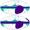 |
Fig. 1. Mollweide projection in Galactic coordinates of the masked areas in the radio samples (purple) and in the Planck CMB lensing convergence map (turquoise). Top panel: NVSS case. Bottom panel: TGSS case. |
2.2. Radio catalogs
The second data set that we considered here consists of two catalogs of extragalactic radio sources derived from the NVSS at 1.4 GHz (Condon et al. 1998) and from TGSS ADR1 (Intema et al. 2017) at 150 MHz.
The NVSS catalog was obtained using the Very Large Array (VLA) telescope3 between 1993 and 1996; while TGSS data have been collected at the Giant Metrewave Radio Telescope4 radio telescope between 2010 and 2012. The two data sets of radio sources are distributed over wide and largely overlapping areas, ΔΩ, covering a fraction of the sky, fsky ≡ ΔΩ/4π, excluding regions in the Southern Hemisphere (with declination δ < −40° and δ < −45° for NVSS and TGSS, respectively) and with low Galactic latitudes (|b|< 5° and |b|< 10° again for NVSS and TGSS). Moreover, following Intema et al. (2017), we removed TGSS objects in the area 25° < δ < 39°, 97.5° < α < 142.5° that were observed in bad ionospheric conditions. Finally, in both samples, the regions around the brightest objects have also been masked out (Nusser & Tiwari 2015). In Fig. 1, we show the portion of masked sky in both TGSS and NVSS catalogs (purple regions) together with the masked area of CMB convergence map (turquoise areas). The sky area is the same as the one considered in the Dolfi et al. (2019) analysis. It excludes regions in which the RMS noise is higher than 5 mJy beam−1 (Intema et al. 2017).
After excluding radio objects in these regions, we end up with 109 940 TGSS sources with fluxes in the interval S150 = [200, 1000] mJy and with 518 894 NVSS sources in the flux range S1.4 = [10, 1000] mJy. The lower limit for the NVSS flux is related to the fact that spurious fluctuations of the surface density of the radio sources have been detected for objects fainter than this value (Blake et al. 2004a). TGSS sources are generally brighter than the NVSS ones and a large fraction of them have a counterpart in the NVSS catalog. The main characteristics of the two catalogs are summarized in Table 1.
Main characteristics of the TGSS and NVSS reference samples.
We used the angular position of these radio sources to build HEALPix maps of objects counts with a resolution parameter Nside = 512 matching the one of the CMB lensing convergence map. We define fluctuations in the objects number counts as
where  is the direction to the pixel,
  is the number of radio objects in the pixel and
  is their mean number per pixel.
3. Angular power spectra models
Cosmic Microwave Background photons propagating from the last scattering surface are deflected by the gravitational potential of the LSS of the Universe. This phenomenon is known as weak gravitational lensing. It re-maps the CMB anisotropies leaving distinctive signatures in their distribution (Lewis & Challinor 2006; Hanson et al. 2010), which can be used to reconstruct the lensing potential:
where Ψ is the underlying gravitational potential, η0 is the conformal time measured today and χ is the comoving distance. We note that this expression is valid for a flat Universe. All the quantities with the asterisk superscript are computed at the last scattering surface redshift, z* ≃ 1100.
Starting from the lensing potential, we use the 2D Poisson equation to define the dimensionless lensing convergence:  . Since the gravitational potential depends on the matter overdensity δm, we can express the CMB lensing convergence as (e.g., Bianchini et al. 2016)
In the above equation, Wκ(z) is the convergence window function and its explicit dependence on the redshift is
where Ωm, 0 is the matter density in units of the critical density at present time, H(z) is the Hubble parameter at redshift z and H0 its value at the present epoch. Once a cosmological model is provided, together with H(z) and χ(z) relations, then the converge in Eq. (3) is determined.
On the other hand, radio surveys provide us with the spatial distribution of detected sources but not with that of the underlying matter. Therefore, to link their density contrast in the sky to that of the matter, one has to specify their redshift distribution, N(z), which accounts for the survey selection function, and also the bias relation between their spatial distribution and the underlying mass density field. In this work we assume a linear, scale free, deterministic bias that can be expressed as a function of redshift only: b(z). The projected density contrast of the radio sources can then be written as
The angular auto-power spectrum of the radio sources is obtained by first expanding  in spherical harmonics,
and then by taking the ensemble average of the expansion coefficients,  , so that
![$$ \begin{aligned} C^{gg}_{\ell }=\frac{2}{\pi } \int _0^{\infty } \mathrm{d}z [W^{g}(z)]^2 \int _0^{\infty }\mathrm{d}k k^2 P(k,z)j^2_{\ell }[k\chi (z)], \end{aligned} $$](/articles/aa/full_html/2023/03/aa44799-22/aa44799-22-eq16.gif)
where P(k, z) is the 3D power spectrum of the mass density fluctuations at redshift z, jℓ are the Bessel functions, and Wg(z) is the window function of the radio sources, which, in our case, is
The CMB lensing convergence–galaxy cross-angular power spectrum is similarly defined as
![$$ \begin{aligned}&C^{\kappa g}_{\ell } = \frac{2}{\pi }\int ^{\infty }_0 \mathrm{d}z W^g(z)\int ^{\infty }_0 \mathrm{d}z^{\prime } W^{\kappa }(z^{\prime }) \nonumber \\&\qquad \ \,\times \int _0^{\infty } \mathrm{d}k k^2 P(k,z,z^{\prime })j_{\ell }[k\chi (z)]j_{\ell }[k\chi (z^{\prime })], \end{aligned} $$](/articles/aa/full_html/2023/03/aa44799-22/aa44799-22-eq18.gif)
where Wκ(z) and Wg(z) are the window functions defined respectively in Eqs. (4) and (8). We note that, in the above expression, P(k, z, z′) is the matter power spectrum.
In light of the fact that the relevant multipoles used in our analysis are ℓ ≥ 11 (see Sect. 4.2 for more details), the theoretical angular cross-power spectrum is computed under the so-called Limber approximation (Limber 1953).
Knowing that, the comoving distance χ(z) is related to the redshift as:  , we can replace the integrals in Eq. (9) with a simpler formula:
The total effect of the Limber approximation is to boost the amplitude of the angular power spectrum at small ℓ values.
We computed the power spectrum P(k = ℓ/χ(z),z) using the CAMB5 code and modeled nonlinear corrections using the HALOFIT approximation (Smith et al. 2003). More specifically, we considered three of the most popular HALOFIT versions present in the literature, namely the ones proposed by Smith et al. (2003), Takahashi et al. (2012), and Mead et al. (2016). Differences among these approximations are significant only in the highly nonlinear regime (i.e., at large ℓ values). After having checked that all the three options provide very similar predictions in the range of multipoles most relevant for our analysis, we decided to rely on the Mead et al. (2016) approximation. Nonlinear corrections are consistently included also when calculating the effects of CMB lensing, and, also in this case, they have a significant impact only for high values of multipoles.
We note that the integral giving the cross-angular power spectrum in Eq. (10) depends on the product of the two window functions. The radio source window function extends to high redshifts and considerably overlaps with the CMB lensing convergence one, which spans a wide range of redshifts with a broad peak at z ∼ 1. Because of the significant overlap, we do expect to detect a nonzero cross-correlation signal between the two tracers. The cross-spectrum  depends on the bias relation b(z) and on the redshift distribution, N(z), of the radio source. Neither of these quantities are well constrained by observations and they need to be modeled separately, as we describe below.
For the redshift distributions of radio sources, we relied on two models. The first one is obtained from the SKA Simulated Skies (S3 hereafter) database (Wilman et al. 2008)6. The N(z) of the S3 simulator is designed to match the luminosity function of different types of radio sources observed at different redshifts. The total N(z) model is shown in the two left panels of Fig. 2. Since we considered a composite sample, the model also provides the N(z) of the various types of sources in the catalog, namely: Fanaroff-Riley class I sources (FRIs), Fanaroff-Riley class II sources (FRIIs), gigahertz-peaked radio sources (GPSs), radio-quiet quasars (RQQs), and SFGs. The top and bottom panels refer to the NVSS and TGSS samples, respectively. The second N(z) model was obtained from the Tiered Radio Extragalactic Continuum Simulation (T-RECS)7 from Bonaldi et al. (2018), in which radio sources are assigned to the dark matter halos in the light cone and constrained to match the luminosity functions and the clustering properties of AGNs and SFGs. The T-RECS N(z) models of the NVSS (top) and TGSS (bottom) are shown in the right panels of Fig. 2. The sources in the T-RECS simulation have a slightly different classification that includes BL Lac objects (BLlacs) and flat-spectrum radio quasars (FSRQs) in addition to SFGs, FRIs, and FRIIs. It is worth pointing out that the redshift distributions and the source compositions predicted by the two models are significantly different. S3 predicts a higher fraction of SFGs at low redshifts and a more extended high-redshift tail than T-RECS. Although the properties of the radio sources simulated by T-RECS are more realistic than in S3, the differences between the two methods are not expected to be large for bright radio sources above the TGSS flux cut. Therefore, we decided to consider the N(z) predicted by both simulators and use their difference to gauge model uncertainties. We note that in our analysis, we consider the N(z) distributions up to z = 3, since the luminosity functions of the astrophysical sources are quite uncertain beyond that redshift (i.e., Allison et al. 2015).
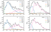 |
Fig. 2. Redshift distribution models, N(z), for the NVSS (top panels) and TGSS catalogs (bottom panels) shown in the range z = [0, 3]. Predictions from the S3 simulator are shown to the left and T-RECS to the right. The thick black histogram in each panel shows the distributions of all sources in the catalog. Histograms with different colors indicate the distribution of each object type identified by the labels. |
Both NVSS and TGSS are composed by different types of sources. The resulting effective bias of the full sample can be defined as
where bi(z) and Ni(z) are the galaxy bias and the redshift distribution of each object type. In this work, we considered six different models for the effective bias b(z), divided into two categories based on whether they are taken from the literature or estimated from the data. The behavior of the various models in function of redshift is shown in Fig. 3 for the NVSS (top panel) and TGSS (bottom panel) case.
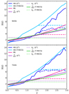 |
Fig. 3. Bias models used in this work as a function of redshift in the range z = [0, 3] for the NVSS (top panel) and TGSS (bottom panel) cases. Curves with different colors and line styles are used for the different combinations of N(z) and galaxy bias models, as indicated in the labels. The values of the free parameter, bg, are listed in Tables 6 and 7 for TGSS and NVSS, respectively. We also consider “truncated” versions of the HB and PB models, in which the value of the bias for each population of sources is kept constant for z ≥ 1.5 (dashed lines). |
The first category of bias prescriptions is based on the halo model (Cooray & Sheth 2002), and they have been proposed in previous studies to describe the auto-correlation function of the radio sources. The “halo bias” (HB) model was presented by Ferramacho et al. (2014) and used by Dolfi et al. (2019) in the NVSS and TGSS auto-correlation studies. It uses the halo model prescription to assign different types of radio sources to halos of different masses and, accordingly, with different biases bi(z). As a consequence, looking at Eq. (11) the HB model depends on the assumed N(z), either S3 or T-RECS. Both models predict that the bias steadily increases with the redshift, which is rather nonphysical. Therefore, we also considered a “truncated halo bias” (THB) model in which we set the bias of each source population to remain constant for z ≥ 1.5. The “parametric bias” (PB) model has been proposed by Nusser & Tiwari (2015) to describe the angular power spectrum of NVSS sources. Following Dolfi et al. (2019), we also used the same PB model in combination with both T-RECS and S3 distributions, for the NVSS and TGSS catalogs. As for the HB prescription, we also consider a truncated parametric bias (TPB) version with constant bias for z ≥ 1.5.
The second category of bias models are simpler and are characterized by parameters that are free to best fit the data. “Model 1” assumes that the bias of radio sources evolves with the inverse of the linear growth factor: b(z) = bg/D(z), where bg is the free parameter of the model and D(z) has been computed using the Colossus8 toolkit assuming the reference PlanckΛCDM cosmology (Planck Collaboration VI 2020). Bias “model 2”, instead, assumes a constant bias b(z) = bg. The bg values used in Fig. 3 are those that best fit the data (see Sect. 6 and Tables 6 and 7).
To summarize, the ingredients used to model the auto- and the cross-angular spectra are: the reference ΛCDM background cosmology Planck Collaboration VI (2020), a HALOFIT-based matter power spectrum P(k, z) model generated with CAMB, a model for the redshift distribution of radio sources, N(z), and for their bias, b(z). We stress that, these two quantities take into account the composite nature of the sample by considering the bi(z) and Ni(z) functions of each radio type (see Eq. (11)). We used these quantities to model the angular spectra in Eqs. (7) and (9) since the CAMB version used in this work does not offer the possibility to include the contribution of each population separately.
For reasons that will be justified in Sect. 4.2, in our analysis we only considered multipoles ℓ ≥ 11. As a result the effect of peculiar motions, which boosts the clustering amplitude on large angular scales, is negligible, as we verified by including this effect in one of our model spectra (the one that adopts the TPB+S3 model combination). In this case, which we regard as representative, the boosting effect at ℓ ≃ 10 is 0.7%. A second benefit is the possibility of using the Limber approximation. Its impact has been evaluated for the same TPB+S3 model. The difference between angular spectra evaluated using the Limber approximation and through a complete 2D integral is less than 0.2% at ℓ ≃ 10, decreasing thereafter. Finally, we also included the effect of the lensing magnification bias, which systematically modifies the number of objects above the flux threshold of the catalog. The magnitude of the effect depends on the effective slope  of the luminosity function of radio sources in the faint end. It can be estimated by combining the slopes of the luminosity functions of the individual objects’ type, as (Dolfi et al. 2019)
where j runs over the redshift bins, i identifies the object type, Ni(z) its redshift distribution, and α(i, j) the faint-end slope of each luminosity function type, i, at the redshift j. The sensitivity of our results to lensing magnification bias will be assessed in Sect. 7.3.
4. Estimated angular power spectra
We measured the auto- and cross-correlation of the CMB lensing convergence, κ, and galaxy counts, g, in harmonic space, using the angular pseudo-power spectrum formalism.
By expanding a generic field, X, defined on a pixelized 2D map over a fraction of the sky in spherical harmonics, we get
where the sum runs over the pixels. The weight function  quantifies the effect of the mask described in Sect. 2. It is set to zero in unobserved sky areas or in pixels in which the signal-to-noise is below some threshold.
Under the assumption of statistical isotropy, the pseudo angular power spectrum of two fields X, Y = {κ, g} can be estimated from the measured harmonic coefficients as
When X = Y we get the auto-angular power spectrum, while if they differ the expression provides the cross-angular power spectrum. The actual power spectrum is derived from the measured pseudo-spectrum as (Hivon et al. 2002; Polenta et al. 2005)
In the above equation,  is an estimate of the noise angular power spectrum, which is nonzero only when X = Y. The matrix
  accounts for the power-loss and mode-mode coupling due to incomplete sky coverage and survey footprint. It is defined as
Here  is the cross-power spectrum of the masks, which is defined as
where  and
and  are the spherical harmonic coefficients of the masks of the analyzed fields.
Under the assumption that κ and g are both random variables, we can represent the joint covariance matrix of the angular auto-gg and cross-κg spectra as
in which each block can be written as
![$$ \begin{aligned} \nonumber \mathrm{Cov}^{Xg,\, X^{\prime }g}_{\ell \ell ^{\prime }}&= \frac{\delta _{\ell \ell ^{\prime }}}{(2\ell +1)\,f^{Xg,\,X^{\prime }g}_{\rm sky}} \left[\left({C}^{XX^{\prime }}_\ell +{N}^{XX^{\prime }}_\ell \right)\left({C}^{gg}_{\ell ^{\prime }}+{N}^{gg}_{\ell ^{\prime }}\right) \right.\\&\quad + \left.\left({C}^{Xg}_\ell +{N}^{Xg}_\ell \right)\left({C}^{gX^{\prime }}_{\ell ^{\prime }}+{N}^{gX^{\prime }}_{\ell ^{\prime }}\right)\right]. \ \end{aligned} $$](/articles/aa/full_html/2023/03/aa44799-22/aa44799-22-eq37.gif)
In the above Eq., X and X′ can be both κ and g, Cℓs are the theoretical angular power spectra corresponding to the fiducial model, while the sky fractions are defined as  and the different
  values are given in Sect. 2.
In our analysis, we binned the estimated spectra  within equally spaced linear bins, Δℓ. Consequently, the elements of the covariance matrix will also consist of Δℓ-binned quantities.
The main reason for binning the spectra is to reduce the multipole covariance induced by the mask hence decreasing the amplitude of the off-diagonal elements. In our main analysis, we set the bin size to Δℓ = 30. This choice guarantees that the covariance matrix is well approximated by a diagonal Gaussian model, as we show in Appendix B. In the same appendix, using Monte Carlo simulations, we also verified that our pipeline for power spectrum estimation is unbiased, namely it does not introduce spurious correlations and it is able to recover a known input power spectrum.
4.1. Angular auto-power spectrum of radio sources
To measure the angular power spectrum of the radio sources,  , we used the estimator defined in Eq. (14) with X = Y = g, which also corrects for a noise term. For the auto-spectrum it is given by the sum of the Poisson noise
  (
( being the mean number of radio sources per pixel) and the spurious contribution due to multiple components of a single source counted as individual sources. These noise terms were estimated by Dolfi et al. (2019) for the TGSS and NVSS samples used in their analysis.
We reassessed these corrections by requiring that the auto-spectrum should be consistent with zero at high ℓ where the noise term is expected to be dominant. We find that the original Dolfi et al. (2019) correction is adequate for the TGSS case and it is Ngg = 8.86 × 10⁻⁵. On the other hand, for the NVSS case it provides an over correction and, as a consequence, the angular auto-spectrum takes negative values at high multipoles. For this reason, we estimate the correction from the data by treating the noise term Ngg as a free parameter in the best fitting procedure described in Appendix A. With this method, the best fitting noise terms listed in Table A.1 depend (only mildly) on the theoretical model adopted for the angular power spectrum.
The binned angular power spectra measured in the range ℓ = [11, 130] for the reference NVSS and TGSS samples are shown in Fig. 4. We discard all multipoles below ℓ = 10 from our analysis. There are various reasons for this conservative choice. First of all, the fact that in NVSS survey the flux sensitivity is modulated by the Galactic latitude (Smith et al. 2007) and can generate spurious correlation on large angular scales. Moreover, the anomalously large amplitude of the TGSS auto-spectrum on these scales has been interpreted as a manifestation of systematic effects (Dolfi et al. 2019; Tiwari et al. 2019). Finally, these are the scales at which systematic effects, related to Galactic emission and absorption processes, can potentially affect both the radio sources and the lensing signal and, therefore, their angular cross-correlation. The choice of ℓmax = 130 is due to the fact that, for greater multipoles, the auto-spectra are dominated by shot noise. We also used the same ℓ-cuts for TGSS. Error bars in the plot represent the 1σ uncertainties computed with Eq. (18), for X = X′=g. We note that the binning scheme used for this plot is Δℓ = 10 to ease the comparison with the auto-spectra estimated by Dolfi et al. (2019). This outcome confirms their result and the power excess in the TGSS sample for ℓ ≤ 20 − 30.
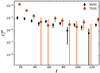 |
Fig. 4. Binned angular power spectra of NVSS (black diamonds) and TGSS (red dots) sources in the range ℓ = [11, 130]. The size of the bins is Δℓ = 10. Error bars are 1σ Gaussian uncertainties from Eq. (18). Power spectra are corrected for both shot noise and multiple component contributions (see text for details). |
4.2. Angular cross-power spectrum of CMB lensing convergence and radio sources
The cross-power spectrum,  , is estimated using Eq. (14) with X = κ and Y = g. We estimated the cross-spectrum in the multipole range ℓ = [11, 310] and in bins Δℓ = 30. The ℓ range is wider with respect to the auto-spectrum case. Its upper value ℓmax = 310 is set to minimize the impact of nonlinear effect that would break the Gaussian hypothesis adopted to model the covariance matrix. To estimate ℓmax, we compared the theoretical angular cross-spectrum obtained assuming a linear matter power spectrum with that obtained using the HALOFIT approximation and search for the ℓ value at which the difference between linear and nonlinear predictions reach 10%. As we considered three different HALOFIT models, we obtained three values for ℓmax = 310, 325, 350 and opted for the most conservative one. We also notice that the gain in signal-to-noise is quite low above this multipole.
The estimated CMB lensing convergence-radio source cross-spectrum is shown in Fig. 5 for the NVSS and TGSS cases. Error bars represent 1σ uncertainties obtained with Eq. (18), where X = X′=κ. Unlike for the auto-spectrum case, we now find a good match between the two samples down to the smallest multipole explored, that is, we do not find evidence of a power excess in the spectrum of TGSS sources anymore. This result strongly suggests that the power excess in the TGSS auto-spectrum is not genuine but likely originates from uncorrected systematic effects in the observations. Hence, it also corroborates the suggestion made by Tiwari et al. (2019) that the excess power in the TGSS catalog probably originates from systematic effects in the flux calibration. Moreover, this result clearly illustrates the effectiveness of the cross-correlation as a tool to identify and reduce the impact of any systematic effect that does not correlate with the LSS.
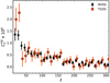 |
Fig. 5. Cross-angular power spectra of the NVSS catalog (black diamonds) and TGSS catalog (red dots) with CMB lensing convergence in the range ℓ = [11, 310] measured in bins Δℓ = 10. Error bars are the 1σ Gaussian uncertainties from Eq. (18). |
We note that for both radio catalogs, we report a high-significance detection of the cross-correlation with Planck CMB lensing. To assess the significance of this detection, we compared our results with the null hypothesis, namely the probability that no correlation is found between the CMB lensing convergence field and the radio galaxies distribution. We quantified this probability by estimating  :
:
where  is the estimated power spectrum and
  is the covariance matrix associated with the cross-power spectrum only. We obtain the significance in unit of sigma as the square root of the difference between the null hypothesis and the χ2 of the best-fit model, namely:
  . The best-fit theoretical model is the one obtained considering TPB + T-RECS as it is reported in Tables 2 and 4, respectively, for TGSS and NVSS (see Sect. 5 for more detailed analysis and notation). We found a detection significance of 22σ for the NVSS catalog, compatible with Planck Collaboration XVII (2014), and of 12σ for TGSS.
χ2 analysis results for TGSS cross-spectrum and PTE values.
5. Testing radio sources b(z) and N(z) models
We now compare the angular spectra estimated in the previous section with model predictions obtained using different prescriptions for the redshift distribution and for galaxy bias of the radio sources. Some of these prescriptions are taken from the literature and some have been proposed here for the first time, as pointed out in Sect. 3. We performed two different analyses. The first one involves cross-spectra only. The second one is a joint analysis that includes both cross- and auto-spectra. In both cases we used a χ2 statistics to assess the relative goodness of the proposed models:
where the sum runs over the multipole bins,  is the data vector, Cℓ represents the model and Covℓℓ′ is the covariance matrix. For all χ2 analyses we consider bins Δℓ = 30. To evaluate the consistency of the data vector with the model predictions we provide, along with the reduced χ2, the probability-to-exceed (PTE), that is, the probability of obtaining a χ2 value higher than what we actually measure: PTE = 1 − P(< χ2).
In the first χ2 analysis, the data vector is the estimated cross-spectrum defined in Sect. 4.2
 , the model power spectrum is that of Sect. 3
 and we use the Gaussian diagonal covariance matrix of Eq. (18) where X = X′=κ. For the cross-spectrum we consider ten equally spaced bins in the range ℓ = [11, 310]. As a result, we have a covariance matrix of 10 × 10 elements.
The second analysis includes both the κg cross- and the gg auto-spectra. The latter has been estimated in Sect. 4.1. Since we use a Δℓ = 30 binning scheme, it contributes with additional 4 elements to the data vector that now contains 14 elements. The size of the corresponding covariance matrix is then 14 × 14. Our results for the two analysis are further discussed in the following sections.
5.1. Cross-angular power spectrum results
In the two panels of Fig. 6, we compare the measured TGSS-CMB lensing convergence cross-spectrum with predictions obtained from different N(z) and b(z) models, as summarized by the labels. We distinguish two sets of models. Those obtained assuming the N(z) simulated by S3 (top panel) and those obtained using the N(z) simulated by T-RECS (bottom). Error bars represent 1σ Gaussian uncertainties. Since the covariance matrix is computed for each model, they are model dependent. However, as we verified, the dependence is weak and we plot those obtained with the TPB bias model for reference.
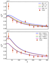 |
Fig. 6. κg cross-spectrum analysis for the TGSS sample. Red dots represent the estimated power spectrum while error bars correspond to 1σ Gaussian uncertainties. Curves with different colors are theoretical predictions of different b(z)+N(z) combinations, as specified by the labels. Top panel: models that use the S3N(z). Bottom panel: models that use the T-RECS N(z) predictions. |
The results of the χ2 analysis are reported in Table 2, where we list the values of the reduced χ2, which have been obtained for ten degrees of freedom (d.o.f.), together with the corresponding PTE values. The visual inspection of Fig. 6 reveals several interesting features. First, for a fixed bias model (i.e., the PB and TPB cases), the amplitude of the cross-spectrum obtained in the T-RECS case is systematically larger than in the S3 case. This reflects the different redshift distributions and biasing properties of the radio sources in the two N(z) models. According to T-RECS, TGSS is dominated by a population of bright FRII sources with an effective bias that rapidly increases with the redshift. In the S3 case, the fraction of FRII sources is smaller.
Their distribution extends to higher redshifts and at moderate redshift the sample is dominated by a comparatively fainter FRI + SFG population whose bias increases slowly with the redshift. A second remarkable feature is the impossibility, for all S3 models, to match the amplitude of the cross-spectrum in the first bin. A match that is obtained when using the T-RECS N(z) and the HB and THB bias models. Again, this reflects the fact that the population of nearby objects, which most contribute to the amplitude of the spectrum on large angular scales, in the S3 case is dominated by object that are less biased than their T-RECS counterparts. We should also notice that while T-RECS + HB and T-RECS + THB fit the amplitude of the first bin, they fail to match the cross-spectrum in most of the other bins.
Table 2 shows that these are in fact the models that provide the worst fit to the data. All the other models provide an acceptable fit to the data for ℓ > 40. The PB and TPB ones are those that perform better in both the T-RECS and S3 cases. Following the interpretation given by Tiwari et al. (2019), who argue that the power excess at ℓ ≤ 30 − 40 in the TGSS catalog is likely due to systematic effects, we replicated the analysis discussed above excluding the first ℓ bin (i.e., considering the range of multipoles ℓ = [41, 310]). Regardless, we find χ2 values that are consistent with those obtained using the baseline multipole range, owing to the limited constraining power of the TGSS sample. The χ2 results for ℓ > 40 are summarized in Table 3.
The χ2 analysis of the NVSS sample (results shown in Fig. 7) provides similar results (see Table 4). All models but HB and THB with T-RECS number counts fail to match the amplitude of the cross-spectrum in the first ℓ bin. The analysis also confirms that the PB and TPB bias models perform better especially when coupled to the T-RECS N(z) redshift distribution model. However, they generally provide worse PTE values than in the TGSS case, reflecting the smaller uncertainties of the measured NVSS κg cross-spectrum.
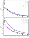 |
Fig. 7. Same as Fig. 6 but for the NVSS κg cross-spectrum analysis. The estimated power spectrum is shown with black diamonds. Error bars represent 1σ Gaussian uncertainties. |
Reduced χ2 for the NVSS cross-spectrum alone and PTE.
To summarize, the results of the cross-spectra analyses favor the PB and TPB bias models over the HB and THB ones, with a mild preference for the T-RECS N(z) model over S3 for the NVSS case. However, the PB and TPB models do not match the power amplitude on large angular scales. The significance of the mismatch is not high (about 2.4σ) but it is seen in both samples and, if confirmed, could indicate a genuine large-scale excess power in the radio sources.
5.2. Combined cross- and auto-angular power spectra results
The analysis of the κg cross-spectrum can only constrain the combination b(z)+N(z). Since this degeneracy is potentially broken by combining the cross- and the auto-spectrum analysis, we perform a joint analysis using both. Considering that there is significant evidence that the auto-spectrum of the TGSS catalog is affected by systematic errors, we restrict our joint analysis to the NVSS sample only.
As explained in Sect. 4.1, we estimated the noise correction to the NVSS auto-spectrum, Ngg, from the data, since values from literature overestimate it. Also for the joint analysis, in the modeled auto-spectrum we include the noise term, Ngg, to account for both Poisson noise and spurious contribution from misidentified multiple sources. We treat Ngg as a free parameter and estimate its value by minimizing the χ2(Ngg) function. The details of the procedure are described in Appendix A where we provide the best-fit Ngg values in Table A.1 and also compare them with those obtained by using only the auto-spectrum. We summarize the results of the χ2 joint analysis in Table 5, where we list the minimum (with respect to Ngg) reduced χ2 values along with the corresponding PTE for all N(z) and b(z) models. We note that in this case the number of d.o.f. is 13 (i.e., 14 elements of the data vector minus one fitted parameter). Results of the joint analysis confirm those obtained using the cross-spectrum only. Bias models HB and THB are now even more strongly disfavored. The mild preference for using T-RECS in combination with PB and TPB with respect of using S3 is also confirmed.
NVSS joint gg auto- and κg cross-spectrum χ2 analysis.
6. Constraints on the effective bias of radio sources
So far we tested the ability of existing N(z) and b(z) models to fit the observed auto-gg and cross-κg spectra, with no attempt to set constraints on either models. In this section we change strategy and we use the spectra to constrain the effective bias of the radio sources and its evolution, b(z), having assumed a model for their redshift distribution N(z). We do not adopt the alternative strategy of assuming b(z) while leaving N(z) free to vary since the observational constraints of the redshift distribution of the radio galaxies are tighter than those for their bias. In any case, to account for the theoretical uncertainties in the N(z) model we consider both T-RECS and S3 and propagate this difference to the b(z) uncertainty.
We consider the two bias models, dubbed model 1 and model 2, that were introduced in Sect. 3 and depend on one free parameter only, bg. Their simplicity is motivated by the need of minimizing the free parameters of the model since the number of data points in the analysis is limited (10 and 14, in the cross- and joint-spectra analyses, respectively). To estimate bg, we search for the minimum value,  , of the χ2(bg) function evaluated in 500 equally spaced points in the interval [bmin, bmax]. The angular spectrum model is evaluated in each of the 500 points, whereas the covariance matrix is set equal to that of the “fiducial” model, which is provided by the best fit found in Sect. 5. Therefore, we adopt the one based on the TPB bias model and on either the S3 or the T-RECS N(z), depending on which one is used for the angular spectrum model. Following the Gaussian hypothesis, we estimate the 1σ uncertainty of the bg parameter by setting
  .
.
As in the previous section, we first perform the χ2 minimization using the cross-spectrum information only. In this case we consider both the TGSS and the NVSS sample. Then we repeat the procedure using both the cross- and the auto-spectra. In this second case we restrict the analysis to the NVSS case only.
For the TGSS catalog, results are shown in Fig. 8, and the best fitting bias parameters are listed in Table 6. For NVSS, results are instead summarized in Fig. 9 and Table 7.
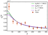 |
Fig. 8. Best-fit κg power spectra models for the TGSS sample (solid and dashed lines) vs. measured (red dots) and their 1σ Gaussian error bars. Different colors and line styles are used for the different redshift distribution models: N(z) from T-RECS (green) and N(z) from S3 (purple). Continuous lines refer to a linearly evolving bias (model 1) while dashed lines to a constant bias (model 2). The best fitting bg values are listed in Table 6. |
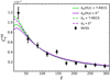 |
Fig. 9. Same as Fig. 8 but considering the NVSS sample. Data are now shown with black diamonds along with their 1σ error bars. Colors and line styles of the model cross-spectra are also the same. Values of the best-fit bg are summarized for the different models in Table 7. |
bg best-fit values obtained by considering TGSS κg alone.
NVSS bias parameter, bg, best-fit values considering κg alone.
The bg values of TGSS are consistent, though somewhat higher than those found for the NVSS sample. This is expected since TGSS objects are typically brighter, and therefore more biased, than the NVSS ones. The fact that the PTE values for TGSS are smaller than for NVSS simply reflects the fact that errors in the measured κg TGSS spectrum are larger than in the NVSS one because of the smaller number of sources. Leaving the bias model free to vary generally improves the quality of the fit and significantly reduces the mismatch between models and data in the first multipole bin.
Moreover, the constant model 2 bias fits the data better than the evolving model 1, irrespective of the N(z) model adopted. In fact, for any given bias model, the two best-fit bg values obtained using either T-RECS or S3 are consistent with each other, indicating that these results are rather insensitive to the N(z) model uncertainty. On the contrary, the bg value is sensitive to the bias model adopted, being systematically larger for model 1 than for model 2.
For the joint analysis, we also considered the four additional data points of the NVSS gg auto-spectrum. One important difference with respect to the cross-spectrum analysis only is the fact that we now minimize the χ2 function with respect to two free parameters: the effective bias bg and the auto-spectrum noise term Ngg. We therefore search for the minimum of the  function. To find the 1σ confidence level of each parameter, we firstly estimate the 2D joint probability function,
  . Then we marginalize over one parameter to obtain the 1D probability function of the other, P1D, and consider its 16th to 84th percentile interval.
The 1D probability distributions for bg obtained for the joint analysis (continuous curves in Fig. 10) are very similar to those obtained from the NVSS cross-spectrum only analysis (dotted curves). The best fitting bg values found in correspondence of the maxima are indicated by a vertical line and listed in Table 8 along with their 1σ errors. In Table 8, we also show the value of the noise term Ngg with its uncertainty and the minimum value of the reduced  along with its PTE. We note that the estimates of Ngg are in agreement with those computed in Appendix A for the bias models taken from the literature. The results of the joint analysis agree with those obtained from the cross-spectrum only and confirm their weak sensitivity to the choice of the N(z) model. However, unlike in the joint analysis presented in Sect. 5.2, the addition of the auto-spectrum does change the results since the preference for bias model 2 over model 1, which was rather weak in the κg only analysis, it is now significantly stronger. The reason for this is clearly seen in Fig. 11 in which we compare both the NVSS κg (top panels) and gg (bottom panels) measured spectra (black diamonds) with the different best fitting models (continuous solid and dashed curves). Shaded areas represent the 2σ uncertainty interval of the estimated bg parameter. The two model cross-spectra, whose amplitude scales as bg, provide similar predictions. This is not the case for the auto-spectra for which the two models, whose amplitudes scale as
  , significantly depart from each other at small ℓ values. The preference of bias model 2 over bias model 1 largely stems from this different behavior. The quality of the fit has also improved, especially for the bias model 2 case, with respect to the κg only analysis as indicated by the larger PTE values.
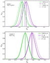 |
Fig. 10. Marginalized 1D probability distributions, P1D, of bg for different bias models. The continuous curves show P1D for model 1 (constant bias) and model 2 (linearly growing bias), obtained from the joint NVSS gg and κg power spectrum analysis. All curves are normalized so that P1D = 1 at the maximum. Different colors indicate the different N(z) models and match those used in Fig. 9. Dotted curves are drawn for comparison and show the P1D from the NVSS cross-spectrum-only analysis. They are labeled CA to further distinguish them from those obtained from the joint analysis, labeled JA. |
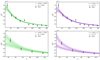 |
Fig. 11. Model vs. measured NVSS κg (top panels) and gg (bottom panels) angular power spectra. The measured cross-spectra (top panels) are the same as in the previous plots. Error bars represent 1σ Gaussian uncertainties. The curves show model predictions. They are surrounded by shaded areas that represent the 2σ uncertainty interval of the best fitting bg values. The green color in the left panels indicates models that adopt the T-RECS N(z) prescription. The purple color flags the adoption of the S3 model in the right panels. Continuous and dashed lines are used for bias model 1 and model 2, respectively. All best fitting bg values are listed in Table 8. |
Best-fit values for the NVSS bias parameter, bg, and for the shot-noise term, Ngg, obtained from the joint κg and gg power spectra analysis.
7. Robustness tests
In this section we present a number of tests designed to assess the robustness of the results of the cross-spectrum analyses presented so far. We focused on the cross-spectra results only for two reasons. First, constraints on the N(z) and bias models largely come from this statistics alone. Secondly, similar robustness tests have been performed, successfully, on the TGSS and NVSS auto-spectra by Dolfi et al. (2019). These tests are designed to assess the impact of possible observational systematic effects on either the radio catalogs or the convergence maps, or both.
7.1. Robustness to residual astrophysical foreground contamination
To minimize the impact of foreground Galactic emission and that of confusion associated with high stellar density, in Sect. 2 we masked out the sky area that is close to the Galactic plane, both in the CMB lensing convergence map and in the TGSS and NVSS source catalogs.
To assess the robustness of our analysis to the choice of the mask, we repeated the cross-correlation analysis using two more aggressive Galactic cuts to exclude regions with |b|< 30° and |b|< 40° in all maps. As a result, the sky fraction considered in the analysis decreases to  (0.41) and
  (0.30) for the cross-correlation with NVSS (TGSS). We compared the results with those obtained with the baseline sky masks of Sect. 2. In Fig. 12 we show the difference between the new and the baseline cross-spectra,
  , in units of the Gaussian error
  from Eq. (18) estimated considering the TPB bias model, the T-RECS model for N(z) and using the most aggressive mask. The upper and bottom panels show the results for the NVSS and TGSS cross-spectra, respectively. Horizontal dashed lines are drawn at the 1σ level value for reference. For both mask choices and for both radio source catalogs, the residuals show no significant trends with ℓ or fsky and their amplitude oscillates within the dashed lines. We conclude that the results of our analysis, obtained with the baseline mask, are robust to possible systematic effects associated with Galactic foreground contamination.
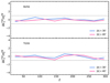 |
Fig. 12. Residuals, |

Besides Galactic foregrounds, another possible source of contamination is represented by extragalactic point sources. Extragalactic objects are expected to trace the same LSS as the radio sources. Moreover, since they follow a highly non-Gaussian distribution, they could bias the CMB lensing maps since the lensing reconstruction relies on the non-Gaussian nature of the lensed CMB. In particular, contamination from extragalactic point sources can even correlate with the radio sources distribution we are investigating. As a result, they can potentially bias the cross-correlation spectrum. To assess their impact on our cross-correlation analysis, we considered a different lensing reconstruction, that obtained from polarization CMB data. At present, the extragalactic contamination in polarization is not robustly quantified, but it is expected to be less of a problem because of the comparative lower fraction of polarized sources (Smith et al. 2009). While the Planck lensing is mostly dominated by the CMB temperature information, an independent lensing map has been generated and only accounts for CMB polarization data (Planck Collaboration VIII 2020). In Fig. 13, we compare the angular power spectra estimated by cross-correlating NVSS and TGSS sources with Planck lensing reconstructions obtained from CMB temperature-only data (TT), polarization-only data (PP) and their MV combination, the last being the baseline lensing map we used in this work. The polarization reconstruction is significantly noisier, an aspect that motivated us to use wider multipole bins Δℓ = 50 for this comparison, instead of the baseline one Δℓ = 30. Figure 13 shows that different lensing reconstructions provide compatible results. Hence, we conclude that systematic errors induced by extragalactic sources contamination are well within the expected statistical uncertainties of our analysis.
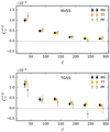 |
Fig. 13. Cross-angular power spectra for NVSS (top) and TGSS (bottom) with different Planck CMB lensing reconstructions obtained with temperature-only data (TT), polarization-only data (PP), and their MV combination. To estimate the spectra, we used the baseline mask and a multipole bin size Δℓ = 50. |
7.2. Robustness to radio flux cut
As discussed in Sect. 1, wide radio surveys are prone to large-scale variations in the flux calibration. This effect can modulate the completeness of the sample and generate spurious signals in the angular spectra at low multipoles. The amplitude of the effect is expected to be larger at fainter fluxes, where the completeness of the catalog drops. To assess the potential impact of this effect we followed Dolfi et al. (2019) and select subsamples of NVSS and TGSS radio sources using different (lower) flux cuts Smin that we cross-correlate with the CMB convergence maps.
For the NVSS case we gradually increased the flux cut from the baseline value Smin = 10 mJy up to 20, 50, and 100 mJy. The results are shown in the top panel of Fig. 14, in which we plot the difference of the κg cross-correlation spectra with respect to the baseline case, in units of the 1σ Gaussian error. This error is the same as the baseline Gaussian error in which, however, the Poisson noise term is the one of the sub-catalog selected at the new Smin value. The normalized residuals are confined within the 1σ uncertainty strip, which indicates that the results of the NVSS cross-correlation analysis are robust. Since a similar robustness was found for the NVSS auto-correlation analysis (Dolfi et al. 2019), we conclude that also the joint analysis is robust to cutting the sample at Smin ≥ 10 mJy.
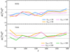 |
Fig. 14. Residuals, |


We repeated the same analysis for the TGSS case and find similar results. Here we considered cuts at Smin = 50 and 100 mJy that are less aggressive than the baseline case (200 mJy) as well as a more conservative one for which Smin = 300 mJy. As shown in Fig. 14, residuals are generally below the 1σ Gaussian error, which indicates that the TGSS cross-correlation analysis is robust to the choice of Smin.
Finally, we also checked that results are insensitive to the choice of the upper flux cut, Smax, as in the case of the auto-correlation analysis (Dolfi et al. 2019). We consider two different values, Smax = 3000, 5000 mJy. The residuals, computed with respect to the baseline value Smax = 1000 mJy, show no significant trend with the value of multipoles or flux cuts. In particular, for TGSS, considering a more conservative flux cut at Smax = 1000 mJy with respect to Smax = 5000 mJy leads to an increase in the error bars on the order of 8%. We conclude that the cross-correlation is also robust to changes in Smax.
7.3. Robustness to lensing magnification bias modeling
In the angular spectra models introduced in Sect. 3, we accounted also for the lensing magnification bias, which has an impact on large angular scales. The effect is fully quantified by a single parameter  , which represents the effective slope of the faint end luminosity function of the radio sources. It is defined as the weighted mean of the individual luminosity function slopes of the various objects’ types (Eq. (12)). So far, we have used
  , that is, we set this value equal to that of Dolfi et al. (2019) originally evaluated for TGSS and assuming a S3N(z) model. However, the value of the
  depends on the type of objects included in the catalog and on their individual redshift distributions. To investigate the sensitivity of our results to the choice of
  , we repeated the cross-correlation analysis for both the TGSS and NVSS cases using a T-RECS N(z) model and assuming a TPB bias while the
  parameter is free to vary. Then, we search for the minimum of the
  function evaluated in 600 equally spaced points in the range
 ![$ \tilde{\alpha} = [-1.0,2.0] $](/articles/aa/full_html/2023/03/aa44799-22/aa44799-22-eq82.gif) . The corresponding 1D probability distribution functions for
. The corresponding 1D probability distribution functions for  are shown in Fig. 15 and compared with the reference value
  (cyan vertical line). The two probability functions peak at two different
  values, confirming that
  does depend on the catalog used. Moreover, the difference between the TGSS best-fit value
  and that of Dolfi et al. (2019) quantifies the sensitivity to the N(z) model. That said, the differences between the reference and the best-fit
  values is within the variance of the two distributions, both close to Gaussian. We therefore conclude that our analysis is robust also to the choice of
  .
.
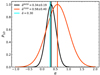 |
Fig. 15. Probability distribution functions for the magnification bias parameter, |


8. Discussion and conclusions
In this work we have investigated the cross-correlation between wide surveys of extragalactic radio sources, namely TGSS and NVSS, and CMB lensing. Both are tracers of the underlying mass distribution and potentially affected by different and supposedly uncorrelated observational systematic uncertainties. Their cross-correlation analysis should then be insensitive to the systematic errors that might instead affect the auto-correlation measurements. Moreover, a joint analysis that combines auto- and cross-correlation statistics is able to break, at least in part, the degeneracy between the bias and the redshift distribution of the tracers, two quantities that are weakly constrained in the case of wide radio surveys.
The main results of our analysis are the following:
-
We confirm an excess clustering power of the TGSS sample over the one from NVSS at large angular scales. This excess has been detected with high statistical significance in previous analyses in the multipole range ℓ ≤ 40 and regarded as a spurious feature that should be attributed to some observational or instrumental effect (Tiwari et al. 2019). When the same flux cuts, sky areas, and ℓ-binning are adopted, we reproduce the results of Dolfi et al. (2019), which constitutes a consistency test for our analysis pipeline.
-
The cross-correlation spectrum of the NVSS-CMB lensing convergence is in good agreement with the TGSS-CMB lensing convergence in the range ℓ = [11, 310]. The choice of excluding multipoles ℓ < 11 is conservative and motivated by the known dependence of the flux sensitivity on the Galactic latitude for the NVSS sources, which could generate spurious power on large angular scales (Smith et al. 2007). The upper limit ℓ = 310 was set to reduce the impact of nonlinear effects in the matter power spectrum and, thus, to minimize deviations from the Gaussian statistics that we assumed in order to estimate the covariance matrix and perform the χ2 analysis. The large mismatch seen in the TGSS and NVSS auto-spectra at ℓ < 40 is not observed in the cross-spectra, which are instead in good agreement. Although this result does not clarify the origin of the large-scale power excess detected in the TGSS auto-spectrum, it does support the hypothesis that it is not genuine but originates from observational systematics errors that could not be identified and corrected for. The absence of this excess in the cross-correlation validates the hypothesis that possible observational biases in the CMB lensing maps do not correlate with those that affect the TGSS catalog. Moreover, it confirms that cross-correlation analyses between CMB lensing and catalogs of extragalactic objects are less prone to observational systematic errors and, therefore, can safely be exploited to make inferences on the nature, redshift distribution, and clustering properties of the radio sources. We also stress that while the NVSS-CMB lensing cross-correlation signal has already been measured (Planck Collaboration XVII 2014), this is the first time that such a cross-correlation signal has been detected using TGSS, which is a catalog that contains a different mixture of radio sources.
-
None of the combinations of the b(z)+N(z) models proposed to fit the auto-power spectrum of the NVSS and TGSS sources, and that we implemented in our analysis, are also able to fit the observed κg cross-spectrum over the full ℓ range. In this work we used the two main existing extragalactic radio simulations publicly available, T-RECS and S3, to model the redshift distribution, N(z), of the radio sources in the TGSS and NVSS catalogs. We did not consider their associated b(z) model, which basically reflects the bias of the dark matter halo host extracted from the parent N-body. Instead, we examined two bias models used in previous clustering analyses of the TGSS and NVSS objects (see Nusser & Tiwari 2015; Tiwari & Nusser 2016; Bengaly et al. 2018; Dolfi et al. 2019). The first one, dubbed HB, relies on the halo model applied to all types of radio sources in the T-RECS and S3 simulations (Ferramacho et al. 2014). The second one, PB, relies on the physical model of Nusser & Tiwari (2015) and assumes that only one galaxy can be hosted in a halo. At low redshifts, direct observations provide some constraint on the bias of the various types of radio sources (i.e., Magliocchetti et al. 2017; Hale et al. 2018). On the contrary, at high redshifts the bias of the radio sources largely relies on theoretical assumptions. Both HB and PB predict that the bias steadily (and rapidly) increases with redshift, which is somewhat nonphysical. For this reason, we also considered truncated versions of both models in which the bias amplitude of each radio source population is kept constant for z ≥ 1.5. The choice of this redshift value is quite arbitrary. However, we verified that it has little impact on the results, which are quite insensitive to the choice of the truncation redshift.
-
To quantify the agreement between model and data, we performed a χ2 analysis. To model the angular spectra, we assumed a flat ΛCDM Planck cosmology (Planck Collaboration VIII 2020) and the N(z) and b(z) models described above. The comparison was done in bins of Δℓ = 30 as a compromise between the need to minimize the loss of information due to data compression and that of reducing the covariance among different bins. The latter requirement allowed us to use an analytic diagonal Gaussian approximation to estimate the covariance matrix. The goodness of the Gaussian hypothesis was checked by comparing its results with those obtained by repeating the χ2 analysis using a numerical covariance matrix estimated with the Jackknife (JK) resampling method (Appendix B.1).
-
The results of the χ2 analysis indicate that no N(z) and b(z) model combination succeeds in fitting the cross-spectrum over the full multipole range. Most of the considered models provide a good fit to the data over much of the multipole range, except in the first bin [11, 41] and at ℓ ∼ 150, where they underpredict the amplitude of the cross-power spectrum. This is true for both the TGSS and NVSS catalogs. The power peak at ℓ ∼ 150 is a peculiar feature that has no counterpart in the auto-spectra, which are dominated by shot noise at these multipoles. The excess power in the first ℓ bin, [11, 41], is more striking. A similar excess is also seen in the NVSS auto-spectrum on the same scale, as shown by Dolfi et al. (2019), when it is compared to the HB + S3 model. We found that not only does HB + S3 fail to match the cross-spectrum on the same scales, but other model combinations (PB + S3 and PB + T-RECS) underpredict the NVSS-CMB and TGSS–CMB lensing cross-power on large angular scales. Indeed, the only model combination that fits the angular cross-spectra in the first bin is the HB + T-RECS. The reason for this is related to the rapid evolution of the bias with redshift, which boosts the clustering amplitude of the objects at z < 1.5, since similar results are also obtained with the TPB and THB models, in which the bias of each source population is fixed to be constant beyond z = 1.5. On the other hand, the HB + T-RECS model combination consistently overpredicts the power amplitude at all ℓ > 41, except for the bin centered at ℓ ∼ 150, and provides a much worse fit to the data than the other models, as indicated by the PTE values.
-
When the same bias model is assumed (as in the PB or TPB cases), the κg model is rather insensitive to the choice of N(z). This robustness of the CMB lensing cross-correlation to the N(z) model uncertainties is a key feature that allows us to break the degeneracy between b(z) and N(z) when combined with auto-correlation measurements, as recently also pointed out by Alonso et al. (2021). We therefore performed a joint auto- and cross-correlation analysis using the CMB lensing and the NVSS catalog only. Unfortunately, the limited signal-to-noise of the auto-spectrum is not enough to further discriminate between the various combinations of b(z) and N(z) models. The analysis confirms that none of these combinations succeeds in fitting the auto- and cross-angular spectra on both large and small scales.
-
Intriguingly, a power excess at ℓ < 41 has also recently been detected in the auto-spectrum of the radio sources in the Rapid ASKAP Continuum Survey (RACS) catalog by Bahr-Kalus et al. (2022), an excess that no effective bias model combined with either S3 or T-RECS redshift distributions is able to match. Suspecting a spurious origin of the excess, Bahr-Kalus et al. (2022) compared the results obtained when including or excluding multipoles ℓ < 41 and find that in the latter case the minimum reduced χ2 decreases by a factor of 3-10, depending on the model combination. When we repeated the same exercise and removed the first ℓ bin from our cross- and joint-angular spectra analyses, we also found that the reduced χ2 value decreases, but only by 30-60%, which hardly indicates a spurious origin of this large-scale angular power.
-
We checked the robustness of our results to a number of potential sources of systematic errors and find that they do not change when different flux cuts are used to select the radio samples or when different geometry masks are considered to account for the impact of Galactic foreground. The CMB lensing signal is also prone to potential biases. Therefore, we checked the sensitivity of our results to different Planck CMB lensing reconstructions as well as to the magnification bias modeling and find no significant effect. Moreover, we cross-correlated the radio source data maps with Planck CMB lensing simulations that include realistic reconstruction noise and we recovered a null mean cross-spectrum, thus confirming that possible spurious signals in the radio source maps do not correlate with lensing (see Appendix B.2). Finally, the results of our χ2 analysis are potentially sensitive to the Gaussian hypothesis, which we used to generate the covariance matrix of the auto- and cross-spectra, and to the choice of the ℓ-binning. These tests, which are described in Appendix B, also confirm the robustness of our results.
-
As none of the considered b(z)+N(z) models can successfully fit the cross-spectra, and given the robustness of the model prediction to the uncertainties in the composition and redshift distribution of the radio sources, we repeated the analysis with a fixed N(z) model (either T-RECS or S3) and let a bias parameter free to vary. Specifically, we explored two simple bias models commonly used in the clustering analyses of the radio sources (see also Alonso et al. 2021; Bahr-Kalus et al. 2022): a constant bias and a bias that evolves with the inverse of the linear growth factor, D(z)−1. Both models depend on a single free parameter, bg, the effective bias of the sample at z = 0. Leaving the bias free to vary generally reduces, but does not eliminate, the mismatch between the model and the measured cross-spectra in the first redshift bin, though it does not improve the quality of the fit in correspondence to the power peak at ℓ ∼ 150. The constant bias model outperforms the more physically motivated redshift evolving one for both choices of N(z) and for both the NVSS and TGSS cross-spectra.
-
Focusing on the NVSS case, we find that the best-fit bg values obtained for the non-evolving bias model (2.53 and 2.79 for the T-RECS and S3 case, respectively) are systematically larger than those of the D−1(z) evolving model (1.64 and 1.73). The difference is significant compared to the typical 1σ uncertainty of 5% on bg. Since bg represents the effective bias of the NVSS sample at z = 0, this large value would imply the presence of a local population of radio sources that are significantly biased with respect to the mass density field. This seems to be in contradiction with the evidence that at low redshift the NVSS sample is dominated by low-biased SFGs and FRI sources. Interestingly, a similar result has been found in the auto-correlation analysis of the RACS sample (Bahr-Kalus et al. 2022). The RACS sample, like the NVSS one, is locally dominated by SFGs and FRI sources. However, the constant bias best fitting model requires a high linear bias parameter, 2.41 or 3.24, depending on the N(z) model adopted. Evidently, in their case as well as in ours, a large bg value is required to fit the power on large angular scales that is mainly contributed by the local LSS. Invoking a bias that increases with redshift, either linearly or exponentially, significantly reduces the best-fit bg values, as in our case. However, and unlike our case, the adoption of an evolving bias in the RACS analysis either improves or does not significantly modify the quality of the fit.
-
We ascribe the preference for a constant bias model with a large bg parameter to the attempt to fit the large-scale power at ℓ < 40. Interestingly, Bahr-Kalus et al. (2022) also find a large power excess in the auto-spectrum for ℓ < 40, an interval of multipoles that they needed to exclude from the analysis to obtain reasonably good fit to the data. When they cross-correlated the positions of the RACS sources with the CMB temperature map, this large-scale power excess, which they interpret as spuriously generated by observational systematics, is largely removed, as it should be in our cross-correlation analysis. For this reason, we are very cautious in dismissing the cross-power in the first multipole bin as non-genuine. We repeated the same analysis for the TGSS–CMB lensing cross-spectra. Results are consistent with those obtained in the NVSS case, except for the fact that all best-fit bg values are systematically larger (by ∼10 %), which is expected given the brighter nature of the TGSS sources.
-
We performed a joint cross- and auto-correlation analysis to further test the bias models described above. Adding the auto-spectrum information does have an impact. Overall, the results of the joint analysis confirm that in the cross-correlation-only case, however, the addition of the auto-spectrum information indicates a stronger preference for a constant bias (with a very similar bg parameter) over the evolving bias. This result clearly confirms the importance of joining auto- and cross-correlation spectra, not only for identifying and removing systematic uncertainties, but also discriminating among competing models and breaking parameter degeneracy.
To summarize: we have shown that the cross-correlation analysis with CMB lensing does not present an anomalous large-scale power for the TGSS sample, hence confirming the spurious nature of the excess found in the auto-spectrum. However, the amplitude of both the NVSS and TGSS cross-spectra in the multipole range ℓ = [11, 40] remains high. None of the considered ΛCDM-based cross-spectra models that are based on physically motivated b(z) and N(z) of the radio sources succeed in matching that large-scale cross-power. There are three possible explanations for this failure.
The first is that some systematic errors are still present in the cross-correlation analysis. This would only be possible if systematic errors that affect the radio catalogs correlate with those that may affect the CMB lensing maps. However, considering the very different nature of these two types of tracers and the possible sources of systematic errors that may affect them, this seems unlikely. However, the presence of a small, but significant, excess power at ℓ ∼ 150, corresponding to a ∼1° angular scale, may indicate the opposite.
The second possibility is that either the N(z) or b(z) models (or both) are inadequate. Our analysis shows that, irrespective of the N(z) model adopted, no biasing scheme is able to provide enough large-scale power to match the observed cross-correlation amplitude. The best performing models require a rather nonphysical constant bias scheme characterized by a large linear bias value that seems to be inconsistent with that of the radio sources that populate the local Universe. One possible way out is to advocate a bias model in which the effective bias parameter of radio sources is a decreasing, rather than increasing, function of the redshift. Such a model was indeed advocated by Hernández-Monteagudo (2010) to reproduce the auto-correlation of NVSS sources as well as their cross-correlation with the CMB temperature map measured by Wilkinson Microwave Anisotropy Probe (WMAP). To check this possibility, we considered an alternative model in which the bias evolves with the linear growth factor, b(z)∝D(z), rather than its inverse. Results were not satisfactory, since the resulting effective bias parameter came out to be bg ≃ 3. This is consistent with the idea of the Negrello et al. (2006) and Raccanelli et al. (2008) model, according to which local AGN-powered radio sources are rare and reside within rich clusters of galaxies; however, the quality of the fit did not improve. Interestingly, Bahr-Kalus et al. (2022) have pointed out that the function N(z)×b(z) that best fits their auto- and cross-spectra peaks at z ∼ 1, which, again, seems to disfavor the case of an increasing b(z) model, if T-RECS and S3 predictions are robust. We conclude that the problem of determining the composition, redshift distribution, and clustering properties of the continuum radio surveys is an open one that will likely be solved by combining auto- and cross-correlation analyses, such as the one presented here, and by increasing the fraction of radio objects with measured redshift by means of dedicated observational campaigns.
The final possibility, of course, is that the ΛCDM model is incorrect. We do not wish to insist on this tantalizing possibility, since our analysis does not provide unique evidence to support this. However, we wish to stress that the excess power we have discussed so far is on angular scales of ∼10°, so it is not obviously related to the much discussed radio dipole excess.
Code is available at http://www.lra.ens.fr/~levrier/Recherche/S3/
The code is available at https://github.com/abonaldi/TRECS
Acknowledgments
We thank Tommaso Giannantonio, Giulio Fabbian and Nicola Vittorio for useful discussions, Isabella Prandoni for help with the modeling of radio sources number counts, and Antony Lewis for support with the CAMB code. Enzo Branchini is partly supported by ASI/INAF agreement n. 2018-23-HH. “Scientific activity for Euclid mission, Phase D”, by ASI/INAF agreement n. 2017-14-H.O “Unveiling Dark Matter and Missing Baryons in the high-energy sky” and by MIUR/PRIN 2017 “From Darklight to Dark Matter: understanding the galaxy-matter connection to measure the Universe”. Enzo Branchini, Marina Migliaccio and Giulia Piccirilli are also supported by the INFN project “InDark”. Marina Migliaccio acknowledges partial support by ASI/LiteBIRD grant n. 2020-9-HH.0.
References
- Allison, R., Lindsay, S. N., Sherwin, B. D., et al. 2015, MNRAS, 451, 849 [Google Scholar]
- Alonso, D., Bellini, E., Hale, C., Jarvis, M. J., & Schwarz, D. J. 2021, MNRAS, 502, 876 [NASA ADS] [CrossRef] [Google Scholar]
- Amon, A., Gruen, D., Troxel, M. A., et al. 2022, Phys. Rev. D, 105, 023514 [NASA ADS] [CrossRef] [Google Scholar]
- Asgari, M., Lin, C.-A., Joachimi, B., et al. 2021, A&A, 645, A104 [NASA ADS] [CrossRef] [EDP Sciences] [Google Scholar]
- Bahr-Kalus, B., Parkinson, D., Asorey, J., et al. 2022, MNRAS, 517, 3785 [CrossRef] [Google Scholar]
- Bengaly, C. A. P., Maartens, R., & Santos, M. G. 2018, JCAP, 2018, 031 [Google Scholar]
- Bianchini, F., Lapi, A., Calabrese, M., et al. 2016, ApJ, 825, 24 [NASA ADS] [CrossRef] [Google Scholar]
- Blake, C., & Wall, J. 2002, Nature, 416, 150 [NASA ADS] [CrossRef] [Google Scholar]
- Blake, C., Mauch, T., & Sadler, E. M. 2004a, MNRAS, 347, 787 [NASA ADS] [CrossRef] [Google Scholar]
- Blake, C., Ferreira, P. G., & Borrill, J. 2004b, MNRAS, 351, 923 [NASA ADS] [CrossRef] [Google Scholar]
- Bonaldi, A., Bonato, M., Galluzzi, V., et al. 2018, MNRAS, 482, 2 [Google Scholar]
- Chen, S., & Schwarz, D. J. 2016, A&A, 591, A135 [NASA ADS] [CrossRef] [EDP Sciences] [Google Scholar]
- Colin, J., Mohayaee, R., Rameez, M., & Sarkar, S. 2017, MNRAS, 471, 1045 [Google Scholar]
- Condon, J. J., Cotton, W. D., Greisen, E. W., et al. 1998, AJ, 115, 1693 [Google Scholar]
- Cooray, A., & Sheth, R. 2002, Phys. Rep., 372, 1 [Google Scholar]
- Cress, C. M., Helfand, D. J., Becker, R. H., Gregg, M. D., & White, R. L. 1996, ApJ, 473, 7 [NASA ADS] [CrossRef] [Google Scholar]
- Dolfi, A., Branchini, E., Bilicki, M., et al. 2019, A&A, 623, A148 [NASA ADS] [CrossRef] [EDP Sciences] [Google Scholar]
- Feng, C., Aslanyan, G., Manohar, A. V., et al. 2012, Phys. Rev. D, 86, 063519a [Google Scholar]
- Fernández-Cobos, R., Vielva, P., Pietrobon, D., et al. 2014, MNRAS, 441, 2392 [CrossRef] [Google Scholar]
- Ferramacho, L. D., Santos, M. G., Jarvis, M. J., & Camera, S. 2014, MNRAS, 442, 2511 [NASA ADS] [CrossRef] [Google Scholar]
- Giannantonio, T., & Percival, W. J. 2014, MNRAS, 441, L16 [NASA ADS] [CrossRef] [Google Scholar]
- Giannantonio, T., Scranton, R., Crittenden, R. G., et al. 2008, Phys. Rev. D, 77, 123520 [Google Scholar]
- Gibelyou, C., & Huterer, D. 2012, MNRAS, 427, 1994 [NASA ADS] [CrossRef] [Google Scholar]
- Gorski, K. M., Hivon, E., Banday, A. J., et al. 2005, ApJ, 622, 759 [Google Scholar]
- Hale, C. L., Jarvis, M. J., Delvecchio, I., et al. 2018, MNRAS, 474, 4133 [NASA ADS] [CrossRef] [Google Scholar]
- Hanson, D., Challinor, A., & Lewis, A. 2010, Gen. Relat. Grav., 42, 2197 [CrossRef] [Google Scholar]
- Hernández-Monteagudo, C. 2010, A&A, 520, A101 [NASA ADS] [CrossRef] [EDP Sciences] [Google Scholar]
- Hirata, C. M., Ho, S., Padmanabhan, N., Seljak, U., & Bahcall, N. A. 2008, Phys. Rev. D, 78, 043520 [Google Scholar]
- Hivon, E., Górski, K. M., Netterfield, C. B., et al. 2002, ApJ, 567, 2 [NASA ADS] [CrossRef] [Google Scholar]
- Intema, H. T., Jagannathan, P., Mooley, K. P., & Frail, D. A. 2017, A&A, 598, A78 [NASA ADS] [CrossRef] [EDP Sciences] [Google Scholar]
- Kerr, R., Kirk, H., Francesco, J. D., et al. 2019, ApJ, 874, 147 [NASA ADS] [CrossRef] [Google Scholar]
- Lewis, A., & Challinor, A. 2006, Phys. Rep., 429, 1 [Google Scholar]
- Limber, D. N. 1953, ApJ, 117, 134 [NASA ADS] [CrossRef] [Google Scholar]
- Loan, A. J., Wall, J. V., & Lahav, O. 1997, MNRAS, 286, 994 [NASA ADS] [CrossRef] [Google Scholar]
- Magliocchetti, M., Popesso, P., Brusa, M., et al. 2017, MNRAS, 464, 3271 [NASA ADS] [CrossRef] [Google Scholar]
- Mead, A. J., Heymans, C., Lombriser, L., et al. 2016, MNRAS, 459, 1468 [Google Scholar]
- Negrello, M., Magliocchetti, M., & De Zotti, G. 2006, MNRAS, 368, 935 [NASA ADS] [CrossRef] [Google Scholar]
- Norberg, P., Baugh, C. M., Gaztañaga, E., & Croton, D. J. 2009, MNRAS, 396, 19 [Google Scholar]
- Nusser, A., & Tiwari, P. 2015, ApJ, 812, 85 [Google Scholar]
- Offringa, A. R., Singal, J., Heston, S., Horiuchi, S., & Lucero, D. M. 2022, MNRAS, 509, 114 [Google Scholar]
- Overzier, R. A., Röttgering, H. J. A., Rengelink, R. B., & Wilman, R. J. 2003, A&A, 405, 53 [NASA ADS] [CrossRef] [EDP Sciences] [Google Scholar]
- Planck Collaboration XVII. 2014, A&A, 571, A17 [NASA ADS] [CrossRef] [EDP Sciences] [Google Scholar]
- Planck Collaboration VI. 2020, A&A, 641, A6 [NASA ADS] [CrossRef] [EDP Sciences] [Google Scholar]
- Planck Collaboration VIII. 2020, A&A, 641, A8 [NASA ADS] [CrossRef] [EDP Sciences] [Google Scholar]
- Polenta, G., Marinucci, D., Balbi, A., et al. 2005, JCAP, 2005, 001 [CrossRef] [Google Scholar]
- Raccanelli, A., Bonaldi, A., Negrello, M., et al. 2008, MNRAS, 386, 2161 [NASA ADS] [CrossRef] [Google Scholar]
- Rana, S., & Bagla, J. S. 2019, MNRAS, 485, 5891 [NASA ADS] [CrossRef] [Google Scholar]
- Rengelink, R. B. 1999, Ph.D. Thesis, Leiden University, The Netherlands [Google Scholar]
- Rubart, M., & Schwarz, D. J. 2013, A&A, 555, A117 [NASA ADS] [CrossRef] [EDP Sciences] [Google Scholar]
- Siewert, T. M., Hale, C., Bhardwaj, N., et al. 2020, A&A, 643, A100 [EDP Sciences] [Google Scholar]
- Siewert, T. M., Schmidt-Rubart, M., & Schwarz, D. J. 2021, A&A, 653, A9 [NASA ADS] [CrossRef] [EDP Sciences] [Google Scholar]
- Singal, A. K. 2011, ApJ, 742, L23 [NASA ADS] [CrossRef] [Google Scholar]
- Smith, K. M., Zahn, O., & Doré, O. 2007, Phys. Rev. D, 76, 043510 [Google Scholar]
- Smith, R. E., Peacock, J. A., Jenkins, A., et al. 2003, MNRAS, 341, 1311 [Google Scholar]
- Smith, K. M., Cooray, A., Das, S., et al. 2009, Am. Inst. Phys. Conf. Ser., 1141, 121 [Google Scholar]
- Takahashi, R., Sato, M., Nishimichi, T., Taruya, A., & Oguri, M. 2012, ApJ, 761, 152 [Google Scholar]
- Tiwari, P., & Aluri, P. K. 2019, ApJ, 878, 32 [NASA ADS] [CrossRef] [Google Scholar]
- Tiwari, P., & Jain, P. 2015, MNRAS, 447, 2658 [NASA ADS] [CrossRef] [Google Scholar]
- Tiwari, P., & Nusser, A. 2016, JCAP, 2016, 062 [Google Scholar]
- Tiwari, P., Ghosh, S., & Jain, P. 2019, ApJ, 887, 175 [NASA ADS] [CrossRef] [Google Scholar]
- Tiwari, P., Zhao, R., Zheng, J., et al. 2022, ApJ, 928, 38 [NASA ADS] [CrossRef] [Google Scholar]
- Wilman, R. J., Miller, L., Jarvis, M. J., et al. 2008, MNRAS, 388, 1335 [NASA ADS] [Google Scholar]
Appendix A: Shot noise estimation
When dealing with the gg, auto-spectrum, we need to account for a constant noise term, Ngg, which includes the effect of Poisson noise and spurious contribution from multiple sources. The Poisson noise term can be estimated from the mean number density of the sources while the multiple source contribution can be inferred by fitting a 1-halo term to the auto-correlation function of the sources at small angular separations (Blake & Wall 2002). These noise terms have been estimated by Dolfi et al. (2019) for TGSS and NVSS samples similar to ours. Once Ngg is subtracted from the measurements, the estimated power spectra should approach zero at large ℓ values, where the noise dominates. This indeed occurs in the TGSS case. On the contrary, after subtracting the Ngg terms estimated by Dolfi et al. (2019), the NVSS auto-spectrum exhibits negative residuals at high multipoles.
Therefore, we decided to follow a different procedure and estimate the NVSS noise term by enforcing the angular spectrum to approach zero at high ℓ values, where it flattens out. We do so in Sect. 4.1 by minimizing the χ2 between the measured and the model auto-spectrum in which a free Ngg term is added to the latter. The result of this procedure depends on the model auto-spectrum. To check the sensitivity of the noise correction to the choice of N(z) and b(z), we repeated the procedure for all the model combinations considered in our analysis.
The results are summarized in Table A.1. The best-fit values obtained from the auto-spectrum analysis are indicated as (Ngg)a in the second and fourth columns and they depend on the assumed model combination. In all cases uncertainties (not indicated in the table) are on the order of 2%.
Values of the NVSS auto-spectrum noise correction, Ngg.
We replicated the χ2 minimization also in the joint analysis, where both gg and κg spectra are considered. The resulting noise terms are indicated as (Ngg)j in Table A.1. They are almost identical to those obtained from the auto-spectra only. We note that these are the noise values that have been subtracted to the auto-spectra in the joint analysis presented in the main text. We stress the fact that these Ngg values are typically smaller than the one estimated by Dolfi et al. (2019), 2.07 × 10⁻⁵.
Appendix B: Covariance matrix estimation
B.1. The Jackknife method
All the χ2 analyses presented in the main text, have used analytical expressions for the covariance matrices that rely on the hypothesis of Gaussian statistics. To guarantee the validity of this hypothesis and reduce the covariance among the ℓ− modes, we decided to bin the measured and the modeled angular spectra using a rather large ℓ bin, Δℓ = 30. The scope of this appendix is to check the goodness of this strategy and justify the choice of the bin size.
To check the adequacy of the Gaussian hypothesis, we compared the theoretical covariance matrix for the NVSS - CMB lensing cross-correlation spectrum specified in Eqs. 17 and 18, with an alternative numerical evaluation based on the JK resampling method. The JK method allows us to estimate the errors and their covariance from the data without relying on theoretical modeling. To evaluate the JK matrix, we followed the procedure outlined in Norberg et al. (2009). First, we used HEALPix with Nside = 4 to divide the NVSS and CMB-lensing maps into Nsub = 192 independent, equal area patches. We only kept the 97 patches whose overlap with the unmasked region is more than 20%. Second, we created a pair of NVSS and CMB-lensing maps in which one of the 97 patches has been removed. Third, we estimated the cross-spectrum of this i-th map pair  using Anafast9. Fourth, we went back to step 1, unless Ntot = Nsub = 97 pairs of maps have been generated and their cross-spectra have been computed. In that case we proceed to the next step. Fifth, we estimated the JK covariance matrix as
where the sum runs over all Nsub map pairs,  and the multiplicative factor Nsub − 1 accounts for the fact that JK resampling generates correlated data sets.
Finally, we estimated the normalized correlation coefficient matrix:
The correlation coefficient matrix of the κg cross-spectrum evaluated in 10 equally spaced Δℓ = 30 bins in the range 11 ≤ ℓ ≤ 310 is shown in Fig. B.1. The visual inspection reveals that the amplitude of the off-diagonal elements is generally small, which is an indication that the size of the Δℓ bin is effectively suppressing the error covariance.
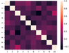 |
Fig. B.1. 10 × 10 JK correlation coefficient matrix, Rℓℓ′, for the κg NVSS–CMB lensing cross-spectrum evaluated in bins of size Δℓ = 30. The value of the off-diagonal cross-correlation coefficients is color-coded according to the vertical bar. |
To make this statement more quantitative and assess the goodness of the Gaussian model, we compare in Fig. B.2 the diagonal elements of the Gaussian covariance matrix of the cross-spectrum (curves with different colors) with the same elements in the JK covariance matrix (black dots). For the Gaussian cases we plot, in the upper panel, different curves corresponding to the different b(z)+N(z) model combinations assumed to estimate the covariance. Their similarity indicates that Gaussian errors are not very sensitive to the N(z) and b(z) choice. The bottom panel quantifies the percentage difference between the Gaussian errors and the JK errors. The differences between the two types of errors oscillate with ℓ with a modest amplitude on the order of 10%. Moreover, the fact that these oscillations are on the same order of those seen in the black curve around its smoothed interpolation suggests that uncertainties in the estimate of the JK errors are on the same order of the differences between JK and Gaussian estimates, that is, the per cent discrepancies in the bottom panel are not solely driven by deviations from the Gaussian hypothesis. We also notice that differences among Gaussian errors obtained with various N(z) and b(z) schemes steadily decrease with ℓ.
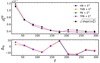 |
Fig. B.2. Gaussian vs. JK errors for the κg NVSS cross-spectrum estimated in bins Δℓ = 30 in the range 11 ≤ ℓ ≤ 310. Upper panel: Gaussian errors for different b(z)+N(z) model combinations, specified in the labels, shown as colored dots and dashed curves. Black dots and dashed curve indicate JK errors. Errors have been estimated from the diagonal elements of the Gaussian covariance (Eq. 18) and JK covariance (Eq. B.1). Bottom panel: Per cent difference between the Gaussian and JK errors. |
In our analysis, we considered binned spectra and we chose a bin size Δℓ = 30. As anticipated, we set the size wide enough to guarantee that the hypothesis of Gaussian statistics would hold and that a Gaussian model could have been adopted to perform the χ2 analysis. To justify this choice, we repeated the analysis using different bin sizes Δℓ = 20, 30 and 50 and compared the results obtained using a Gaussian versus a JK covariance matrix. The idea is that the two sets of results need to be consistent, and a smaller  would be obtained for the bin size Δℓ that minimizes the error covariance while preserving the information.
Since the results are not very sensitive to the choice of N(z) and b(z), in Table B.1 we only show the ones obtained for the combination S3 and TPB. When the Gaussian errors are used (second column), the  value steadily increase with the bin size (and, correspondingly, the PTE decreases). We interpret this result as evidence that, when the number of bins is reduced, the statistical significance of the mismatch at small ℓ values increases. The case with the JK errors (third column) is different. The dependence of
  value on Δℓ is not monotonic. There is a soft spot at Δℓ = 30 in correspondence of which the reduced
  value is similar to the one obtained in the Gaussian case. Moreover, for Δℓ = 20 the reduced
  value of the Gaussian analysis, which ignores error covariance altogether, is smaller than the JK one. This suggests that with this bin size the Gaussian errors could be overestimated. Therefore, we decided to make a conservative choice and adopt, for the analysis presented in this work, Δℓ = 30.
Reduced  values and PTE as a function of bin size, Δℓ.
The adequacy of this choice is corroborated by the results obtained with other N(z) and b(z) models. Adopting, for example, the T-RECS + TPB combination we find reduced  values that are on average 30 % smaller than those obtained with the S3 case. However, the
  behavior is the same, including the existence of a soft spot at Δℓ = 30 for the JK case and the corresponding similarity between the
  values of the Gaussian and JK analyses. We perform a similar test for the TGSS catalog and the behavior of
  as a function of Δℓ is in agreement with the one discussed above for NVSS.
B.2. Simulation-based tests
In this section we provide a further validation of the analytic Gaussian approximation adopted for the power spectrum covariance matrix by performing two different sets of tests based on simulations. As a by-product, the tests also demonstrate that our pipeline is unbiased.
As a first approach, we cross-correlate 300 realistic simulations of the Planck CMB lensing convergence10 (Planck Collaboration VIII 2020) with the radio source maps of both NVSS and TGSS. Each simulation contains a realization of the CMB lensing convergence, drawn from the Planck best-fit power spectrum, plus realistic lensing reconstruction noise, which also properly accounts for the fact that the reconstruction has been performed on a masked sky. When extracting the cross-angular power spectra we employ the same masks used in our main analysis. Then, the covariance matrix is estimated from the simulated cross-spectra. However, lensing simulations and radio source data maps are in principle uncorrelated, unless there are anomalous features in the latter that can produce spurious correlations. As a consequence, this procedure does not account for the cosmic variance contribution to the uncertainties that should come from the correlated part of the maps,  . Regardless, we expect the estimated covariance to be fairly representative as both lensing and galaxy maps are noise dominated at the relevant scales used in our analysis. In Fig. B.3 we show the mean recovered cross-spectrum from simulations and the 1 σ errors obtained as the standard deviation of the simulated spectra. Finding that the mean cross-spectrum is consistent with zero serves as a powerful check that: a) our analysis pipeline does not induce any spurious bias; b) the large-scale anomalous power in TGSS does not correlate with CMB lensing and its reconstruction noise. The figure also provides a comparison to the analytic Gaussian uncertainties used in our main analysis, which are shown with the gray band. We can appreciate a good agreement between the two, with the only exception of the uncertainty in the first bin for TGSS. In this case, the uncertainty from simulations is larger by ∼25%; this is a consequence of the excess power at large scales in the TGSS clustering, which is not reproduced by any theoretical model. Nevertheless, we verified that this difference has negligible impact on the χ2 analysis and does not alter the conclusions of our work. Finally, checking the off-diagonal elements of the covariance matrix estimated from simulations, we verified that bin-to-bin correlations are < 20% everywhere.
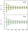 |
Fig. B.3. Mean recovered cross-power spectra from realistic simulations of Planck CMB lensing convergence and NVSS or TGSS data maps (in green). The spectra are consistent with zero, demonstrating that our analysis pipeline does not induce spurious cross-power in the absence of correlation (see text). Error bars are the diagonal elements of the empirical covariance matrix derived from the same simulations. They need to be compared with the gray bands that represent the analytic Gaussian uncertainties used throughout the paper. In the top panel, in orange, we also show the mean cross-power spectrum from Gaussian-correlated lensing and galaxy simulations minus the input theoretical cross-power spectrum. Consistency with zero implies that our pipeline is able to recover in an unbiased way a known input cross-spectrum. Error bars in this case are the diagonal elements of the empirical covariance matrix derived from the correlated simulations. |
In the second approach, starting from the theoretical spectra of the model corresponding to the combination T-RECS + TPB, we simulate 300 maps of both the galaxy density contrast and the CMB lensing convergence as Gaussian-correlated fields, this time, with the expected level of correlation  (see, e.g., the appendix of Giannantonio et al. 2008). We include the contribution of noise as well, which for the lensing, in this case, has been generated as simple Gaussian white noise from the
  power spectrum, while for the galaxy maps consists in Poisson realizations with the shot noise level Ngg. We estimate the cross-spectra of the simulated maps after applying the same masks used in the main analysis. We only consider the NVSS case, as TGSS will provide similar results given the mask for this catalog is very close to that of NVSS. From Fig. B.3, we can see that our pipeline is able to recover the correct cross-correlation spectrum from the simulations. Moreover, error bars estimated from simulations are in good agreement with the analytic Gaussian uncertainties with differences of at most 15%.
All Tables
Best-fit values for the NVSS bias parameter, bg, and for the shot-noise term, Ngg, obtained from the joint κg and gg power spectra analysis.
All Figures
|
Fig. 1. Mollweide projection in Galactic coordinates of the masked areas in the radio samples (purple) and in the Planck CMB lensing convergence map (turquoise). Top panel: NVSS case. Bottom panel: TGSS case. |
| In the text | |
|
Fig. 2. Redshift distribution models, N(z), for the NVSS (top panels) and TGSS catalogs (bottom panels) shown in the range z = [0, 3]. Predictions from the S3 simulator are shown to the left and T-RECS to the right. The thick black histogram in each panel shows the distributions of all sources in the catalog. Histograms with different colors indicate the distribution of each object type identified by the labels. |
| In the text | |
|
Fig. 3. Bias models used in this work as a function of redshift in the range z = [0, 3] for the NVSS (top panel) and TGSS (bottom panel) cases. Curves with different colors and line styles are used for the different combinations of N(z) and galaxy bias models, as indicated in the labels. The values of the free parameter, bg, are listed in Tables 6 and 7 for TGSS and NVSS, respectively. We also consider “truncated” versions of the HB and PB models, in which the value of the bias for each population of sources is kept constant for z ≥ 1.5 (dashed lines). |
| In the text | |
|
Fig. 4. Binned angular power spectra of NVSS (black diamonds) and TGSS (red dots) sources in the range ℓ = [11, 130]. The size of the bins is Δℓ = 10. Error bars are 1σ Gaussian uncertainties from Eq. (18). Power spectra are corrected for both shot noise and multiple component contributions (see text for details). |
| In the text | |
|
Fig. 5. Cross-angular power spectra of the NVSS catalog (black diamonds) and TGSS catalog (red dots) with CMB lensing convergence in the range ℓ = [11, 310] measured in bins Δℓ = 10. Error bars are the 1σ Gaussian uncertainties from Eq. (18). |
| In the text | |
|
Fig. 6. κg cross-spectrum analysis for the TGSS sample. Red dots represent the estimated power spectrum while error bars correspond to 1σ Gaussian uncertainties. Curves with different colors are theoretical predictions of different b(z)+N(z) combinations, as specified by the labels. Top panel: models that use the S3N(z). Bottom panel: models that use the T-RECS N(z) predictions. |
| In the text | |
|
Fig. 7. Same as Fig. 6 but for the NVSS κg cross-spectrum analysis. The estimated power spectrum is shown with black diamonds. Error bars represent 1σ Gaussian uncertainties. |
| In the text | |
|
Fig. 8. Best-fit κg power spectra models for the TGSS sample (solid and dashed lines) vs. measured (red dots) and their 1σ Gaussian error bars. Different colors and line styles are used for the different redshift distribution models: N(z) from T-RECS (green) and N(z) from S3 (purple). Continuous lines refer to a linearly evolving bias (model 1) while dashed lines to a constant bias (model 2). The best fitting bg values are listed in Table 6. |
| In the text | |
|
Fig. 9. Same as Fig. 8 but considering the NVSS sample. Data are now shown with black diamonds along with their 1σ error bars. Colors and line styles of the model cross-spectra are also the same. Values of the best-fit bg are summarized for the different models in Table 7. |
| In the text | |
|
Fig. 10. Marginalized 1D probability distributions, P1D, of bg for different bias models. The continuous curves show P1D for model 1 (constant bias) and model 2 (linearly growing bias), obtained from the joint NVSS gg and κg power spectrum analysis. All curves are normalized so that P1D = 1 at the maximum. Different colors indicate the different N(z) models and match those used in Fig. 9. Dotted curves are drawn for comparison and show the P1D from the NVSS cross-spectrum-only analysis. They are labeled CA to further distinguish them from those obtained from the joint analysis, labeled JA. |
| In the text | |
|
Fig. 11. Model vs. measured NVSS κg (top panels) and gg (bottom panels) angular power spectra. The measured cross-spectra (top panels) are the same as in the previous plots. Error bars represent 1σ Gaussian uncertainties. The curves show model predictions. They are surrounded by shaded areas that represent the 2σ uncertainty interval of the best fitting bg values. The green color in the left panels indicates models that adopt the T-RECS N(z) prescription. The purple color flags the adoption of the S3 model in the right panels. Continuous and dashed lines are used for bias model 1 and model 2, respectively. All best fitting bg values are listed in Table 8. |
| In the text | |
|
Fig. 12. Residuals, |
| In the text | |
|
Fig. 13. Cross-angular power spectra for NVSS (top) and TGSS (bottom) with different Planck CMB lensing reconstructions obtained with temperature-only data (TT), polarization-only data (PP), and their MV combination. To estimate the spectra, we used the baseline mask and a multipole bin size Δℓ = 50. |
| In the text | |
|
Fig. 14. Residuals, |
| In the text | |
|
Fig. 15. Probability distribution functions for the magnification bias parameter, |
| In the text | |
|
Fig. B.1. 10 × 10 JK correlation coefficient matrix, Rℓℓ′, for the κg NVSS–CMB lensing cross-spectrum evaluated in bins of size Δℓ = 30. The value of the off-diagonal cross-correlation coefficients is color-coded according to the vertical bar. |
| In the text | |
|
Fig. B.2. Gaussian vs. JK errors for the κg NVSS cross-spectrum estimated in bins Δℓ = 30 in the range 11 ≤ ℓ ≤ 310. Upper panel: Gaussian errors for different b(z)+N(z) model combinations, specified in the labels, shown as colored dots and dashed curves. Black dots and dashed curve indicate JK errors. Errors have been estimated from the diagonal elements of the Gaussian covariance (Eq. 18) and JK covariance (Eq. B.1). Bottom panel: Per cent difference between the Gaussian and JK errors. |
| In the text | |
|
Fig. B.3. Mean recovered cross-power spectra from realistic simulations of Planck CMB lensing convergence and NVSS or TGSS data maps (in green). The spectra are consistent with zero, demonstrating that our analysis pipeline does not induce spurious cross-power in the absence of correlation (see text). Error bars are the diagonal elements of the empirical covariance matrix derived from the same simulations. They need to be compared with the gray bands that represent the analytic Gaussian uncertainties used throughout the paper. In the top panel, in orange, we also show the mean cross-power spectrum from Gaussian-correlated lensing and galaxy simulations minus the input theoretical cross-power spectrum. Consistency with zero implies that our pipeline is able to recover in an unbiased way a known input cross-spectrum. Error bars in this case are the diagonal elements of the empirical covariance matrix derived from the correlated simulations. |
| In the text | |
Current usage metrics show cumulative count of Article Views (full-text article views including HTML views, PDF and ePub downloads, according to the available data) and Abstracts Views on Vision4Press platform.
Data correspond to usage on the plateform after 2015. The current usage metrics is available 48-96 hours after online publication and is updated daily on week days.
Initial download of the metrics may take a while.