© The Authors 2023

1. Introduction

Several papers have reported excesses of the flux densities of high-redshift galaxies in broad bands. For instance, a boost of the Spitzer/IRAC bands at z ∼ 7–8 is observed when Hα, and [OIII]500.7 nm fall in the mid-infrared (mid-IR) filters (e.g., de Barros et al. 2013; Roberts-Borsani et al. 2020; Anders 2003). In the sub-millimetre (sub-mm) as well, Seaquist et al. (2004) suggested that about 25% of the 850 μm flux density could be due to the CO(3–2) molecular emission. More relevant to this paper, Smail et al. (2011) estimated that a [CII]158 μm fine structure line with 0.27% of the galaxy’s L_dust would contribute 5–10% to the far-IR broadband flux densities at 850 μm. Because the line contribution scales linearly with L_[CII]/L_dust, the [CII]158 μm -to-dust-continuum luminosity ratio and sources with L_[CII]/L_dust > 1% will contribute more than four times this amount, reaching 20–40% of the 850 μm flux densities for galaxies at z ∼ 4–6 (also see Seymour et al. (2012) for the contribution to the Herschel/SPIRE 500 μm band).

On the contrary, L_[CII]/L_dust presents a deficit for galaxies with large IR surface brightnesses or IR luminosities. Luhman et al. (2003) proposed that this deficit could be due to high values of the ionisation parameter¹ (log₁₀U > −2.5), for which a narrower photodissociation region (PDR) would lead to lower [CII]158 μm fluxes. This explanation is also supported by a number of other analyses (e.g., Abel et al. 2009; Díaz-Santos et al. 2013, 2017; Herrera-Camus et al. 2018).

Recent promising papers concerning the James Webb Space Telescope (JWST, e.g., Schaerer et al. 2022; Trump et al. 2022; Taylor et al. 2022) suggest that we are now able to spectroscopically measure the nebular parameters of galaxies in the epoch of reionisation (EoR) at z ∼ 5–8. However, we still have large uncertainties when estimating the obscured star formation density at high redshift (e.g., Algera et al. 2023). Thus, we still need to identify and measure the luminosities of galaxies in the EoR to better understand how the total star formation rate density (SFRD) evolves in the early Universe to understand the formation and early evolution of galaxies at z > 10 (e.g., Finkelstein et al. 2022).

In this paper, we propose an original method to identify 4.5 < z < 6.0 galaxies via a broad-band excess due to the [CII]158 μm line. This method is applicable to very large numbers of dusty galaxies that can be extracted from the already existing far-IR and sub-millimetre databases (Sect. 3). We present tests on a sample of galaxies with spectroscopic redshifts observed with the South Pole Telescope (SPT, Sect. 2) that seem to confirm the validity of the above method (Sect. 4). This method simultaneously provides a way to constrain the nebular parameters of galaxies at 2 < z < 7 (Sect. 5). Moreover, the same method could be utilised for different redshift ranges and different photometric bands.

We assumed a Chabrier initial mass function (IMF, Chabrier 2003). We used WMAP7 cosmology (Komatsu et al. 2011). Finally, we assumed a solar metallicity Z_⊙ = 0.014 from Asplund et al. (2009).

2. The SPT galaxy sample

Reuter et al. (2020) presented the final spectroscopic redshift analysis of a flux-limited (S_870 μm > 25 mJy) sample of galaxies from the 1.4 mm SPT survey. In this 2500-square-degree survey observed at 1.4 mm and 2.0 mm, they identified 81 strongly lensed, dusty star-forming galaxies (DSFGs) at 1.9 ≲ z ≲ 6.9. The spectroscopic observations were conducted with the Atacama Large Millimeter/submillimeter Array (ALMA) across the 3 mm spectral window, targeting carbon monoxide line emission. From them, spectroscopic redshifts have been estimated by combining ALMA data with ancillary data. They are used in the rest of this paper, and we did not estimate them when fitting the observed spectral energy distributions (SED) or when estimating the physical parameters.

With APEX/LABOCA, Strandet et al. (2016) obtained 870 μm flux densities in the period from 2010 September – 2012 November. The Herschel/SPIRE maps at 250 μm, 350 μm, and 500 μm were observed in two observing programmes, in the period from 2012 August – 2013 March. As described in Strandet et al. (2016), the flux densities were extracted by fitting a Gaussian to the source. The peak of the Gaussian is taken as the flux density. The noise was estimated by taking the RMS in the central few arcmins of the map, which was then added in quadrature to the uncertainty due to pixelation. The data themselves are from Reuter et al. (2020).

This SPT galaxy sample contains bright IR galaxies that might include an active galactic nucleus (AGN). So, a preliminary check is needed to see if an AGN can substantially modify the IR spectral energy distribution of galaxies. However, none of the attempted observations were able to confirm the presence of an AGN in these objects, or at least not a strong AGN. De Breuck et al. (2019) derived a low AGN fraction² (frac_AGN < 5%) for SPT 0418-47, and they claim that this is consistent with the AGN fractions estimated in other DSFGs from the SPT sample. In the galaxy SPT 2132-58, Béthermin et al. (2016) identified an evolved interstellar medium (ISM) with 0.5 < Z/Z_⊙ < 1.5, dominated by PDRs. Its CO spectral line energy distribution does not allow us to reach a conclusion on the presence or absence of an AGN. Gururajan et al. (2022) showed that the presence of an AGN in SPT 0103-45 is unlikely (see also, Ma et al. 2016; Spilker et al. 2018). Finally, Apostolovski et al. (2019) found no signs for a signature pointing to the presence of an AGN in SPT 0346-52. Thus, for the sake of the present paper, we made the assumption that there are no major AGNs in the studied sample.

3. A colour-colour approach for the selection of galaxies at z > 4

We modelled the Herschel and APEX/LABOCA colours ${log}_{10}\frac{{\mathrm{PSW}}_{250\mathrm{\mu }\mathrm{m}}}{{\mathrm{PMW}}_{350\mathrm{\mu }\mathrm{m}}}$ and ${log}_{10}\frac{{\mathrm{LABOCA}}_{870\mathrm{\mu }\mathrm{m}}}{{\mathrm{PLW}}_{500\mathrm{\mu }\mathrm{m}}}$ with CIGALE (Burgarella et al. 2005; Noll et al. 2009; Boquien et al. 2019). With the input CIGALE parameters listed in Table 1, CIGALE creates 88 million models. This particular set of colours is selected to try and identify line-boosted galaxies at z ≳ 4–6 as outliers in the above colour-colour diagram.

A grid of nebular emission lines that includes HII regions and PDRs are pre-computed with CLOUDY (Ferland et al. 2017) by varying the nebular parameters N_e, Z_gas, and U. These emission lines are included into CIGALE when building the modelled spectra (Fig. 1). The photo-ionising field shape is generated with the single stellar population (SSP) model library (Bruzual & Charlot 2003) using a constant star formation history (SFH) over 10 Myr and accounting for a range of metallicities, ionisation parameters, and number densities of hydrogen. The radiation field intensity is given by the dimensionless ionisation parameter U ≡ n_γ/n_H, where n_γ is the number density of photons capable of ionising hydrogen, and n_H the number density of hydrogen, which equals the number density of electrons in a fully ionised medium. The limit of the effective HII region is set by an ionisation fraction ≤10⁻³, while the end of the effective PDR is set by the visual attenuation A_V ≤ 10 (Röllig et al. 2007), and as such includes part of the molecular region. The size and abundance distribution of grains, typical for the ISM of our galaxy, is used to account for the extinction in the PDR; it includes both a graphitic and a silicate component with R_V ≡ A_V/E(B − V) = 3.1. The grain density scales with the hydrogen density n_H. The line fluxes are re-scaled with the number of Lyman continuum photons, extracted from the stellar emission of the modelled galaxies. These line models will be detailed in Theulé et al. (in prep.).

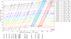Fig. 1. Evolution of CIGALE models with nebular parameters. This sample of models created by CIGALE is an extract of the entire and much larger one used for the SED fitting (88 × 106 models). Here, in addition to the nebular parameters given in the legend, we fix the SFH (delayed with τmain = 500 Myrs, and agemain = 100 Myrs), AV(ISM) = 0.3, Tdust = 40 K, the dust emissivity β = 2.0, and the redshift z = 0. However, to improve the visibility, we offset the spectra by δz = 0.1 on the X axis and 1 dex on the Y axis. The bottom spectra, with log10U = −2 are more representative of the IR spectra emitted by an HII-region dominated galaxy, with a strong [OIII]88.3 μm line (blue-shaded area) detected, for example, in Lyman break galaxies in the early Universe. The top spectra, with log10U = −4, resemble an IR spectra emitted by a PDR-dominated galaxy, with a strong [CII]157.6 μm line (red-shaded area), detected, for example, in DSFGs in the early Universe. A higher gas metallicity amplifies the strength of the metal lines.

For the dust emission, we selected the modified blackbody module in CIGALE, with a power law in the mid-IR (Casey 2012). In Fig. 2, we present the dust temperature and the Rayleigh-Jeans slope (T_dust and β_RL) controlling the shape of the IR continuum SEDs that are derived by fitting the observed SEDs with CIGALE. T_dust and β_RL derived by fitting the data are only meant to check their measured range. They are not used in the rest of the analysis. The CIGALE mock analysis, also presented in Fig. 2, suggests that T_dust and β_RL can be well estimated, with a coefficient of correlation of r² = 0.92 for T_dust and r² = 0.80 for β_RL.

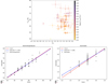Fig. 2. How the dust continuum was taken into account in the analysis. Top panel shows the distribution of Tdust and βRL for the SPT sample. In the bottom panel, we used the CIGALE mock analysis to check whether Tdust and βRL can be correctly estimated using the available set of data for this SPT sample. In this mock analysis, we use the best models and each of the exact parameters used to build the models for each of the objects. We add the observed noise to the models, and refit the simulated data to re-estimate the same dust and βRL parameters. A good correlation between the ‘estimated’ and the ‘exact’ Tdust and βRL suggests that we are able to derive them correctly.

In Fig. 3, the modelled colours are compared to the observed ones in the colour-colour diagram with and without adding emission lines to the modelled continuum. As above, we assume a mid-IR power law and a modified blackbody with a dense sampling in dust temperature, T_dust, and emissivity, β_RL, to best reproduce the rest-frame far-IR dust continuum emission.

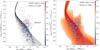Fig. 3. Models computed by CIGALE for the [${log}_{10}\frac{{\mathrm{PSW}}_{250\mathrm{\mu }\mathrm{m}}}{{\mathrm{PMW}}_{350\mathrm{\mu }\mathrm{m}}}$ versus ${log}_{10}\frac{{\mathrm{LABOCA}}_{870\mathrm{\mu }\mathrm{m}}}{{\mathrm{PLW}}_{500\mathrm{\mu }\mathrm{m}}}$] colours. Left: when no fine structure emission lines are added to the modelled spectra, the modelled galaxies are mainly located on a prime sequence extending from the bottom right to the top left. However, a clump of high-redshift observed galaxies, with colours [${log}_{10}\frac{{\mathrm{PSW}}_{250\mathrm{\mu }\mathrm{m}}}{{\mathrm{PMW}}_{350\mathrm{\mu }\mathrm{m}}}$ versus ${log}_{10}\frac{{\mathrm{LABOCA}}_{870\mathrm{\mu }\mathrm{m}}}{{\mathrm{PLW}}_{500\mathrm{\mu }\mathrm{m}}}$] ≈ [−0.1, −0.1], and with a total offset from the main sequence of the order of Δcolour ∼ 0.1 − 0.2 cannot be reached by these models without emission lines. Right: emission lines are added to the continuum. When large equivalent width fine structure lines (and more specifically, EW([CII]157.6 μm) ∼ 10–20 μm) are added (Appendix A), the CIGALE models cover this clump of high-redshift galaxies. The three highest points are only partially covered by the models. Even though the two top ones (namely SPT0243-49 and SPT0245-63) are clearly high-redshift objects, respectively at z = 5.702 and z = 5.626, we assumed that the partial coverage is not sufficient and do not use these two objects in the rest of the paper. For the third one (SPT0348-62 at z = 5.654), the coverage by the models allows us to keep it in the analysis. We also identify SPT0418-47, for which we have five emission lines in the considered wavelength range, and an amplification factor of μ = 32.70 (Reuter et al. 2020).

The main apparent trend observed in the colour-colour diagram without emission lines, is a redshift-related sequence from the bottom right to the top left of the plot. This prime sequence is due to the peak of the IR dust emission, passing in the broad bands (see e.g., Amblard et al. 2010). When no fine structure emission lines are added in CIGALE models, all the models are located in, or just below this prime sequence. However, we can see in Fig. 3 that a clump of objects is located above the prime sequence, at [${log}_{10}\frac{{\mathrm{PSW}}_{250\mathrm{\mu }\mathrm{m}}}{{\mathrm{PMW}}_{350\mathrm{\mu }\mathrm{m}}}$, ${log}_{10}\frac{{\mathrm{LABOCA}}_{870\mathrm{\mu }\mathrm{m}}}{{\mathrm{PLW}}_{500\mathrm{\mu }\mathrm{m}}}$] ≈ [−0.1, −0.1], with a total offset from the main sequence of the order of Δ_colour ∼ 0.10 − 0.20. This clump contains most of the highest redshift galaxies at z ≳ 4–6. They cannot be explained by changes in the dust continuum only. In Appendix A, we quantitatively explore the possibility that emission lines are the most important piece of this puzzle. We find that galaxies exhibiting large [CII]157.6 μm equivalent width (EW) reaching EW([CII]157.6 μm) ∼ 10–20 μm could explain such outliers. This is in agreement with the estimates from Smail et al. (2011), which found that the [CII]158 μm line could provide as much as 40% of the 850 μm broadband flux density for z ∼ 4–6 galaxies, when L_[CII]/L_dust > 1%.

Figure 4 compares the evolution in redshift of a model with emission lines, when the PDR dominates the nebular emission (log₁₀U = −4.0), and that of a model also with emission lines, but when the HII regions dominate the nebular emission (log₁₀U = −2.0). Both are also compared to the same models (i.e. for the same dust temperature, T_dust, and dust emissivity on the Rayleigh-Jeans side, β_RL) without lines. The [CII]157.6 μm has a strong impact on the colours of PDR-dominated models. The models with large EWs ([CII]157.6 μm) entering the LABOCA_870 μm band at z ∼ 4–6 can explain the clump of galaxies above the prime sequence. At lower redshifts and for HII models, the combination of the [OIII]51.7 μm, and [OIII]88.3 μm lines (and others at lower levels) also impacts on the broad band colours, and offsets the models to below the prime sequence on the ${log}_{10}\frac{{\mathrm{LABOCA}}_{870\mathrm{\mu }\mathrm{m}}}{{\mathrm{PLW}}_{500\mathrm{\mu }\mathrm{m}}}$ axis. However, some of the models without lines overlap with this region (Fig. 3), which makes the identification of galaxies in this redshift range less conclusive for galaxies dominated by HII regions.

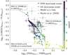Fig. 4. Evolution of the predicted colours with redshift. When compared to models without lines (crosses), at log10U = −4.0 (upward triangles), the strong [CII]157.6 μm line induces an upward move of log10 $\frac{{\mathrm{LABOCA}}_{870\mathrm{\mu }\mathrm{m}}}{{\mathrm{PLW}}_{500\mathrm{\mu }\mathrm{m}}}$ that corresponds to the clump of galaxies at z ∼ 4–6. However, even though the move of the [OIII]51.8 μm and [OIII]88.3 μm lines of galaxies with a strong emission from HII regions at log10U = −2.0 (downward triangles) could induce specific colours, the effect is less clear as models with no lines can also lie in this same region of the plot (Fig. 3). All the symbols are colour-coded by redshift.

4. A colour-colour approach to estimate the nebular parameters of SPT galaxies

We saw the impact of emission lines on the colour distributions. We now try to constrain the physical parameters driving the intensity of the emission lines. For each of the SPT objects, we compute the mean of the models that lie inside ellipses delimited by the uncertainties in both colours. We stress that for each object we only keep the models within δz = ±0.1 from the spectroscopic redshift. This provides us with the mean and standard deviation of the physical parameters used to compute the models, as well as those for the line and continuum fluxes. As already mentioned, the top two objects are very partially covered by the models in Fig. 3: SPT0243-49 and SPT0245-63 at z = 5.702 and z = 5.626, respectively. They are not used hereafter.

We compare the modelled and observed colours in Fig. 5. The regressions provide correlation coefficient of 0.997 for the LABOCA_870 μm/PLW colour and 0.957 for the PSW/PMW colour. The median and standard deviations of the modelled-to-observed colour differences (Δ[log₁₀(Colour_Modelled)−log₁₀(Colour_Observed)] = 0.001 ± 0.036 for the PSW/PMW colour and 0.003 ± 0.011 for the LABOCA_870 μm/PLW colour.

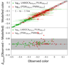Fig. 5. Comparison of compared and observed colours. This figure shows that we can reproduce the observed colours with the CIGALE models. Top: modelled colours (green boxes for ${log}_{10}\frac{{\mathrm{LABOCA}}_{870\mathrm{\mu }\mathrm{m}}}{{\mathrm{PLW}}_{500\mathrm{\mu }\mathrm{m}}}$ and red dots for ${log}_{10}\frac{{\mathrm{PSW}}_{250\mathrm{\mu }\mathrm{m}}}{{\mathrm{PMW}}_{350\mathrm{\mu }\mathrm{m}}}$) are in excellent agreement with the observed ones within the observed uncertainties. The black line shows the one-to-one line, and the grey shaded area presents the boundaries at ±5% (y = 0.95 x and y = 1.05 x). Bottom: This conclusion is confirmed in this panel, where we present the absolute differences in the logarithm of the two colours used in Fig. 3. In both panels, the red circled point corresponds to SPT0348-62, which is already identified in Fig. 3 as one of the objects only partially covered by the models.

In order to check our results, we compare the observed emission line fluxes of the SPT sample to our modelled ones in Fig. 6. However, this comparison is limited because only a small sample of SPT galaxies has been spectroscopically observed, and most of them only with one line.

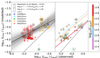Fig. 6. Comparison of the CIGALE-derived line-to-dust luminosities to the observed ones. Left: comparison of observations and models for the spectroscopic sample of SPT galaxies. Most data are from [CII]157.6 μm (Lagache et al. 2018) and [NII]205.2 μm (Cunningham et al. 2020), except for SPT 0418-47 (De Breuck et al. 2019), for which we have several lines. Generally speaking, the brightest [CII]157.6 μm and [OIII]88.3 μm lines are better modelled than the [NII]122. μm and [NII]205.2 μm. The [OI]145. μm is an outlier in this frame. It could be because the former lines are stronger than the latter, or because of physical differences between them. Right: Symbols are colour-coded by intrinsic dust luminosity. The fits suggest that the objects with log10 Ldust < 12.7 and log10 Ldust > 13.5 are found closer to the one-to-one line, or vice versa, meaning that the line predictions for those with 12.7 < log10 Ldust < 13.5 are worse. The objects with a large green circle correspond to the sole object with different lines: SPT0418-47 from De Breuck et al. (2019) (see left panel to identify the lines).

For a sub-sample of the SPT galaxies, Lagache et al. (2018) agreed that [CII]157.6 μm at high redshift mainly originates from the PDR. For the objects in common with the present sample, their [CII]157.6 μm luminosities are compared to our derived [CII]157.6 μm luminosities. Cunningham et al. (2020) showed that 57% of the SPT sample presents an L_{[CII]157.6 μm}/L_{[NII]205.2 μm} luminosity ratio (or lower limit) in agreement with those expected from PDR (or shock regions). However, they suggest that a sub-sample (∼27%) of the 3 < z < 6 SPT galaxies would be consistent (within uncertainties) with a hybrid regime between the model predictions of PDR emission and HII regions. For the objects in common with the present sample, their [NII]205.2 μm luminosities are compared to our derived [NII]205.2 μm luminosities.

Statistical tests are performed with the Python LINMIX library (Fig. 6). This LINMIX method presents the advantage of using a hierarchical Bayesian approach for the linear regression, which takes errors in both X and Y into account (Kelly 2007). The tests are significant (see Fig. 6), given the number of points and the linear correlation coefficient between the observed and modelled fluxes: r = 0.62. We check whether the different locations of the lines, and most notably [CII]158 μm and [NII]205 μm for the present sample, are due to the physical mechanisms producing these two lines. However, we could not pinpoint any differences in the critical densities or ionisation potentials that could explain the differences in the figure (see e.g., Fig. 2 in Spinoglio et al. 2015). We tentatively conclude that the main reason for the increased distance to the one-to-one line is very likely the difference in line intensity for [CII]158 μm and [NII]205 μm. In other words, this method is certainly more sensitive to strong lines (CII and OIII) than to faint lines (NII). The fact that there is about one order of magnitude offset between the observed and modelled line fluxes, for the weak lines, is a limitation for the method presented in this paper because the nebular parameters are based on line ratios. We note, however, another horizontal structure that does not seem random. The redshift does not explain this structure. The galaxies with an intrinsic (i.e. corrected for the amplification using Reuter et al. 2020) dust luminosity (log₁₀L_dust) in the 12.7 < log₁₀ L_dust < 13.5 range are generally found at larger distances, above the one-to-one line. On the contrary, galaxies with log L_dust < 12.7 and galaxies with log log₁₀ L_dust > 13.5 are significantly closer to this one-to-one line. No clear physical origin is identified for this differential effect, though. It could be related to the evolution of these very exotic high redshift objects. More data, and especially rest-frame UV (from JWST) and far-IR (from ALMA or NOEMA) morphologies are fundamental clues to deciphering the structure of this diagram.

From the present SPT sample, only for SPT0418-47 do we have several emission lines (identified with large open circles in the right panel of Fig. 6) that allow us to check how well we model the line ratios. Three of the L_line/L_{[OIII]88.3 μm} modelled ratios are in agreement, within a factor of three at most, to the observed ones (L_[NII]122μm/L_{[OIII]88.3μm} = 0.048 ± 0.014, L_[CII]158μm/L_{[OIII]88.3 μm} = 0.667 ± 0.091, and L_{[NII]205 μm}/L_{[OIII]88.3μm} = 0.032 ± 0.004), while our estimates are 0.143, 0.619, and 0.085, respectively. The observed L_{[OI]145 μm}/L_{[OIII]88.3 μm} = 0.189 ± 0.050, while we find 0.011. This is a factor of almost 17 for [OI]145 μm, which is significantly larger than the other line ratios. However, De Breuck et al. (2019) also had the same problem: their predicted range for this line is 0.02–1.9 × 10¹⁰ L_⊙, while their detection amounts to 2.1 × 10¹⁰ L_⊙ above the maximum predicted value. The conclusion again is that we need to collect more objects with these line ratios to be able to use a statistical approach and clarify the situation. For SPT0418-47, De Breuck et al. (2019) derived a gas metallicity of 0.3 < Z/Z_⊙ < 1.3 and an ionisation parameter of −3.2 < log₁₀U < −2.0. These values are in reasonable agreement (within the uncertainties) with ours: Z/Z_⊙ ∼ 1.47 ± 1.14 and log₁₀U ∼ −3.02 ± 0.80.

We compute the mean of the model parameters inside ellipses delimited by the observational uncertainties. The metallicities are in the 0.5 ≤ Z/Z_⊙ ≤ 2.5 range and the ionisation parameters cover from −4.0 ≤ log₁₀U ≤ −1.5. (Fig. 7). Very high metallicity objects are rare but observed in the local Universe (Gallazzi et al. 2005; Peeples et al. 2008; Maiolino & Mannucci 2019) with metallicities that extend to > 3Z_⊙. Such high values for the ionisation parameter were also measured in the overlap region of the Antennae galaxies by, for example, Snijders et al. (2007), Kewley et al. (2019). Yeh & Matzner (2012) found that radiation pressure confinement sets an upper limit to log₁₀U = −1 in individual regions. However, when observing unresolved starbursts, the mean values are of the order of log₁₀U = −2.3 due to the variety of regions inside a galaxy. As noted earlier in this paper, the two top most objects in Fig. 3 are either very extreme cases among the diversity of galaxies, or the observed colour uncertainties are underestimated. We do not keep them the analysis. However, they probably deserve targeted studies.

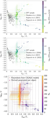Fig. 7. Sequence where we find LBGs at z ∼ 3.3 sample (Onodera et al. 2016) and fit (dashed line) to the sequence from Kojima et al. (2017) are shown in grey. Two different branches are identified for which the [CII]157.6 μm (centre) and [OIII]88.3 μm (top) lines are strong. The top branch contains galaxies that present a [CII] deficit and have a stronger ionisation parameter, log10U ≲ −2.5 while the bottom branch corresponds to galaxies with a normal-to-extreme PDR emission. The bottom panel shows the same information colour-coded with the electronic density, with the grid of models superimposed showing that we should be able to derive metallicities and ionisation parameters in between the two branches.

5. A structure in the log₁₀U versus log₁₀Z/Z_⊙ diagram

From the parameters derived in the previous section, we build the log₁₀U versus Z/Z_⊙ diagram (Fig. 7), where we identify two sequences: the top one with a strong L_{[OIII]88.3 μm} and the bottom one with a strong L_{[CII]157.6 μm} emission. Even though the models are created on a dense regular grid, with a flat probability (bottom panel of Fig. 7), we stress that the metallicities and ionisation parameters derived from the method presented in this paper cannot be precise enough to define the two sequences as clearly as they appear in Fig. 7. The well-defined sequences might be due to the fact that the mean values are estimated from wide probability distribution functions, as confirmed by the uncertainties shown in Fig. 7. The mean values of these wide distributions regularly evolve in the plot, that could suggest the impression of well-defined sequences.

The bottom sequence presents log₁₀U values that are similar to PDR-dominated galaxies, while they are more similar to HII region-dominated galaxies for the top sequence. This type of objects would be galaxies that present a so-called [CII] deficit. These [CII]-deficit galaxies show a ratio of L_{[OIII]88.3 μm}/L_{[CII]157.6 μm} ≈ 3–20 that is about ten times higher than z ∼ 0 galaxies. Harikane et al. (2020) identified nine z = 6–9 galaxies whose observed properties are in agreement with being such [CII] deficit galaxies. Numerous explanations have been proposed: differences in C and O abundance ratios, observational biases, and differences in ISM properties. Carniani et al. (2020) suggested that a surface brightness dimming of the extended [CII] emission would be responsible for the [CII] deficit. Harikane et al. (2020) explained these high L_{[OIII]88.3 μm}/L_{[CII]157.6 μm} ratios by high ionisation parameters or low PDR covering fractions, both of which are consistent with their [NII] observations. This scenario could be reproduced by a density-bound nebula with a PDR deficit. In radiation-hydrodynamics simulations, Abel et al. (2009) concluded that the effects of high ratios of impinging ionising radiation density to particle density (i.e. again, high ionisation parameters) can reproduce the observational characteristics of ultra luminous IR galaxies (ULIRG). When U increases, the fraction of UV photons absorbed by dust increases, and fewer photons are available to photoionise and heat the gas. This leads to a dust-bound nebula, which can explain the observed [CII] deficit (see also Fischer et al. 2014, for a slightly more complex but consistent explanation).

6. Conclusions

We performed an analysis of the SEDs of SPT galaxies with spectroscopic redshifts. We built more than 88 × 10⁶ models with CIGALE and compared the observed objects to the models in a [log₁₀ (PSW_250 μm/PMW_350 μm) versus log₁₀(LABOCA_870 μm/PLW_500 μm)] colour-colour diagram. This set of colours was selected to identify galaxies at z ≳ 4–6 from the influence of the [CII]158 μm fine structure lines on broad bands. This method also allows us to roughly estimate the nebular parameters for this SPT sample.

From this analysis, we find the following results.

• The position of the SPT z ∼ 4–6 galaxies in the colour-colour diagram can only be explained when adding the contribution of fine structure far-IR emission lines to the dust continuum.

• By averaging the models and their associated physical parameters in ellipses delimited by the observed uncertainties in both colours, we can estimate the flux of the fine structure far-IR emission lines, the gas metallicity (Z_gas), and the ionisation parameter (log₁₀U). We find that all the SPT galaxies have a high gas metallicity of 0.6 < Z_gas < 2.5 and they cover a wide range of ionisation parameters in the log₁₀U = −4.0 to -1.5 range. However, we add a word of caution because the faintest lines are overestimated. Thus, line ratios involving faint lines could bias the estimation of nebular parameters.

• In the log₁₀U versus Z_gas diagram, we identify two branches with high [OIII]88 μm/[CII]158 μm ratios for the top branch and low [OIII]88 μm/[CII]158 μm ratios for the bottom branch. The top branch, with high log₁₀U ≲ −2.5, presents a deficit in L_CII/L_dust with respect to the bulk of the galaxy sample, while the bottom branch is the extension of a sequence that continues to LBGs at lower metallicities.

• Without emission lines, outliers are offset from the prime sequence by ∣Δ(log₁₀(PSW_250 μm/PMW_350 μm)∣ ≈ 0.05 and ∣Δ(log₁₀(LABOCA_870 μm/PLW_500 μm)∣ ≈ 0.09. That is a total offset of the order of Δ_total ∼ 0.10. For SPT galaxies at z ≳ 4–6, the main effect is due to [CII]158 μm with 0.6 ≲ EW([CII]157.6 μm) ≲ 25.0 μm. For the most extreme cases, this line could be at the origin of almost half of the flux density at 850 μm, for galaxies at z ∼ 4–6.

• In order to make the most efficient use of this method, a set of medium and broad bands in the mid- and far-IR would be ideal because the effect of the lines would be stronger in narrower bands. One of the caveats of this method is the need to collect an SED as complete as possible to correctly estimate the line fluxes: the more complete the SED, the better the line fluxes can be estimated. Thus, to be efficient, the utility of the method presented here relies on large photometric samples, which are cheaper to obtain than spectroscopy. In other words, our method would benefit from large photometric surveys on a large galaxy sample. Otherwise, spectroscopic observations present the advantage of providing much better estimates. With this configuration, a project like the PRobe far-Infrared Mission for Astrophysics (PRIMA³) allows a statistical approach that would permit us to understand the cosmic rise of metals up to the reionisation. The results found in this paper will be useful for two reasons: the first one is the easier identification of high-redshift galaxies by making use of well-thought colours (as a function of the redshift) in where strong emission lines will produce a measurable excess. The second one by providing a rough but statistical information on nebular parameters for large photometric samples.

Acknowledgments

The authors thank Charles M. (Matt) Bradford for a very useful discussion. DB acknowledges support from the Centre National d’Etudes Spatiales (CNES) for this effort of simulating galaxies and their properties derived from space facilities like Herschel and predict new space observations. Médéric Boquien gratefully acknowledges support by the ANID BASAL project FB210003 and from the FONDECYT regular grant 1211000. A.K.I., Y.S., and Y.F. are supported by NAOJ ALMA Scientific Research grant No. 2020-16B.

References

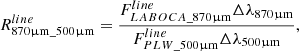
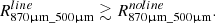
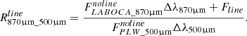
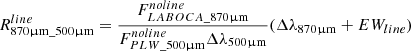
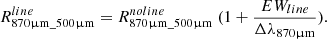
Appendix A: Contribution of emission lines to broad bands

In this appendix, we quantitatively estimate the contribution of the far-IR emission lines to the broad bands. We also show that only the emission lines with the largest equivalent widths, namely [OIII]88.3 μm and [CII]157.6 μm for the considered broad bands and redshift range, could have an impact on the observed colours.

The offset in the colour-colour diagram (Fig. 3) could be due to changes of the PSW_250μm / PMW_350μm and/or the LABOCA_870μm / PLW_500μm colours. Even though this is an over simplification (Fig. A.1), for the sake of clarity, we assume that the main effect is due to [CII]157.6 μm entering or exiting the LABOCA_870μm, and nothing else is modified. The flux density in band PLW_500μm does not change over the redshift range 4 ≲ z ≲ 6. In this case, we have

$$\begin{array}{c}\hfill F_{PLW\_500\mathrm{\mu }\mathrm{m}}^{\mathit{line}}=F_{PLW\_500\mathrm{\mu }\mathrm{m}}^{\mathit{noline}}\&F_{LABOCA\_870\mathrm{\mu }\mathrm{m}}^{\mathit{line}}\gtrsim F_{PLW\_500\mathrm{\mu }\mathrm{m}}^{\mathit{noline}}.\end{array}$$(A.1)

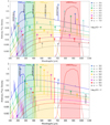Fig. A.1. This figure identifies the emission lines that produce excesses in the broad-bands when the redshift increases. Top: At log10 U = -4.0, the strong [CII]157.6 μm lines enter the LABOCA870μm filters at z ∼ 4 and exit at z ∼ 5.2. The line induces an upward move of the corresponding ${log}_{10}\frac{LABOC{A}_{870\mathrm{\mu }\mathrm{m}}}{PL{W}_{500\mathrm{\mu }\mathrm{m}}}$ colour. [SIII]34.8 μm enters the PSW250μm at z ∼ = 5.5, which boosts the ${log}_{10}\frac{PS{W}_{250\mathrm{\mu }\mathrm{m}}}{PM{W}_{350\mathrm{\mu }\mathrm{m}}}$ colour. We find a total move of the galaxies by about Δtotal ∼ 0.10 in the colour-colour diagram. These two combined effects explain that PDR-dominated galaxies at 4 ≲ z ≲ 6 are offset from the other galaxies. Bottom: Movement of the [OIII]51.8 μm and [OIII]88.3 μm lines of galaxies with a strong emission from HII regions at log10 U = -2.0 could induce specific colours that could help identify such galaxies from this colour-colour diagram. However, the effect is less clear as models with no lines can also lie here (Fig. 3).

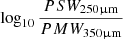
We define the band ratio as follows:

$$\begin{array}{c}\hfill R_{870\mathrm{\mu }\mathrm{m}\_500\mathrm{\mu }\mathrm{m}}^{\mathit{line}}=\frac{F_{LABOCA\_870\mathrm{\mu }\mathrm{m}}^{\mathit{line}}\mathrm{\Delta }{\lambda }_{870\mathrm{\mu }\mathrm{m}}}{F_{PLW\_500\mathrm{\mu }\mathrm{m}}^{\mathit{line}}\mathrm{\Delta }{\lambda }_{500\mathrm{\mu }\mathrm{m}}},\end{array}$$(A.2)

where Δλ_500μm = 143 μm, Δλ_500μm = 186 μm, Δλ_250μm = 67 μm, and Δλ_350μm = 95 μm (SVO Filter Service). Using the right end of Eq. C.1, we have

$$\begin{array}{c}\hfill R_{870\mathrm{\mu }\mathrm{m}\_500\mathrm{\mu }\mathrm{m}}^{\mathit{line}}\gtrsim R_{870\mathrm{\mu }\mathrm{m}\_500\mathrm{\mu }\mathrm{m}}^{\mathit{noline}}.\end{array}$$(A.3)

From Eq. C.2, where F_line is the line flux contributing to the LABOCA_870μm band,

$$\begin{array}{c}\hfill R_{870\mathrm{\mu }\mathrm{m}\_500\mathrm{\mu }\mathrm{m}}^{\mathit{line}}=\frac{F_{LABOCA\_870\mathrm{\mu }\mathrm{m}}^{\mathit{noline}}\mathrm{\Delta }{\lambda }_{870\mathrm{\mu }\mathrm{m}}+F_{\mathit{line}}}{F_{PLW\_500\mathrm{\mu }\mathrm{m}}^{\mathit{noline}}\mathrm{\Delta }{\lambda }_{500\mathrm{\mu }\mathrm{m}}}.\end{array}$$(A.4)

From the left end of Eq. C.1, and the definition of the equivalent width (EW_line), we have 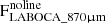${\text{F}}_{\text{LABOCA}\_\text{870}\mathrm{\mu }\text{m}}^{\text{noline}}$ EW_line. This gives:

$$\begin{array}{c}\hfill R_{870\mathrm{\mu }\mathrm{m}\_500\mathrm{\mu }\mathrm{m}}^{\mathit{line}}=\frac{F_{LABOCA\_870\mathrm{\mu }\mathrm{m}}^{\mathit{noline}}}{F_{PLW\_500\mathrm{\mu }\mathrm{m}}^{\mathit{noline}}\mathrm{\Delta }{\lambda }_{500\mathrm{\mu }\mathrm{m}}}(\mathrm{\Delta }{\lambda }_{870\mathrm{\mu }\mathrm{m}}+E{W}_{\mathit{line}})\end{array}$$(A.5)

and, finally,

$$\begin{array}{c}\hfill R_{870\mathrm{\mu }\mathrm{m}\_500\mathrm{\mu }\mathrm{m}}^{\mathit{line}}=R_{870\mathrm{\mu }\mathrm{m}\_500\mathrm{\mu }\mathrm{m}}^{\mathit{noline}}(1+\frac{E{W}_{\mathit{line}}}{\mathrm{\Delta }{\lambda }_{870\mathrm{\mu }\mathrm{m}}}).\end{array}$$(A.6)

The mean colours of the outliers are ⟨log₁₀ (PSW_250μm / PMW_350μm)⟩ = -0.205 ± 0.113 and ⟨log₁₀(LABOCA_870μm / PLW_500μm⟩ = -0.187 ± 0.113. For the same redshift range, CIGALE models without lines give ⟨log₁₀ (PSW_250μm / PMW_350μm)⟩ = -0.254 ± 0.134 and ⟨log₁₀(LABOCA_870μm / PLW_500μm⟩ = -0.101 ± 0.194. The average move needed to reach these galaxies amounts to ∣Δ(log₁₀(PSW_250μm/PMW_350μm)∣ ≈ 0.05 and ∣Δ(log₁₀(LABOCA_870μm/PLW_500μm)∣ ≈ 0.09. That is a total offset of the order of Δ_total ∼ 0.10. Because we cannot know where the galaxy would be without accounting for the emission lines, both colours could contribute to this offset, but it is likely that [CII]157.6 μm is dominant.

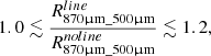
We find that the models inside the ellipses, accounting for the observed uncertainties, have 0.6 ≲ EW([CII]157.6 μm) ≲ 25.0 μm. From this, we obtain

$$\begin{array}{c}\hfill 1.0\lesssim \frac{R_{870\mathrm{\mu }\mathrm{m}\_500\mathrm{\mu }\mathrm{m}}^{\mathit{line}}}{R_{870\mathrm{\mu }\mathrm{m}\_500\mathrm{\mu }\mathrm{m}}^{\mathit{noline}}}\lesssim 1.2,\end{array}$$(A.7)

$$\begin{array}{c}\hfill 0.0\lesssim \mathrm{\Delta }({log}_{10}(LABOC{A}_{870\mathrm{\mu }\mathrm{m}}/PL{W}_{500\mathrm{\mu }\mathrm{m}})\lesssim 0.1,\end{array}$$(A.8)

which is an offset in the colour-colour diagram of ≲ 0.1, that is, about the same order or the maximum one observed.

The [SIII]33.47 μm line enters the PSW_250μm at about the same redshift range and modifies log₁₀ (PSW_250μm / PMW_350μm). However, with 0.05 ≲ EW([SIII]33.5 μm) ≲ 0.26, we estimate that the [SiII]33.47 μm line should not significantly contribute to the PSW_250μm band.

No CIGALE models at δz = ±0.5 match the two highest objects in Fig. 3 (SPT0245-63 at z = 5.626 and SPT0243-49 at z = 5.702), and we cannot estimate any of the physical parameters. The reasons why we cannot reproduce the colours of these two objects is uncertain. Two plausible hypotheses could be made, though. First, the flux densities of these objects might not be correct, or, at least, the uncertainties could be underestimated. The other explanation might be that our present grid of models might not cover the entire possible range of data. These two objects deserve a closer analysis.

All Tables

All Figures

Fig. 1. Evolution of CIGALE models with nebular parameters. This sample of models created by CIGALE is an extract of the entire and much larger one used for the SED fitting (88 × 106 models). Here, in addition to the nebular parameters given in the legend, we fix the SFH (delayed with τmain = 500 Myrs, and agemain = 100 Myrs), AV(ISM) = 0.3, Tdust = 40 K, the dust emissivity β = 2.0, and the redshift z = 0. However, to improve the visibility, we offset the spectra by δz = 0.1 on the X axis and 1 dex on the Y axis. The bottom spectra, with log10U = −2 are more representative of the IR spectra emitted by an HII-region dominated galaxy, with a strong [OIII]88.3 μm line (blue-shaded area) detected, for example, in Lyman break galaxies in the early Universe. The top spectra, with log10U = −4, resemble an IR spectra emitted by a PDR-dominated galaxy, with a strong [CII]157.6 μm line (red-shaded area), detected, for example, in DSFGs in the early Universe. A higher gas metallicity amplifies the strength of the metal lines.

In the text

Fig. 2. How the dust continuum was taken into account in the analysis. Top panel shows the distribution of Tdust and βRL for the SPT sample. In the bottom panel, we used the CIGALE mock analysis to check whether Tdust and βRL can be correctly estimated using the available set of data for this SPT sample. In this mock analysis, we use the best models and each of the exact parameters used to build the models for each of the objects. We add the observed noise to the models, and refit the simulated data to re-estimate the same dust and βRL parameters. A good correlation between the ‘estimated’ and the ‘exact’ Tdust and βRL suggests that we are able to derive them correctly.

In the text

Fig. 3. Models computed by CIGALE for the [${log}_{10}\frac{{\mathrm{PSW}}_{250\mathrm{\mu }\mathrm{m}}}{{\mathrm{PMW}}_{350\mathrm{\mu }\mathrm{m}}}$ versus ${log}_{10}\frac{{\mathrm{LABOCA}}_{870\mathrm{\mu }\mathrm{m}}}{{\mathrm{PLW}}_{500\mathrm{\mu }\mathrm{m}}}$] colours. Left: when no fine structure emission lines are added to the modelled spectra, the modelled galaxies are mainly located on a prime sequence extending from the bottom right to the top left. However, a clump of high-redshift observed galaxies, with colours [${log}_{10}\frac{{\mathrm{PSW}}_{250\mathrm{\mu }\mathrm{m}}}{{\mathrm{PMW}}_{350\mathrm{\mu }\mathrm{m}}}$ versus ${log}_{10}\frac{{\mathrm{LABOCA}}_{870\mathrm{\mu }\mathrm{m}}}{{\mathrm{PLW}}_{500\mathrm{\mu }\mathrm{m}}}$] ≈ [−0.1, −0.1], and with a total offset from the main sequence of the order of Δcolour ∼ 0.1 − 0.2 cannot be reached by these models without emission lines. Right: emission lines are added to the continuum. When large equivalent width fine structure lines (and more specifically, EW([CII]157.6 μm) ∼ 10–20 μm) are added (Appendix A), the CIGALE models cover this clump of high-redshift galaxies. The three highest points are only partially covered by the models. Even though the two top ones (namely SPT0243-49 and SPT0245-63) are clearly high-redshift objects, respectively at z = 5.702 and z = 5.626, we assumed that the partial coverage is not sufficient and do not use these two objects in the rest of the paper. For the third one (SPT0348-62 at z = 5.654), the coverage by the models allows us to keep it in the analysis. We also identify SPT0418-47, for which we have five emission lines in the considered wavelength range, and an amplification factor of μ = 32.70 (Reuter et al. 2020).

In the text

Fig. 4. Evolution of the predicted colours with redshift. When compared to models without lines (crosses), at log10U = −4.0 (upward triangles), the strong [CII]157.6 μm line induces an upward move of log10 $\frac{{\mathrm{LABOCA}}_{870\mathrm{\mu }\mathrm{m}}}{{\mathrm{PLW}}_{500\mathrm{\mu }\mathrm{m}}}$ that corresponds to the clump of galaxies at z ∼ 4–6. However, even though the move of the [OIII]51.8 μm and [OIII]88.3 μm lines of galaxies with a strong emission from HII regions at log10U = −2.0 (downward triangles) could induce specific colours, the effect is less clear as models with no lines can also lie in this same region of the plot (Fig. 3). All the symbols are colour-coded by redshift.

In the text

Fig. 5. Comparison of compared and observed colours. This figure shows that we can reproduce the observed colours with the CIGALE models. Top: modelled colours (green boxes for ${log}_{10}\frac{{\mathrm{LABOCA}}_{870\mathrm{\mu }\mathrm{m}}}{{\mathrm{PLW}}_{500\mathrm{\mu }\mathrm{m}}}$ and red dots for ${log}_{10}\frac{{\mathrm{PSW}}_{250\mathrm{\mu }\mathrm{m}}}{{\mathrm{PMW}}_{350\mathrm{\mu }\mathrm{m}}}$) are in excellent agreement with the observed ones within the observed uncertainties. The black line shows the one-to-one line, and the grey shaded area presents the boundaries at ±5% (y = 0.95 x and y = 1.05 x). Bottom: This conclusion is confirmed in this panel, where we present the absolute differences in the logarithm of the two colours used in Fig. 3. In both panels, the red circled point corresponds to SPT0348-62, which is already identified in Fig. 3 as one of the objects only partially covered by the models.

In the text

Fig. 6. Comparison of the CIGALE-derived line-to-dust luminosities to the observed ones. Left: comparison of observations and models for the spectroscopic sample of SPT galaxies. Most data are from [CII]157.6 μm (Lagache et al. 2018) and [NII]205.2 μm (Cunningham et al. 2020), except for SPT 0418-47 (De Breuck et al. 2019), for which we have several lines. Generally speaking, the brightest [CII]157.6 μm and [OIII]88.3 μm lines are better modelled than the [NII]122. μm and [NII]205.2 μm. The [OI]145. μm is an outlier in this frame. It could be because the former lines are stronger than the latter, or because of physical differences between them. Right: Symbols are colour-coded by intrinsic dust luminosity. The fits suggest that the objects with log10 Ldust < 12.7 and log10 Ldust > 13.5 are found closer to the one-to-one line, or vice versa, meaning that the line predictions for those with 12.7 < log10 Ldust < 13.5 are worse. The objects with a large green circle correspond to the sole object with different lines: SPT0418-47 from De Breuck et al. (2019) (see left panel to identify the lines).

In the text

Fig. 7. Sequence where we find LBGs at z ∼ 3.3 sample (Onodera et al. 2016) and fit (dashed line) to the sequence from Kojima et al. (2017) are shown in grey. Two different branches are identified for which the [CII]157.6 μm (centre) and [OIII]88.3 μm (top) lines are strong. The top branch contains galaxies that present a [CII] deficit and have a stronger ionisation parameter, log10U ≲ −2.5 while the bottom branch corresponds to galaxies with a normal-to-extreme PDR emission. The bottom panel shows the same information colour-coded with the electronic density, with the grid of models superimposed showing that we should be able to derive metallicities and ionisation parameters in between the two branches.

In the text

Fig. A.1. This figure identifies the emission lines that produce excesses in the broad-bands when the redshift increases. Top: At log10 U = -4.0, the strong [CII]157.6 μm lines enter the LABOCA870μm filters at z ∼ 4 and exit at z ∼ 5.2. The line induces an upward move of the corresponding ${log}_{10}\frac{LABOC{A}_{870\mathrm{\mu }\mathrm{m}}}{PL{W}_{500\mathrm{\mu }\mathrm{m}}}$ colour. [SIII]34.8 μm enters the PSW250μm at z ∼ = 5.5, which boosts the ${log}_{10}\frac{PS{W}_{250\mathrm{\mu }\mathrm{m}}}{PM{W}_{350\mathrm{\mu }\mathrm{m}}}$ colour. We find a total move of the galaxies by about Δtotal ∼ 0.10 in the colour-colour diagram. These two combined effects explain that PDR-dominated galaxies at 4 ≲ z ≲ 6 are offset from the other galaxies. Bottom: Movement of the [OIII]51.8 μm and [OIII]88.3 μm lines of galaxies with a strong emission from HII regions at log10 U = -2.0 could induce specific colours that could help identify such galaxies from this colour-colour diagram. However, the effect is less clear as models with no lines can also lie here (Fig. 3).

In the text

References

- Abel, N. P., Dudley, C., Fischer, J., Satyapal, S., & van Hoof, P. A. M. 2009, ApJ, 701, 1147 [Google Scholar]
- Algera, H. S. B., Inami, H., Oesch, P. A., et al. 2023, MNRAS, 518, 6142 [Google Scholar]
- Amblard, A., Cooray, A., Serra, P., et al. 2010, A&A, 518, L9 [NASA ADS] [CrossRef] [EDP Sciences] [Google Scholar]
- Anders, P., & Fritze-v Alvensleben, U., 2003, A&A, 401, 1063 [NASA ADS] [CrossRef] [EDP Sciences] [Google Scholar]
- Apostolovski, Y., Aravena, M., Anguita, T., et al. 2019, A&A, 628, A23 [NASA ADS] [CrossRef] [EDP Sciences] [Google Scholar]
- Asplund, M., Grevesse, N., Sauval, A. J., & Scott, P. 2009, ARA&A, 47, 481 [NASA ADS] [CrossRef] [Google Scholar]
- Béthermin, M., De Breuck, C., Gullberg, B., et al. 2016, A&A, 586, L7 [NASA ADS] [CrossRef] [EDP Sciences] [Google Scholar]
- Boquien, M., Burgarella, D., Roehlly, Y., et al. 2019, A&A, 622, A103 [NASA ADS] [CrossRef] [EDP Sciences] [Google Scholar]
- Bruzual, G., & Charlot, S. 2003, MNRAS, 344, 1000 [NASA ADS] [CrossRef] [Google Scholar]
- Burgarella, D., Buat, V., & Iglesias-Páramo, J. 2005, MNRAS, 360, 1413 [NASA ADS] [CrossRef] [Google Scholar]
- Carniani, S., Ferrara, A., Maiolino, R., et al. 2020, MNRAS, 499, 5136 [NASA ADS] [CrossRef] [Google Scholar]
- Casey, C. M. 2012, MNRAS, 425, 3094 [Google Scholar]
- Chabrier, G. 2003, PASP, 115, 763 [Google Scholar]
- Charlot, S., & Fall, S. M. 2000, ApJ, 539, 718 [Google Scholar]
- Cunningham, D. J. M., Chapman, S. C., Aravena, M., et al. 2020, MNRAS, 494, 4090 [NASA ADS] [CrossRef] [Google Scholar]
- de Barros, S., Nayyeri, H., Reddy, N., & Mobasher, B. 2013, in SF2A-2013: Proceedings of the Annual meeting of the French Society of Astronomy and Astrophysics, eds. L. Cambresy, F. Martins, E. Nuss, & A. Palacios, 531 [Google Scholar]
- De Breuck, C., Weiß, A., Béthermin, M., et al. 2019, A&A, 631, A167 [NASA ADS] [CrossRef] [EDP Sciences] [Google Scholar]
- Díaz-Santos, T., Armus, L., Charmandaris, V., et al. 2013, ApJ, 774, 68 [Google Scholar]
- Díaz-Santos, T., Armus, L., Charmandaris, V., et al. 2017, ApJ, 846, 32 [Google Scholar]
- Ferland, G. J., Chatzikos, M., Guzmán, F., et al. 2017, Rev. Mex. A&A, 53, 385 [Google Scholar]
- Finkelstein, S. L., Bagley, M. B., Arrabal Haro, P., et al. 2022, ApJ, 940, L55 [NASA ADS] [CrossRef] [Google Scholar]
- Fischer, J., Abel, N. P., González-Alfonso, E., et al. 2014, ApJ, 795, 117 [NASA ADS] [CrossRef] [Google Scholar]
- Gallazzi, A., Charlot, S., Brinchmann, J., White, S. D. M., & Tremonti, C. A. 2005, MNRAS, 362, 41 [Google Scholar]
- Gururajan, G., Béthermin, M., Theulé, P., et al. 2022, A&A, 663, A22 [NASA ADS] [CrossRef] [EDP Sciences] [Google Scholar]
- Harikane, Y., Ouchi, M., Inoue, A. K., et al. 2020, ApJ, 896, 93 [Google Scholar]
- Herrera-Camus, R., Sturm, E., Graciá-Carpio, J., et al. 2018, ApJ, 861, 95 [Google Scholar]
- Kelly, B. C. 2007, ApJ, 665, 1489 [Google Scholar]
- Kewley, L. J., Nicholls, D. C., & Sutherland, R. S. 2019, ARA&A, 57, 511 [Google Scholar]
- Kojima, T., Ouchi, M., Nakajima, K., et al. 2017, PASJ, 69, 44 [NASA ADS] [CrossRef] [Google Scholar]
- Komatsu, E., Smith, K. M., Dunkley, J., et al. 2011, ApJS, 192, 18 [Google Scholar]
- Lagache, G., Cousin, M., & Chatzikos, M. 2018, A&A, 609, A130 [NASA ADS] [CrossRef] [EDP Sciences] [Google Scholar]
- Luhman, M. L., Satyapal, S., Fischer, J., et al. 2003, ApJ, 594, 758 [Google Scholar]
- Ma, J., Gonzalez, A. H., Vieira, J. D., et al. 2016, ApJ, 832, 114 [CrossRef] [Google Scholar]
- Maiolino, R., & Mannucci, F. 2019, A&A Rev., 27, 3 [NASA ADS] [CrossRef] [Google Scholar]
- Noll, S., Burgarella, D., Giovannoli, E., et al. 2009, A&A, 507, 1793 [NASA ADS] [CrossRef] [EDP Sciences] [Google Scholar]
- Onodera, M., Carollo, C. M., Lilly, S., et al. 2016, ApJ, 822, 42 [NASA ADS] [CrossRef] [Google Scholar]
- Peeples, M. S., Pogge, R. W., & Stanek, K. Z. 2008, ApJ, 685, 904 [NASA ADS] [CrossRef] [Google Scholar]
- Reuter, C., Vieira, J. D., Spilker, J. S., et al. 2020, ApJ, 902, 78 [NASA ADS] [CrossRef] [Google Scholar]
- Roberts-Borsani, G. W., Ellis, R. S., & Laporte, N. 2020, MNRAS, 497, 3440 [NASA ADS] [CrossRef] [Google Scholar]
- Röllig, M., Abel, N. P., Bell, T., et al. 2007, A&A, 467, 187 [Google Scholar]
- Schaerer, D., Marques-Chaves, R., Barrufet, L., et al. 2022, A&A, 665, L4 [NASA ADS] [CrossRef] [EDP Sciences] [Google Scholar]
- Seaquist, E., Yao, L., Dunne, L., & Cameron, H. 2004, MNRAS, 349, 1428 [CrossRef] [Google Scholar]
- Seymour, N., Altieri, B., De Breuck, C., et al. 2012, ApJ, 755, 146 [NASA ADS] [CrossRef] [Google Scholar]
- Smail, I., Swinbank, A. M., Ivison, R. J., & Ibar, E. 2011, MNRAS, 414, L95 [NASA ADS] [CrossRef] [Google Scholar]
- Snijders, L., Kewley, L. J., & van der Werf, P. P. 2007, ApJ, 669, 269 [NASA ADS] [CrossRef] [Google Scholar]
- Spilker, J. S., Aravena, M., Béthermin, M., et al. 2018, Science, 361, 1016 [NASA ADS] [CrossRef] [Google Scholar]
- Spinoglio, L., Pereira-Santaella, M., Dasyra, K. M., et al. 2015, ApJ, 799, 21 [NASA ADS] [CrossRef] [Google Scholar]
- Strandet, M. L., Weiss, A., Vieira, J. D., et al. 2016, ApJ, 822, 80 [NASA ADS] [CrossRef] [Google Scholar]
- Taylor, A. J., Barger, A. J., & Cowie, L. L. 2022, ApJ, 939, L3 [NASA ADS] [CrossRef] [Google Scholar]
- Trump, J. R., Arrabal Haro, P., Simons, R. C., et al. 2022, AAS J., submitted, [arXiv:2207.12388] [Google Scholar]
- Yeh, S. C. C., & Matzner, C. D. 2012, ApJ, 757, 108 [NASA ADS] [CrossRef] [Google Scholar]