| Issue |
A&A
Volume 682, February 2024
|
|
|---|---|---|
| Article Number | A119 | |
| Number of page(s) | 17 | |
| Section | Extragalactic astronomy | |
| DOI | https://doi.org/10.1051/0004-6361/202347166 | |
| Published online | 12 February 2024 | |
Modeling the spectral energy distribution of starburst galaxies
The role of photodissociation regions
1
Aix-Marseille Univ., CNRS, CNES, LAM, Marseille, France
e-mail: This email address is being protected from spambots. You need JavaScript enabled to view it.
2
Centro de Astronomía (CITEVA), Universidad de Antofagasta, Avenida Angamos 601, Antofagasta, Chile
Received:
12
June
2023
Accepted:
30
November
2023
Abstract
Context. Analyzing multiwavelength observations of galaxies from the far-ultraviolet to the millimeter domains provides a wealth of information on the physical properties of galaxies and their evolution across cosmic time. Existing or upcoming ground-based or space-borne facilities with enhanced sensitivities and resolutions open an unprecedented window on the galaxy evolution in the early Universe. However, the derivation of galaxy properties from nebular emission lines is not trivial because the interstellar medium in a galaxy may be patchy, and emission might originate both from starburst emission regions and from partially covered photon-dominated regions.
Aims. We model both the nebular continuum emission and the line emission of the spectral energy distribution for galaxies exhibiting both a HII region-like emission and emission like that from a photon-dominated regions to account for the partial shielding of the starburst emission region by dense clouds.
Methods. Nebular galactic emission was modeled from far-ultraviolet to millimeter ranges in a two-sector model with an HII region and a photon-dominated region. The partial overlap of the HII region by the photon-dominated region was accounted for by a covering factor. We generated grids of emission spectra using the Cloudy photoionization code for our two-sector model.
Results. We compared our models with spectral lines from different samples of galaxies for which we mixed characteristic emission from starburst regions and denser regions. We show that the infrared line ratios can constrain the density, metallicity, photoionization parameter, and the covering factor. We also built infrared diagnostic diagrams based on different infrared line ratios in which the galaxy location contains information about its physical conditions.
Conclusions. The two-sector model that couples starburst emission regions and photon-dominated regions can span the existing observations. We implement the resulting emission line libraries in the CIGALE galaxy spectral energy distribution code to help interpret spectrophotometric observations.
Key words: methods: data analysis / ISM: lines and bands / photon-dominated region (PDR) / galaxies: evolution / galaxies: high-redshift / galaxies: ISM
© The Authors 2024
 Open Access article, published by EDP Sciences, under the terms of the Creative Commons Attribution License (https://creativecommons.org/licenses/by/4.0), which permits unrestricted use, distribution, and reproduction in any medium, provided the original work is properly cited.
This article is published in open access under the Subscribe to Open model. This email address is being protected from spambots. You need JavaScript enabled to view it. to support open access publication.
1. Introduction
Emission lines are an essential part of the galaxy spectral energy distribution (SED), and observations of these lines by existing or upcoming ground-based or space-borne facilities (ALMA, NOEMA, JWST, ELT, etc.) are opening an unprecedented window on the galaxy evolution in the early Universe. The combination of photometry and spectroscopy is an asset in interpreting observations of high-redshift galaxies. In addition to photometry, spectroscopy can better constrain certain physical parameters that drive galaxy evolution across cosmic times. As an example, the metal abundance is directly related to the star formation history and to the gas exchange with the circumgalactic and intergalactic medium at work in a galaxy, such as inflows and outflows; and the gas metallicity is usually derived from rest-frame ultraviolet and visible emission lines emitted from HII regions (Maiolino & Mannucci 2019). Dust-obscured galaxies, such as ultraluminous infrared (IR) galaxies, are nearly unattenuated by dust in the mid-infrared (MIR). In the far-infared (FIR) to submillimeter (submm) wavelength ranges, metal fine-structure lines such as [OIII]52μm, [OI]63μm, and [OIII]88μm lines can therefore be used to trace the gas metallicity (Nagao et al. 2011) and star formation in galaxies (Schaerer et al. 2020), or to trace the physical conditions in the galactic interstellar medium (ISM). They may also contribute substantially to broadband fluxes (Burgarella et al. 2023).
However, the ISM in galaxies is spatially inhomogeneous, porous, and patchy, which complicates the emission line analysis: Star-forming regions produce ultraviolet and visible emission lines that are partly obscured, and fine-structure infrared emission lines are emitted both from matter-bounded or radiation-bounded HII regions and from photodissociation (or photon-dominated) regions (PDRs). In matter-bounded regions, the exterior boundary occurs at the outer edge of the gas, that is, the equivalent Strömgren radius is larger than the thickness of the gas, and the medium is fully ionized. In radiation-bounded regions, the hydrogen ionization front defines the outer boundary of the HII region, that is, the equivalent Strömgren radius is smaller than the thickness of the gas and the medium includes regions with low-ionization fractions. More gas is present beyond the ionization front, and it may emit at longer wavelengths than the visible in an effective PDR and molecular region. Moreover, the density structure of nebulae in star-forming regions is not trivial and may include fluctuations due to clumps along any given line of sight, and/or it may include lines of sight with constant density structures, but with different structures for different lines of sight.
Several models have been designed to account for the imbrication of different phases of the galactic ISM and their contribution to the overall galaxy SED. Among many others, and not exhaustively, in Galliano et al. (2003), Siebenmorgen & Krügel (2007), the starburst region is a spherical HII region surrounded by a shell accounting for clumpy dusty regions permeating the HII region. In MAPPINGS (Groves et al. 2008) or GRASIL (Piovan et al. 2006), the starburst region can be split into many individual HII regions that are partially surrounded by their PDR, with the introduction of a time-averaged PDR covering fraction fPDR during the lifetime of the HII region (fPDR = 1 for the PDRs that entirely surround their HII and fPDR = 0 for uncovered HII region complexes). The PDR covering factor in local galaxies has also been modeled in elaborate multisector models (Péquignot 2008; Cormier et al. 2019; Ramambason et al. 2022) to quantify the porosity of the gas to ionizing radiation. More elaborate models exist that take the 3D structure of the nebulae into account (Fitzgerald et al. 2020), but they cannot be constrained with the data available for high-redshift galaxies becausee we lack both the spatial resolution and the exact distribution of stars and Active Galactic Nuclei (AGN), gas and dust.
We propose a simple two-sector model to account for the spatial inhomogeneity in the density of the galactic ISM with as few fitting parameters possible because we use this model below to generate emission-line libraries and incorporate them into the SED galaxy fitting code CIGALE (Burgarella et al. 2005; Noll et al. 2009; Boquien et al. 2019). This two-sector model is intended for nonspatially resolved galaxies, where all the physical parameters (density, dust attenuation, radiation fields, etc.) are effective parameters. This macroscopic approach is adopted in many extragalactic codes (CIGALE, Boquien et al. 2019; MAGPHYS, da Cunha et al. 2008; and PROSPECTOR, Johnson et al. 2021, among others) and has no validity at a small scales. The effective PDRs and molecular regions are treated similarly to effective HII regions (Charlot & Fall 2000; Calzetti et al. 2000) in a parametric approach. The proposed approach is optimized for future implementation within CIGALE, which will provide a coherent treatment of photometry and spectroscopy. This work is one step toward the more general treatment of lines in various phases and wavelength regimes (from the X-rays to the radio) by CIGALE, to answer the needs of current or upcoming observational facilities (ATHENA, PFS, MOONS, JWST, or ALMA).
Starburst emission regions are modeled in a first approximation as an effective radiation-bounded HII region illuminated by multiple cospatial OB stars, where the emission zone ends at the effective Strömgren radius. We model the patchiness of the ISM in a galaxy by a cloud that partially covers an effective HII region. Section 2 presents the assumptions underlying our two-sector model of HII-DPR regions, introducing the fcov covering factor of the PDR with respect to the HII region. Mixed HII-PDR emission lines are computed using the Cloudy photoionization model (Ferland et al. 2017). Pure HII emission lines have already been benchmarked against observations in the UV-visible in a previous paper (Villa-Vélez et al. 2021).
We use several observed IR emission lines from different galaxy samples (Sect. 3.1) to benchmark the PDR implementations in our models because line ratios can be instrumental in tracing the evolution parameters of galaxies. We show in Sect. 3 that the observed galaxies lie in specific locations of IR diagnostic diagrams, the [CII]158μm/[OI]63μm versus [OIII]88μm/[N+]122μm (COON diagram) and the [CII]158μm/[NII]122μm versus [OIII]88μm/[OI]63μm (CNOO diagram), in an attempt to provide a graphical classification of galaxies in parameter spaces, which will be useful when large galaxy samples are analyzed. We also investigate in which way different strong IR line ratios can help constrain the density, metallicity, photoionization parameter, and covering factor of a galaxy.
2. Models
2.1. Modeling partially covered starburst emission regions
We developed a simple two-sector model with constant density to account for spatial inhomogeneities (patchiness) in a galaxy. A galaxy was modeled by two regions, as sketched in Fig. 1:
-
An effective HII region (shaded blue zone), which represents the regions that are fully ionized by a cluster of newly formed stars (blue stars) in several starburst regions. These regions emit the H-ionizing photons. Old and more diffuse stars (age > 107 yr) outside the star-forming region (red in Fig. 1) emit fewer ionizing photons than young stars by more than two orders of magnitude, and their contribution to the nebular lines through the interstellar radiation field is not taken into account.
-
An effective photodissociation region (red zones), which represents the sum of the different clouds that partially cover the HII regions. Even though effective models for HII regions have been used widely, modeling a set of PDRs by an effective PDR is a strong assumption in this work. It is based on the fact that an HII region and its associated PDRs share the same driver, the stellar radiation field.
 |
Fig. 1. Scheme of our two-sector model. In a galaxy, starbust regions (blue stars) emit radiation that passes an equivalent HII region (blue zone) that is partially covered by clouds (red regions). They are modeled as a photodissociation region and a molecular region. We do not consider nebular emission from old stars (red stars). One part of the emission line flux directly moves from the HII region to the observer and is attenuated by galactic dust. A second part is attenuated within the PDR, and a third part is created inside the PDR. This is not the actual geometry used in Cloudy simulations, which are performed for a slab of gas that is illuminated by a starburst-region radiation field, as described in Sect. 2.2.2. |
The integrated transmitted radiation from the HII region is only partially received by the observer because of dense clouds, and it is the sum of the three terms of Eq. (1),
 (1)
(1)
The covering factor fcov is the fraction of the light IHII that is transmitted from the HII region that passes through a PDR. The (1-fcov) fraction of the light that is not intercepted by dense regions is nevertheless attenuated by the galactic ISM, consistently with previous description of HII region emission (Boquien et al. 2019; Villa-Vélez et al. 2021). The galactic ISM attenuation is taken into account by the attenuation function gatt(λ). The fcov fraction of the light is radiatively transferred in each cloud, exhibiting a typical PDR and the molecular region abundance profile. We modeled the sum of the different clouds as an effective PDR. The effective PDR has two effects: i. It absorbs the HII emission lines (IHII × 10−A(λ) term), and ii. it produces typical PDR emission lines (IPDR term). Following our simple model, the intensity observed for a particular line is the sum of three components that we describe below.
The first term in Eq. (1) represents the fraction of the line flux that is emitted from an effective radiation-bounded HII region (IHII) without an obstacle, that is, of the light emitted by a region with a thickness of about the Strömgren radius. It is screened to take the galactic dust attenuation by the function gatt at the line wavelength into account. The second and third terms account for light that is either emitted from the HII region and absorbed in the PDR with the A(λ) effective extinction curve, or that is emitted in the PDR (IPDR). We need to distinguish between dust attenuation, gatt, and dust extinction, A(λ), to be consistent with the common description of galactic ISM attenuation and to avoid accounting for the dust twice for the (1-fcov) fraction of the light.
We used Cloudy 22.02 (Ferland et al. 2017) to model the nebular emission for both regions in a plane-parallel geometry, taking light extinction into account. The abundances we calculated for several atomic and molecular species and emission lines fluxes typical of HII regions, PDRs, and molecular regions are displayed in Fig. 2. The effective PDR + molecular region is typically thicker by six orders of magnitudes than the effective HII region (ca. 100 pc versus 1 pc). We incorrectly refer to this zone as the PDR zone, but it also accounts for a large part of the molecular region.
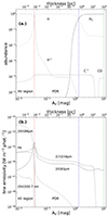 |
Fig. 2. Structure of the emission region: structure in abundances (a) and structure in line emissivity (b) as a function of the visual extinction AV and of the thickness for Z = 0.014, nH = 100 cm−2 and U = 10−3. The HII region is located at the left of the ionization front (vertical dashed red line), and the PDR and molecular region lie to its right. We stopped our simulation at AV = 10 (vertical dashed green line). |
We describe the line emission modeling of the effective HII regions and effective PDR in more detail before we add all terms of Eq. (1) together.
2.2. Nebular emission in HII regions
The galactic ISM converts the ionizing photons from the Lyman continuum photons into a continuum emission (free-free, free-bound, two-photon, and synchrotron emission) and into a series of emission lines (Osterbrock & Ferland 2006). The continuum and line emission can both be used to constrain the physical parameters of the emitting galaxy. The intensities of 160 atomic and molecular lines (H2 lines included) and of the nebular continuum emission originating from HII regions were computed using the photoionization code Cloudy, from the far-ultraviolet (FUV) to the millimeter range. This work has briefly been presented in Villa-Vélez et al. (2021). The HII region nebular continuum and emission lines fluxes depend on three parameters: the gas metallicity Zgas (see Sect. 2.2.3), the ionization radiation field intensity U (see Sect. 2.2.2), and the hydrogen density nH. The fluxes are given in [W phot−1], Watt per ionizing photon NLy, because we scale them below to the actual NLy to fit the global observed galaxy spectral energy distribution (SED; Boquien et al. 2019).
2.2.1. Definition of the effective HII region
The stopping criterion of the radiative transfer defines the size of the HII region and its emission volume, and therefore, the intensity of the lines. By choosing the ionization fraction ≤10−3, we have an ionization front located at ≃1 pc, depending on the chosen nH, Zgas, and U parameters. This stopping criterion implies that the effective HII region is radiation-bounded. With this choice, we ensured that the calculated line flux IHII originated from the HII region alone and not from the PDR or the molecular region.
2.2.2. Radiation field from the starburst region
The radiative response of the ISM to excitation by stellar light depends on the shape and the intensity of the stellar SED that is emitted by the ionizing stars or star cluster.
The shape of the radiation field was computed using:
-
The BC03 simple stellar population (SSP) library (Bruzual & Charlot 2003). The SSP library has two parameters: the stellar metallicity Zstar, and the age. The BC03 library only gives the stellar spectrum for six stellar metallicities Zstar.
-
The initial mass function (IMF) from Salpeter (1955) in the range: 0.1–100 M⊙.
-
A constant star formation rate (SFR) for 10 Myr. The age of the BC03 SSP can be varied, but we fixed it to 10 Myr (Kewley et al. 2001) because the SED does not vary significantly after 10 Myr.
The intensity of the photoionizing radiation field, the ionizing photons density NLy emitted by the stars (i.e., for wavelengths smaller than 91.2 nm) and impinging on the cloud, is also given by the chosen SSP, IMF, and SFH. It is commonly expressed by the dimensionless ionization parameter  , which represents the number density of H-ionizing photons to the number density of electrons (which equals the hydrogen density nH in the fully ionized medium of the HII region), and thus the competition between radiative ionization and neutralization. In the U parameter, the number density of H-ionizing photons and the matter density are correlated by definition. The ionization parameter U was varied in Cloudy from 10−4 to 10−1 by 0.1 dex, that is, 31 values. The stellar radiation field is by far the dominant ionization source in the HII regions. The cosmic-ray background was not included as an additional ionization source because cosmic rays affect HII regions very little.
2.2.3. Metallicity and initial atomic abundances
Our model uses the standard present-day metallicity scale, extended from the cosmic abundance standard and scaling developed by Nieva & Przybilla (2012), based on the observed metallicities of 29 early B-type stars in the local galactic region rather than the solar standard references. The solar abundances are relatively more uncertain, and the photospheric abundances do not reflect bulk or protosolar values (ca. 5 Gyr ago; Asplund et al. 2009; Grevesse et al. 2010; Lodders 2010). The choice of the cosmic abundance standard proposed by Nieva & Przybilla (2012) and the derivation of the element abundances was discussed in Nicholls et al. (2017). At the so-called local Galactic concordance, 12+log(O/H)GC = 8.76, which is close to the value 8.73 estimated for the protosolar solar abundance derived by Asplund et al. (2009) and Lodders (2010), and (O/H)GC = 5.76 × 10⁻⁴, (N/H)GC = 6.17 × 10⁻⁵, and ZGC = 0.01425. Following Nicholls et al. (2017), we introduce the ζO scaling parameter defined on the oxygen abundance:  . Thus, log ζO = 0 at the fiducial point (O/H)GC = 5.76 × 10⁻⁴, and log(ζO) < 0 for metal-poor galaxies. The depletion factors for each element were taken from Table 2 of Dopita et al. (2013). They are based on the Solar System depletion. The solid phase locked down into grains was not measured by Nieva & Przybilla (2012).
The abundance of helium increases steadily from its primordial value, the amount created through nucleosynthesis during the Big Bang, to the current value because helium is still being created continuously by stars. Fitting the abundance of helium observed in B stars by Nieva & Przybilla (2012), we derive the oxygen dependence of the helium abundance as
 (2)
(2)
The nitrogen-to-oxygen ratio (N/O) is of prime importance when building the nitrogen-based diagnostic diagram (Baldwin et al. 1981). Nevertheless, the nebular scaling of carbon and nitrogen with oxygen is a problem because oxygen is principally produced in core-collapse supernovae, while the carbon and nitrogen abundances both have a primary and secondary production mechanism (Vila-Costas & Edmunds 1993). The primary abundances originate from enrichment by core-collapse supernovae in the native gas cloud from which the emitting region formed, and the secondary abundances arise from delayed nucleosynthesis through hot-bottom burning and dredge-up in intermediate-mass stars as they evolve. Therefore, carbon and nitrogen were determined observationally (Nieva & Przybilla 2012; Dopita et al. 2013) and following Nicholls et al. (2017)
 (3)
(3)
 (4)
(4)
The evolution of the element abundances over cosmic times from the early Univesre to the present day, is a highly debated topic (Maiolino & Mannucci 2019), while also being an important parameter of line-emission modeling. The uncertainty on the (N/O) scaling affects the nitrogen abundance (N/H), which is seen in the difficulty to reproduce the [NII]λ6583/Hα ratio in BPT diagrams (Villa-Vélez et al. 2021). We chose to fix the (N/O) ratio using Eq. (4) and therefore did not use it as a free parameter, in contrast to other works (Morisset et al. 2016). Figure 3 gives the (N/O) and (C/O) prescriptions used in our models as a function of the oxygen abundance (O/H).
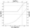 |
Fig. 3. N/O (solid-line) and C/O (dashed lines) abundance ratios as a function of O/H abundance. The dotted vertical and horizontal lines indicate the local Galactic concordance values of 12+log(O/H) and log(N/O). The ζO scaling parameter is displayed on the top horizontal axis. |
It is usual to simply scale the element abundances by a multiplicative factor related to Z, the mass fractions of all elements heavier than H and He, such as Z/Z⊙, where Z⊙ is the solar metallicity reference (Asplund et al. 2009; Grevesse et al. 2010; Lodders 2010). By summing the mass fraction of all the metals, it is possible to calculate the metallicity Zgas for each ζO. Table 1 gives the correspondence between the scaling based on the oxygen abundance and on the Zgas mass fraction.
Correspondence between ζO, the interstellar gas metallicities, and the stellar metallicities.
We disconnected the ISM gas-phase metallicity Zgas (or the corresponding ζO) from the stellar metallicity Zstar. The stars are expected to be as metallic as or less metallic than the ISM because they have formed from the previous surrounding ISM gas, which was later enriched (Bresolin et al. 2009, 2016; Hernandez et al. 2021). As discussed in Sect. 2.2.2, the photoionizing radiation field was derived from Bruzual & Charlot (2003) single stellar population synthesis, limited to only six stellar metallicities. To allow a finer description of the metallicity, we considered 26 gas metallicities Zgas, which are equal or nearly equal to the Zstar BC03 stellar metallicities according to Table 1. The emission line spectrum for a given gas metallicity ζO (or Zgas) was therefore calculated using the stellar radiation field of the corresponding Zstar (see Sect. 2.2.2).
We did not take depletion onto grains into account in our effective HII regions (dust-to-gas ratio is zero for any Zgas). The depletion of metals onto dust grains has traditionally not been taken into account in galactic HII regions either because dust is considered to have little effect on the emission spectrum (Mathis 1986), or it was taken into account with a slight correction with respect to oxygen abundance measurements (Mesa-Delgado & Esteban 2010; Peimbert & Peimbert 2010; Kewley et al. 2019), whereas observations of very small grains and big grains have been observed in local HII regions (Anderson et al. 2012). However, a galactic effective HII region is not the sum of HII regions with one star at the center, but rather a region of ionized gas with multiple youngs stars. Silicates and graphite have typical sublimation temperatures of 1500 K and 4000 K, respectively (Costa et al. 2017; Brewer et al. 1948), and their size and abundances distributions as well as their chemical composition are affected by the temperature and the radiation field (Kobayashi et al. 2011). Moreover, a radiative drift pushes dust outward the HII region of a particular star (Akimkin et al. 2015, 2017), possibly into the next neighboring HII region in starbust regions. Even if we modify the depletion factor changes the temperature structure in a HII region, and consequently, the intensity of several lines, it is beyond the scope of this paper to introduce different spatial and size distributions or chemical compositions. We simply directly used the second column of Table 2 for the abundances and ran dust-free models for the effective HII region.
Undepleted atomic abundances at ζO = 0.0 the local Galactic concordance reference value (ZGC = 0.0142) and depletion factor D adopted for each element.
We calculated the nebular continuum and line emissions for the 26 metallicities given in Table 1 and for three values of the hydrogen density nH: 10 cm−3, 100 cm−3, and 1000 cm−3.
2.2.4. Dust attenuation
We did not account for the grain extinction in the equivalent HII region during the Cloudy radiative transfer calculation because attenuation dominates galactic emission as a result of the dust/star distribution. The attenuation takes the extinction due to the grains and due to the geometry of the galaxy into account, the latter being dominant. The attenuation of the HII region lines is expressed by the gatt(λ) attenuation function in Eq. (1). The lines are screened with the Milky Way extinction law of Cardelli et al. (1989) with RV = 3.1, which is typical of diffuse media, and AV = 1, which is typical of a galaxy (Israel & Kennicutt 1980). We ran this oversimplified model for the attenuation law gatt(λ) for the consistency of the subsequent integration into CIGALE. A fixed AV = 1 precludes the comparison between optical and IR lines. However, the more elaborate treatment of both the stellar continuum and line attenuations with several recipes (Calzetti et al. 2000; Charlot & Fall 2000), variable AV, and variable E(B − V)continuum/E(B − V)lines allows this comparison. We can only compare IR lines between themselves here because gatt∼1 in the IR. We kept the (1 − fcov) light fraction in Eq. (1) for the sake of consistency, however.
2.3. Modeling the photodissociation and molecular regions
We modeled the second component of our two-sector model (see Sect. 2.1), the dense cloud that partially covering the effective HII region, as expressed in the second term of Eq. (1). The cloud after the ionization front exhibits both a PDR region and a molecular region.
2.3.1. Defining the size of the effective PDR region
The stopping criterion of the radiative transfer of the incoming radiation field within the interstellar matter defines the emission region and its size. Following the PDR code comparison by (Röllig et al. 2007), we set the stopping criterion to AV = 10. We thus defined an emission region that accounted for the totality of the PDR zone (delimited by the O/O2 transition) and a large part of the molecular region, for a thickness of ≃100 pc depending on the (nH, Zgas, U) set of parameters, as sketched in Fig. 2. Because we consider PDR lines here, it is important to obtain the full PDR zone. The thickness of the molecular regions is not as important.
2.3.2. The photodissociating radiation field
The photochemical equilibrium in the cloud has several drivers: (i.) the starburst region photodissociating radiation field exiting the effective HII region, (ii.) the cosmic-ray-induced secondary field, (iii.) the interstellar radiation field of nonionizing stars, and the (iv.) the cosmic background radiation. The last three sources are isotropic sources of photodissociation that is present everywhere in the cloud. The stellar radiation field from the effective HII region is the dominant source of photodissociation until it is damped. The average interstellar radiation field permeating the diffuse medium was not taken into account because we modeled the emission from the clouds in contact with the starburst emission zone. We need both the shape of the spectral energy distribution and the intensity of the photodissociating field that excites the atomic and molecular emission lines in the dense cloud.
The radiation field of the starburst region. After the ionization front, all the far-UV H-ionizing photons are lost with respect to the photoionizing radiation field entering the effective HII region. In Fig. 4 we compare (i.) the photoionizing radiation field illuminating the effective HII region, (ii.) the radiation field exiting the effective HII region, and (iii.) a photoionizing radiation field truncated at the Lyman break (91.2 nm) as a function of the (nH, Zstars, U) parameters.
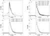 |
Fig. 4. Spectral energy distributon of the radiation field: at the entrance of the HII region (dotted line), at the ionization front (dashed line), compared to the same initial BC03 radiation field simply truncated at the Lyman break (solid line), (a) for log U = −2, nH = 100 cm−3 and Zstars = 0.02, (b) as a function of Zstars, (c) as a function of U for nH = 100 cm−3) and Zstars = 0.02, (d) and as a function of nH for log U = −2 and Zstars = 0.02. |
As shown in Fig. 4, the radiation field intensity U and the hydrogen density nH have only minor effects on the shape of the transmitted continuum from the effective HII region, while the metallicity affects this photodissociating radiation field slightly more (Fig. 4b). We note that a truncated initial photoionizing radiation field at the Lyman break is a good approximation of the stellar radiation field at the entrance of the PDR. Moreover, the nebular continuum emission is added to the truncated initial photoionizing radiation field. The line and continuum nebular emission produced by this field in the PDR, the IPDR term in Eq. (1), was calculated by subtracting the emission flux from the HII region + PDR (AV ≤ 10) from the emission flux from the HII region (ionization fraction ≤10−3) in the same physical and chemical conditions.
Cosmic rays. If in HII regions the radiation from the stars is by far the dominant source of ionization, cosmic rays take over as the ionization source in PDR and molecular regions. Cosmic rays ionize atoms and molecules and heat the gas to induce a rich ion-neutral chemistry (Herbst & Klemperer 1973) that causes the line emissions of molecular species such as  , H2O+, HCO+, ArH+, or OH+(Oka 2019; Neufeld & Wolfire 2017; Bacalla et al. 2019) in the molecular regions. In return, the abundance of these species is a probe of the cosmic-ray flux (Le Petit et al. 2016). Cosmic-ray ionization from the galactic background cosmic rays is included in the line emission calculations, and we took the default values of ζp = 2 × 10⁻¹⁶ s−1 for the mean H cosmic-ray ionization rate (Indriolo et al. 2007), we set the H secondary ionization rate to ζp = 2 × 10⁻¹⁷ s−1 (Röllig et al. 2007), and we took ζ2 = 4.6 × 10⁻¹⁶ s−1 for the H2 secondary ionization rate (Glassgold & Langer 1974). Nevertheless, several observations suggest that the ionization rate can be several times higher for the galactic ISM (McCall et al. 2003; Shaw et al. 2008; Muller et al. 2016; Bacalla et al. 2019) and orders of magnitude higher for starburst galaxies (Suchkov et al. 1993; Uzgil et al. 2016).
The interstellar radiation field. The interstellar radiation field is the average radiation field that permeates the diffuse medium originating from the nonionizing stars (red stars in Fig. 1). It would be the source of line excitation for a cloud that is not illuminated by the effective HII region. In our model, the photodissociating radiation field in the PDR is dominated by radiation from the neighboring star, and we therefore did not consider the interstellar radiation field.
Cosmic background radiation. The rest-frame cosmic background radiation (CBR) emits as a blackbody with TCMB = 2.73 K (1 + z) and can affect the intensities of fine-structure lines (Lagache et al. 2018). Because an inclusion of the CBR would mean that a redshift parameter in addition to (nH, Zgas, U) would need to be added, which is not supported by CIGALE at the moment, and because the CBR has a limited influence, ∼0.2 dex on the intensities on the [CII]158μm (Lagache et al. 2018) compared to other uncertainties, we did not include it as a radiation source here.
2.3.3. Interstellar matter and grains
In the PDR and molecular region, we treated the effects of the grains differently than in the HII region because the Calzetti law was not built for PDRs. We therefore performed a full radiative transfer to compute the IPDR term of Eq. (1), taking the effect of grains typical of the ISM into account. The grains have three main effects:
-
They deplete the gas phase from the refractory elements when the grain temperature is low enough. In a PDR, the grain temperature is a few dozen Kelvin. We therefore considered the depletion and used the depletion coefficients from Table 2.
-
They heat the gas by photoelectric effects, and they host a rich surface chemistry.
-
They absorb and scatter the light, and they cause the A(λ) extinction curve.
The extinction curve A(λ) depends on the grain properties: their chemical composition, size, and distribution (van Hoof et al. 2004). We chose to use grains with an appropriate size distribution and abundance to reproduce the observed overall extinction properties for the ISM of our Galaxy. This grain distribution included both a graphitic and a silicate component, and the ratio of extinction per reddening is RV ≡ AV/E(B − V) = 3.1 (van Hoof et al. 2004; Ferland et al. 2017). We also included PAHs in our modeling because they can heat the ISM and thus affect the line fluxes.
In our model, we did not propagate the emission lines created in the HII region through the PDR region and accounted for their extinction through the IHII × 10−A(λ) term of Eq. (1). To calculate this term for all the HII region emission lines, we need to know the A(λ) extinction curve. To derive this, we used Cloudy to perform a radiative transfer calculation of a spherical photodissociating radiation field, such as shown in Fig. 4, with the boundary condition AV ≡ A(550 nm) = 10 for the {nH, Zgas, U} set of parameters given in Table 3. We directly retrieved the extinction coefficient τ = τabs + τscatt, where τabs and τscatt are the grain absorption and scattering coefficients, respectively, and used A(λ) = 1.086 × τ(λ). We verified that NH = 1.85 × 1022 cm−2 when the radiative transfer stopped (AV = 10). We obtained the extinction curve displayed in Fig. 5. This extinction curve is similar to the curve from Wang & Chen (2019) for RV = 3.1.
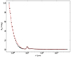 |
Fig. 5. Extinction curve in the PDR radiation field derived from the transmitted spectrum of a BC03 radiation field truncated at the Lyman break. The extinction at 550 nm is the boundary condition for the end of the PDR: AV = 10. The curve is fitted against two power-law functions and two Gaussian functions (dotted lines). |
Parameters we used to compute the nebular continuum and line emission.
In order to obtain an analytical expression of the A(λ) extinction curve, we fit it against two power laws and two Gaussian functions to obtain
![Mathematical equation: $$ \begin{aligned} \tiny A(\lambda [\upmu \mathrm{m}])={\left\{ \begin{array}{ll} -0.0188 + 10\times (\frac{\lambda }{0.550\,\upmu \mathrm{m}})^{-1.449} ,&\mathrm{if}\ \lambda < 7\, \upmu \mathrm{m}\\ -0.05 + 0.499\times \exp \left(\frac{\lambda - 9.79}{2\times 1.26^2}\right)&\\ + 0.27\times \exp \left(\frac{\lambda - 18.42}{2\times 7.5^2}\right) ,&\text{ if}\ 7 \,\upmu \mathrm{m} \le \lambda \le 24 \,\upmu \mathrm{m}\\ 0.00184 + 30.5\times \lambda ^{-1.638} ,&\text{ if}\ \lambda > 24\, \upmu \mathrm{m}. \end{array}\right.} \end{aligned} $$](/articles/aa/full_html/2024/02/aa47166-23/aa47166-23-eq8.gif) (5)
(5)
The two Gaussian functions account for the amorphous silicate SiO-stretching and OSiO-bending modes at 9.79 μm and 18.42 μm. They break the power-law extinction curves into two power laws. We did not consider weaker carbon or PAH features. The 12 resulting fit parameters are given in Tables A.1 and A.2. Figure 5 and Tables A.1 and A.2 show that the (Zgas, U, nH) set of parameters has a limited impact on the parameters. We therefore chose for Eq. (5) the set of final parameters that is summarized in the bottom lines of Tables A.1 and A.2 with their 1σ uncertainties to account for the extinction in all our PDR models. As shown in Fig. 5, AV = A(0.55 μm) = 10 from our choice of stopping conditions, the optical lines are almost extinguished and the near-IR lines are strongly attenuated.
2.3.4. Summary of the parameters for the effective HII region and effective PDR nebular emission
The line emission fluxes as expressed in Eq. (1) depend on several parameters. Table 3 summarizes the different input parameters we used to generate libraries of continuum and line emission spectra. IHII was obtained running Cloudy with the parameters and stopping conditions given in the column labeled “effective HII region” in Table 3. IPDR was obtained by running Cloudy twice, with the parameters given in the column labeled “effective PDR region”, first with the stopping condition defining the ionization front, and second with the stopping condition of AV = 10; IPDR is the subtraction of the latter from the former.
As explained above, several parameters were fixed. The hydrogen density, the metallicity, and the ionization parameter, {nH, Zgas, U}, were varied withing a certain range. The other parameters were fixed to specific values. A total of 2418 spectral libraries were generated for the different {nH, Zgas, U} parameters. They were provided to the CIGALE galaxy SED-fitting code.
3. Benchmarking with observations
To compare our models with observations, we used different samples both in the optical and in the IR taken from the literature. The simultaneous comparison of the observed strong optical and strong IR lines will be done in a future work using the CIGALE framework with a varying gatt, as explained in Sect. 2.2.4. In this study, we can only discuss strong IR lines that originate from either the HII region or the PDR. We used IR emission line ratios and IR emission line diagnostic diagrams. The line ratios prevent problems due to calibration issues, and well-chosen line ratios can be very instrumental in removing parameter degeneracies. The removal of dust attenuation effects offered by the line ratios that lie close in wavelength is not as interesting as it is for BPT diagrams (Baldwin et al. 1981) because the dust attenuation and extinction in the MIR and FIR is low (see Sects. 2.2.4 and 2.3.3).
3.1. Observation samples
A first sample was taken from the Herschel/PACS far-infrared line emission survey of local luminous infrared galaxies (LIRGs) presented in Díaz-Santos et al. (2017). In this sample, several fine-structure lines, [OI]63μm, [OIII]88μm, [N+]122μm, and [C+]158μm, are observed in the far-infrared (FIR) for ∼ 240 local LIRGs. We selected the 76 galaxies with detected lines. We refer to this sample as the great observatories all-sky LIRG survey (GOALS) sample.
Another sample consisted of the compilation of atomic fine-structure lines and molecular lines for 227 local galaxies reported in Brauher et al. (2008) using the ISO long-wavelength spectrometer. The most intense atomic lines ([OIII]52 μm, [NIII]57μm, [OI]63μm, [OIII]88μm, [N+]122μm, [OI]145μm, and [C+]158μm) are detected either in HII regions or PDRs at several locations in the same galaxies. We removed the upper limits in our sample. We refer to this sample as the ISO-LWS sample.
Another sample was taken from the Herschel Dwarf Galaxy Survey (DGS; Madden et al. 2013) selections of Cormier et al. (2019) and Ramambason et al. (2022), which gather photometric and spectroscopic observations of 42 nearby low-metallicity galaxies performed with the Herschel/PACS instrument in the FIR and with the Spitzer/IRS telescope in the MIR. The DGS sample exhibits a wide range of physical and chemical conditions. The interest of this sample lies in its low-metallicity ISM, which may resemble high-redshift galaxies, in the number of measured IR lines, and in the fact that many galaxies of this sample are also detected in the optical range. We refer to this sample as to the DGS sample.
The Survey with Herschel of the ISM in Nearby INfrared Galaxies (SHINING) sample consists of 52 local galaxies (z < 0.2) of different optical classification observed with Herschel/PACS. We took the integrated line fluxes from Table 6 of Herrera-Camus et al. (2018) for [NIII]57μm, [OI]63μm, [OIII]88μm, [NII]122μm, [OI]145μm, and [CII]158μm.
Another sample came from the KINGFISH local galaxy spectroscopic survey presented in Kennicutt et al. (2011) and Croxall et al. (2017), with measurements of [C+]158μm, [N+]122μm, and [N+]205μm line emission fluxes for 280 galaxies. The KINGFISH sample covers a wide range of galaxy properties and ISM environments and is therefore a good benchmark for our model. We obtained both IR and optical data ([OIII]500.7nm and Hα) for 20 galaxies when we cross-matched Croxall et al. (2017) and Moustakas et al. (2010) and added the [OIII]88μm fluxes published in Lamarche et al. (2022) for M101.
The sample of 16 galaxies taken from Boselli et al. (2002) combines IR and optical data for [C+]158μm and Hα (corrected for the N+ contribution). We did not take upper limits into account here either.
Finally, we also compiled a sample of high-redshift galaxies, including the compilation of De Looze et al. (2014) and the ALMA and NOEMA observations of Lagache et al. (2018), Harikane et al. (2020), Vanderhoof et al. (2022), Algera et al. (2023), and we added the Herschel/SPIRE-FTS observations of HLSW-01 of Rigopoulou et al. (2018) for a total of 143 galaxies with 0.6 ≤ z ≤ 9.1. This sample is not complete enough for IR line diagnostic diagrams, but it allowed us to investigate a few line ratios.
3.2. Line ratio diagnostics
Infrared line ratios can be used to ideally constrain the four parameters of our model (nH, Zgas, U, and fcov). A useful IR line ratio strongly varies with only one model parameter and allows us to constrain this parameter. When several line ratios are available, possible degeneracies between the parameters are lifted. For example, Rigopoulou et al. (2018) considered the [OIII]88μm/[N+]122μm line ratio as a potential diagnostic ratio of the gas-phase metallicity. The [OIII]88μm and [N+]122μm lines have similar critical densities of about 300–500 cm−3, and therefore, the ratio does not depend strongly on the model gas density. However, it strongly depends on the ionization parameter U because the number of available ionizing photons will strongly influence the relative amounts of O2+ and N+ gas. Nevertheless, the [OIII]88μm/[N+]122μm line ratio is interesting for high-redshift galaxies because both lines shift into the wavelength coverage of ALMA for galaxies at z > 5. Rigby & Rieke (2004) and Pereira-Santaella et al. (2017) explored several mid-IR ratios. Rigby & Rieke (2004) constrained the metallicity and IMF limit mass withe the He 2.06 μm/H Brγ or [Ne2+]15.6μm/[Ne+]12.8μm line ratios, and constrained the spectrum of the ionization ratio with the [S3+]10.5μm/(S2+18.7μm], [S3+]10.5μm/[Ne+]12.8μm or [Ne2+]15.6μm/[Ne+]12.8μm line ratios. Pereira-Santaella et al. (2017) found that the [S3+]10.5μm/[Ne2+]15.6μm ratio provides good constraints on the value of the ionization parameter, the [S2+]19μm/[S2+]33μm, [OIII]52μm/[OIII]88μm, or [N+]122μm/[N+]205μm ratios trace the density, and the [OIII]88μm/[N+]205μm, [OIII]52μm/[N+]122μm, and [OIII]52μm/[N+]205μm trace the metallicity. Herrera-Camus et al. (2016) reported that [OI]63μm/[CII]158μm traces the star formation rate, but because of the correlation with metallicity, it is difficult to exploit. Croxall et al. (2012) used the [C+]158μm/[N+]122μm and [C+]158μm/[N+]205μm line ratios to trace the density. Harikane et al. (2020) used the [OIII]88μm/[N+]122μm to trace the ionization parameter. We examine these line ratios as a function of the main model parameters in Appendix B.
We only study strong IR line ratios, especially from the IR lines in most of our samples. Some of the lines originate from the HII region alone, some from the PDR alone, and some from both the HII region and the PDR. We reproduce some of the ratios studies in previous work as a consistency check in Appendix B and propose below our best IR line ratios to trace the parameters. All the observations of our samples are covered by our models. The solution is clearly degenerate because several sets of parameters (nH, Zgas, U, fcov) can reproduce one IR line ratio. To remove this degeneracy, we independently fixed the parameters in a multiwavelength approach, either based on other IR line ratios or on optical line ratios. Fixing the best appropriate set of parameters for our effective HII region-PDR bisector model enables us to reliably predict the emission line fluxes in a consistent combined spectrophotometric approach because emission line ratios or individual lines fluxes can be related to galaxy evolution parameters, for example, the SFR-L([CII]158μm) or SFR-L([OIII]88μm) relations (De Looze et al. 2014; Lagache et al. 2018).
3.2.1. Tracers of the ionization parameter
The [OIII]88μm/[N+]122μm line ratio was proposed by Rigopoulou et al. (2018) to trace the ionization parameter, and it is shown in Fig. B.1, which corresponds to the fcov = 0 case. We investigated the [OIII]88μm/[N+]122μm line ratio as a function of the ionization parameter U dependence as a function of the ionization parameter for fcov = 0, 0.25, and 0.5, as displayed in Fig. 6. We note a weaker dependence on fcov in this ratio than in the [OIII]88μm/[OI]63μm line ratio.
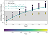 |
Fig. 6. [OIII]88μm/[N+]122μm line ratio as a function of the ionization parameter for three gas densities nH = 10 (circle), 100 (square), and 1000 (triangle) cm−3, and for different values of the metallicity Z = 0.0004, 0.004, 0.02, and 0.05 (from purple to yellow) for fcov = 0 (dotted line), 0.25 (dash-dotted line) and 0.5 (dashed line). The shaded region corresponds to the values spanned by this ratio in our samples. |
In addition to the [OIII]88μm/[N+]122μm line ratio, we propose to use the [OIII]88μm/[OI]63μm line ratio as a tracer of the ionization parameter, as shown in Fig. 7 because this ratio also traces the density, and the density and the ionization parameter are degenerate on these ratios. The [OIII]88μm/[OI]63μm line ratio is affected to a lesser extent by fcov, as shown for fcov = 0, 0.25, and 0.5.
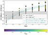 |
Fig. 7. [OIII]88μm/[OI]63μm line ratio as a function of the ionization parameter for three gas densities nH = 10 (circle), 100 (square), and 1000 (triangle) cm−3, for different values of the metallicity from 0.0001 to 0.05 (from purple to yellow), and for three covering factors fcov = 0 (dotted line), 0.25 (dash-dotted line), and 0.5 (dashed line). The shaded region corresponds to the values spanned by this ratio in our samples. |
3.2.2. Tracers of metallicity
To trace the metallicity, we propose to use the [OIII]88μm/[N+]122μm lines ratio, in agreement with Rigopoulou et al. (2018; see Appendix B). The dependences of this ratio on the density and covering factor are less pronounced than on Z. However, this line ratio is also sensitive to the ionization parameter (as previously shown in Fig. 6), introducing a correlation between Zgas and U.
Alternatively, we propose to use the [OIII]52μm/[C+]158μm (Fig. B.3) and the [OIII]52μm/ Paα or [OIII]88μm/ Paα line ratios (Figs. B.4 and B.5). Nevertheless, the dependence on the metallicity of these ratio is less marked.
3.2.3. Tracers of density
The density is probably the most difficult parameter to trace because line ratios are often also correlated to the metallicity and to the ionization parameter. In addition to the [C+]158μm/[N+]122μm and [C+]158μm/[N+]205μm line ratios proposed by Croxall et al. (2012) and to the [OIII]52μm/[OIII]88μm line ratio proposed by Pereira-Santaella et al. (2017), presented in Appendix B, we propose to use the [OIII]88μm/[OI]63μm and the [OIII]52μm/[C2+]158μm line ratios (see Figs. 8 and 9). In these figures (dotted lines), for a given set of (Zgas, U, fcov) when the density nH changes, the [C+]158μm/[N+]122μm, [OIII]52μm/[OIII]88μm, [OIII]88μm/[OI]63μm and the [OIII]52μm/[C2+]158 μm line ratios can vary by slightly more than one decade at best. These line ratios are dominantly affected by U and Zgas and to a lesser extent by fcov.
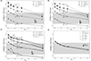 |
Fig. 8. [OIII]88μm/[OI]63μm line ratio as a function of the density for three different values of the metallicity, 0.004, 0.02, and 0.05 (from purple to yellow), and for different values of the ionization parameter, log U between −4.0 and −1.0 (with increasing size of the symbols), for fcov = 0 (HII region only). The shaded region corresponds to the values spanned by this ratio in our samples. |
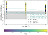 |
Fig. 9. [OIII]52μm/[C2+]158μm line ratio as a function of the density for three different values of the metallicity, 0.004, 0.02, and 0.05 (from purple to yellow), and for different values of the ionization parameter, log U between −4.0 and −1.0 (with increasing size of the symbols). The shaded region corresponds to the values spanned by this ratio in our samples. |
3.2.4. Tracers of the covering factor
In order to constrain the covering factor, we selected the ratios of lines, one of which originated mainly from HII regions, and the other from PDR (Spinoglio et al. 2017): [C+]158μm/[N+]122μm, [OIII]52μm/[OI]63μm, and [OIII]88μm/[OI]63μm, as displayed in Figs. 10–12, respectively. The first ratio also traces the density, and the other two ratios also trace the density and the ionization parameter. Again, the dependence on the ionization parameter is strong. For one set of (nH, Z and U), the line ratios can vary by more than one decade against the covering factor.
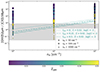 |
Fig. 10. [C+]158μm/[N+]122μm line ratio as a function of the covering factor for two gas densities nH = 10 (circle) and 1000 (triangle) cm−3 for different values of the metallicity from 0.0001 to 0.05 (from purple to yellow), and for different values of the ionization parameter, logU between −4.0 and −1.0 (with increasing size of the symbols). The shaded region corresponds to the values spanned by this ratio in our samples. |
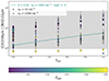 |
Fig. 11. [OIII]52μm/[OI]63μm line ratio as a function of the covering factor for three gas densities nH = 10 (circle), 100 (square), or 1000 (triangle) cm−3 for different values of the metallicity from 0.0001 to 0.05 (from purple to yellow), and for different values of the ionization parameter, log U between −4.0 and −1.0 (with increasing size of the symbols). The shaded region corresponds to the values spanned by this ratio in our samples. |
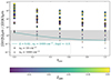 |
Fig. 12. [OIII]88μm/[OI]63μm line ratio as a function of the covering factor for three gas densities nH = 10 (circle), 100 (square), or 1000 (triangle) cm−3 for different values of the metallicity from 0.0001 to 0.05 (from purple to yellow), and for different values of the ionization parameter, log U between −4.0 and −1.0 (with increasing size of the symbols). The shaded region corresponds to the values spanned by this ratio in our samples. |
3.2.5. Summary of the line ratio diagnostic
Table 4 summarizes the parameters that are traced by a line ratio and also by which line ratios a parameter can be traced. Because of the degeneracy, a line ratio can trace several parameters (with a different degree of variation, here labeled weak, medium, and strong), and that a parameter can be traced by several line ratios. Globally, the variation with the ionization parameter U is dominant most of the time, the variation with metallicity is often strong, and the variation with the density nH and the covering factor fcov is less marked. This again points out the need to constrain the dominant parameters to constrain the others by using as many lines as possible, both in the optical and in the IR.
Summary of the different infrared diagnostic lines ratios and the parameters they trace (s: strong, m: medium, w: weak, –: no dependence).
3.3. 2D diagrams of the infrared emission line ratios
We showed in Sect. 3.2 that in all the proposed line ratios, all the parameters of our model (nH, Zgas, U, and fcov) are correlated. In order to break this correlation, we built IR line diagnostic 2D diagrams by combining two IR line ratios in the same way as optical line diagnostic diagrams are made (Baldwin et al. 1981). Locating observations in these diagrams provides a quick way to group galaxies and to determine their physical properties. As examples, Rigby & Rieke (2004) proposed the He 2.06 μm/H Brγ versus [Ne2+]15.6μm/[Ne+]12.8μm diagram, while De Breuck et al. (2019) showed that the [CII]158μm/[OI]145μm versus [OIII]88μm/[OI]145μm shows a trend in the PDR gas density, metallicity, and PDR covering fraction.
Because the [OIII]88μm/[OI]63μm ratio traces both the density and the ionization parameter (see Figs. 8 and 7) and because the [OIII]52μm/[OI]63μm tracies the covering factor (see Fig. 11), these two ratios might be combined in the [OIII]88μm/[OI]63μm versus [OIII]52μm/[OI]63μm IR diagram, hereafter, OOOO diagram. Because this diagram is made of four oxygen transitions (but with different ionization states), it is less sensitive to the metallicity, although the metallicity can change the temperatures of the different regions and can indirectly affect the temperature-dependent line ratios. However, this diagram is useless because it results in an almost linear relation between the [OIII]88μm/[OI]63μm and [OIII]52μm/[OI]63μm ratio because [OIII]88μm/[OI]63μm more strongly depends on the covering factor than on the density or ionization parameter.
3.3.1. The diagram of [C+]158μm/[OI]63μm versus [OIII]88μm/[N+]122μm (COON)
The diagram of [C+]158μm/[OI]63μm versus [OIII]88μm/[N+]122μm IR, hereafter COON diagram, is displayed in Fig. 13 along with our observation sample. It is composed of the ratio of two lines, [C+]158μm and [OI]63μm, which mainly originate from the PDR, and of two lines, [OIII]88μm and [N+]122μm, which mainly originate from HII regions (Spinoglio et al. 2017). By construction, this diagram is less sensitive to the covering factor and more sensitive to metallicity (different chemical elements), ionization parameter (different states of ionization), and density. Figure 13 shows the dependences on nH, Zgas and U for different coverage factors with arrows. The progression against U, indicated by lines, shows a clear pattern, and the density and metallicity procede in the opposite direction, the latter being dominant. Furthermore, the (nH, Zgas, U) pattern is shifted downward when the covering factor fcov increases; the covering factor and the metallicity are therefore anticorrelated. The metallicity trend between the ultraluminous IR galaxies (Díaz-Santos et al. 2017) and the low-metallicity galaxies (DGS; Madden et al. 2013) is respected. In agreement to what was observed in Sect. 3.2, our galaxy sample is best fit with low values of U or low metallicities for low PDR-covering factors and increasing values of U or increasing metallicities when the coverage increases. The offset due to the PDR-covering factor is strong at lower coverage and reduces as fcov increases. This means that for our galaxy sample, the PDR-covering factor is smaller than a half.
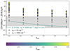 |
Fig. 13. [C+]158μm/[OI]63μm versus [OIII]88μm/[N+]122μm (COON) line emission diagram for three covering factors fcov = 0 (a), 0.5 (b), and 1 (c). Comparison of the different models against observations (GOALS (red), ISO-LWS (orange), and DGS (green)). The trends of the density nH, metallicity Z, ionization parameter U, and covering factor fcov are indicated by arrows. |
3.3.2. The diagram of [C+]158μm/[N+]122μm versus [OIII]88μm/[OI]63μm (CNOO)
The [C+]158μm/[N+]122μm versus [OIII]88μm/[OI]63μm diagram, hereafter CNOO diagram, as shown in Fig. 14, is composed of two ratios, [C+]158μm/[N+]122μm and [OIII]88μm/[OI]63μm, where one line mainly originates from a PDR and the other line from a HII region. In addition, the [OIII]88μm/[OI]63μm ratio is not directly sensitive to metallicity. Thus, by construction, this diagram is sensitive to the PDR/HII covering factor fcov. The dependences on the density, metallicity, ionization parameter, and covering factor are reported in Fig. 14. Similarly to the COON diagram, the ionization parameter shows a clear pattern, but this time, density and metallicity exhibit the same trend. The covering factor also shifts the whole pattern, but in an opposite way than density and metallicity. For our observations, low covering factors (fcov < 0.5) are again favored, consistent with what was found using the COON diagram.
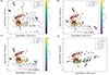 |
Fig. 14. [C+]158μm/[N+]122μm versus [OIII]88μm/[OI]63μm (CNOO) line emission diagram for three covering factors fcov = 0 (a), 0.5 (b), and 1 (c) and for five covering factors (d). Comparison of the different models (green) against observations (GOALS (red), ISO-LWS (orange), DGS (green)). The trends of the density nH, metallicity Z, ionization parameter U, and covering factor fcov are indicated by arrows. |
3.3.3. The diagram of [OIII]88μm/[NII]122μm versus [OIII]52μm/[OI]63μm (ONOO)
The [OIII]88μm/[NII]122μm versus [OIII]52μm/[OI]63μm IR diagram, hereafter ONOO diagram, as shown in Fig. 15, consists of the [OIII]88μm/[NII]122μm line ratio, which traces the metallicity (as it is particularly sensitive to the O/N ratio; see Fig. 16) and the ionization parameter (as shown in Fig. 6), and in the [OIII]52μm/[OI]63μm line ratio, which traces the covering factor (as shown in Fig. 11). Similarly to the OOOO diagram, the two line ratios are correlated strongly. However, this diagram is less sensitive to the density. Similarly to the other diagrams, the ionization parameter pattern is clear, and there is a strong change at low coverage that covers the observations better.
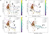 |
Fig. 15. [OIII]88μm/[NII]122μm versus [OIII]52μm/[OI]63μm (ONOO) diagram for three covering factors fcov = 0 (a), 0.5 (b), and 1 (c). Comparison of the different models (green) against observations (ISO-LWS (orange)). The trends of the density nH, metallicity Z, ionization parameter U, and covering factor fcov are indicated by arrows. |
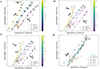 |
Fig. 16. [OIII]88μm/[N+]122μm line ratio as a function of the metallicity for three gas densities nH = 10 (circle), 100 (square), and 1000 (triangle) cm−3, for the ionization parameters log U varying betwen −4.0 and −1.0 (with increasing size of the symbols), and for the covering factor fcov = 0 (a), 0.5 (b), and 1 (c). The fcov = 0 case (a) corresponds to Fig. 5 of Rigopoulou et al. (2018). The shaded region corresponds to the values spanned by this ratio in our samples. |
4. Conclusion
We presented a bisector model to account for the density inhomogeneity of the ISM in external galaxies consistently and complementarily with previous HII region line emission modeling (Villa-Vélez et al. 2021). We introduced a dust-attenuated effective HII region that is partially covered by a dust-extincted effective PDR. Emission line fluxes are the sum of these two components, and they depend on several factors: the density, the metallicity, the ionization parameter, and the covering factor (nH, Z, U, and fcov). We reproduced previously published IR line ratios in the absence of PDR (fcov = 0), and we proposed several strong IR line ratio as diagnostics of our four model parameters. As expected, the four parameters are correlated, and the IR line ratios are degenerate. We also presented several 2D diagrams of strong IR line emission ratio, the [CII]158μm/[OI]63μm versus [OIII]88μm/[NII]122μm (COON) diagram, the [CII]158μm/[NII]122μm versus [OIII]88μm/[OI]63μm (CNOO) diagram, and the [OIII]88μm/[NII]122μm versus [OIII]52μm/[OI]63μm (ONOO) diagram. We benchmarked our model on several galactic spectroscopic surveys on several line ratios and located the galaxies of our samples in the different IR diagrams as a function of their physical properties. For our galaxy sample, we find low values for the ionization parameters and metallicities, which is consistent with what was derived previously. We also showed that low covering factors (fcov ≤ 0.5) are favored.
Although it is interesting at first to grasp the physics behind the IR emission line ratio and IR 2D diagrams, a reliable derivation of the parameters and their associated uncertainties requires statistical tools because of the degeneracy. We therefore computed the 160 line emission fluxes in the form of libraries, and these libraries were implemented in the CIGALE SED-fitting code (which is available upon request) as CIGALE provides a comprehensive consistent spectrophotometric SED-fitting tool using Bayesian statistics. The follow-up of this work is to fully and coherently constrain both the spectroscopy and the photometry of the galaxy SED from the far-ultraviolet to the radio using CIGALE in order to remove or at least estimate the degeneracy between the parameters. We will also investigate how the various SFR-Lline (SFR-L([CII]158μm) or SFR-L([OIII]88μm), e.g.) relations (De Looze et al. 2014; Lagache et al. 2018) are affected by the covering factor.
Acknowledgments
This work was supported by the Programme National ‘Physique et Chimie du Milieu Interstellaire’ (PCMI), by the Programme National ‘Cosmologie et Galaxies’ (PNCG) of CNRS/INSU with INC/INP and IN2P3, co-funded by CEA and CNES. P.T. would like to thank Christophe Morisset for his help on running Cloudy and PyCloudy.
References
- Akimkin, V. V., Kirsanova, M. S., Pavlyuchenkov, Y. N., & Wiebe, D. S. 2015, MNRAS, 449, 440 [NASA ADS] [CrossRef] [Google Scholar]
- Akimkin, V. V., Kirsanova, M. S., Pavlyuchenkov, Y. N., & Wiebe, D. S. 2017, MNRAS, 469, 630 [NASA ADS] [Google Scholar]
- Algera, H. S. B., Inami, H., Oesch, P. A., et al. 2023, MNRAS, 518, 6142 [Google Scholar]
- Anderson, L. D., Zavagno, A., Deharveng, L., et al. 2012, A&A, 542, A10 [NASA ADS] [CrossRef] [EDP Sciences] [Google Scholar]
- Asplund, M., Grevesse, N., Sauval, A. J., & Scott, P. 2009, ARA&A, 47, 481 [NASA ADS] [CrossRef] [Google Scholar]
- Bacalla, X. L., Linnartz, H., Cox, N. L. J., et al. 2019, A&A, 622, A31 [EDP Sciences] [Google Scholar]
- Baldwin, J. A., Phillips, M. M., & Terlevich, R. 1981, PASP, 93, 5 [Google Scholar]
- Beck, A., Lebouteiller, V., Madden, S. C., et al. 2022, A&A, 665, A85 [NASA ADS] [CrossRef] [EDP Sciences] [Google Scholar]
- Boquien, M., Burgarella, D., Roehlly, Y., et al. 2019, A&A, 622, A103 [NASA ADS] [CrossRef] [EDP Sciences] [Google Scholar]
- Boselli, A., Gavazzi, G., Lequeux, J., & Pierini, D. 2002, A&A, 385, 454 [NASA ADS] [CrossRef] [EDP Sciences] [Google Scholar]
- Brauher, J. R., Dale, D. A., & Helou, G. 2008, ApJS, 178, 280 [NASA ADS] [CrossRef] [Google Scholar]
- Bresolin, F., Gieren, W., Kudritzki, R.-P., et al. 2009, ApJ, 700, 309 [NASA ADS] [CrossRef] [Google Scholar]
- Bresolin, F., Kudritzki, R.-P., Urbaneja, M. A., et al. 2016, ApJ, 830, 64 [NASA ADS] [CrossRef] [Google Scholar]
- Brewer, L., Gilles, P. W., & Jenkins, F. A. 1948, J. Chem. Phys., 16, 797 [NASA ADS] [CrossRef] [Google Scholar]
- Bruzual, G., & Charlot, S. 2003, MNRAS, 344, 1000 [NASA ADS] [CrossRef] [Google Scholar]
- Burgarella, D., Buat, V., & Iglesias-Páramo, J. 2005, MNRAS, 360, 1413 [NASA ADS] [CrossRef] [Google Scholar]
- Burgarella, D., Theulé, P., Buat, V., et al. 2023, A&A, 671, A123 [NASA ADS] [CrossRef] [EDP Sciences] [Google Scholar]
- Calzetti, D., Armus, L., Bohlin, R. C., et al. 2000, ApJ, 533, 682 [NASA ADS] [CrossRef] [Google Scholar]
- Cardelli, J. A., Clayton, G. C., & Mathis, J. S. 1989, ApJ, 345, 245 [Google Scholar]
- Chabrier, G. 2003, PASP, 115, 763 [Google Scholar]
- Charlot, S., & Fall, S. M. 2000, ApJ, 539, 718 [Google Scholar]
- Cormier, D., Abel, N. P., Hony, S., et al. 2019, A&A, 626, A23 [NASA ADS] [CrossRef] [EDP Sciences] [Google Scholar]
- Costa, G. C. C., Jacobson, N. S., & Fegley, B., Jr. 2017, Icarus, 289, 42 [NASA ADS] [CrossRef] [Google Scholar]
- Croxall, K. V., Smith, J. D., Wolfire, M. G., et al. 2012, ApJ, 747, 81 [NASA ADS] [CrossRef] [Google Scholar]
- Croxall, K. V., Smith, J. D., Pellegrini, E., et al. 2017, ApJ, 845, 96 [Google Scholar]
- da Cunha, E., Charlot, S., & Elbaz, D. 2008, MNRAS, 388, 1595 [Google Scholar]
- De Breuck, C., Weiß, A., Béthermin, M., et al. 2019, A&A, 631, A167 [NASA ADS] [CrossRef] [EDP Sciences] [Google Scholar]
- De Looze, I., Cormier, D., Lebouteiller, V., et al. 2014, A&A, 568, A62 [NASA ADS] [CrossRef] [EDP Sciences] [Google Scholar]
- Díaz-Santos, T., Armus, L., Charmandaris, V., et al. 2017, ApJ, 846, 32 [Google Scholar]
- Dopita, M. A., Sutherland, R. S., Nicholls, D. C., Kewley, L. J., & Vogt, F. P. A. 2013, ApJS, 208, 10 [NASA ADS] [CrossRef] [Google Scholar]
- Ferland, G. J., Chatzikos, M., Guzmán, F., et al. 2017, Rev. Mex. Astron. Astrophys., 53, 385 [Google Scholar]
- Fitzgerald, K., Harvey, E. J., Keaveney, N., & Redman, M. P. 2020, Astron. Comput., 32, 100382 [CrossRef] [Google Scholar]
- Galliano, F., Madden, S. C., Jones, A. P., et al. 2003, A&A, 407, 159 [NASA ADS] [CrossRef] [EDP Sciences] [Google Scholar]
- Glassgold, A. E., & Langer, W. D. 1974, ApJ, 193, 73 [NASA ADS] [CrossRef] [Google Scholar]
- Grevesse, N., Asplund, M., Sauval, A. J., & Scott, P. 2010, Ap&SS, 328, 179 [Google Scholar]
- Groves, B., Dopita, M. A., Sutherland, R. S., et al. 2008, ApJS, 176, 438 [NASA ADS] [CrossRef] [Google Scholar]
- Harikane, Y., Ouchi, M., Inoue, A. K., et al. 2020, ApJ, 896, 93 [Google Scholar]
- Herbst, E., & Klemperer, W. 1973, ApJ, 185, 505 [Google Scholar]
- Hernandez, S., Aloisi, A., James, B. L., et al. 2021, ApJ, 908, 226 [NASA ADS] [CrossRef] [Google Scholar]
- Herrera-Camus, R., Bolatto, A., Smith, J. D., et al. 2016, ApJ, 826, 175 [Google Scholar]
- Herrera-Camus, R., Sturm, E., Graciá-Carpio, J., et al. 2018, ApJ, 861, 94 [Google Scholar]
- Indriolo, N., Geballe, T. R., Oka, T., & McCall, B. J. 2007, ApJ, 671, 1736 [NASA ADS] [CrossRef] [Google Scholar]
- Israel, F., & Kennicutt, R. 1980, Astrophys. Lett., 21, 1 [Google Scholar]
- Johnson, B. D., Leja, J., Conroy, C., & Speagle, J. S. 2021, ApJS, 254, 22 [NASA ADS] [CrossRef] [Google Scholar]
- Kennicutt, R. C., Calzetti, D., Aniano, G., et al. 2011, PASP, 123, 1347 [Google Scholar]
- Kewley, L. J., Dopita, M. A., Sutherland, R. S., Heisler, C. A., & Trevena, J. 2001, ApJ, 556, 121 [Google Scholar]
- Kewley, L. J., Nicholls, D. C., & Sutherland, R. S. 2019, ARA&A, 57, 511 [Google Scholar]
- Kobayashi, H., Kimura, H., Watanabe, S.-i., Yamamoto, T., & Müller, S. 2011, Earth Planets Space, 63, 1067 [NASA ADS] [CrossRef] [Google Scholar]
- Lagache, G., Cousin, M., & Chatzikos, M. 2018, A&A, 609, A130 [NASA ADS] [CrossRef] [EDP Sciences] [Google Scholar]
- Lamarche, C., Smith, J. D., Kreckel, K., et al. 2022, ApJ, 925, 194 [NASA ADS] [CrossRef] [Google Scholar]
- Le Petit, F., Ruaud, M., Bron, E., et al. 2016, A&A, 585, A105 [NASA ADS] [CrossRef] [EDP Sciences] [Google Scholar]
- Lodders, K. 2010, Astrophys. Space Sci. Proc., 16, 379 [NASA ADS] [CrossRef] [Google Scholar]
- Madden, S. C., Rémy-Ruyer, A., Galametz, M., et al. 2013, PASP, 125, 600 [NASA ADS] [CrossRef] [Google Scholar]
- Maiolino, R., & Mannucci, F. 2019, A&ARv, 27, 3 [Google Scholar]
- Mathis, J. S. 1986, PASP, 98, 995 [NASA ADS] [CrossRef] [Google Scholar]
- McCall, B. J., Huneycutt, A. J., Saykally, R. J., et al. 2003, Nature, 422, 500 [CrossRef] [Google Scholar]
- Mesa-Delgado, A., & Esteban, C. 2010, MNRAS, 405, 2651 [NASA ADS] [Google Scholar]
- Morisset, C., Delgado-Inglada, G., Sánchez, S. F., et al. 2016, A&A, 594, A37 [NASA ADS] [CrossRef] [EDP Sciences] [Google Scholar]
- Moustakas, J., Kennicutt, R. C. Jr., Tremonti, C. A., et al. 2010, ApJS, 190, 233 [NASA ADS] [CrossRef] [Google Scholar]
- Muller, S., Müller, H. S. P., Black, J. H., et al. 2016, A&A, 595, A128 [NASA ADS] [CrossRef] [EDP Sciences] [Google Scholar]
- Nagao, T., Maiolino, R., Marconi, A., & Matsuhara, H. 2011, A&A, 526, A149 [NASA ADS] [CrossRef] [EDP Sciences] [Google Scholar]
- Neufeld, D. A., & Wolfire, M. G. 2017, ApJ, 845, 163 [Google Scholar]
- Nicholls, D. C., Sutherland, R. S., Dopita, M. A., Kewley, L. J., & Groves, B. A. 2017, MNRAS, 466, 4403 [Google Scholar]
- Nieva, M. F., & Przybilla, N. 2012, A&A, 539, A143 [NASA ADS] [CrossRef] [EDP Sciences] [Google Scholar]
- Noll, S., Burgarella, D., Giovannoli, E., et al. 2009, A&A, 507, 1793 [NASA ADS] [CrossRef] [EDP Sciences] [Google Scholar]
- Oka, T. 2019, Phil. Trans. R. Soc. London, Ser. A, 377, 20180402 [Google Scholar]
- Osterbrock, D. E., & Ferland, G. J. 2006, Astrophysics of Gaseous Nebulae and Active Galactic Nuclei (University Science Books) [Google Scholar]
- Peimbert, A., & Peimbert, M. 2010, ApJ, 724, 791 [NASA ADS] [CrossRef] [Google Scholar]
- Péquignot, D. 2008, A&A, 478, 371 [NASA ADS] [CrossRef] [EDP Sciences] [Google Scholar]
- Pereira-Santaella, M., Rigopoulou, D., Farrah, D., Lebouteiller, V., & Li, J. 2017, MNRAS, 470, 1218 [NASA ADS] [CrossRef] [Google Scholar]
- Piovan, L., Tantalo, R., & Chiosi, C. 2006, MNRAS, 370, 1454 [CrossRef] [Google Scholar]
- Ramambason, L., Lebouteiller, V., Bik, A., et al. 2022, A&A, 667, A35 [NASA ADS] [CrossRef] [EDP Sciences] [Google Scholar]
- Rigby, J. R., & Rieke, G. H. 2004, ApJ, 606, 237 [NASA ADS] [CrossRef] [Google Scholar]
- Rigopoulou, D., Pereira-Santaella, M., Magdis, G. E., et al. 2018, MNRAS, 473, 20 [NASA ADS] [CrossRef] [Google Scholar]
- Röllig, M., Abel, N. P., Bell, T., et al. 2007, A&A, 467, 187 [Google Scholar]
- Salpeter, E. E. 1955, ApJ, 121, 161 [Google Scholar]
- Schaerer, D., Ginolfi, M., Béthermin, M., et al. 2020, A&A, 643, A3 [NASA ADS] [CrossRef] [EDP Sciences] [Google Scholar]
- Shaw, G., Ferland, G. J., Srianand, R., et al. 2008, ApJ, 675, 405 [NASA ADS] [CrossRef] [Google Scholar]
- Siebenmorgen, R., & Krügel, E. 2007, A&A, 461, 445 [NASA ADS] [CrossRef] [EDP Sciences] [Google Scholar]
- Spinoglio, L., Alonso-Herrero, A., Armus, L., et al. 2017, PASA, 34, e057 [NASA ADS] [CrossRef] [Google Scholar]
- Suchkov, A., Allen, R. J., & Heckman, T. M. 1993, ApJ, 413, 542 [NASA ADS] [CrossRef] [Google Scholar]
- Uzgil, B. D., Bradford, C. M., Hailey-Dunsheath, S., Maloney, P. R., & Aguirre, J. E. 2016, ApJ, 832, 209 [CrossRef] [Google Scholar]
- Vanderhoof, B. N., Faisst, A. L., Shen, L., et al. 2022, MNRAS, 511, 1303 [NASA ADS] [CrossRef] [Google Scholar]
- van Hoof, P. A. M., Weingartner, J. C., Martin, P. G., Volk, K., & Ferland, G. J. 2004, MNRAS, 350, 1330 [NASA ADS] [CrossRef] [Google Scholar]
- Vila-Costas, M. B., & Edmunds, M. G. 1993, MNRAS, 265, 199 [NASA ADS] [CrossRef] [Google Scholar]
- Villa-Vélez, J. A., Buat, V., Theulé, P., Boquien, M., & Burgarella, D. 2021, A&A, 654, A153 [NASA ADS] [CrossRef] [EDP Sciences] [Google Scholar]
- Wang, S., & Chen, X. 2019, ApJ, 877, 116 [Google Scholar]
- Williams, C. C., Tacchella, S., Maseda, M. V., et al. 2023, ApJS, 268, 64 [NASA ADS] [CrossRef] [Google Scholar]
Appendix A: The extinction curve A(λ) in the PDR
In order to obtain an analytical expression of the A(λ) extinction curve, we fit it against two power laws and two Gaussian functions at wavelength intervals [550 nm- 7μm], [7 μm- 24μm], and [24μm - 1.6 mm] with the equation
![Mathematical equation: $$ \begin{aligned} A(\lambda )&= [b_\mathrm{1} +10\times (\frac{\lambda }{550~nm})^{\delta 1}]\nonumber \\&+[c + A_\mathrm{1} \times \exp (\frac{\lambda - \lambda _\mathrm{1} }{2\sigma _1^2})+ A_\mathrm{2} \times \exp (\frac{\lambda - \lambda _\mathrm{2} }{2\sigma _\mathrm{2} ^2})]\\&+ [b_\mathrm{2} + A(14~\mu m)\times \lambda ^{\delta 2}].\nonumber \end{aligned} $$](/articles/aa/full_html/2024/02/aa47166-23/aa47166-23-eq9.gif) (A.1)
(A.1)
The two Gaussian functions account for the amorphous silicate SiO-stretching and OSiO-bending modes at 10 μm and 20 μm. They break the power-law extinction curves into two power laws. We did not consider weaker carbon or PAH features. The 12 resulting fit parameters are given in Tables A.1 and A.2. Fig. 5 and Tables A.1 and A.2 showed that the (nH, Z, U) set of parameters has a limited impact on the parameters. We therefore chose one set of final parameters, summarized at the bottom lines of Table A.1 and A.2 with their 1σ uncertainties, to account for the extinction in all our PDR models. We therefore obtain
![Mathematical equation: $$ \begin{aligned} A(\lambda [nm])&= -0.0188 + 10\times (\frac{\lambda }{550~nm})^{-1.449})\nonumber \\&-0.05 + 0.499\times \exp (\frac{\lambda - 9.79\mu m}{2\times (1.26\mu m^{-2})^2})\\&+ 0.27\times \exp (\frac{\lambda - 18.42\mu m}{2\times (7.5\mu m^{-2})^2})]\nonumber \\&-110~10^{-5} + 2.5~10^6\times \lambda ^{-1.645}\nonumber \end{aligned} $$](/articles/aa/full_html/2024/02/aa47166-23/aa47166-23-eq10.gif) (A.2)
(A.2)
Fit parameters of the extinction curve with their 1σ uncertainties
Fit parameters of the extinction curve with their 1σ uncertainties (continue)
Appendix B: Line ratio diagnostics
We reproduce in this appendix several of the line ratios and their dependences on the (nH, Zgas, U, and fcov) set of parameters as a consistency check with previously published work, as discussed in Section 3.2.
The ionization parameter can be traced by the [OIII]88 μm/[N+]122 μm line ratio (Fig. B.1), as shown in Fig. 17 and Fig.4 of Rigopoulou et al. (2018). The degeneracy betwen Zgas and U is again clear.
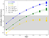 |
Fig. B.1. [OIII]88 μm/[N+]122 μm line ratio as a function of the ionization parameter for three gas densities nH = 10 (circle), 100 (square), and 1000 (triangle) cm−3, and for different values of the metallicity Z = 0.0004, 0.004, 0.02, and 0.05 (from purple to yellow) for fcov = 0. The shaded region corresponds to the values spanned by this ratio in our samples. |
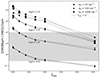 |
Fig. B.2. [OIII]88μm/[NII]122μm line ratio as a function of metallicity for three gas densities, nH = 10 (circle), 100 (square), or 1000 (triangle) cm−3, and different values of the ionization parameter, logU betwen -4.0 and -1.0 (with increasing size of the symbols), for fcov = 0. The shaded region corresponds to the values spanned by this ratio in our samples. |
The [OIII]88 μm/[N+]122 μm line ratio is sensitive to the metallicity ( Fig. ), as shown in Fig. 5 of Rigopoulou et al. (2018), and it does not depend strongly on the density. However, this line ratio is also sensitive to the ionization parameter B.1, which introduces a correlation between Zgas and U.
The metallicity can also be traced by the [OIII]52 μm/[C+]158 μm ( Fig. B.3) and the [OIII]52 μm/ Paα or [OIII]88 μm/ Paα line ratios (Fig. B.4 and B.5). The first ratio may be affected by the dependence of the [C+]158 μm emission line on fcov (see Fig. 2) and is sensitive to the choice of the O/N abundance ratio (see Eq. 4). The two last ratios, making use of the hydrogen Paschen alpha line, have the advantage to be closer to the (O/H) definition of the metallicity, as expressed by the ζO parameter (Nicholls et al. 2017) (see Section 2.2.3). The hydrogen Paschen alpha line can be observed and related to the galaxy star formation rate (Williams et al. 2023), but the ratios are sensitive to the choice of the extinction curve A(λ) (Appendix ). All these ratios vary by about one decade when the metallictiy changes for a particular set of (nH, U, and fcov) (visualized by the dotted line in Fig. B.3, B.4 and B.5). Similarly to the [OIII]88 μm/[N+]122 μm line ratio (see Fig. 16), the ionization parameter varies strongly, which needs to be constrained independently, and the density and covering factor vary more weakly.
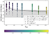 |
Fig. B.3. [OIII]52 μm/[C+]158 μm line ratio as a function of the gas metallicity Zgas for three gas densities nH = 10 (circle), 100 (square), and 1000 (triangle) cm−3, and for different values of the ionization parameter, logU between -4.0 and -1.0 (with increasing size of the symbols), for fcov = 0 (HII region only). The shaded region corresponds to the values spanned by this ratio in our samples. |
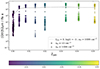 |
Fig. B.4. [OIII]52 μm/Paα line ratio as a function of the gas metallicity Zgas for three gas densities nH = 10 (circle), 100 (square), and 1000 (triangle) cm−3, and for different values of the ionization parameter, logU betwen -4.0 and -1.0 (with increasing size of the symbols), for fcov = 0 (HII region only). |
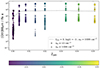 |
Fig. B.5. [OIII]88 μm/Paα line ratio as a function of the gas metallicity Zgas for three gas densities nH = 10 (circle), 100 (square), and 1000 (triangle) cm−3, and for different values of the ionization parameter, logU betwen -4.0 and -1.0 (with increasing size of the symbols), for fcov = 0 (HII region only). |
The density can be traced by either the [OIII]52 μm/[OIII]88 μm line ratio (Fig. B.6), as shown in Fig.1 of Pereira-Santaella et al. (2017) and in (Beck et al. 2022), or by the [C+]158 μm/[N+]122 μm line ratio (Fig. B.7), as shown in Fig.11 of Croxall et al. (2012). The density can also be traced by the ratios [SIII]19μm/[SIII]33μm and [N+]122μm/[N+]205μm (Beck et al. 2022). These three ratios have the advantage of being independent of the metallicity and ionization parameter.
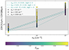 |
Fig. B.6. [OIII]52 μm/[OIII]88 μm line ratio as a function of the density for three different values of the metallicity, 0.004, 0.02, and 0.05 (from purple to yellow), and for different values of the ionization parameter, logU betwen -4.0 and -1.0 (with increasing size of the symbols), for fcov = 0. The shaded region corresponds to the values spanned by this ratio in our samples. |
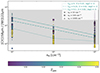 |
Fig. B.7. [C+]158 μm/[N+]122 μm line ratio as a function of the density for three different values of the metallicity, 0.004, 0.02, and 0.05 (from purple to yellow), and for different values of the ionization parameter, logU betwen -4.0 and -1.0 (with increasing size of the symbols), for fcov = 0. The shaded region corresponds to the values spanned by this ratio in our samples. |
All Tables
Correspondence between ζO, the interstellar gas metallicities, and the stellar metallicities.
Undepleted atomic abundances at ζO = 0.0 the local Galactic concordance reference value (ZGC = 0.0142) and depletion factor D adopted for each element.
Summary of the different infrared diagnostic lines ratios and the parameters they trace (s: strong, m: medium, w: weak, –: no dependence).
All Figures
|
Fig. 1. Scheme of our two-sector model. In a galaxy, starbust regions (blue stars) emit radiation that passes an equivalent HII region (blue zone) that is partially covered by clouds (red regions). They are modeled as a photodissociation region and a molecular region. We do not consider nebular emission from old stars (red stars). One part of the emission line flux directly moves from the HII region to the observer and is attenuated by galactic dust. A second part is attenuated within the PDR, and a third part is created inside the PDR. This is not the actual geometry used in Cloudy simulations, which are performed for a slab of gas that is illuminated by a starburst-region radiation field, as described in Sect. 2.2.2. |
| In the text | |
|
Fig. 2. Structure of the emission region: structure in abundances (a) and structure in line emissivity (b) as a function of the visual extinction AV and of the thickness for Z = 0.014, nH = 100 cm−2 and U = 10−3. The HII region is located at the left of the ionization front (vertical dashed red line), and the PDR and molecular region lie to its right. We stopped our simulation at AV = 10 (vertical dashed green line). |
| In the text | |
|
Fig. 3. N/O (solid-line) and C/O (dashed lines) abundance ratios as a function of O/H abundance. The dotted vertical and horizontal lines indicate the local Galactic concordance values of 12+log(O/H) and log(N/O). The ζO scaling parameter is displayed on the top horizontal axis. |
| In the text | |
|
Fig. 4. Spectral energy distributon of the radiation field: at the entrance of the HII region (dotted line), at the ionization front (dashed line), compared to the same initial BC03 radiation field simply truncated at the Lyman break (solid line), (a) for log U = −2, nH = 100 cm−3 and Zstars = 0.02, (b) as a function of Zstars, (c) as a function of U for nH = 100 cm−3) and Zstars = 0.02, (d) and as a function of nH for log U = −2 and Zstars = 0.02. |
| In the text | |
|
Fig. 5. Extinction curve in the PDR radiation field derived from the transmitted spectrum of a BC03 radiation field truncated at the Lyman break. The extinction at 550 nm is the boundary condition for the end of the PDR: AV = 10. The curve is fitted against two power-law functions and two Gaussian functions (dotted lines). |
| In the text | |
|
Fig. 6. [OIII]88μm/[N+]122μm line ratio as a function of the ionization parameter for three gas densities nH = 10 (circle), 100 (square), and 1000 (triangle) cm−3, and for different values of the metallicity Z = 0.0004, 0.004, 0.02, and 0.05 (from purple to yellow) for fcov = 0 (dotted line), 0.25 (dash-dotted line) and 0.5 (dashed line). The shaded region corresponds to the values spanned by this ratio in our samples. |
| In the text | |
|
Fig. 7. [OIII]88μm/[OI]63μm line ratio as a function of the ionization parameter for three gas densities nH = 10 (circle), 100 (square), and 1000 (triangle) cm−3, for different values of the metallicity from 0.0001 to 0.05 (from purple to yellow), and for three covering factors fcov = 0 (dotted line), 0.25 (dash-dotted line), and 0.5 (dashed line). The shaded region corresponds to the values spanned by this ratio in our samples. |
| In the text | |
|
Fig. 8. [OIII]88μm/[OI]63μm line ratio as a function of the density for three different values of the metallicity, 0.004, 0.02, and 0.05 (from purple to yellow), and for different values of the ionization parameter, log U between −4.0 and −1.0 (with increasing size of the symbols), for fcov = 0 (HII region only). The shaded region corresponds to the values spanned by this ratio in our samples. |
| In the text | |
|
Fig. 9. [OIII]52μm/[C2+]158μm line ratio as a function of the density for three different values of the metallicity, 0.004, 0.02, and 0.05 (from purple to yellow), and for different values of the ionization parameter, log U between −4.0 and −1.0 (with increasing size of the symbols). The shaded region corresponds to the values spanned by this ratio in our samples. |
| In the text | |
|
Fig. 10. [C+]158μm/[N+]122μm line ratio as a function of the covering factor for two gas densities nH = 10 (circle) and 1000 (triangle) cm−3 for different values of the metallicity from 0.0001 to 0.05 (from purple to yellow), and for different values of the ionization parameter, logU between −4.0 and −1.0 (with increasing size of the symbols). The shaded region corresponds to the values spanned by this ratio in our samples. |
| In the text | |
|
Fig. 11. [OIII]52μm/[OI]63μm line ratio as a function of the covering factor for three gas densities nH = 10 (circle), 100 (square), or 1000 (triangle) cm−3 for different values of the metallicity from 0.0001 to 0.05 (from purple to yellow), and for different values of the ionization parameter, log U between −4.0 and −1.0 (with increasing size of the symbols). The shaded region corresponds to the values spanned by this ratio in our samples. |
| In the text | |
|
Fig. 12. [OIII]88μm/[OI]63μm line ratio as a function of the covering factor for three gas densities nH = 10 (circle), 100 (square), or 1000 (triangle) cm−3 for different values of the metallicity from 0.0001 to 0.05 (from purple to yellow), and for different values of the ionization parameter, log U between −4.0 and −1.0 (with increasing size of the symbols). The shaded region corresponds to the values spanned by this ratio in our samples. |
| In the text | |
|
Fig. 13. [C+]158μm/[OI]63μm versus [OIII]88μm/[N+]122μm (COON) line emission diagram for three covering factors fcov = 0 (a), 0.5 (b), and 1 (c). Comparison of the different models against observations (GOALS (red), ISO-LWS (orange), and DGS (green)). The trends of the density nH, metallicity Z, ionization parameter U, and covering factor fcov are indicated by arrows. |
| In the text | |
|
Fig. 14. [C+]158μm/[N+]122μm versus [OIII]88μm/[OI]63μm (CNOO) line emission diagram for three covering factors fcov = 0 (a), 0.5 (b), and 1 (c) and for five covering factors (d). Comparison of the different models (green) against observations (GOALS (red), ISO-LWS (orange), DGS (green)). The trends of the density nH, metallicity Z, ionization parameter U, and covering factor fcov are indicated by arrows. |
| In the text | |
|
Fig. 15. [OIII]88μm/[NII]122μm versus [OIII]52μm/[OI]63μm (ONOO) diagram for three covering factors fcov = 0 (a), 0.5 (b), and 1 (c). Comparison of the different models (green) against observations (ISO-LWS (orange)). The trends of the density nH, metallicity Z, ionization parameter U, and covering factor fcov are indicated by arrows. |
| In the text | |
|
Fig. 16. [OIII]88μm/[N+]122μm line ratio as a function of the metallicity for three gas densities nH = 10 (circle), 100 (square), and 1000 (triangle) cm−3, for the ionization parameters log U varying betwen −4.0 and −1.0 (with increasing size of the symbols), and for the covering factor fcov = 0 (a), 0.5 (b), and 1 (c). The fcov = 0 case (a) corresponds to Fig. 5 of Rigopoulou et al. (2018). The shaded region corresponds to the values spanned by this ratio in our samples. |
| In the text | |
|
Fig. B.1. [OIII]88 μm/[N+]122 μm line ratio as a function of the ionization parameter for three gas densities nH = 10 (circle), 100 (square), and 1000 (triangle) cm−3, and for different values of the metallicity Z = 0.0004, 0.004, 0.02, and 0.05 (from purple to yellow) for fcov = 0. The shaded region corresponds to the values spanned by this ratio in our samples. |
| In the text | |
|
Fig. B.2. [OIII]88μm/[NII]122μm line ratio as a function of metallicity for three gas densities, nH = 10 (circle), 100 (square), or 1000 (triangle) cm−3, and different values of the ionization parameter, logU betwen -4.0 and -1.0 (with increasing size of the symbols), for fcov = 0. The shaded region corresponds to the values spanned by this ratio in our samples. |
| In the text | |
|
Fig. B.3. [OIII]52 μm/[C+]158 μm line ratio as a function of the gas metallicity Zgas for three gas densities nH = 10 (circle), 100 (square), and 1000 (triangle) cm−3, and for different values of the ionization parameter, logU between -4.0 and -1.0 (with increasing size of the symbols), for fcov = 0 (HII region only). The shaded region corresponds to the values spanned by this ratio in our samples. |
| In the text | |
|
Fig. B.4. [OIII]52 μm/Paα line ratio as a function of the gas metallicity Zgas for three gas densities nH = 10 (circle), 100 (square), and 1000 (triangle) cm−3, and for different values of the ionization parameter, logU betwen -4.0 and -1.0 (with increasing size of the symbols), for fcov = 0 (HII region only). |
| In the text | |
|
Fig. B.5. [OIII]88 μm/Paα line ratio as a function of the gas metallicity Zgas for three gas densities nH = 10 (circle), 100 (square), and 1000 (triangle) cm−3, and for different values of the ionization parameter, logU betwen -4.0 and -1.0 (with increasing size of the symbols), for fcov = 0 (HII region only). |
| In the text | |
|
Fig. B.6. [OIII]52 μm/[OIII]88 μm line ratio as a function of the density for three different values of the metallicity, 0.004, 0.02, and 0.05 (from purple to yellow), and for different values of the ionization parameter, logU betwen -4.0 and -1.0 (with increasing size of the symbols), for fcov = 0. The shaded region corresponds to the values spanned by this ratio in our samples. |
| In the text | |
|
Fig. B.7. [C+]158 μm/[N+]122 μm line ratio as a function of the density for three different values of the metallicity, 0.004, 0.02, and 0.05 (from purple to yellow), and for different values of the ionization parameter, logU betwen -4.0 and -1.0 (with increasing size of the symbols), for fcov = 0. The shaded region corresponds to the values spanned by this ratio in our samples. |
| In the text | |
Current usage metrics show cumulative count of Article Views (full-text article views including HTML views, PDF and ePub downloads, according to the available data) and Abstracts Views on Vision4Press platform.
Data correspond to usage on the plateform after 2015. The current usage metrics is available 48-96 hours after online publication and is updated daily on week days.
Initial download of the metrics may take a while.