| Issue |
A&A
Volume 666, October 2022
|
|
|---|---|---|
| Article Number | A142 | |
| Number of page(s) | 22 | |
| Section | Catalogs and data | |
| DOI | https://doi.org/10.1051/0004-6361/202244037 | |
| Published online | 19 October 2022 | |
Periodic variable A-F spectral type stars in the northern TESS continuous viewing zone
I. Identification and classification★
1
Astronomical Institute of the Czech Academy of Sciences,
Fričova 298,
25165
Ondřejov, Czech Republic
e-mail: This email address is being protected from spambots. You need JavaScript enabled to view it.
2
Department of Theoretical Physics and Astrophysics, Masaryk University,
Kotlářská 2,
61137
Brno, Czech Republic
3
Variable Star and Exoplanet Section of the Czech Astronomical Society,
Vsetinská 941/78,
757 01
Valašské, Meziříčí, Czech Republic
4
European Southern Observatory,
Karl-Schwarzschild-str. 2,
85748
Garching, Germany
5
Department of Theoretical Physics and Astrophysics, Institute of Physics, Faculty of Science, University of Pavol Jozef Šafárik,
Park Angelinum 9,
04154
Košsice, Slovakia
6
Konkoly Observatory, Research Centre for Astronomy and Earth Sciences,
Konkoly Thege Miklós út 15–17,
1121
Budapest, Hungary
7
FZU – Institute of Physics of the Czech Academy of Sciences,
Na Slovance 1999/2,
18221
Praha, Czech Republic
8
Central European Institute of Technology, Brno University of Technology,
Purkňova 123,
61200
Brno, Czech Republic
9
MTA CSFK Lendület Near-Field Cosmology Research Group,
Konkoly Thege Miklós út 15-17,
1121
Budapest, Hungary
10
Hvězdárna Jaroslava Trnky ve Slaném,
Nosačická 1713, Slaný 1,
27401
Slaný, Czech Republic
Received:
16
May
2022
Accepted:
21
July
2022
Abstract
Context. In the time of large space surveys that provide tremendous amounts of precise data, it is highly desirable to have a commonly accepted methodology and system for the classification of variable stars. This is especially important for A-F stars, which can show intrinsic brightness variations due to both rotation and pulsations.
Aims. The goal of our study is to provide a reliable classification of the variability of A-F stars brighter than 11 mag located in the northern TESS continuous viewing zone. We also aim to provide a thorough discussion about issues in the classification related to data characteristics and the issues arising from the similar light-curve shape generated by different physical mechanisms.
Methods. We used TESS long- and short-cadence photometric data and corresponding Fourier transform to classify the variability type of the stars. We also used spectroscopic observations to determine the projected rotational velocity of a few stars.
Results. We present a clear and concise classification system that is demonstrated on many examples. We find clear signs of variability in 3025 of 5923 studied stars (51%). For 1813 of these 3025 stars, we provide a classification; the rest cannot be unambiguously classified. Of the classified stars, 64.5% are pulsating stars of g-mode γ Doradus (GDOR) and p-mode δ Scuti types and their hybrids. We realised that the long- and short-cadence pre-search data conditioning simple aperture photometry data can differ significantly not only in amplitude but also in the content of instrumental and data-reduction artefacts, making the long-cadence data less reliable. We identified a new group of stars that show stable light curves and characteristic frequency spectrum patterns (8.5% of the classified stars). According to the position in the Hertzsprung-Russell diagram, these stars are likely GDOR stars but are on average about 200 K cooler than GDORs and have smaller amplitudes and longer periods. With the help of spectroscopic measurements of v sin i, we show that the variability of stars with unresolved groups of peaks located close to the positions of the harmonics in their frequency spectra (16% of the classified stars) can be caused by rotation rather than by pulsations. We show that without spectroscopic observations it can be impossible to unambiguously distinguish between ellipsoidal variability and rotational variability. We also applied our methodology to three previous studies and find significant discrepancies in the classification.
Conclusions. We demonstrate how difficult the classification of variable A-F stars can be when using only photometric data, how the residual artefacts can produce false positives, and that some types cannot actually be distinguished without spectroscopic observations. Our analysis provides collections that can be used as training samples for automatic classification.
Key words: stars: variables: general / stars: oscillations / stars: rotation / methods: data analysis / catalogs
Full Table 5 is only available at the CDS via anonymous ftp to cdsarc.u-strasbg.fr (130.79.128.5) or via http://cdsarc.u-strasbg.fr/viz-bin/cat/J/A+A/666/A142
© M. Skarka et al. 2022
 Open Access article, published by EDP Sciences, under the terms of the Creative Commons Attribution License (https://creativecommons.org/licenses/by/4.0), which permits unrestricted use, distribution, and reproduction in any medium, provided the original work is properly cited.
This article is published in open access under the Subscribe-to-Open model. This email address is being protected from spambots. You need JavaScript enabled to view it. to support open access publication.
1 Introduction
The photometric space missions have provided us with invaluable insight into the mechanisms that produce variations in brightness. The ultra-precise data are especially important in the region of the Hertzsprung–Russell diagram where A-F stars are located (6000 < Teff < 10000 K). This is the location where we can observe the transition between slow and fast rotation of stars, energy transfer via radiation and convection, and the transition between complex local magnetic fields and stable fossil fields. Stars in this region can also pulsate, both in acoustic (p) and gravity (g) modes.
We can thus observe several types of variability, often present at the same time. Among A-F pulsating stars, we can find: high-order g-mode γ Doradus (GDOR) type pulsations with periods of the order of hours to days (Balona et al. 1994; Kaye et al. 1999) generated by the convective-flux blocking mechanism (Guzik et al. 2000; Dupret et al. 2005); and δ Scuti (DSCT) low-radial-order p-mode pulsators (Breger 2000) with pulsations excited by the opacity mechanism in the He II layer (Cox 1963; Breger 2000) and by turbulent pressure (Houdek 2000; Antoci et al. 2014) with periods of hours. There are also hybrid stars that show both DSCT and GDOR pulsations (Henry & Fekel 2005; Handler 2009; Grigahcène et al. 2010; Sánchez Arias et al. 2017). SX Phe stars, which are Population II stars, have similar pulsational characteristics as DSCTs, which are Population I stars (Balona & Nemec 2012). Another type of pulsation appearing among chemically peculiar A-F stars with strong magnetic fields are p-mode oscillations with periods of the order of minutes observed in rapidly oscillating (roAp) stars (Kurtz 1982). GDOR, DSCT, and roAp stars observed by the Transiting Exoplanet Survey Satellite (TESS, Ricker et al. 2015) in sectors 1 and 2 were thoroughly studied by Antoci et al. (2019) and Cunha et al. (2019).
Rotation can also cause photometric variations. In stars with stable atmospheres, light elements (e.g. He) can diffuse downwards, and others (usually Si and rare-earth elements, such as Sr, Cr, and Eu) can be levitated to the surface and create chemical spots (Michaud 1970; Preston 1974). In the presence of a magnetic field, these spots can be sustained and cause rotational modulation (Stibbs 1950; Kochukhov 2011). In some of the A-F type stars, variability similar to solar activity and spots was observed (Balona 2013). Rapidly oscillating Ap stars also often show rotational modulation. Those observed in the first two TESS sectors were studied by Cunha et al. (2019).
Among rotationally variable stars, we can also find ellipsoidal variables, that is, stars in non-eclipsing binary systems that are tidally deformed and, due to gravitational darkening, can also show brightness variations as the stars orbit around the common centre of mass (Morris 1985; Beech 1985). For completeness, we should not forget to mention classical variable stars such as RR Lyrae stars (Catelan & Smith 2015) and systems containing the intrinsic variable stars mentioned above, such as eclipsing binaries and exoplanetary candidates. Flare-like events have also been observed in A-type stars (Balona 2012). However, Pedersen et al. (2017) find that the flares can come from nearby stars and companions in binary systems, raising doubts about flares among A-type stars.
The classification of variable stars observed by space missions is usually based on common light-curve characteristics and on characteristics of the frequency spectra (e.g. Debosscher et al. 2011; Uytterhoeven et al. 2011b; Balona et al. 2011; Balona 2011; Bradley et al. 2015). Most of the classifications have been performed semi-automatically employing visual inspection. Nowadays, with the tremendous increase in data quantity, automatic procedures using (supervised) machine learning and neural networks are being developed (e.g. Debosscher et al. 2011; Audenaert et al. 2021). Although there are some basic common criteria, the classification methodology is not unified and the classifications can differ. In addition, due to the data quality, data characteristics, and/or similar manifestations of different physical mechanisms, ambiguities in classification can emerge. Therefore, it is important to properly identify the physical mechanism causing the light variations and classify the stars accordingly.
In this paper, we investigate A-F stars observed by the TESS space mission (Ricker et al. 2015) near the northern ecliptic pole (Sects. 2 and 2.1). The time base of the TESS observations of the stars in this region is the longest available, providing a great opportunity for the most reliable classification of periodically variable stars and studying changes with periods of the order of days to tens of days. We perform a careful case-by-case visual classification of the variability type of every particular star using 30- and 2-min cadence data and provide a large catalogue of variable stars. The motivation for this work was to identify interesting targets for detailed study. However, a deeper investigation of particularly interesting targets is a topic for separate paper(s).
A significant portion of the paper is dedicated to the discussion of effects that influence the identification of variability, false variability connected with the instrumental and data-reduction artefacts, and how the data themselves affect the results (Sects. 3–5). We describe the precise criteria adopted for the classification and discuss ambiguities across different variability types (Sect. 5). The results of our analysis are given in Sect. 6. The summary of the paper and future prospects are in Sect. 7.
2 Observations and data products
The heart of the TESS satellite consists of four cameras with four 2K × 2K CCDs each that produce combined field of view (FOV) of 24° × 96° (Ricker et al. 2015). Due to the large FOV, the angular resolution per pixel is only 21” px−1. The part of the sky that is observed for two consecutive TESS orbits (~2 × 13.7 days) around the Earth is called a “sector”. After the observation of a sector is finished, the FOV moves 27° along the ecliptic for the next sector. The whole hemisphere is scanned in a “cycle”. TESS avoids regions closer than 6° to the ecliptic plane to eliminate the disruptive light of the Solar System bodies and the Moon. This observing strategy means that the sectors overlap around the ecliptic poles, the TESS continuous viewing zone (CVZ) providing almost uninterrupted observations with the time base of about 350 days. Such data are the most suitable for investigations of stellar variability.
The full frame images (FFIs) are downloaded every 30 min and serve as an input for a so-called long-cadence (LC) photometry that is provided for all observed objects down to 16–17 mag. Dedicated postage-stamp images, target pixel files (TPFs), of selected targets are downloaded every 2 min. These data serve as an input for a so-called short-cadence (SC) photometry. The TPFs and the light curves processed by the TESS Science Processing Operations Center (SPOC; Jenkins et al. 2016) are available at the Mikulski Archive for Space Telescopes (MAST)1. SPOC provides two kinds of photometric data – simple aperture photometry (SAP) and pre-search data conditioning (PDC) SAP flux with long-term trends removed (Twicken et al. 2010). At MAST, also products from the quick-look pipeline (QLP; Huang et al. 2020a,b) with the 30-min sampling are available.
2.1 Sample selection and data retrieval
To select stars that are close to the TESS CVZ, we first cross-matched the TESS Input Catalogue (TIC) v8.0 (Stassun et al. 2019) with the SIMBAD database (Wenger et al. 2000) around the northern ecliptic pole (RA= 18h00m00s, Dec = +66°30′00″) with the radius of 15 deg using the CDS X-Match service (Boch et al. 2012; Pineau et al. 2020). The cross-match with the SIMBAD database gives a good chance that there is some available information about the stars in the literature if needed. The initial sample for our work consists of 67 093 stars in and close to the TESS CVZ.
In the next step, we limited our sample to stars with 6000 < Teff < 10 000 Κ to get only stars with A-F spectral types2. We also limited our sample to stars with brighter than 11 mag in Johnson V filter to select only stars with good quality data that are bright enough to be suitable for spectroscopic observations with 1-metre class telescopes and for further studies. After omitting duplicates, 5923 stars were accepted for the analysis. The basic distribution of the temperatures is shown in the upper part of Table 1, while the brightness distribution of the sample stars is shown in the bottom part of Table 1.
Since our work started in February of 2021, we only downloaded data observed in Cycle 2, and thus we only analysed data from sectors 14–26 (July 2019–June 2020). SPOC SC and LC data (3403 and 5787 stars, respectively) and QLP LC data (5923 stars) were obtained from the MAST archive using the Lightkurve v2.0 software (Lightkurve Collaboration 2018; Barentsen & Lightkurve Collaboration 2020). Lightkurve v2.0 was also used for merging the data from different sectors. The median time span of the datasets is 352 days for both LC and SC SPOC data, respectively. This means that the vast majority of the studied stars were observed in sectors spread out over the whole of cycle 2. The median number of points per dataset is 12 000 and 170 000 for LC and SC data, respectively.
The spatial distribution and number of sectors in which the particular stars were observed are shown in Fig. 1. We note here that the SPOC products were not always available for all the sectors in which the star was observed. For example, there should be data for TIC 229412873 available from 12 sectors from Cycle 2, but there are SPOC data products only for three sectors (all 12 sectors in the QLP routine).
For the forthcoming analysis, we transformed the immediate flux Fi to relative magnitudes ∆mi by using Pogson’s equation:
 (1)
(1)
where Fmean is the mean flux of the observations.
We have not applied any additional cleaning or detrending procedures, filtering of the data or outlier removal. We simply used the PDCSAP data as they are provided, because careful examination of selected data, show they are almost free of strong outlier points or glitches. The additional modification of the datasets would need individual approaches for each of the stars in the sample, which is beyond the scope of this paper.
Distribution of the number of stars in particular temperature (top part) and brightness (bottom part) ranges of the sample stars (from the TIC; Stassun et al. 2019).
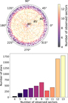 |
Fig. 1 Position of the investigated stars around the northern ecliptic pole in the ecliptic coordinates (top panel). The colour coding shows the number of sectors in which the data were available in the SPOC routine. The bottom panel shows in how many sectors the data were available for how many stars. |
2.2 Spectroscopic supporting data
To help to better classify the stars, we gathered available low-resolution spectra of 126 of our targets from the Large Sky Area Multi-Object Fiber Spectroscopic Telescope (LAMOST; R = λ/∆λ ≈ 1800, spectral range 3700–9000 Å) of the Chinese Academy of Science (Cui et al. 2012; Zhao et al. 2012) and determined their spectral type by using the MKCLASS code (Gray & Corbally 2014). This software is able to recover the spectral type with results that are comparable to the manual classification (e.g. Gray & Corbally 2014).
We also gathered new high-resolution spectra (R = λ/∆λ ≈ 40000 at Hα, spectral range 3800–9100 Å) to prove the rotational variability via projected rotational velocity of six stars that may be classified as pulsating stars. The stars were observed with the Ondřejov Echelle Spectrograph (OES) mounted on the 2 m Perek Telescope, Academy of Sciences, Czech Republic (Kabáth et al. 2020). All the spectra had signal-to-noise ratio (S/N) above 100 near Hα.
The spectra were modelled with the ISpec software (Blanco-Cuaresma et al. 2014; Blanco-Cuaresma 2019). As the input parameters for the fitting with radial transfer code SPECTRUM (Gray & Corbally 1994) and MARCS model atmosphere (Gustafsson et al. 2008), we used the values of Teff and log g from the TIC catalogue (Stassun et al. 2019) and adjusted them to better fit the spectra if necessary. Subsequently, we fixed these values and left ν sin i as a free parameter and determined the projected rotational velocity.
3 Identification of variability and data shortcomings
Stellar variability in the space data is usually investigated in the time (light curve) and frequency domains via Fourier transform (FT) of the data (e.g. Balona 2011; Bradley et al. 2015). We created the FT of the LC and SC SPOC and QLP data3 by using a Python implementation of the non-uniform fast FT4 that is significantly faster than a classical Lomb-Scargle periodogram (Lomb 1976; Scargle 1982) but gives basically the same results for TESS data.
The periodic signal with frequency ƒ in the data is usually considered as real if the S/N of the corresponding peak in the frequency spectrum is larger than four (Breger et al. 1993). However, higher S/N might be needed in case of stars with dense Fourier peaks (Bognár et al. 2020). We define the S/N as the ratio of the amplitude of the peak at a given frequency ƒ and the mean amplitude of the peaks in the vicinity of the peak f ± 1 c/d. This is a more conservative approach than using power-amplitude spectra or defining the S/N as the ratio of the amplitude of the peak and the standard deviation of the peaks in the immediate vicinity, as is often done (e.g. Balona 2011; De Medeiros et al. 2013). We did not apply any amplitude threshold (as was done e.g. by Uytterhoeven et al. 2011b; Bradley et al. 2015) because each target has a different noise level.
The basic problem in the identification (and classification of the variability in general) arises from the natural characteristics of the data (noise, sampling, time span of the data, data reduction and detrending) in combination with the variability timescales and amplitudes. We illustrate these issues in Figs. 2–3. The data reduced with different routines and with different sampling must naturally be different. As is apparent from the top panel of Fig. 2, the amplitude of the light variations in the LC data have smaller amplitudes averaging out the fast variations.
The QLP routine removes the large-amplitude variations by applying a high-pass filter (the bottom panel of Fig. 2, orange points, Huang et al. 2020a). From the bottom panel of Fig. 2, it is also apparent that residual instrumental and reduction artefacts due to imperfect background subtraction and/or poorly defined aperture might be present in the data (magenta diamonds, SPOC LC data). These artefacts appear more often in the SPOC LC data than in the SPOC SC or QLP data and can cause serious issues when classifying variability types. In the worst case, the artefacts can lead to a completely wrong classification. The QLP routine can even fully remove the variations (Fig. 2, bottom panel). A nice comparison of the available data products and their suitability for the large-amplitude variables investigation, particularly for Cepheids and RR Lyrae stars, observed by the Kepler (Borucki et al. 2010) and TESS missions, can be found in Plachy et al. (2019) and Molnár et al. (2022), respectively.
Figure 3 shows an example of how the frequency spectra for the SPOC data with different sampling can differ. There is a significant peak with S/N > 4 in the SC data (black line and points), while there is no significant peak in the FT of the LC data (yellow line and points). According to the SC data and the peak, TIC 2116199 should be considered as a variable star. However, because the FT of LC data shows no significant peak and there is actually no apparent variability in the light curve, we assume that the possible variation is of artificial nature and classify TIC 2116199 as a non-variable star.
From all the above mentioned reasons, we performed careful individual investigation of all available datasets for each star giving the preference to the SPOC SC data (where available) that seem to be the most reliable. The identification of variability and subsequent classification was performed on an individual basis. In addition, in case of LC data, the cadence is a significant fraction of the DSCT period and longer than that of a roAp star. Further shortcomings of the classification are discussed in Sect. 5.
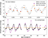 |
Fig. 2 Comparison of the data with different samplings obtained using different routines. In low-amplitude short-period variable stars, the LC data from QLP and SPOC data products give similar results but with smaller amplitudes (the upper panel). The bottom panel shows that in stars with amplitudes of the order of tens of millimagnitudes, the LC data can already suffer from some instrumental variations (magenta points), but the QLP routine (orange points) fully removes the variability. In both stars, the LC data are less reliable than the SC data in determining the amplitudes of brightness variations and in determining the variability type. |
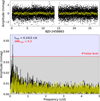 |
Fig. 3 SPOC data of TIC 2116199 from sector 14 (top panel) and frequency spectra based on four available sectors with a time span of 352 days (bottom panel). The LC data and the corresponding frequency spectrum are shown with yellow, and the SC data and the corresponding frequency spectrum with black. The horizontal dashed red line shows four times the noise level limit, while the vertical dotted blue line shows the most significant frequency |
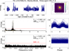 |
Fig. 4 Example of the figures that have been produced and used for the basic classification of each of the stars in the sample. The upper left panel shows the data, the top right panel shows the TPF with the aperture, and the middle and bottom panels show the frequency spectra (left) and the data phase-folded with the most prominent peaks in the frequency spectra (right). |
4 Classification scheme and notation
Similar to the identification of real variations (see Figs. 2–3), classification based solely on the photometric data can be a difficult task, leading to an ambiguous solutions. Usually, multi-parametric classification employing periods, light curves, and frequency spectra characteristics are used (e.g. Uytterhoeven et al. 2011b; Balona et al. 2011; Bradley et al. 2015). Some types of variable stars are recognizable upon a first look (typically the high-amplitude variables, for instance, eclipsing binaries of Algol type), but in some variability types the classification may even be impossible. For example, the light curve of an ellipsoidal variable can look the same (including periods and amplitudes) as an over-contact eclipsing variable of W UMa type, pulsating RRC star, or spotted chemically peculiar star; pulsations can mimic rotation, eclipses, and so on. (see Sect. 5).
For each star, we produced a figure showing the time series data, data phase-folded with the dominant frequencies below and above 5 c/d, a TPF with the aperture, and frequency spectra divided into parts below and above 5 c/d (Fig. 4). This frequency limit is a usually accepted value dividing the GDOR and DSCT pulsations (Grigahcène et al. 2010) that has been applied in many studies dealing with the data obtained from space (e.g. Uytterhoeven et al. 2011b; Balona et al. 2011; Bradley et al. 2015). Plots shown in Fig. 4 served as the main decision factors for the classification. If needed, particular stars were investigated more closely.
The basic variability types were adopted from the Variable Stars Index (VSX) catalogue5 (Watson et al. 2006). The notation is based on the classification system by the General Catalogue of Variable Stars (GCVS; Samus et al. 2009). For the stars that are certainly variable but we were not able to determine the variability type, we used “VAR”. If there is ambiguity between two or more variability types, we use the pipe symbol “|” meaning “or”. If a star shows a combination of variability types, we give plus sign with the variability type of larger amplitude listed first.
Because the temperature of the stars in our sample covers a wide range, the expected mixture of physical mechanisms of variability are also very broad. Thus, we examined the general characteristics of the light variations and put an emphasis on explaining the physical mechanism of the variability.
We considered finer divisions to more specific types only in high-amplitude stars (for example, EA versus EB, RRAB versus RRC, etc.). There were attempts to perform a more delicate classification also in low-amplitude classes of variables. For example, Balona et al. (2011) introduced three subclasses of GDOR stars according to their light-curve shape: symmetric (SYM), asymmetric (ASYM), and multiple modes (MULT). Similarly, Balona (2011) introduced three classes of rotationally variable stars: SPOT (multi-periodic with dominant frequency), SPOTM (clear travelling wave), and SPOTV (clear dominant period). Similar notation as for GDOR stars created by Balona et al. (2011) was introduced also for DSCT stars by Bradley et al. (2015). However, we did not perform such a detailed classification. The reasons are that there can be ambiguity in the variability types. Instead, we decided to build a classification on the assumed physical mechanisms rather than on the look of the light curve (see Sects. 4–5). We also did not distinguish between DSCT and SX Phe stars and do not divide DSCT into LADS and HADS classes (Frolov & Irkaev 1984; Petersen & Christensen-Dalsgaard 1996). Similarly, we do not distinguish between low-and high-amplitude GDOR stars (Paunzen et al. 2020).
The variability types and criteria for classification are listed in Tables 2–4 including light curves and corresponding frequency spectra of the typical examples. The types and results are explored in details in Sects. 5–6. In Sect. 5, we discuss details and problems in classification. In Tables 2–4, we do not show the minor variability types identified in our sample. We identified two RRAB/BL stars (RR Lyrae of AB type showing the Blazhko effect)6 and one RRC star7 accompanied with one RRAB and two RRC candidates that have amplitudes only in the mmag range, which is very suspicious. These two RRC candidates may belong to a new class of horizontal-branch variables (Wallace et al. 2019). We also found five candidates of roAp stars that show frequencies above 100 c/d.
In Table 5, we provide the identification, classification, frequency of the dominant peak in the FT and the amplitude of the brightness variation. We also give a cross-match of our sample with the VSX catalogue with the distance limit of 20”. There are 172 variable stars from our sample in the VSX (version 2022-02-21), while in 10 of the VSX stars we did not find any variation. For eclipsing binaries, we also give the zero epoch M0 of the primary eclipse in Table 5.
The amplitude given in Table 5 is a rough visual estimate of the maximum amplitude (from minimum to maximum light) seen in the data. For example, the amplitude of TIC 272749171 shown in Fig. 4 is 70mmag. This value is only indicative and can be different from the real amplitude of the variations. For example, the data might not contain the extrema of the variations, the light of the object can be contaminated by the light of nearby stars, the amplitude may be decreased by the LC in case of fast variations.
5 Ambiguity in classification and other related shortcomings
5.1 Blending
One of the reasons why we give only a rough estimate of the amplitude in Table 5 is that the value can be significantly affected by stars contaminating the light in the apertures (TESS has a spatial resolution of only 21″ px−1, Ricker et al. 2015). In an extreme case, the star in the sample itself can be stable and the variation can come from a nearby variable star. We did not investigate this issue in detail but we performed a quick analysis concerning stars within our sample. We checked stars that were closer than 10 pixels from each other. Based on the amplitude of the peaks in the frequency spectrum, we decided which star is variable and which is not.
Figure 5 shows two examples of blended stars. In the top panel, we can see that the variability comes from the fainter star, TIC 232681382, which has peaks in the FT with higher amplitudes. In the bottom panel, the situation is the opposite: the brighter star (TIC 233545407) is the variable. In our sample, we identified 29 such couples among stars classified as variable from which 21 pairs show the same FT with different amplitudes. For these cases, we comment in the last column of Table 5 that the variability is caused by a close companion.
There might be more blends with fainter stars, but a detailed inspection of the stars around each object in our sample is beyond the scope of this paper. Nevertheless, we cross-matched our sample with the Gaia DR2 catalogue (Gaia Collaboration 2018) and identified all stars that are less than 5 mag fainter (in Gaia g filter) than our variable star and are closer than 105″ (5 px) to it. We give the number of such stars in the last column of Table 5. This value gives at least a warning about possible blends that can also cause false positive identifications of variable stars.
5.2 Instrumental, data reduction artefacts, and semi-regular and long-period variations
The data we used is the SAP processed with the PDC pipeline (Smith et al. 2012; Stumpe et al. 2014). This pipeline uses co-trending basis vectors to remove systematics such as those resulting from the focus changes, spacecraft pointing jitter, and other stochastic errors, as well as the crowding problems (see e.g. Jenkins et al. 2016; Jenkins & et al. 2020; Kinemuchi et al. 2012). Mostly because of scattered light and due to improper aperture definition, there might be additional light variations present in the data (as already pointed out in Sect. 3) that is not intrinsic to the star. It is not always possible to distinguish between stellar variation and instrumental and reduction artefacts.
Generally, we expect that the instrumental/reduction artefacts will cause irregular or semi-regular variations with periods longer than 1 day producing groups of low-amplitude peaks with frequencies below 1 c/d in the FT. Typically, artefacts can be confused with stellar activity, rotational modulation due to spots, or GDOR type pulsations. From the high risk of instrumental artefacts or misclassification, we conservatively assigned spurious cases with a “VAR” label although some of the stars could be assigned with a particular variability class. Actually, stars showing similar light curves and FTs as TIC 334678134 and TIC 417734885 (shown in the top row of Table 3) have been often considered as stars showing rotational modulation or stellar activity (e.g. Balona 2011, 2013; Bradley et al. 2015).
Typical examples of the variability types caused by the binarity of the stars.
Typical examples of the variability types assumed to be caused by stellar pulsations.
5.3 Pulsating variable stars
There are three types of pulsators in the region of A-F stars near the main sequence. First of them are DSCT stars (p–mode pulsators) that are easily recognizable and the class is well defined because basically any variability with frequencies above 5 c/d is caused by pulsations of DSCT type (for examples see the figures in Table 3). There are also Population II stars that show similar behaviour as DSCT stars (SX Phe stars). However, we do not distinguish between these two types.
Regarding the FT, the upper limit of 100 c/d differentiates DSCTs from the second pulsating type, roAp stars (Kurtz 1982). However, the upper limit is not firmly set and depends on the particular author. The mechanism responsible for the rapid oscillations is not yet known. Currently the most accepted is the opacity mechanism in the hydrogen ionisation layer where the convection is suppressed by the magnetic field (Balmforth et al. 2001). Recently, Balona (2022) found that high frequencies appear also in non-magnetic stars, while DSCT frequencies were found in magnetic stars where they should be damped (Saio 2005; Murphy et al. 2020). Balona (2022) also found that there is no frequency limit differentiating DSCT from roAp frequencies and argues that there is no need for the roAp class.
The last type of pulsations occurring among A-F type main sequence stars are pulsations of GDOR type. The g-mode pulsations are believed to be excited by the convective flux blocking mechanism (Guzik et al. 2000; Dupret et al. 2005). Frequencies observed in GDOR pulsators are usually between 0.3 and 3 c/d (Kaye et al. 1999; Henry et al. 2011), but can also be above 5 c/d, although with small amplitudes (Grigahcène et al. 2010). Similarly, the DSCT pulsations can have frequencies below 5 c/d but with small amplitudes (Grigahcène et al. 2010). This can lead to a misclassification between GDOR and DSCT stars in a small fraction of stars. We classified a star as a GDOR if it shows two or more peaks with frequencies below 5 c/d that are not harmonics of each other. Peaks in the FT of GDOR stars often appear in groups (Balona et al. 2011; Saio et al. 2018). Such a pattern is characteristic for a significant portion of GDOR stars (see the examples in Table 3 and Fig. A.1). We cannot exclude the possibility that in clear GDOR stars some of the peaks can be caused by spots and rotation.
A significant fraction of the A-F pulsators show both GDOR and DSCT pulsations (see the examples in Table 3 and in Fig. A.2). Some of them were known prior to space missions (e.g. Henry & Fekel 2005; Handler 2009). These stars are called hybrids. Balona (2014) found that basically all DSCT stars show low-frequency peaks and are, therefore, hybrids, although some exceptions do exist (Bowman 2017). We marked a star as a hybrid when at least two significant peaks (S/N > 4) with frequencies below and above 5 c/d are present. This is a somewhat weaker criterion than has been used, for example, by Uytterhoeven et al. (2011b) and Bradley et al. (2015) who used an amplitude threshold and required that the amplitudes of the peaks in GDOR and DSCT regimes are similar (factor of 5–7). There is a risk that some of the frequencies can actually be a combination of other frequencies (Balona 2014; Bowman & Kurtz 2018). This could lead to a wrong hybrid classification. Further, in rapidly rotating GDOR stars, some of the peaks above 5 c/d can actually be g modes shifted to higher frequencies due to rotation (Bouabid et al. 2013). However, we assume that these issues would be present only in a small fraction of the stars. Because a detailed individual frequency analysis of the data is beyond the scope of this paper, we have not considered these effects in our classification.
A more serious problem for the classification and identification of the real highest peak in the FT is the presence of sub-Nyquist artefacts. In case of perfectly sampled data with a 30-min cadence, the value of the Nyquist frequency would be fNyquist = 24 c/d. Frequencies of some of the pulsation modes of DSCT stars can lie above this limit. A frequency ƒReal in range of 24 < ƒReal < 48 c/d will be reflected to a position fReflected = 2ƒnyquist – ƒReal = 48 – ƒReal. DSCT frequencies close to 2ƒNyquist will be reflected to a low-frequency region, where they possibly could mimic GDOR and ROTS frequencies. However, such frequencies will be heavily damped in amplitude, since the corresponding period of the pulsation cycle is comparable to the exposure time of the LC data (Balona 2014). We performed a simple test and compared the FT of LC and SC data and found out that about half of the GDOR candidates show a peak with higher amplitude close to 2ƒNyquist than close to 0 c/d in the LC data. However, the SC data showed in all cases that the frequencies below 5 c/d are the real ones and that there is no considerable risk that the GDOR stars are confused with DSCT stars due to Nyquist reflections.
Concerning the DSCT stars, the SC data ensure that the DSCT frequencies are identified properly and the classification is correct. In the LC data, the perfect sampling is disrupted by the downlink of the data, which causes the observations to not restart after exactly n×30 min (where n is an integer). This de-phasing is boosted in the TES S CVZ by multiple gaps (downlinks) and should allow for a reliable identification of the real pulsation frequencies of DSCT stars even if they are higher than fNyquist (Murphy 2015). However, the identification is not always perfect.
For stars classified as DSCT based on the LC data, we performed the FT analysis again in the range 0–60 c/d to retrieve possible frequencies above 24 c/d. To check how reliable these frequencies are in the LC data, we compared the results of 16% of all DSCT that have both LC and SC data (examples are shown in Fig. 6). The frequency with the highest amplitude identified in the SC data was successfully retrieved in only 50% of the test cases in the LC data (see panel D in Fig. 6). Thus, the DSCT frequencies above 24 c/d in Table 5 may be wrong in 50% of stars that do not have SC data. However, the classification as DSCT remains correct. Furthermore, we noticed that the frequency with the highest amplitude in the FT of SC data (that we expect to be the real dominant frequency) might not necessarily be the dominant frequency in the FT of LC data (panels A–C in Fig. 6). This is probably the result of the different sampling behaviour and smaller amplitude of the fast light variations in LC data.
Typical examples of the variability types caused by the rotation of a single star.
Sample of our classification table.
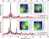 |
Fig. 5 Frequency spectra of two couples of blending stars. The apertures are shown in the insets. The red spectra correspond to non-variable stars contaminated by the nearby variables. The amplitudes of the peaks of non-variable blends are multiplied for a better visibility, by 10 and 40. |
5.4 Rotationally variable stars
Rotation is a stable phenomenon. Thus, in rotating stars, we expect regular pattern in form of harmonics (k f0) of the basic rotation frequency (ƒ0). The rotational variability can be induced by orbital motion of tidally deformed components of a non-eclipsing stars (ELL type, the last row in Table 2) or by spots on the surface of a single rotating star (Table 4). Among A-F type stars, these spots are believed to form via gravitational settling of light elements (He) and radiative lévitation of heavy and earth-rare elements (e.g. Si, Sr, Cr, and Eu) forming a class of chemically peculiar stars (Michaud 1970; Preston 1974). If a strong dipole magnetic field (inclined with respect to the rotational axis) is present, the spots formed usually around the magnetic poles can produce a rotational variability (Stibbs 1950; Kochukhov 2011).
The rotation periods of spotted stars are long – mostly of the order of days (Sikora et al. 2019) to hundreds of days or even years (Mathys 2017; Mathys et al. 2020). With 1-yr-long time base (at best), we are confined maximally to tens-of-days-long periods. The light curves of magnetic chemically peculiar stars have mostly sinusoidal or doubly sinusoidal light curves (Jagelka et al. 2019). We assign stars with stable light curves showing two (or more) harmonics in the FT as “ROTM” (meaning magnetic rotators, figures in the top row of Table 4) since we assume that the variation is caused by stable chemical spots that require strong magnetic fields8. Possible additional long-term variations are interpreted as instrumental/reduction artefacts (see Fig. 2). We do not assign sinusoidal variation (one significant peak in FT) as ROTM since it cannot be unambiguously distinguished from ELL type, and we classify these stars as ROTM|ELL (see Sect. 5.5).
As shown by many authors (e.g. Balona 2011, 2013; Hümmerich et al. 2018; Sikora et al. 2019), A-F stars can also show more complex light curves including amplitude variations. The variation can be highly irregular and can cause variations from cycle to cycle (see figures in the second row of Table 4 and also figures in e.g. Balona 2013; De Medeiros et al. 2013; Sikora et al. 2019; Trust et al. 2020). These variations are usually attributed to rotation and activity of a star with spots that can form and disappear and migrate due to differential rotation (solar-like activity; e.g. Balona 2011; Debosscher et al. 2011). However, one should be aware that mixing artefacts with real variations (see Fig. 2) can mimic time-varying spots.
Sikora et al. (2020) studied projected rotational velocities of 44 A- and late Β-type stars showing rotational modulation in their light curves and found out that more than 10%, but likely fewer than 30% of main sequence A-type stars show this type of variability. This is surprising, since stellar activity of this type is not expected in hot stars without large convective envelopes. We assign stars showing semi-regular variations producing groups of (un)resolved peaks at positions of harmonics in the FT as ROTS – rotators of solar type (figures in the second row of Table 4 and Fig. A.3). The groups of peaks are assumed to be the result of differential rotation.
Usually, authors assume that also semi-regular variations with small amplitude and variations producing one group of peaks (or a single peak) are signs of rotation or activity (e.g. Balona 2011; Uytterhoeven et al. 2011b; Bradley et al. 2015). We are more conservative and define such stars as VAR (see also Sect. 5.2).
Because there are many stars that show regular periodic patterns in the light curve that transforms into harmonics in the FT, we define the last type of rotational variability that is labelled as ROT (the last row in Table 4, Fig. A.3). The nature of these variations is, however, unclear. The origin can be explained by stable spots or some co-rotating structures governed by high-order magnetic multipoles, as suggested by Mikulášek et al. (2020) and Krtička et al. (2022) for the hot, chemically peculiar stars. However, more likely, these stars are a subgroup of GDOR stars (see Sect. 6).
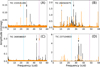 |
Fig. 6 Comparison of the FT based on the LC (orange) and SC (black) data for four DSCT stars. Frequencies with the highest amplitudes in the LC and SC data are marked with arrows of corresponding colour. The Nyquist frequency and its harmonic at 2ƒNyquist are shown with the vertical light blue and magenta lines, respectively. Panel A shows the example when the Nyquist reflection of the highest peak would be detected in LC data, panel Β shows the situation when the peak with the second highest amplitude would be the highest in the LC data, and panel C illustrates a situation when almost no variation is seen in the LC data and the identification completely failed in LC data. Panel D shows an example of when the proper peak would also be identified in LC data. |
5.5 Spotted stars or non-eclipsing binaries?
Without spectroscopic observations, based purely on single-passband photometry, there might be ambiguity between ROTM and ELL classes. In principle, the light variation of a spotted star (the top right-hand panel and red crosses in the middle panel of Fig. 7) can be equally described assuming gravity darkening caused by the tidal deformation of the components of a non-eclipsing system (the top left-hand panel and continuous line in the middle panel of Fig. 7). In addition, the amplitudes of the variations can be similar, as well as the periods and the FT.
Due to geometric reasons, ELL stars must reach the same brightness in maximum light twice a period. However, the same variation can be reproduced assuming two spots with different sizes on the opposite sides of a star (middle panel of Fig. 7). Thus, this is not a decisive criterion for ELLs. On the other hand, different maximum light typical to ROTM stars can be easily modelled assuming one spot on one of the components of a non-eclipsing binary system. Thus, again, different height of maxima should not be taken as the decisive criterion between ROTM and ELL types but only as a hint. In addition, there can be artefacts that cause a deformation in the light curve, making the correct classification more difficult (Fig. 2).
The ambiguity between ELL and ROTM can be demonstrated with a known ELL star IP Dra (the bottom panel of Fig. 7) that was spectroscopically confirmed to be a binary system (Kjurkchieva & Marchev 2014). The case of IP Dra shows the need of spectroscopic observations for reliable classification.
It was shown by Morris (1985) and Beech (1985) that if the light curve of ELL variables is described by the sum of sine and cosine functions  , Θ being phase, Ai and Bi amplitudes, A0 zero term), the term with the highest amplitude is cos(2Θ). This criterion is sometimes used as a support for the assumption of the ellipsoidal variability (e.g. Dal & Sipahi 2013; Li & Liu 2021). The light curve shown in Fig. 7 also shows dominant cos(2Θ). Since the dependence can be explained also with spots, the criterion with dominant cos(2Θ) is not sufficient for classifying the star as ELL.
Stable chemical spots and rotational modulation are usually observed in hot stars and only exceptionally occur among stars with Teff < 7000 Κ (Renson & Manfroid 2009; Hümmerich et al. 2018). In addition, the amplitude of the brightness variations usually decreases towards longer wavelengths (e.g. Krtička et al. 2007, 2015; Prvák et al. 2015). Therefore, we expect only negligible incidence rate of ROTM type among stars with temperatures below 7000 Κ and assign variations similar to those shown in Table 2 and Fig. 7 as ELL. Stars hotter than 7000 Κ showing rotational modulation with constant maximum brightness we assign as ROTM|ELL because of the ambiguity between these two types.
Faigler et al. (2012) found seven binary stars that show light curves typical to ROTM stars and confirmed them spectroscopically. They explain the shape of the light curves as a combination of reflection effects, ellipticity and Doppler boosting (Faigler & Mazeh 2011). Thus, it can easily happen that some of the stars classified as ROTM can actually be ELL. This example shows the unavoidable necessity of the spectroscopic observations in all ELL and ROTM stars to be properly classified.
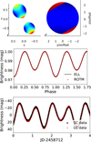 |
Fig. 7 Generated light curve (middle panel) assuming a non-eclipsing binary star with tidally deformed components (ELL, top left panel, black line in the middle panel) and a spotted star (ROTM, top right-hand panel, red crosses in the middle panel). An example of the light curve of a spectroscopically confirmed ELL star, IP Dra, that would rather be classified as ROTM is shown in the bottom panel. The models were generated using ELISa (Čokina et al. 2021). |
5.6 Pulsations or rotation?
To our best knowledge, there are no definitive criteria how to distinguish between rotation and pulsations based purely on photometric data. The issue with discriminating between pulsations and rotation was already pointed out by many studies, such as De Medeiros et al. (2013), who claimed that a better selection of rotating variables can only be made using spectroscopic observations. Balona et al. (2011) pointed out that irregular light curves can be attributed to slowly rotating stars and that the frequencies of the GDOR stars showing symmetric light curves or obvious beating are comparable to rotation frequencies. Actually, most of the studies dealing with the stellar classification based on the space data warn about the possible misclassification between pulsating stars and stars showing rotational variability (e.g. Uytterhoeven et al. 2011b; Balona 2011).
The typical rotational frequencies calculated from the median projected rotational velocity ν sin i and median radius R for A-F stars are between 0.5 and 0.75 c/d (Royer et al. 2007). However, the rotation frequencies can be as high as the critical rotational velocity, which corresponds to about 3–3.7 c/d in the fastest main sequence A-type stars (Sikora et al. 2019). Thus, there is a strong overlap of rotational variability and pulsations in the FT.
We performed a very simple test inspired by Sikora et al. (2020). We selected six bright examples of ROT, ROTS and GDOR stars and gathered spectra with the OES echelle spectrograph mounted at the Perek 2m telescope in Ondřejov, Czech Republic (see Sect. 2.2). We modelled the spectra using ISpec and measured the ν sin i (see Sect. 2.2). We calculated the bottom limit of the rotational frequency (v sin i ≤ vequatorial) by employing radii of the stars from the TIC catalogue (Stassun et al. 2019). The results are shown in Fig. 8.
Apparently, the measured frequencies agree well with the frequencies detected in the FT of the photometric data of the ROTS stars, while for GDOR and ROT stars the frequencies do not match well. However, the calculated frequencies shown with vertical dashed lines in Fig. 8 are only lower limits. It is possible that some of the peaks shown in the left panels of Fig. 8 can be addressed with inclined rotation axis and rotation. Thus, this test alone is not a proof that the variation in stars producing (un)resolved peaks at their harmonic positions in the FT are caused by rotation rather than pulsations. It is only strong support for this explanation. In addition, rotation of a star can shift the pulsation frequencies. An example how difficult the correct classification of such stars can be was published by Uytterhoeven et al. (2011a). They found that variations in HD 171834, which produce unresolved peaks at the harmonic positions in the FT, are caused by rotation rather than pulsations.
It is likely that there remain spurious cases in our sample that would need detailed investigation including spectroscopic observations. TIC 237218644 (top left panel of Fig. 9) would be classified as ROTS according to our methodology, but the temperature of 9087 ± 204 Κ (Stassun et al. 2019) suggests that the origin of the variations is probably pulsations rather than rotation, since at such high temperatures, stellar activity linked with convection is not expected. There might also be uncertainty in temperature. Due to all these issues, we classify TIC 237218644 as VAR. The remaining panels of Fig. 9 contain stars that show only one significant peak in the FT. These stars could possibly be classified as ROTS but also as GDOR, ELL or ROTM types. We conservatively classify such stars as VAR.
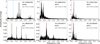 |
Fig. 8 Examples of FTs of GDOR (top left panel), ROT (bottom left panel), and ROTS stars (middle and right panels), showing also the position of frequencies calculated from observed ν sin i and catalogue radii of the stars (vertical colour lines). It is apparent that the calculated frequency corresponds well with the observed peaks in the FT of ROTS stars. |
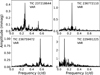 |
Fig. 9 Examples of frequency spectra of stars with ambiguous classification and, therefore, conservatively classified as VAR. See the text for details. |
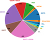 |
Fig. 10 Numbers of stars in particular variability classes. |
6 Results and discussion
We identified 3025 stars (out of 5923 in our sample, 51%) that show brightness variations. This is 12% less than reported on the basis of preliminary results (Skarka et al. 2021). From the 3025 stars, we were able to assign 1813 stars (60%) to a specific variability type. The number of stars in particular classes are shown in Fig. 10. The most numerous are GDOR and DSCT classes and their hybrids (together 64.9% of the variable stars). This is in excellent agreement with Uytterhoeven et al. (2011b) who found 63% of stars to show oscillations. Regarding eclipsing binaries (EA, EP, EAIEP, EB and EW classes), we found only 56% of our binary candidates in the TESS eclipsing binary catalogue9 (Prša et al. 2022). This discrepancy, however, comes from the fact that they used only 2-min cadence. If we use only the SC data, then the agreement of our identification with the TESS EB catalogue is 95%.
In the ‘Uncertain’ class, there are 34 stars with ambiguous classification with two equally probable types, for example ELL|ROTM and EA|EP. It was not possible to reliably classify the rest of the variable stars, marked as VAR (1212 stars; see Sect. 5). These are not shown in Fig. 10. In addition to the numbers given in Fig. 10, we identified 6 RR Lyrae stars (1 RRAB, 2 RRAB/BL, 3 RRC) and 7 heartbeat (HB) stars. In five stars we detected frequencies in the roAp range. However, it is not clear whether these are not combination frequencies. Not counting GDOR and DSCT hybrids, 50 stars show a combination of variability types, for example, EA+DSCT and GDOR+HB.
Plotting all the stars in the Hertzsprung–Russell diagram10 (HRD; Fig. 11) show some (expected) clumping. The vast majority of GDOR stars is located in a narrow part of the HRD well within the theoretical instability strip (IS) by (Dupret et al. 2005), as shown in the left panel of Fig. 11. The distribution of GDOR stars has maximum at around 7000 Κ and mean luminosity at about log L/L⊙ = 0.8 (Fig. 12). GDOR stars located outside the IS above approximately 7500 Κ are uniformly spread over the whole temperature range. Different behaviour of stars in and out of the IS suggests that the hot stars marked as GDOR outside of IS are not of the same type although the nature of the variability is likely to be g-mode pulsations.
The temperature distribution of DSCT and DSCT+GDOR hybrids is similar, although DSCT+GDOR hybrids are about 200 Κ hotter on average. GDOR+DSCT hybrids have preferentially lower temperatures than their DSCT-dominant counterparts but have the same average temperature as DSCT stars (see Fig. 12). There are a few GDOR, DSCT, and hybrid stars with unexpectedly low temperature. We checked them and would all of them classify as they are (see Fig. A.4). The unexpected behaviour at low temperatures might indicate contamination of the light by nearby stars or less reliable temperatures, although the error bars are similar to other stars in our sample. The groups of the rotating variables are well separated in the HRD. In addition, they have different temperature distributions. The ROTS stars (11.3%) dominate the low-temperature part of the HRD, which can be naturally expected as the variations are supposed to be caused by the spots of solar type. The ROTM stars (1.7%) are well spread out over the whole temperature range above 7000 K.
ROT stars (8.5%) are almost exclusively located near and within the cool edge of the GDOR instability strip. This suggests that the observed brightness variations are likely connected with pulsations rather than with rotation. Alternatively, rotation and pulsation can be present simultaneously and ROT stars could be a subclass of GDOR stars. The GDOR stars have an average temperature of 7043 Κ and a frequency of 1.358 c/d, while ROT stars have a mean temperature of 6777 Κ and a mean frequency of 0.578 c/d. The mean amplitude is significantly lower for ROT stars (1.5mmag) than for GDOR stars (9.8 mmag).
Our classification is in a very good agreement with the VSX classification. There are, of course, small differences but the variability types we provide are more specific or the same as in the VSX (with only a few exceptions). We applied our classification scheme to three of the previous studies dealing with the classification of variable stars based on the space data (Uytterhoeven et al. 2011b; Balona 2013; Bradley et al. 2015) to see the differences in the classification paying special attention to stars with frequencies below 5 c/d where the ambiguity between pulsation and rotation can emerge (see Sect 5.6). We downloaded the Kepler data of the stars with Lightkurve and performed the analysis exactly in the same way as for the stars in our sample.
Among 87 stars classified by Uytterhoeven et al. (2011b) as GDOR we found only 4 stars that we classified as ROTS and two stars that we classified as VAR. Thus, the agreement is excellent. However, in one third of stars classified by them as rotation or activity, we found that they are actually GDOR stars or hybrids (see examples in the four upper left-hand panels of Fig. 13). This is a significant discrepancy. In 25% of the stars classified as rotational variables by Balona (2013)11 we found GDOR variability (examples are shown in the four upper right-hand panels of Fig. 13) but we found perfect agreement for all 9 stars classified by Balona (2013) as GDOR.
The worst agreement with our classification is the classification by Bradley et al. (2015). From their sample of 195 GDOR stars we classified 9 as non-variable stars, 39 as VAR, 29 as ROTS, 6 as ROT, 2 as ROTM/ELL and one clear RR Lyrae (four bottom left panels of Fig. 13). This means that we classified 44% of stars marked by Bradley et al. (2015) as GDOR into a different variability class. We also checked 551 stars classified by Bradley et al. (2015) as rotating variables. We classified 403 of them (73%) as VAR or non-variables although the variability of the majority of these stars can be caused by the stellar activity (see the examples in four bottom right panels of Fig. 13). The rest of the stars in their sample we classified as ROTM, ROTS and ROT stars with only insignificant contamination of GDOR. In general, variability of a significant part of stars in the VAR class can be actually caused by stellar activity, but these variations usually have small amplitudes and the classification is not trustworthy. If we assume that all the stars from the sample of Bradley et al. (2015) classified by us as VAR are rotational variables, then the agreement with their study would be very good.
Misclassification can be a serious issue in statistical studies and in training procedures based on machine learning and neural network methods. All the issues and discrepancies described above show that a commonly accepted methodology and classification system is desirable but difficult to be built. The border cases with ambiguous classification will always be present. It is the reason why our classification is rather conservative. Theoretical limits for the frequencies of GDOR pulsations, would be very helpful to distinguish between rotation and pulsations in a significant part of stars. It is worth to mention that we have not noticed any flare in the light curves of the sample stars.
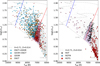 |
Fig. 11 Hertzsprung–Russell diagram showing pulsating stars (left panel) and rotationally modulated stars (right-hand panel). The dashed line shows the zero-age main sequence, dash-dotted lines show the evolutionary tracks for stars with different masses, all taken from Murphy et al. (2019). The blue and red continuous lines show the empirical boundaries of the instability strip determined by Murphy et al. (2019). The shaded area enclosed by the dotted lines shows the GDOR instability region, following Dupret et al. (2005). The grey dots show all stars including non-variable stars in our sample. |
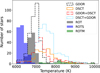 |
Fig. 12 Distribution of the stars with respect to their temperature. |
7 Conclusions and future prospects
We have performed a careful individual classification of 5923 A-F stars (temperatures between 6000 and 10 000 K) brighter than 11 mag located close by and in the northern TƁSS CVZ. The classification is based on the TESS photometric data and the properties of the frequency spectra. We discussed the data, crowding, the effects of residual variations caused by improper data reduction, aperture definition, and the influence of these effects on the classification of the variable stars. We have also discussed differences and similarities between the classes and paid special attention to a proper classification. We did not aim to study variability classes in detail, nor did we highlight any particular star. We also did not show any of the interesting cases. These remain for future dedicated studies.
We adopted the VSX classification scheme. We did not deal with the morphological classification of the variable stars within the variability classes, as was done by previous authors (e.g. Balona et al. 2011; Bradley et al. 2015). Our classification of the intrinsic variability is based on the assumption of the basic physical phenomena, that is, rotation and pulsations. We introduced three classes of rotationally modulated stars: stars with stable chemical spots (ROTM), stars with regular brightness variations (ROT), and stars showing semi-regular variations assumed to be caused by the forming or ceasing of the spots in combination with differential rotation (ROTS).
Our main results and findings can be summarised as follows:
The PDCSAP data with different cadences are generally different in both amplitude and cadence. Mainly the 30-min data suffer from lots of residual variability that is not coming from the stars. This can lead to false positives and wrong classifications;
We provide a well-defined classification scheme and methodology for the proper classification of A-F variable stars based on the light-curve shape and the corresponding FT (Tables 2–4);
We find that the identification of the real pulsation frequencies above the Nyquist limit based purely on the amplitudes of the corresponding peaks in the FT can be wrong in up to 50% of cases;
We identify a new (sub)class of variables that show regular periodic light-curve shapes and harmonics of the basic frequency in the FT. First we assumed that these variations must be connected with rotation, but the position of these stars close to and within the GDOR instability strip suggests that the variations are likely caused by pulsations. ROT stars have longer periods (1.7 versus 0.74 days), smaller amplitudes (1.5 versus 9.8 mmag), and are cooler on average (6777 versus 7043 K) than GDOR stars. The position of the stars in the HRD also suggests that the idea of co-rotating structures governed by high-order magnetic multipoles (Mikulášek et al. 2020; Krtička et al. 2022) likely cannot explain the variations in these relatively cool stars that are not expected to have strong stellar winds;
Measurements of v sin i of four stars that show semi-regular brightness variations and unresolved groups of peaks near the harmonics of the basic frequency give a hint that the observed light variations may be linked with rotation rather than with pulsations. Stars in this group, called ROTS, can be mostly easily recognised from the GDOR stars;
If the model of the light curve provides physically plausible results, there is no way to unambiguously distinguish between ellipsoidal variables and ROTM types purely on the basis of single-channel photometry. We have demonstrated this issue on IP Dra and generated models (Fig. 7).
On the comparison with previous studies, we have demonstrated that a commonly accepted classification scheme should be agreed upon. Our approach offers a well-defined system of classification with many examples. There still might be spurious cases, mainly regarding the GDOR, ROTS, and ROT classes; however, our sample should be clear of such ambiguous stars since we classified the spurious cases as VAR. The theoretical study of the limits of g-mode pulsations and all the possible patterns that can be expected in the FT would be very helpful in the future to better distinguish between rotation and pulsations. The only way to reliably classify the variable stars is via a detailed case-by-case investigation that includes spectroscopic data. We warn about any blind usage of the (mainly LC) TESS data.
The approach presented in the paper is rather conservative. Our groups of stars provide good and reliable samples of stars without significant contamination suitable for statistical studies and the training of neural networks. We are planning spectroscopic observations and detailed investigations of particularly interesting stars identified during the analysis of the data. We will perform the same analysis for the southern TESS CVZ.
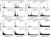 |
Fig. 13 Frequency spectra of stars observed by the Kepler mission and classified in previous studies (shown on the top of every four plots). The labels give how the stars would be classified using our methodology. |
Acknowledgements
M. S., P. K., and R. K. acknowledge the support by Inter-transfer grant no LTT-20015. M. M. acknowledges the support by MEYS (Czech Republic) under the project MEYS LTT17006. This paper includes data collected with the TESS mission. Funding for the TESS mission is provided by the NASA Explorer Program. Funding for the TESS Asteroseismic Science Operations Centre is provided by the Danish National Research Foundation (Grant agreement no.: DNRF106), ESA PRODEX (PEA 4000119301) and Stellar Astrophysics Centre (SAC) at Aarhus University. We thank the TESS team and staff and TASC/TASOC for their support of the present work. We also thank the TASC WG4 team for their contribution to the selection of targets for 2-min observations. The TESS data were obtained from the MAST data archive at the Space Telescope Science Institute (STScI). We acknowledge the usage of the data taken with the Perek telescope at the Astronomical Institute of the Czech Academy of Sciences in Ondřejov and would like to thank the observers for their work. We thank the referee for useful comments that improved the manuscript.
We used Teff from the TIC catalogue (Stassun et al. 2019).
In the range of 0–300 and 0–24 c/d for the SC and LC data, respectively.
Saw-tooth light-curve shape, harmonics of the basic frequency in FT.
More sinusoidal shape, harmonics of the basic frequency in FT.
Jagelka et al. (2019) show that the role of the magnetic field in forming the chemical spots may not be as important as is formerly supposed.
Temperatures are taken from Stassun et al. (2019), luminosity of the stars calculated from temperatures and radii from Stassun et al. (2019).
We checked only the first 200 stars from the list of Balona (2013).
Appendix A Examples of Typical Light Curves and Frequency Spectra
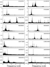 |
Fig. A.1 Typical frequency spectra of GDOR stars. The four bottom-most plots show less certain cases. Τhe scale on the vertical axis is in mmag. The labels show the TIC numbers. |
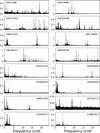 |
Fig. A.2 Typical frequency spectra of GDOR and DSCT Hybrid stars. The eight upper panels show DSCT dominant, while the eight bottom panels show the GDOR dominant hybrids. TIC 198188157 and 198389350 show weak peaks in the GDOR regime and, thus, are less certain hybrids. TIC 219105073 and 219867827 show only low-amplitude peaks in the DSCT regime and, thus, are less certain hybrids. The less certain hybrids can possibly be classified as pure GDOR or DSCT stars. The scale on the vertical axis is in mmag. |
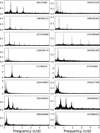 |
Fig. A.3 Typical frequency spectra of ROT (eight upper panels) and ROTS stars (eight bottom panels). The scale on the vertical axis is in mmag. |
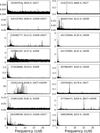 |
Fig. A.4 Frequency spectra of the coolest pulsating stars in our sample. The first number is the TIC number, trie second number gives the temperature from TIC catalogue. The scale on the vertical axis is in mmag. |
References
- Antoci, V., Cunha, M., Houdek, G., et al. 2014, ApJ, 796, 118 [Google Scholar]
- Antoci, V., Cunha, M.S., Bowman, D.M., et al. 2019, MNRAS, 490, 4040 [NASA ADS] [CrossRef] [Google Scholar]
- Audenaert, J., Kuszlewicz, J.S., Handberg, R., et al. 2021, AJ, 162, 209 [NASA ADS] [CrossRef] [Google Scholar]
- Balmforth, N.J., Cunha, M.S., Dolez, N., Gough, D.O., & Vauclair, S. 2001, MNRAS, 323, 362 [NASA ADS] [CrossRef] [Google Scholar]
- Balona, L.A. 2011, MNRAS, 415, 1691 [NASA ADS] [CrossRef] [Google Scholar]
- Balona, L.A. 2012, MNRAS, 423, 3420 [NASA ADS] [CrossRef] [Google Scholar]
- Balona, L.A. 2013, MNRAS, 431, 2240 [NASA ADS] [CrossRef] [Google Scholar]
- Balona, L.A. 2014, MNRAS, 437, 1476 [NASA ADS] [CrossRef] [Google Scholar]
- Balona, L.A. 2022, MNRAS, 510, 5743 [NASA ADS] [CrossRef] [Google Scholar]
- Balona, L.A., & Nemec, J.M. 2012, MNRAS, 426, 2413 [NASA ADS] [CrossRef] [Google Scholar]
- Balona, L.A., Krisciunas, K., & Cousins, A.W.J. 1994, MNRAS, 270, 905 [NASA ADS] [CrossRef] [Google Scholar]
- Balona, L.A., Guzik, J.A., Uytterhoeven, K., et al. 2011, MNRAS, 415, 3531 [NASA ADS] [CrossRef] [Google Scholar]
- Barentsen, G., & Lightkurve Collaboration. 2020, in American Astronomical Society Meeting Abstracts, 235, 409.04 [NASA ADS] [Google Scholar]
- Beech, M. 1985, Ap&SS, 117, 69 [Google Scholar]
- Blanco-Cuaresma, S. 2019, MNRAS, 486, 2075 [Google Scholar]
- Blanco-Cuaresma, S., Soubiran, C., Heiter, U., & Jofré, P. 2014, A&A, 569, A111 [CrossRef] [EDP Sciences] [Google Scholar]
- Boch, T., Pineau, F., & Derriere, S. 2012, in Astronomical Society of the Pacific Conference Series, Astronomical Data Analysis Software and Systems XXI, eds. P. Ballester, D. Egret, & N.P.F. Lorente, 461, 291 [NASA ADS] [Google Scholar]
- Bognár, Z., Kawaler, S.D., Bell, K.J., et al. 2020, A&A, 638, A82 [NASA ADS] [CrossRef] [EDP Sciences] [Google Scholar]
- Borucki, W.J., Koch, D., Basri, G., et al. 2010, Science, 327, 977 [Google Scholar]
- Bouabid, M.P., Dupret, M.A., Salmon, S., et al. 2013, MNRAS, 429, 2500 [NASA ADS] [CrossRef] [Google Scholar]
- Bowman, D.M. 2017, Amplitude Modulation of Pulsation Modes in Delta Scuti Stars (Springer International Publishing) [CrossRef] [Google Scholar]
- Bowman, D.M., & Kurtz, D.W. 2018, MNRAS, 476, 3169 [NASA ADS] [CrossRef] [Google Scholar]
- Bradley, P.A., Guzik, J.A., Miles, L.F., et al. 2015, AJ, 149, 68 [CrossRef] [Google Scholar]
- Breger, M. 2000, in Astronomical Society of the Pacific Conference Series, Delta Scuti and Related Stars, eds. M. Breger, & M. Montgomery, 210, 3 [NASA ADS] [Google Scholar]
- Breger, M., Stich, J., Garrido, R., et al. 1993, A&A, 271, 482 [NASA ADS] [Google Scholar]
- Catelan, M., & Smith, H.A. 2015, Pulsating Stars (Wiley-VCH) [CrossRef] [Google Scholar]
- Čokina, M., Fedurco, M., & Parimucha, Š. 2021, A&A, 652, A156 [NASA ADS] [CrossRef] [EDP Sciences] [Google Scholar]
- Cox, J.P. 1963, ApJ, 138, 487 [NASA ADS] [CrossRef] [Google Scholar]
- Cui, X.-Q., Zhao, Y.-H., Chu, Y.-Q., et al. 2012, Res. Astron. Astrophys., 12, 1197 [Google Scholar]
- Cunha, M.S., Antoci, V., Holdsworth, D.L., et al. 2019, MNRAS, 487, 3523 [NASA ADS] [CrossRef] [Google Scholar]
- Dal, H.A., & Sipahi, E. 2013, PASA, 30, e016 [NASA ADS] [CrossRef] [Google Scholar]
- De Medeiros, J.R., Ferreira Lopes, C.E., Leäo, I.C., et al. 2013, A&A, 555, A63 [NASA ADS] [CrossRef] [EDP Sciences] [Google Scholar]
- Debosscher, J., Blomme, J., Aerts, C., & De Ridder, J. 2011, A&A, 529, A89 [NASA ADS] [CrossRef] [EDP Sciences] [Google Scholar]
- Dupret, M.A., Grigahcène, A., Garrido, R., Gabriel, M., & Scuflaire, R. 2005, A&A, 435, 927 [NASA ADS] [CrossRef] [EDP Sciences] [Google Scholar]
- Faigler, S., & Mazeh, T. 2011, MNRAS, 415, 3921 [Google Scholar]
- Faigler, S., Mazeh, T., Quinn, S.N., Latham, D.W., & Tal-Or, L. 2012, ApJ, 746, 185 [NASA ADS] [CrossRef] [Google Scholar]
- Frolov, M.S., & Irkaev, B.N. 1984, Inform. Bull. Variable Stars, 2462, 1 [NASA ADS] [Google Scholar]
- Gaia Collaboration (Brown, A.G.A., et al.) 2018, A&A, 616, A1 [NASA ADS] [CrossRef] [EDP Sciences] [Google Scholar]
- Gray, R.O., & Corbally, C.J. 1994, AJ, 107, 742 [NASA ADS] [CrossRef] [Google Scholar]
- Gray, R.O., & Corbally, C.J. 2014, AJ, 147, 80 [CrossRef] [Google Scholar]
- Grigahcène, A., Antoci, V., Balona, L., et al. 2010, ApJ, 713, L192 [Google Scholar]
- Gustafsson, B., Edvardsson, B., Eriksson, K., et al. 2008, A&A, 486, 951 [NASA ADS] [CrossRef] [EDP Sciences] [Google Scholar]
- Guzik, J.A., Kaye, A.B., Bradley, P.A., Cox, A.N., & Neuforge, C. 2000, ApJ, 542, L57 [NASA ADS] [CrossRef] [Google Scholar]
- Handler, G. 2009, MNRAS, 398, 1339 [NASA ADS] [CrossRef] [Google Scholar]
- Henry, G.W., & Fekel, F.C. 2005, AJ, 129, 2026 [NASA ADS] [CrossRef] [Google Scholar]
- Henry, G.W., Fekel, F.C., & Henry, S.M. 2011, AJ, 142, 39 [NASA ADS] [CrossRef] [Google Scholar]
- Houdek, G. 2000, in Astronomical Society of the Pacific Conference Series, Delta Scuti and Related Stars, eds. M. Breger & M. Montgomery, 210, 454 [NASA ADS] [Google Scholar]
- Huang, C.X., Vanderburg, A., Pal, A., et al. 2020a, RNAAS, 4, 204 [NASA ADS] [Google Scholar]
- Huang, C.X., Vanderburg, A., Pal, A., et al. 2020b, RNAAS, 4, 206 [NASA ADS] [Google Scholar]
- Hümmerich, S., Mikulašek, Z., Paunzen, E., et al. 2018, A&A, 619, A98 [NASA ADS] [CrossRef] [EDP Sciences] [Google Scholar]
- Jagelka, M., Mikulašek, Z., Hümmerich, S., & Paunzen, E. 2019, A&A, 622, A199 [NASA ADS] [CrossRef] [EDP Sciences] [Google Scholar]
- Jenkins, J.M., Twicken, J.D., McCauliff, S., et al. 2016, SPIE Conf. Ser., 9913, 99133E [NASA ADS] [Google Scholar]
- Jenkins, J.M., et al. 2020, Kepler Science Document KSCI-19081-003 [Google Scholar]
- Kabáth, P., Skarka, M., Sabotta, S., et al. 2020, PASP, 132, 035002 [CrossRef] [Google Scholar]
- Kaye, A.B., Handler, G., Krisciunas, K., Poretti, E., & Zerbi, F.M. 1999, PASP, 111, 840 [NASA ADS] [CrossRef] [Google Scholar]
- Kinemuchi, K., Barclay, T., Fanelli, M., et al. 2012, PASP, 124, 963 [Google Scholar]
- Kjurkchieva, D., & Marchev, D. 2014, Inform. Bull. Variable Stars, 6096, 1 [NASA ADS] [Google Scholar]
- Kochukhov, O. 2011, in Physics of Sun and Star Spots, eds. D. Prasad Choudhary, & K.G. Strassmeier, 273, 249 [NASA ADS] [Google Scholar]
- KrtiCka, J., Mikulašek, Z., Zverko, J., & Žižnovsky, J. 2007, A&A, 470, 1089 [NASA ADS] [CrossRef] [EDP Sciences] [Google Scholar]
- KrtiCka, J., Mikulašek, Z., Lüftinger, T., & Jagelka, M. 2015, A&A, 576, A82 [NASA ADS] [CrossRef] [EDP Sciences] [Google Scholar]
- KrtiCka, J., Mikulašek, Z., Kurfürst, P., & Oksala, M.E. 2022, A&A, 659, A37 [NASA ADS] [CrossRef] [EDP Sciences] [Google Scholar]
- Kurtz, D.W. 1982, MNRAS, 200, 807 [NASA ADS] [CrossRef] [Google Scholar]
- Li, X.-Z., & Liu, L. 2021, New Astron., 84, 101539 [NASA ADS] [CrossRef] [Google Scholar]
- Lightkurve Collaboration, (Cardoso, J.V.D.M., et al.) 2018, Lightkurve: Kepler and TESS time series analysis in Python, AstrophysiCs SourCe Code Library [record ascl:1812.013] [Google Scholar]
- Lomb, N.R. 1976, Ap&SS, 39, 447 [NASA ADS] [CrossRef] [Google Scholar]
- Mathys, G. 2017, A&A, 601, A14 [NASA ADS] [CrossRef] [EDP Sciences] [Google Scholar]
- Mathys, G., Kurtz, D.W., & Holdsworth, D.L. 2020, A&A, 639, A31 [NASA ADS] [CrossRef] [EDP Sciences] [Google Scholar]
- MiChaud, G. 1970, ApJ, 160, 641 [NASA ADS] [CrossRef] [Google Scholar]
- Mikulašek, Z., KrtiCka, J., Shultz, M.E., et al. 2020, in Stellar Magnetism: A Workshop in Honour of the Career and Contributions of John D. Landstreet, eds. G. Wade, E. AleCian, D. Bohlender, & A. Sigut, 11, 46 [Google Scholar]
- Molnár, L., Bodi, A., Pal, A., et al. 2022, ApJS, 258, 8 [CrossRef] [Google Scholar]
- Morris, S.L. 1985, ApJ, 295, 143 [NASA ADS] [CrossRef] [Google Scholar]
- Murphy, S.J. 2015, MNRAS, 453, 2569 [NASA ADS] [Google Scholar]
- Murphy, S.J., Hey, D., Van Reeth, T., & Bedding, T.R. 2019, MNRAS, 485, 2380 [NASA ADS] [CrossRef] [Google Scholar]
- Murphy, S.J., Saio, H., Takada-Hidai, M., et al. 2020, MNRAS, 498, 4272 [NASA ADS] [CrossRef] [Google Scholar]
- Paunzen, E., Bernhard, K., Hümmerich, S., et al. 2020, MNRAS, 499, 3976 [NASA ADS] [CrossRef] [Google Scholar]
- Petersen, J.O., & Christensen-Dalsgaard, J. 1996, A&A, 312, 463 [NASA ADS] [Google Scholar]
- Pedersen, M.G., Antoci, V., Korhonen, H., et al. 2017, MNRAS, 466, 3060 [NASA ADS] [CrossRef] [Google Scholar]
- Pineau, F.-X., Boch, T., Derrière, S., & Schaaff, A. 2020, in Astronomical Society of the Pacific Conference Series, Astronomical Data Analysis Software and Systems XXVII, eds. P. Ballester, J. Ibsen, M. Solar, & K. Shortridge, 522, 125 [NASA ADS] [Google Scholar]
- Plachy, E., Molnar, L., Bodi, A., et al. 2019, ApJS, 244, 32 [CrossRef] [Google Scholar]
- Preston, G.W. 1974, ARA&A, 12, 257 [NASA ADS] [CrossRef] [Google Scholar]
- Prvák, M., Liška, J., Krticka, J., Mikulašek, Z., & Lüftinger, T. 2015, A&A, 584, A17 [NASA ADS] [CrossRef] [EDP Sciences] [Google Scholar]
- Prša, A., Kochoska, A., Conroy, K.E., et al. 2022, ApJS, 258, 16 [CrossRef] [Google Scholar]
- Renson, P., & Manfroid, J. 2009, A&A, 498, 961 [NASA ADS] [CrossRef] [EDP Sciences] [Google Scholar]
- Ricker, G.R., Winn, J.N., Vanderspek, R., et al. 2015, J. Astron. Telesc. Instrum. Syst., 1, 014003 [Google Scholar]
- Royer, F., Zorec, J., & Gomez, A.E. 2007, A&A, 463, 671 [NASA ADS] [CrossRef] [EDP Sciences] [Google Scholar]
- Saio, H. 2005, MNRAS, 360, 1022 [NASA ADS] [CrossRef] [Google Scholar]
- Saio, H., Bedding, T.R., Kurtz, D.W., et al. 2018, MNRAS, 477, 2183 [NASA ADS] [CrossRef] [Google Scholar]
- Samus, N.N., Kazarovets, E.V., Durlevich, O.V., Kireeva, N.N., & Pastukhova, E.N. 2009, VizieR Online Data Catalog: B/gcvs [Google Scholar]
- Sánchez Arias, J.P., Corsico, A.H., & Althaus, L.G. 2017, A&A, 597, A29 [NASA ADS] [CrossRef] [EDP Sciences] [Google Scholar]
- Scargle, J.D. 1982, ApJ, 263, 835 [NASA ADS] [CrossRef] [Google Scholar]
- Sikora, J., David-Uraz, A., Chowdhury, S., et al. 2019, MNRAS, 487, 4695 [Google Scholar]
- Sikora, J., Wade, G.A., & Rowe, J. 2020, MNRAS, 498, 2456 [NASA ADS] [CrossRef] [Google Scholar]
- Skarka, M., Auer, R.F., Henzl, Z., et al. 2021, in Posters from the TESS Science Conference II (TSC2), 31 [Google Scholar]
- Smith, J.C., Stumpe, M.C., Van Cleve, J.E., et al. 2012, PASP, 124, 1000 [NASA ADS] [CrossRef] [Google Scholar]
- Stassun, K.G., Oelkers, R.J., Paegert, M., et al. 2019, AJ, 158, 138 [NASA ADS] [CrossRef] [Google Scholar]
- Stibbs, D.W.N. 1950, MNRAS, 110, 395 [Google Scholar]
- Stumpe, M.C., Smith, J.C., Catanzarite, J.H., et al. 2014, PASP, 126, 100 [NASA ADS] [CrossRef] [Google Scholar]
- Trust, O., Jurua, E., De Cat, P., & Joshi, S. 2020, MNRAS, 492, 3143 [NASA ADS] [CrossRef] [Google Scholar]
- Twicken, J.D., Chandrasekaran, H., Jenkins, J.M., et al. 2010, SPIE Conf. Ser., 7740, 77401U [NASA ADS] [Google Scholar]
- Uytterhoeven, K., Mathias, P., Baglin, A., et al. 2011a, ArXiv e-prints [arXiv:1111.1840] [Google Scholar]
- Uytterhoeven, K., Moya, A., Grigahcène, A., et al. 2011b, A&A, 534, A125 [CrossRef] [EDP Sciences] [Google Scholar]
- Wallace, J.J., Hartman, J.D., Bakos, G.A., & Bhatti, W. 2019, ApJ, 870, L7 [NASA ADS] [CrossRef] [Google Scholar]
- Watson, C.L., Henden, A.A., & Price, A. 2006, 25th Annual Symposium, The Society for Astronomical Sciences, 47 [Google Scholar]
- Wenger, M., Ochsenbein, F., Egret, D., et al. 2000, A&As, 143, 9 [NASA ADS] [CrossRef] [EDP Sciences] [Google Scholar]
- Zhao, G., Zhao, Y.-H., Chu, Y.-Q., Jing, Y.-P., & Deng, L.-C. 2012, Res. Astron. Astrophys., 12, 723 [NASA ADS] [CrossRef] [Google Scholar]
All Tables
Distribution of the number of stars in particular temperature (top part) and brightness (bottom part) ranges of the sample stars (from the TIC; Stassun et al. 2019).
Typical examples of the variability types assumed to be caused by stellar pulsations.
Typical examples of the variability types caused by the rotation of a single star.
All Figures
|
Fig. 1 Position of the investigated stars around the northern ecliptic pole in the ecliptic coordinates (top panel). The colour coding shows the number of sectors in which the data were available in the SPOC routine. The bottom panel shows in how many sectors the data were available for how many stars. |
| In the text | |
|
Fig. 2 Comparison of the data with different samplings obtained using different routines. In low-amplitude short-period variable stars, the LC data from QLP and SPOC data products give similar results but with smaller amplitudes (the upper panel). The bottom panel shows that in stars with amplitudes of the order of tens of millimagnitudes, the LC data can already suffer from some instrumental variations (magenta points), but the QLP routine (orange points) fully removes the variability. In both stars, the LC data are less reliable than the SC data in determining the amplitudes of brightness variations and in determining the variability type. |
| In the text | |
|
Fig. 3 SPOC data of TIC 2116199 from sector 14 (top panel) and frequency spectra based on four available sectors with a time span of 352 days (bottom panel). The LC data and the corresponding frequency spectrum are shown with yellow, and the SC data and the corresponding frequency spectrum with black. The horizontal dashed red line shows four times the noise level limit, while the vertical dotted blue line shows the most significant frequency |
| In the text | |
|
Fig. 4 Example of the figures that have been produced and used for the basic classification of each of the stars in the sample. The upper left panel shows the data, the top right panel shows the TPF with the aperture, and the middle and bottom panels show the frequency spectra (left) and the data phase-folded with the most prominent peaks in the frequency spectra (right). |
| In the text | |
|
Fig. 5 Frequency spectra of two couples of blending stars. The apertures are shown in the insets. The red spectra correspond to non-variable stars contaminated by the nearby variables. The amplitudes of the peaks of non-variable blends are multiplied for a better visibility, by 10 and 40. |
| In the text | |
|
Fig. 6 Comparison of the FT based on the LC (orange) and SC (black) data for four DSCT stars. Frequencies with the highest amplitudes in the LC and SC data are marked with arrows of corresponding colour. The Nyquist frequency and its harmonic at 2ƒNyquist are shown with the vertical light blue and magenta lines, respectively. Panel A shows the example when the Nyquist reflection of the highest peak would be detected in LC data, panel Β shows the situation when the peak with the second highest amplitude would be the highest in the LC data, and panel C illustrates a situation when almost no variation is seen in the LC data and the identification completely failed in LC data. Panel D shows an example of when the proper peak would also be identified in LC data. |
| In the text | |
|
Fig. 7 Generated light curve (middle panel) assuming a non-eclipsing binary star with tidally deformed components (ELL, top left panel, black line in the middle panel) and a spotted star (ROTM, top right-hand panel, red crosses in the middle panel). An example of the light curve of a spectroscopically confirmed ELL star, IP Dra, that would rather be classified as ROTM is shown in the bottom panel. The models were generated using ELISa (Čokina et al. 2021). |
| In the text | |
|
Fig. 8 Examples of FTs of GDOR (top left panel), ROT (bottom left panel), and ROTS stars (middle and right panels), showing also the position of frequencies calculated from observed ν sin i and catalogue radii of the stars (vertical colour lines). It is apparent that the calculated frequency corresponds well with the observed peaks in the FT of ROTS stars. |
| In the text | |
|
Fig. 9 Examples of frequency spectra of stars with ambiguous classification and, therefore, conservatively classified as VAR. See the text for details. |
| In the text | |
|
Fig. 10 Numbers of stars in particular variability classes. |
| In the text | |
|
Fig. 11 Hertzsprung–Russell diagram showing pulsating stars (left panel) and rotationally modulated stars (right-hand panel). The dashed line shows the zero-age main sequence, dash-dotted lines show the evolutionary tracks for stars with different masses, all taken from Murphy et al. (2019). The blue and red continuous lines show the empirical boundaries of the instability strip determined by Murphy et al. (2019). The shaded area enclosed by the dotted lines shows the GDOR instability region, following Dupret et al. (2005). The grey dots show all stars including non-variable stars in our sample. |
| In the text | |
|
Fig. 12 Distribution of the stars with respect to their temperature. |
| In the text | |
|
Fig. 13 Frequency spectra of stars observed by the Kepler mission and classified in previous studies (shown on the top of every four plots). The labels give how the stars would be classified using our methodology. |
| In the text | |
|
Fig. A.1 Typical frequency spectra of GDOR stars. The four bottom-most plots show less certain cases. Τhe scale on the vertical axis is in mmag. The labels show the TIC numbers. |
| In the text | |
|
Fig. A.2 Typical frequency spectra of GDOR and DSCT Hybrid stars. The eight upper panels show DSCT dominant, while the eight bottom panels show the GDOR dominant hybrids. TIC 198188157 and 198389350 show weak peaks in the GDOR regime and, thus, are less certain hybrids. TIC 219105073 and 219867827 show only low-amplitude peaks in the DSCT regime and, thus, are less certain hybrids. The less certain hybrids can possibly be classified as pure GDOR or DSCT stars. The scale on the vertical axis is in mmag. |
| In the text | |
|
Fig. A.3 Typical frequency spectra of ROT (eight upper panels) and ROTS stars (eight bottom panels). The scale on the vertical axis is in mmag. |
| In the text | |
|
Fig. A.4 Frequency spectra of the coolest pulsating stars in our sample. The first number is the TIC number, trie second number gives the temperature from TIC catalogue. The scale on the vertical axis is in mmag. |
| In the text | |
Current usage metrics show cumulative count of Article Views (full-text article views including HTML views, PDF and ePub downloads, according to the available data) and Abstracts Views on Vision4Press platform.
Data correspond to usage on the plateform after 2015. The current usage metrics is available 48-96 hours after online publication and is updated daily on week days.
Initial download of the metrics may take a while.