| Issue |
A&A
Volume 688, August 2024
|
|
|---|---|---|
| Article Number | A25 | |
| Number of page(s) | 10 | |
| Section | Catalogs and data | |
| DOI | https://doi.org/10.1051/0004-6361/202450711 | |
| Published online | 30 July 2024 | |
Periodic variable A-F spectral type stars in the southern TESS continuous viewing zone
I. Identification and classification★
1
Astronomical Institute of the Czech Academy of Sciences,
Fričova 298,
25165
Ondřejov,
Czech Republic
e-mail: This email address is being protected from spambots. You need JavaScript enabled to view it.
2
Department of Theoretical Physics and Astrophysics, Masaryk University,
Kotlářská 2,
61137
Brno,
Czech Republic
3
Variable Star and Exoplanet Section of the Czech Astronomical Society,
Fričova 298,
251 65
Ondřejov,
Czech Republic
4
Hvězdárna Jaroslava Trnky ve Slaném,
Nosačická 1713, Slaný 1,
27401
Slaný,
Czech Republic
Received:
14
May
2024
Accepted:
15
June
2024
Abstract
Aims. Our primary objective is to accurately identify and classify the variability of A-F stars in the southern continuous viewing zone of the TESS satellite. The brightness limit was set to 10 mag to ensure the utmost reliability of our results and allow for spectroscopic follow-up observations using small telescopes. We aim to compare our findings with existing catalogues of variable stars.
Methods. The light curves from TESS and their Fourier transform were used to manually classify stars in our sample. Cross-matching with other catalogues was performed to identify contaminants and false positives.
Results. We have identified 1171 variable stars (51% of the sample). Among these variable stars, 67% have clear classifications, which includes δ Sct and γ Dor pulsating stars and their hybrids, rotationally variables, and eclipsing binaries. We have provided examples of the typical representatives of variable stars and discussed the ambiguous cases. We found 20 pairs of stars with the same frequencies and identified the correct source of the variations. Additionally, we found that the variations in 12 other stars are caused by contamination from the light of faint nearby large-amplitude variable stars. To compare our sample with other variable star catalogues, we have defined two parameters reflecting the agreement in identification of variable stars and their classification. This comparison reveals intriguing disagreements in classification ranging from 52 to 100%. However, if we assume that stars without specific types are only marked as variable, then the agreement is relatively good, ranging from 57 to 85% (disagreement 15–43%). We have demonstrated that the TESS classification is superior to the classification based on other photometric surveys.
Conclusions. The classification of stellar variability is complex and requires careful consideration. Caution should be exercised when using catalogue classifications.
Key words: methods: data analysis / catalogs / stars: oscillations / stars: rotation / stars: variables: general
Table 4 is available at the CDS via anonymous ftp to cdsarc.cds.unistra.fr (130.79.128.5) or via https://cdsarc.cds.unistra.fr/viz-bin/cat/J/A+A/688/A25
© The Authors 2024
 Open Access article, published by EDP Sciences, under the terms of the Creative Commons Attribution License (https://creativecommons.org/licenses/by/4.0), which permits unrestricted use, distribution, and reproduction in any medium, provided the original work is properly cited.
This article is published in open access under the Subscribe to Open model. This email address is being protected from spambots. You need JavaScript enabled to view it. to support open access publication.
1 Introduction
In order to study the physical origin of stellar variability, it is necessary to investigate groups of stars that have similar observational characteristics. This means that we need clear observational criteria to accurately classify the type of variability being observed. Since stellar variability is most prominent in brightness variations, the usual and natural way of classification is based on the shape and amplitude of the light curves and typical timescales of the variations (Samus et al. 2009; Watson et al. 2006). However, even for stars with well-defined classification parameter spaces, such as those with large amplitudes of brightness variations and typical light-curve shapes like eclipsing binaries or RR Lyrae stars, classification can be a challenging task. This calls for visual inspection and the utilisation of additional information and various analytical methods (e.g. Soszynski et al. 2016, 2019; Prša et al. 2022; Iwanek et al. 2022).
The classification of stars that exhibit low-amplitude variations caused by high-order radial and non-radial pulsations, spots of various types, deformation of the spherical shape of stars, and stellar activity is a challenging task. This is because these effects have similar amplitudes and timescales, thereby making it difficult to distinguish between them. The situation is further complicated by a combination of different mechanisms that can be present simultaneously, especially for stars with intermediate masses of 1–3 M⊙ (F-A spectral-type stars).
Moreover, the classification of stars becomes more complicated with the availability of ultra-precise space observations from the Kepler (Borucki et al. 2010) and TESS satellites (Ricker et al. 2015). These observations have revealed new phenomena with similar amplitudes to the intrinsic stellar variations, which are related to the contamination from nearby stars, instrumental effects, and trends induced into the observations by the data reduction procedures. Especially in the mmag and sub-mmag regimes, human supervision can be biased and subjective, making even manual classification at least partially questionable.
In some cases, the frequency limits that are commonly accepted for classifying stars by their variability are not firmly established or cannot be generally applied. For instance, Balona (2022) argues that there is no need for the roAp class (rapidly oscillating Ap stars, Kurtz 1982) because there is no frequency limit that differentiates roAp and δ Sct (DSCT) stars. Similarly, the commonly accepted limit of 5 c/d (Grigahcène et al. 2010) that differentiates γ Dor (GDOR) and DSCT stars can be questionable, since DSCT frequencies can appear below this limit and GDOR frequencies can be above 5 c/d (Grigahcène et al. 2010).
Lastly, our limited understanding of the physics behind stellar variability does not allow for precise constraints on the physical limits of different physical mechanisms. These limits, in addition, cannot be generalised and are different for every particular star. For example, the position of the empirical DSCT instability strip (IS) borders is different from the theoretical limits, and there are non-pulsating stars inside the IS and pulsating stars outside this region (see figures in e.g. Murphy et al. 2019; Antoci et al. 2019).
The identification and classification of variable stars is a complex task, as there are many factors that can affect the accuracy of automatic classification using modern computational methods (e.g. Audenaert et al. 2021; Audenaert & Tkachenko 2022). Additional information, such as multi-colour photometric, spectroscopic, and astrometric observations, are often needed to ensure reliable classification. In a recent study by Skarka et al. (2022, hereafter S22), they discussed the challenges of identifying and classifying bright A-F stars in the northern TESS continuous viewing zone (CVZ) based on TESS photometric data. We proposed a conservative classification scheme and compared the results with previous studies.
This paper presents a similar analysis for A-F stars in the southern TESS CVZ, using the same criteria and methods as the previous study. We provide conservative samples of variable stars that are suitable for follow-up spectroscopic observations with small telescopes and that can serve as a starting point for further detailed studies.
Number of stars in particular temperature ranges (based on temperatures from TIC, Stassun et al. 2019).
2 Sample selection and data retrieval
We used the same methodology as in S22. Initially, we selected a sample of 337 798 point sources located within a 15-degree circle around the southern ecliptic pole (RA = 6h00m00s, Dec = −66°33′00″) from the TESS Input Catalogue (TIC) v8.0 (Stassun et al. 2019). From this sample, we filtered out duplicate stars and selected only 2302 stars with a record in the SIMBAD database (Wenger et al. 2000) that have a temperature range of 6000 < Teff < 10 000 K and a brighter than 10 mag in Johnson V. The temperature distribution of the stars is shown in Table 1. Most of the stars are fainter than 8 mag (2043 stars), with only 17 stars being brighter than 6 mag.
We obtained all available data, which was processed by the TESS Science Processing Operations Center (SPOC; Jenkins et al. 2016) and the quick-look pipeline (QLP; Huang et al. 2020a,b), using the LIGHTKURVE software (Lightkurve Collaboration 2018; Barentsen & Lightkurve Collaboration 2020). We extracted the pre-search data conditioning simple aperture photometry (PDCSAP) flux with long-term trends removed (Twicken et al. 2010) and transformed the normalised flux to magnitudes. We did not apply any additional de-trending or data filtering to preserve possible variability.
However, it was not possible to download data from all observed sectors for some stars using LIGHTKURVE. Therefore, for some stars, only one sector was available, despite them being observed in multiple sectors. We analyzed data from cycles 1 (sectors 1–13) and 3 (sectors 27–39) in this paper. The SPOC routine provided 2-minute and 20-second cadence data (SC) for cycles 1 and 3, respectively, and 30- and 10-minute cadence data (LC) for cycles 1 and 3, respectively. The QLP routine only provided LC data.
Table 2 presents an overview of the available datasets in different routines and their statistics. It is clear from the table that data for all the sample stars are available in QLP, while SC SPOC data are missing for more than 300 stars. The data from more than 20 sectors are available for most of the stars in SPOC LC and QLP routines, whereas about half of the stars have SC data in only 13 sectors. Additionally, the LC routines generally provide a larger time span than is available for the SC data.
Statistics of the analysed datasets.
3 Classification of the variable stars
We followed the same approach discussed in S22, mainly in their Sects. 3 and 4. The QLP data products have improved since the publication of S22 and are of comparable quality to the SPOC LC data. However, we used QLP data only when no SPOC data were available. The LC SPOC and QLP data contain various artificial signals and they provide only integrated brightness over a longer period, significantly reducing the amplitude of fast variations. Therefore, we used SPOC SC data whenever possible for the analysis. We used SPOC LC and QLP data only when there was a lack of SC data or when we needed to complement SC data with data having a longer time base.
We carefully examined each light curve, analyzing the most prominent frequency in the frequency spectrum, and the overall characteristics of the frequency peaks, including their position, content, and morphology. Our classification system is based on the criteria described in detail in tables 2–4 in S22. For a better orientation among the variability types used in this work, we give their basic description in Table 3.
In cases where it was difficult to determine the variability type, but the star was clearly variable, we designated it as ‘VAR’. These stars typically exhibit probable harmonics (which can include eclipsing binaries, ROT, ROTS, ELL, ROTM, RRL, etc.) and additional peaks with unclear nature (panels d-h in Fig. 1). Some VAR stars display a single peak or low-frequency (0–0.5 c/d) and low-amplitude (<0.1 mmag) peaks that may be of instrumental origin. Some of the stars classified as STABLE (panels a–c in Fig. 1) can be VAR in fact, but the decision about the variability and/or the true source of variability was impossible either due to the small amplitude of the variations (mostly apparent only in the Fourier transform) or due to the number of contaminants. The complete classification is provided in Table 4.
Description of variability types used in this work together with the basic light-curve and frequency spectra characteristics.
Classification of stars in our sample.
3.1 Stars with well-defined equidistant peaks
Periodic variations associated with rotation (ROT, ROTM, and ROTS classes), orbital motion (EA, EB, EW, ELL), or non-sinusoidal pulsations (e.g., DCEP, RRL) produce peaks at the fundamental frequency and its harmonics, resulting in an equidistant pattern in the frequency spectrum. This pattern is easy to recognize. However, the classification of these variations is not straightforward.
Identifying and classifying eclipsing binaries is usually an easy task due to prominent eclipses. However, binary stars can be confused with other possible classes if the eclipses are shallow and/or deformed, and not distinct. Distinguishing non-eclipsing binary stars with tidally deformed components (ellipsoidal variables and contact binaries) from spotted chemically peculiar stars (‘ROTM’ class) based on single-channel TESS photometry can be an extremely difficult task, as is discussed in S22. Both classes show a dominant frequency and usually one well-defined harmonic in the frequency spectrum (see the four upper panels of Fig. 2). The contamination of ellipsoidal (ELL) stars from ROTM stars is likely not too high because the incidence rate of spotted chemically peculiar stars of Ap type is small, only about 10% among the A-spectral type stars (Sikora et al. 2019b).
The light curves of ELL stars can be distorted by various effects like Doppler beaming, reflection effects, and spots (Faigler & Mazeh 2011). Therefore, we decided to use a more conservative approach and classify such stars as ‘ROTMIELĽ, instead of distinguishing between ROTM (rotational modulation) and ELL. In the example shown in Fig. 2, only TIC 270573916 is an ELL star with high probability. To make a final decision between ROTM and ELL classes, spectroscopic observations are necessary. In a study by Green et al. (2023), only 50% of 97 suspected ellipsoidal variables showed clear radial velocity variations upon spectroscopic observation, indicating possible contamination with spotted stars. We have also included stars that exhibit apparent simple variability with a single peak in the frequency spectrum to the ROTMIELL class.
It is important to note that there can be confusion between rotation and pulsations in stars that exhibit temperature spots similar to our Sun. These stars belong to a category called ‘ROTS’ and their frequency spectra can be similar to GDOR pul-sators. Active stars of the solar type show groups of peaks around harmonics with rotational frequency due to differential rotation. In Fig. 2, the four bottom panels show typical examples of such stars with TIC 33910266 being a bit questionable, showing five harmonics with gaps at 4ƒrot and 6ƒrot.
Stars that exhibit sharp, isolated peaks and their harmonics in the frequency spectra, which cannot be classified accurately, are categorised as ‘ROT’. These stars can be of various types such as ELL, ROTM, ROTS, RRL, DCEP, eclipsing binaries, and others that display equidistant frequency peaks. Therefore, the classification of ‘ROT’ stars should be considered only as preliminary and rough, similarly to stars in the VAR class. The frequency spectra of VAR stars shown in panels f–h in Fig. 1 can be considered as belonging to the ROT class.
Rotationally variable stars can be false positives because their light can be contaminated by the light of far-away large-amplitude pulsating stars (for example, RR Lyr and Cepheids) or eclipsing binaries. Such stars and systems can have periods of variations similar to rotational periods of A-F stars and show harmonics in their frequency spectra. In cases of contamination, the amplitude and number of detectable harmonics are strongly reduced. Examples of the contaminants are discussed in Sect. 3.3.
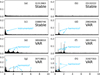 |
Fig. 1 Examples of frequency spectra of stable stars and stars marked as VAR with unclear classification. The horizontal axis shows frequency in c/d, while the vertical axis shows brightness in mmag. The numbers given in the labels are the TIC numbers. |
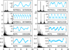 |
Fig. 2 Examples of rotationally variable stars. The horizontal axis shows frequency in c/d, while the vertical axis shows brightness in mmag. The insets show the data in 5 days (four upper panels) and 10 days, respectively. The numbers given in the labels are the TIC numbers. |
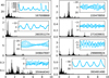 |
Fig. 3 Examples of GDOR stars. The horizontal axis shows frequency in c/d, while the vertical axis shows brightness in mmag. The insets show the data in 10 days. The numbers given in the labels are the TIC numbers. |
3.2 Pulsating stars
Assigning a star with GDOR (gravity-mode, g-mode pulsators), DSCT (pressure-mode, p-mode pulsators), GDOR+DSCT, and DSCT+GDOR (hybrid pulsators) classes can also be challenging task. The first difficulty arises with the definition of the GDOR class, specifically concerning the frequency content and pattern in the frequency spectra. The gravity-mode pulsations of GDOR stars are excited by the convective flux blocking mechanism (Guzik et al. 2000; Dupret et al. 2005). This type of pulsation does not produce equally spaced structures in the frequency domain (harmonics are possible). The GDOR frequencies are usually between 0.3 and 3 c/d (Kaye et al. 1999; Henry et al. 2011), with the most likely position being approximately 1.2-1.3 c/d (see Fig. 1 in Tkachenko et al. 2013). However, when shifted by the rotation, the frequencies can reach up to five cycles per day or even more (Grigahcène et al. 2010). The usually accepted limit to distinguish between g-mode and p-mode pulsators is 5 c/d (Uytterhoeven et al. 2011), but other limits, such as 4 c/d (Antoci et al. 2019), are also being utilised.
The frequency pattern that is characteristic for the GDOR stars is a comb of close, sometimes unresolved, peaks (for example, Balona et al. 2011; Uytterhoeven et al. 2011; Tkachenko et al. 2013, our Fig. 3) that can also be found around harmonics (see Fig. 3 in Saio et al. 2018, and our Fig. 3). This can cause confusion with spotted solar-type stars, which is best apparent in TIC 393491490 in the bottom right panel of Fig. 3. On the other hand, the peaks can also be randomly distributed (e.g., Uytterhoeven et al. 2011; Balona et al. 2011, and TIC 350444342 in the bottom left panel of Fig. 3). We classified stars as GDOR when several peaks were present in the range of approximately 0.3–5 c/d. At the same time, the frequency pattern did not comply with the requirements for rotationally variable stars (see Sect. 3.1). In addition, the amplitude of the frequency peaks has to be larger than 0.1 mmag.
It is important to note that we do not differentiate between slowly pulsating B stars (SPB stars Waelkens et al. 1998; De Cat & Aerts 2002) and GDOR stars as SPB stars are hotter and may contaminate our sample at high temperatures. Additionally, we do not distinguish between low- and high-amplitude GDOR stars (HAGDOR, Paunzen et al. 2020) because the boundary between the two is not well defined, and amplitudes in TESS data may not be reliable due to contamination and data processing. TIC 167008868 is an excellent candidate for HAGDOR (top left panel of Fig. 3) with one of the largest peak-to-peak amplitudes ever observed in HAGDOR (about 0.4 mag in TESS pass band, SPOC routine).
The second important class of pulsating stars among A-F spectral type stars are DSCT pulsators. The pulsations in these low-radial-order p-mode pulsators are excited by the κ mechanism operating in the HeII ionisation zone and by turbulent pressure (Breger 2000; Antoci et al. 2014). As was already mentioned, five cycles per day are usually taken as the border between GDOR and DSCT pulsations (Uytterhoeven et al. 2011). However, some authors use 4 c/d (Antoci et al. 2019). The upper limit is also not firmly defined. Balona (2022) state that there is no sharp transition between roAp (Kurtz 1982) and DSCT stars and that the roAp class should be dropped. In fact, DSCT and roAp stars are different objects and such a comparison concerns only the frequency content (Holdsworth et al. 2024). Nevertheless, we mark a star as a DSCT pulsator if it shows at least one strong peak above 5 c/d. Due to the faster cadence in cycle 3, the Nyquist reflections are not a significant problem, since the Nyquist frequency is 72 c/d, which is well above the dominant frequency for most of the DSCT stars.
The variety of DSCT frequency spectra has been shown many times (e.g. Grigahcène et al. 2010; Uytterhoeven et al. 2011). Examples of frequency spectra of DSCT stars in our sample are in Fig. 4. We can see stars with a single dominant pulsation mode (e.g. TIC 350522254) and stars with a comb of peaks (e.g. TIC 149991210), but also stars with peaks across the whole frequency range (e.g. TIC 299802315).
Ultra-precise space observations revealed that basically all DSCT and GDOR stars show peaks in both regimes (Grigahcène et al. 2010; Uytterhoeven et al. 2011; Balona 2014). Balona (2014) also showed that most of the low frequencies observed in DSCT stars cannot be explained by the non-linear combination of the DSCT modes and by rotation. Thus, the vast majority of stars showing peaks in both DSCT and GDOR regimes are likely hybrids.
The only situation in which it is difficult to identify hybrid pulsators is in stars in which the amplitudes of the frequency peaks are different or the frequency content is poor and the frequency peaks cannot be properly interpreted. There is no commonly accepted amplitude threshold specifying that a particular star is a pure GDOR or DSCT pulsator or a hybrid. The ratio of the amplitudes in both regimes used by Uytterhoeven et al. (2011) and Bradley et al. (2015) are only empirical thresholds (a factor of 5–7 in the amplitude ratio) not saying anything about the hybrid nature. In addition, each author uses a different amplitude limit to consider the frequencies for the classification. All of the mentioned problems add ambiguity to the classification.
As each dataset is unique, we did not adopt any amplitude threshold because even peaks in the sub-mmag regime can be significant. We cannot avoid mixing hybrids with pure DSCT or GDOR stars showing combination peaks without detailed frequency analysis, which is out of the scope of this paper. However, this will be the case in only a minority of stars. For instance, TIC 177035603 (top right-hand panel of Fig. 4) can be classified as a hybrid pulsator with a similar probability as pure DSCT. Similarly, TIC 350444342 in the bottom left panel of Fig. 3 can be also considered as a hybrid pulsator, not a pure GDOR star. Examples of frequency spectra of hybrid pulsators are shown in Fig. 5. The least reliable classification among the shown stars is in TIC 41590715 because the peaks are grouped around 5 c/d and the classification can be all of pure GDOR, pure DSCT, or hybrid pulsator. We give ‘DSCT+LF’ classification to more than 60% of the DSCT stars showing low-amplitude peaks below 5 c/d meaning DSCT stars with low-frequency (LF) peaks with unclear interpretation. Some of these stars can be hybrid stars, but some can also be rotationally variable.
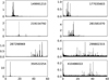 |
Fig. 4 Examples of frequency spectra of DSCT stars. The horizontal axis shows frequency in c/d, while the vertical axis shows brightness in mmag. The numbers given in the labels are the TIC numbers. |
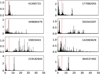 |
Fig. 5 Examples of frequency spectra of hybrid GDOR+DSCT stars. Frequency on the horizontal axis is in c/d, while brightness on the vertical axis is in mmag. The numbers given in the labels are the TIC numbers. The upper four panels show GDOR-dominating hybrids, while the bottom four panels show DSCT-dominating hybrids. The vertical dash-dotted red lines indicate 5 c/d. |
3.3 Contamination and identification issues
The southern TESS CVZ includes the Large Magellanic Cloud (LMC), where many stars are strongly affected by contamination. This is especially problematic due to the low angular resolution of TESS, which is 21″ px−1 (Ricker et al. 2015). Contamination can cause several issues such as distortion of the light curve, mixing of variability, and a decrease in the brightness amplitude. The new data releases of Gaia catalogues (Gaia Collaboration 2018, 2023) led to the identification of redundant entries in the TICv8.0 catalogue (Stassun et al. 2019). In TICv8.2, Paegert et al. (2021) identified ‘phantom’ stars, which arise from diffraction spikes around bright stars, mismatches between different catalogues, and from a combination of two or more fainter stars mimicking one target.
We have found 13 such duplicate entries in our sample by comparing TIC8.0 and TIC8.2 catalogs. The numbers of the duplicates are followed with a ‘p21’ suffix in the ‘Type’ column of Table 4. We also adopted the contamination ratio from Paegert et al. (2021) in column CR, which gives the ratio of contaminating flux and flux of the target star. Furthermore, we have cross-matched the positions from TIC8.0 with the Gaia DR3 catalogue (Gaia Collaboration 2023) within a distance of 105″ (5px). The number of blending stars with a magnitude difference less than 5 mag from the target star is given in the ‘Blend’ column of Table 4. This information can at least help to identify problematic targets. The most contaminated target is TIC 372913472, which has 13 contaminants. Automatic procedures for identifying the true source of the variation signal (e.g., Higgins & Bell 2023) are not effective in our case, as they do not work well with a single frequency. Therefore, each target would require a detailed investigation of the frequency spectrum to get reliable and unambiguous results, which is beyond the scope of this paper.
We also compared the strongest identified frequencies of categorised stars and visually examined the frequency content to identify any obvious contaminants. We considered a star with a larger amplitude peak as the real variable, while the other star with the same frequency but lower amplitude was deemed a duplicate contaminated by the variable star. In Table 4, we provide the TIC number of the real variable (the contaminant) in the ‘Type’ column. There are 20 such cases.
It is important to note that there may be nearby large-amplitude variables, such as eclipsing binaries or Cepheids, located just a few pixels away from the target star. Even when the brightness difference is quite large (more than 5 mag), these variables can contaminate the light of the target and cause false identification of variability. Two examples of this are TIC 358460464 and TIC 277293156, as is shown in Fig. 6. The contaminants are approximately 3 and 2 pixels away from TIC 358460464 and TIC 277293156, respectively. Additionally, the contaminants are 6.2 and 7.3 mag fainter than their respective target stars.
The contaminant of TIC 358460464 is an EW ASAS-SNJ075559.67-644238.3, which is a 15.2-mag star. Only the second and third harmonics of the orbital frequency are apparent in the frequency spectrum of TIC 358460464; thus, we classified it as DSCT (top panel of Fig. 6). On the other hand, three harmonics of the pulsation frequency of ASAS-SNJ053737.66-702553.4 (DCEP star, 15.62 mag) are apparent in the frequency spectrum of TIC 277293156 (bottom panel of Fig. 6), which makes it belong to the ROT category.
In both cases, the classification is wrong, although the contamination ratio is as low as 0.34% in TIC 358460464 (in TIC 277293156 it is 10%). Such wrongly identified stars add noise to the statistics when investigating common characteristics of the stars in particular variability classes. After this finding, we cross-matched our sample with the Gaia DR3 variable star catalogue (Rimoldini et al. 2023) and ASAS-SN variable star catalogue (Jayasinghe et al. 2018) within a 100 arcsecond (5 px) radius and compared the frequencies (and their harmonics) from the catalogues with frequencies identified by us. This helped us to identify 12 contaminants (Table 5), which are typically eclipsing binaries and pulsating stars. We have therefore classified our contaminated stars mostly as eclipsing binaries, DSCT and VAR. Such stars are marked with an additional ‘-C’ in the column type in Table 4.
This exercise underscores the risks of misidentifying and misclassifying variable stars, which is far more common than we previously realised. In the Gaia DR3 variable star catalogue, only 20% of stars in the vicinity of our target stars have had their frequencies determined. Identifying the true variable star is further complicated by the fact that there may be multiple stars within 100 arcseconds of the target (we only considered the brightest one). Additionally, bright stars can contaminate the light from even larger distances than 5 pixels. As a result, we can expect the number of contaminants to be much larger than the 12 cases we list in Table 5.
Finally, there is high probability that many of the sample stars are bound in physical binary or multiple systems. In such cases, the observed variability is a combination of variability of system components. This can also lead to misclassification of the variability type.
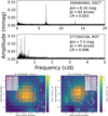 |
Fig. 6 Two identified variable stars that are actually not variable, the light of which is contaminated by nearby stars. The numbers show the TIC identification, variability type, magnitude difference (Δm) between the contaminant and target star, distance of the target from the contaminant (Δr), and the contamination ratio (CR). In the charts generated with TPFPLOTTER (Aller et al. 2020) in the bottom part of the figure, the contaminating stars are numbers 4 and 6 in the left- and right-hand panels, respectively. |
Identification of the contaminating stars.
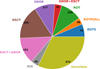 |
Fig. 7 Types of stars identified in our sample. |
4 Results and discussion
We have found that 50.9% of the 1171 stars in our sample (excluding 33 duplicates) show clear variability. This is in agreement with the percentage of variable stars in the northern TESS CVZ (51%, S22). We were able to determine the type of variability in 67.2% of the stars, which is a better performance than in S22, in which only 60% of stars were unambiguously classified. Remaining 372 variable stars were unclassified1. The higher number of data points, longer time span, and increase in the number of sectors observed may have contributed to our better performance in classifying the stars.
The numbers of the classified variable stars are shown in Fig. 7. We have identified a total of 503 pulsating stars, which includes DSCT, GDOR, and their hybrids plus one RRAB star (43% of the variable stars). This count is about 22% less than that of the northern TESS CVZ (S22). We can only speculate about the reasons for the discrepancy.
The diagram in Fig. 8 shows that DSCT and hybrid stars are evenly distributed throughout the empirical IS from Murphy et al. (2019). Pure GDOR stars, on the other hand, are clustered within the theoretical GDOR IS from Dupret et al. (2005), although they can also be found across the entire temperature range. At the hotter end of the scale, GDOR and DSCT stars are likely to mix with SPB and β Cep stars.
As was expected, the ROTS stars are found at the lowest temperatures between 6000–7000 K, while ROTMIELL stars are spread out across the entire temperature range. This indicates that the population of ROTMIELL is a mix of ELL and ROTM stars. The ROT stars tend to prefer temperatures around the cooler GDOR edge but can also be found spread out up to 10 000 K, similar to the distribution found in S22.
We cross-matched our sample with other catalogues within a distance of 21″ (1 px) from our targets to compare the classifications. We used TOPCAT (Taylor 2005) and CDS X-Match service (Boch et al. 2012; Pineau et al. 2020) to cross-match the catalogues. We can use two parameters describing the agreement of the two catalogues. The first parameter is the classification agreement percentage (CAP), which gives the percentage of stars with the same classification in both catalogues. The second parameter is the detection agreement percentage (DAP), which gives the fraction of stars identified and classified as VAR and other variability types in our sample while being assigned with the same variability type or as VAR in the other catalogue.
For instance, if we classify a star as DSCT and the catalogue identifies it as VAR (and vice versa), it will count towards DAP. However, if we classify a star as DSCT and the catalogue identifies it as EW, it will not count. Similarly, if the catalogue gives a variability type, and we do not detect any variability, it will not count. The DAP is useful in reflecting the uncertainty in the classification, as it gives the chance of the classification being correct in at least one of the compared catalogues.
There are 97 sample stars present in the VSX catalogue (Watson et al. 2006). This catalogue is a compilation of variable stars identified in various sky surveys and projects but also by individual observers (for example, NSVS Woźniak et al. 2004, ZTF Chen et al. 2020, and the CzeV catalogue Skarka et al. 2017). However, only 85 of these 97 stars have been categorised. In 15 of the VSX-declared variables, we did not notice any variation. Of the remaining 82 stars that have been classified in the VSX catalogue, we agree with the classification of only 26 stars (32%). The CAP for our classification and VSX is, therefore, 26 out of 97 (27%).
We show examples of where our classification differs from that of the VSX catalogue in Fig. 9. Specifically, we have classified TIC 31925242 (CR Hyi) as a GDOR variable, whereas it is classified as ELL in the VSX catalogue (see the top panel of Fig. 9). Similarly, TIC 350522254 (XY Pic) is classified as DSCT by us2, while it is classified as EW in the VSX catalogue. The data of TIC 350522254 show a beating caused by the presence of two close frequencies at about 6.7 c/d (Fig. 9). For the VSX catalogue, the DAP is 77%.
Of the 84 stars in our sample, 80 are classified as VAR in the ASAS-SN catalogue (Jayasinghe et al. 2018, 2019), while only four are categorised. Among the four categorised stars, one star is classified as GCAS (our ROTM|ELL, TIC 348898673, see Fig. 9), and another star is listed as ROT (our EA, TIC 349480507). However, we did not detect any variation in the remaining two stars that should be classified as GCAS according to Jayasinghe et al. (2018, 2019). Furthermore, we did not detect variation in nine of the declared variable stars. It is worth noting that there is no agreement between our classification and the ASAS-SN catalogue (CAP = 0%). The DAP for our classification and the ASAS-SN catalogue is 85%, but this is only because most of the stars are labelled as VAR in the ASAS-SN catalogue.
We crossmatched our sample of stars also with the Gaia DR3 variables (Rimoldini et al. 2023) within a 21″ radius, and found 219 entries for our stars3. The CAP parameter is 48%, while the DAP is 57%. The high value of CAP is because most stars in our sample have a broad variability type classification in Rimoldini et al. (2023). For example, Gaia DR3 classification ACV|CP|MCP|ROAM|ROAP|SXARI complies with our ROT, ROTS, ROTM|ELL stars, SOLAR LIKE complies with our ROTS, ROT and ROTM|ELL classes, DSCT|GDOR|SXPHE complies with our GDOR, DSCT and their hybrid classes. We found no variability in 35 stars declared as variables in Rimoldini et al. (2023).
In their study, Fetherolf et al. (2023) created a comprehensive list of variable stars from the TESS prime mission by searching for periodicity and variability using the Lomb-Scargle periodogram (Lomb 1976; Scargle 1982). Since we used the same data and analysis method, we expected to obtain similar results. Our sample overlapped with 1141 stars from Fetherolf et al. (2023) catalogue, including 16 duplicates and nine false positives (stars that were blends with faint large-amplitude variables). Unfortunately, Fetherolf et al. (2023) did not provide a classification of the variable stars, so we could only calculate the DAP, which was only 63%. Most of the stars that we disagreed on did not exhibit apparent variability and displayed low-frequency peaks similar to those shown in panel c of Fig. 1. The frequencies of variable stars found by Fetherolf et al. (2023) perfectly matched with frequencies found by us (including our VAR stars). However, in stars that we marked as stable, the frequencies identified by (Fetherolf et al. 2023) differed from the frequencies identified by us. This is an additional argument against assigning these stars as variable.
Forty-four stars from our sample are listed in the binary-star catalogue by Prša et al. (2022). However, we classified three of them not as eclipsing binaries but as ROTM|ELL (TIC 382512330, 306578324, and 141127435) and TIC 142148228 and 150187916 as VAR stars. The CAP and DAP with Prša et al. (2022) are both 89%. This result is no surprise, since variations of eclipsing binaries are characteristic and usually have large amplitudes.
Regarding rotational variable stars, 29 stars from our sample appear in Sikora et al. (2019a). The variations are connected with rotation or orbital motion in only 16 of them. The rotational nature of the other 13 stars is ambiguous. The CAP and DAP are both 55%.
Twelve of our sample stars are listed in Antoci et al. (2019), which deals with DSCT stars. Nine of them were also identified as DSCT (or hybrids) by us, and one of the stars was found to be constant in agreement with Antoci et al. (2019). In TIC 260416268, which was identified as a rot/binary Am star by Antoci et al. (2019), we detected no variability. The same applies to the roAp candidate TIC 238185398. The CAP and DAP are both 83%.
The discrepancies between our results and results from literature arise from the superior characteristics of the TESS data compared to other catalogues meaning better precision, cadence, and often also time span. The agreement in classification with previous studies and catalogues is summarised in Table 6.
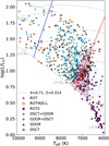 |
Fig. 8 Hertzsprung-Russell diagram showing our categorised stars. The dashed line shows the zero-age main sequence, while the evolutionary tracks are shown with the dash-dotted lines. The empirical boundaries of the DSCT IS are shown with continuous blue and red lines. The ZAMS, evolutionary tracks, and IS boundaries are taken from Murphy et al. (2019). The GDOR instability region (Dupret et al. 2005) is shown with the shaded area limited by the dotted lines. All the stars in our sample including non-variable stars are shown with grey dots. |
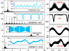 |
Fig. 9 Stars with incorrect classification in the catalogues. The left panels show the frequency spectra with the part of the time series (the catalogue classification is given together with the TIC number), while the right-hand panels show the data phase-folded with the dominant frequency together with the correct variability type. |
Agreement (1st column) in per cent of our classification with the large catalogues and dedicated studies.
5 Conclusions
We carefully classified variable stars using data from TESS from cycles 1 and 3. This data is useful for detecting fast variations, such as DSCT pulsations, as well as variations that occur over several days. We discussed the limitations of our classifications, including the general shortcomings in variable stars classification. Furthermore, we compared our results with existing databases and variable star catalogues.
We confirm the previous issues with the classification of rotationally variable stars and hours- to days-long pulsations of GDOR type. It is also often difficult to distinguish between ellipsoidal and/or contact binary variables and spotted stars without additional information. Additionally, the classification can be influenced by nearby stars, and the level of contamination depends on the distance of the contaminating star, the amplitude of variations, and the difference in brightness. This mainly affects the classification of rotationally variable stars and stars that show a combination of different types of variation.
We found intriguing discrepancies in the classification in variable stars catalogues that can be up to 100%. To address this issue, we have introduced two parameters – CAP and DAP. The CAP reflects the classification, while the DAP concerns the detection of variability without a specific variability type. Our results show that we have a relatively good agreement with the Gaia catalogue (CAP = 48%, Rimoldini et al. 2023). The best agreement is with the studies dedicated to particular variability types. For instance, the agreement of our classification is almost 90% with the database of eclipsing binaries (Prša et al. 2022) and 83% in the case of DSCT variables (Antoci et al. 2019). Surprisingly, the agreement of our results with a study by Fetherolf et al. (2023), which is also based on the TESS data, is only 63%. We have also demonstrated that large-amplitude variables can contaminate the light of the target stars up to 100 arcseconds from the star, which can lead to incorrect identification and classification.
It has been shown that classifying variable stars is a complex task and may produce ambiguous or incorrect results. It is not advisable to blindly use samples of variable stars without individually checking each star. This is especially important in the usage of samples based on automatic classifiers. To create reliable catalogues of variable stars, it is necessary to analyze not only single-channel photometric observations but also multicolour and spectroscopic observations, and to estimate reddening and distance. Additionally, one must be very careful in handling contamination. Only then can we be confident that the variations of specific objects are caused by the proposed effect(s).
The first PLATO mission field (LOPS2, Nascimbeni et al. 2022) will include the southern TESS CVZ. Our classification represents a good starting point for studies of stellar variability in the PLATO field.
Acknowledgements
M.S. acknowledges the support by Inter-transfer grant no LTT-20015. This paper includes data collected with the TESS mission. Funding for the TESS mission is provided by the NASA Explorer Program. Funding for the TESS Asteroseismic Science Operations Centre is provided by the Danish National Research Foundation (Grant agreement no.: DNRF106), ESA PRODEX (PEA 4000119301) and Stellar Astrophysics Centre (SAC) at Aarhus University. We thank the TESS team and staff and TASC/TASOC for their support of the present work. We also thank the TASC WG4 team for their contribution to the selection of targets for 2-min observations. The TESS data were obtained from the MAST data archive at the Space Telescope Science Institute (STScI).
References
- Aller, A., Lillo-Box, J., Jones, D., Miranda, L. F., & Barcelo Forteza, S. 2020, A&A, 635, A128 [NASA ADS] [CrossRef] [EDP Sciences] [Google Scholar]
- Antoci, V., Cunha, M., Houdek, G., et al. 2014, ApJ, 796, 118 [Google Scholar]
- Antoci, V., Cunha, M. S., Bowman, D. M., et al. 2019, MNRAS, 490, 4040 [Google Scholar]
- Audenaert, J., Kuszlewicz, J. S., Handberg, R., et al. 2021, AJ, 162, 209 [NASA ADS] [CrossRef] [Google Scholar]
- Audenaert, J., & Tkachenko, A. 2022, A&A, 666, A76 [NASA ADS] [CrossRef] [EDP Sciences] [Google Scholar]
- Balona, L. A. 2014, MNRAS, 437, 1476 [NASA ADS] [CrossRef] [Google Scholar]
- Balona, L. A. 2022, MNRAS, 510, 5743 [NASA ADS] [CrossRef] [Google Scholar]
- Balona, L. A., Guzik, J. A., Uytterhoeven, K., et al. 2011, MNRAS, 415, 3531 [Google Scholar]
- Barentsen, G., & Lightkurve Collaboration. 2020, AAS Meeting Abstracts, 235, 409.04 [NASA ADS] [Google Scholar]
- Boch, T., Pineau, F., & Derriere, S. 2012, ASP Conf. Ser., 461, 291 [NASA ADS] [Google Scholar]
- Borucki, W. J., Koch, D., Basri, G., et al. 2010, Science, 327, 977 [Google Scholar]
- Bradley, P. A., Guzik, J. A., Miles, L. F., et al. 2015, AJ, 149, 68 [CrossRef] [Google Scholar]
- Breger, M. 2000, ASP Conf. Ser., 210, 3 [NASA ADS] [Google Scholar]
- Chen, X., Wang, S., Deng, L., et al. 2020, ApJS, 249, 18 [NASA ADS] [CrossRef] [Google Scholar]
- Dall, T. H. 2005, Information Bull. Variable Stars, 5617, 1 [NASA ADS] [Google Scholar]
- De Cat, P., & Aerts, C. 2002, A&A, 393, 965 [NASA ADS] [CrossRef] [EDP Sciences] [Google Scholar]
- Dupret, M. A., Grigahcène, A., Garrido, R., Gabriel, M., & Scuflaire, R. 2005, A&A, 435, 927 [NASA ADS] [CrossRef] [EDP Sciences] [Google Scholar]
- Faigler, S., & Mazeh, T. 2011, MNRAS, 415, 3921 [Google Scholar]
- Fetherolf, T., Pepper, J., Simpson, E., et al. 2023, ApJS, 268, 4 [NASA ADS] [CrossRef] [Google Scholar]
- Gaia Collaboration (Brown, A. G. A., et al.) 2018, A&A, 616, A1 [NASA ADS] [CrossRef] [EDP Sciences] [Google Scholar]
- Gaia Collaboration (Vallenari, A., et al.) 2023, A&A, 674, A1 [NASA ADS] [CrossRef] [EDP Sciences] [Google Scholar]
- Green, M. J., Maoz, D., Mazeh, T., et al. 2023, MNRAS, 522, 29 [CrossRef] [Google Scholar]
- Grigahcène, A., Antoci, V., Balona, L., et al. 2010, ApJ, 713, L192 [Google Scholar]
- Guzik, J. A., Kaye, A. B., Bradley, P. A., Cox, A. N., & Neuforge, C. 2000, ApJ, 542, L57 [Google Scholar]
- Henry, G. W., Fekel, F. C., & Henry, S. M. 2011, AJ, 142, 39 [NASA ADS] [CrossRef] [Google Scholar]
- Higgins, M. E., & Bell, K. J. 2023, AJ, 165, 141 [NASA ADS] [CrossRef] [Google Scholar]
- Holdsworth, D. L., Cunha, M. S., Lares-Martiz, M., et al. 2024, MNRAS, 527, 9548 [Google Scholar]
- Huang, C. X., Vanderburg, A., Pál, A., et al. 2020a, Res. Notes Am. Astron. Soc., 4, 204 [Google Scholar]
- Huang, C. X., Vanderburg, A., Pál, A., et al. 2020b, Res. Notes Am. Astron. Soc., 4, 206 [Google Scholar]
- Iwanek, P., Soszynski, I., Kozlowski, S., et al. 2022, ApJS, 260, 46 [NASA ADS] [CrossRef] [Google Scholar]
- Jayasinghe, T., Kochanek, C. S., Stanek, K. Z., et al. 2018, MNRAS, 477, 3145 [Google Scholar]
- Jayasinghe, T., Stanek, K. Z., Kochanek, C. S., et al. 2019, MNRAS, 485, 961 [Google Scholar]
- Jenkins, J. M., Twicken, J. D., McCauliff, S., et al. 2016, SPIE Conf. Ser., 9913, 99133E [Google Scholar]
- Kaye, A. B., Handler, G., Krisciunas, K., Poretti, E., & Zerbi, F. M. 1999, PASP, 111, 840 [Google Scholar]
- Kurtz, D. W. 1982, MNRAS, 200, 807 [NASA ADS] [CrossRef] [Google Scholar]
- Lightkurve Collaboration (Cardoso, J. V. d. M., et al.) 2018, Astrophysics Source Code Library [record ascl:1812.013] [Google Scholar]
- Lomb, N. R. 1976, Ap&SS, 39, 447 [Google Scholar]
- Murphy, S. J., Hey, D., Van Reeth, T., & Bedding, T. R. 2019, MNRAS, 485, 2380 [NASA ADS] [CrossRef] [Google Scholar]
- Nascimbeni, V., Piotto, G., Börner, A., et al. 2022, A&A, 658, A31 [NASA ADS] [CrossRef] [EDP Sciences] [Google Scholar]
- Paegert, M., Stassun, K. G., Collins, K. A., et al. 2021, arXiv e-prints [arXiv:2108.04778] [Google Scholar]
- Paunzen, E., Bernhard, K., Hümmerich, S., et al. 2020, MNRAS, 499, 3976 [NASA ADS] [CrossRef] [Google Scholar]
- Pineau, F.-X., Boch, T., Derrière, S., & Schaaff, A. 2020, ASP Conf. Ser., 522, 125 [NASA ADS] [Google Scholar]
- Prša, A., Kochoska, A., Conroy, K. E., et al. 2022, ApJS, 258, 16 [CrossRef] [Google Scholar]
- Ricker, G. R., Winn, J. N., Vanderspek, R., et al. 2015, J. Astron. Telesc. Instrum. Syst., 1, 014003 [Google Scholar]
- Rimoldini, L., Holl, B., Gavras, P., et al. 2023, A&A, 674, A14 [NASA ADS] [CrossRef] [EDP Sciences] [Google Scholar]
- Saio, H., Bedding, T. R., Kurtz, D. W., et al. 2018, MNRAS, 477, 2183 [Google Scholar]
- Samus, N. N., Kazarovets, E. V., Durlevich, O. V., Kireeva, N. N., & Pastukhova, E. N. 2009, VizieR Online Data Catalog: B/gcvs [Google Scholar]
- Scargle, J. D. 1982, ApJ, 263, 835 [Google Scholar]
- Sikora, J., David-Uraz, A., Chowdhury, S., et al. 2019a, MNRAS, 487, 4695 [Google Scholar]
- Sikora, J., Wade, G. A., Power, J., & Neiner, C. 2019b, MNRAS, 483, 3127 [NASA ADS] [CrossRef] [Google Scholar]
- Skarka, M., Mašek, M., Brát, L., et al. 2017, Open European J. Variab. Stars, 185, 1 [NASA ADS] [Google Scholar]
- Skarka, M., Žák, J., Fedurco, M., et al. 2022, A&A, 666, A142 [NASA ADS] [CrossRef] [EDP Sciences] [Google Scholar]
- Soszynski, I., Pawlak, M., Pietrukowicz, P., et al. 2016, Acta Astron., 66, 405 [NASA ADS] [Google Scholar]
- Soszynski, I., Udalski, A., Wrona, M., et al. 2019, Acta Astron., 69, 321 [NASA ADS] [Google Scholar]
- Stassun, K. G., Oelkers, R. J., Paegert, M., et al. 2019, AJ, 158, 138 [Google Scholar]
- Taylor, M. B. 2005, ASP Conf. Ser., 347, 29 [Google Scholar]
- Tkachenko, A., Aerts, C., Yakushechkin, A., et al. 2013, A&A, 556, A52 [NASA ADS] [CrossRef] [EDP Sciences] [Google Scholar]
- Twicken, J. D., Chandrasekaran, H., Jenkins, J. M., et al. 2010, SPIE Conf. Ser., 7740, 77401U [Google Scholar]
- Uytterhoeven, K., Moya, A., Grigahcène, A., et al. 2011, A&A, 534, A125 [CrossRef] [EDP Sciences] [Google Scholar]
- Waelkens, C., Aerts, C., Kestens, E., Grenon, M., & Eyer, L. 1998, A&A, 330, 215 [NASA ADS] [Google Scholar]
- Watson, C. L., Henden, A. A., & Price, A. 2006, Soc. Astron. Sci., 25, 47 [Google Scholar]
- Wenger, M., Ochsenbein, F., Egret, D., et al. 2000, A&AS, 143, 9 [NASA ADS] [CrossRef] [EDP Sciences] [Google Scholar]
- Wozniak, P. R., Vestrand, W. T., Akerlof, C. W., et al. 2004, AJ, 127, 2436 [NASA ADS] [CrossRef] [Google Scholar]
Considering ROTMIELL stars as categorised stars.
The variability type DSCT of XY Pic was already discussed by Dall (2005).
By omitting three stars that are apparent blends with other stars in our sample.
All Tables
Number of stars in particular temperature ranges (based on temperatures from TIC, Stassun et al. 2019).
Description of variability types used in this work together with the basic light-curve and frequency spectra characteristics.
Agreement (1st column) in per cent of our classification with the large catalogues and dedicated studies.
All Figures
|
Fig. 1 Examples of frequency spectra of stable stars and stars marked as VAR with unclear classification. The horizontal axis shows frequency in c/d, while the vertical axis shows brightness in mmag. The numbers given in the labels are the TIC numbers. |
| In the text | |
|
Fig. 2 Examples of rotationally variable stars. The horizontal axis shows frequency in c/d, while the vertical axis shows brightness in mmag. The insets show the data in 5 days (four upper panels) and 10 days, respectively. The numbers given in the labels are the TIC numbers. |
| In the text | |
|
Fig. 3 Examples of GDOR stars. The horizontal axis shows frequency in c/d, while the vertical axis shows brightness in mmag. The insets show the data in 10 days. The numbers given in the labels are the TIC numbers. |
| In the text | |
|
Fig. 4 Examples of frequency spectra of DSCT stars. The horizontal axis shows frequency in c/d, while the vertical axis shows brightness in mmag. The numbers given in the labels are the TIC numbers. |
| In the text | |
|
Fig. 5 Examples of frequency spectra of hybrid GDOR+DSCT stars. Frequency on the horizontal axis is in c/d, while brightness on the vertical axis is in mmag. The numbers given in the labels are the TIC numbers. The upper four panels show GDOR-dominating hybrids, while the bottom four panels show DSCT-dominating hybrids. The vertical dash-dotted red lines indicate 5 c/d. |
| In the text | |
|
Fig. 6 Two identified variable stars that are actually not variable, the light of which is contaminated by nearby stars. The numbers show the TIC identification, variability type, magnitude difference (Δm) between the contaminant and target star, distance of the target from the contaminant (Δr), and the contamination ratio (CR). In the charts generated with TPFPLOTTER (Aller et al. 2020) in the bottom part of the figure, the contaminating stars are numbers 4 and 6 in the left- and right-hand panels, respectively. |
| In the text | |
|
Fig. 7 Types of stars identified in our sample. |
| In the text | |
|
Fig. 8 Hertzsprung-Russell diagram showing our categorised stars. The dashed line shows the zero-age main sequence, while the evolutionary tracks are shown with the dash-dotted lines. The empirical boundaries of the DSCT IS are shown with continuous blue and red lines. The ZAMS, evolutionary tracks, and IS boundaries are taken from Murphy et al. (2019). The GDOR instability region (Dupret et al. 2005) is shown with the shaded area limited by the dotted lines. All the stars in our sample including non-variable stars are shown with grey dots. |
| In the text | |
|
Fig. 9 Stars with incorrect classification in the catalogues. The left panels show the frequency spectra with the part of the time series (the catalogue classification is given together with the TIC number), while the right-hand panels show the data phase-folded with the dominant frequency together with the correct variability type. |
| In the text | |
Current usage metrics show cumulative count of Article Views (full-text article views including HTML views, PDF and ePub downloads, according to the available data) and Abstracts Views on Vision4Press platform.
Data correspond to usage on the plateform after 2015. The current usage metrics is available 48-96 hours after online publication and is updated daily on week days.
Initial download of the metrics may take a while.