| Issue |
A&A
Volume 666, October 2022
|
|
|---|---|---|
| Article Number | A141 | |
| Number of page(s) | 20 | |
| Section | Extragalactic astronomy | |
| DOI | https://doi.org/10.1051/0004-6361/202243733 | |
| Published online | 18 October 2022 | |
Revealing impacts of stellar mass and environment on galaxy quenching
1
Astronomical Institute, Graduate School of Science, Tohoku University, 6–3 Aoba, Sendai 980-8578, Japan
e-mail: This email address is being protected from spambots. You need JavaScript enabled to view it.
2
Graduate Program on Physics for the Universe (GP-PU), Tohoku University, 6–3 Aoba, Sendai 980-8578, Japan
3
Kalvi Institute for the Physics and Methematics of the Universe, University of Tokyo, 5-1-5 Kashiwanoha, Kashiwa, Chiba 277-8583, Japan
Received:
8
April
2022
Accepted:
29
July
2022
Abstract
Aims. Galaxy quenching is a critical step in galaxy evolution. In this work, we present a statistical study of galaxy quenching in 17 cluster candidates at 0.5 < z < 1.0 in the COSMOS field.
Methods. We selected cluster members with a wide range of stellar masses and environments to study their mass and environment dependence. Member galaxies are classified into star-forming, quiescent, and recently quenched galaxies (RQGs) using the rest-frame UVJ diagram. We further separated fast- and slow-quenching RQGs by model evolutionary tracks on the UVJ diagram. We defined the quenching efficiency as the ratio of RQGs to star-forming galaxies and the quenching stage as the ratio of RQGs to quiescent galaxies to quantify the quenching processes.
Results. We find that quenching efficiency is enhanced by both higher stellar mass and denser environment. Massive or dense environment galaxies quench earlier. Slow quenching is more dominant for massive galaxies and at lower redshifts, but no clear dependence on the environment is found. Our results suggest that low-mass galaxies in dense environments are likely quenched through a short timescale process such as ram pressure stripping, while massive galaxies in a sparse environment are mostly quenched by a longer timescale process. Using the line strength of Hδ and [OII], we confirmed that our UVJ method to select RQGs agrees with high S/N DEIMOS spectra. However, we caution that the visibility time (duration of a galaxy’s stay in the RQG region on the UVJ diagram) may also depend on mass or environment. The method introduced in this work can be applied to RQG candidates for future statistical RQG spectroscopic surveys. The systematic spectroscopic RQG study will disentangle the degeneracy between visibility time and quenching properties.
Key words: galaxies: evolution / galaxies: clusters: general / galaxies: star formation / galaxies: high-redshift / galaxies: photometry
© Z. Mao et al. 2022
 Open Access article, published by EDP Sciences, under the terms of the Creative Commons Attribution License (https://creativecommons.org/licenses/by/4.0), which permits unrestricted use, distribution, and reproduction in any medium, provided the original work is properly cited.
This article is published in open access under the Subscribe-to-Open model. This email address is being protected from spambots. You need JavaScript enabled to view it. to support open access publication.
1. Introduction
Deep surveys have transformed our view of the distant Universe, allowing us to constrain the process of galaxy formation and evolution over the past 13 billion years of cosmic history. The cosmic star formation rate density comes to a peak at z ∼ 2 − 3, and then it declines as the Universe ages until the present day (Lilly et al. 1996; Karim et al. 2011; Burgarella et al. 2013; Madau & Dickinson 2014; Khostovan et al. 2015). This decline in star formation is called galaxy quenching, an essential step in galaxy evolution. Although there have been many efforts to understand quenching mechanisms, there is still a lack of conclusive results.
Quenching is a process where star-forming galaxies (SFGs) transform into quiescent galaxies (QGs). The transitional population between SFGs and QGs are recently quenched galaxies (RQGs), which are ideal for studying the quenching process (Wu et al. 2020). The RQGs are still in the quenching process or have just finished (Newberry et al. 1990; Wild et al. 2009; French et al. 2018). This nature makes them capable of delivering information about the physical processes during quenching. RQGs have quenched their star formation in the past few ten million years to a few billion years (Couch & Sharples 1987; Poggianti et al. 2009), but they still contain a large fraction of relatively young A-type stars. This particular stellar composition adds strong Balmer absorption lines to the passive galaxy spectrum (Dressler & Gunn 1983; Couch & Sharples 1987; Wild et al. 2009). In previous studies, this population is mostly referred to as post-starburst galaxies (PSBs), which means galaxies that have experienced a starburst episode followed by a fast quenching. However, this starburst phase is not essential for quenching, and the quenching timescale varies for each galaxy (Poggianti et al. 2009). Therefore, we use recently quenched galaxy in this work as a more precise name for this population.
There are two key parameters for describing galaxy quenching, mass and environment, as the red fraction of galaxies is known to correlate strongly with these two parameters (Peng et al. 2010; Sobral et al. 2011; Muzzin et al. 2012; Darvish et al. 2016). The physical mechanisms of quenching are correspondingly categorised into mass-dependent and environment-dependent types.
Among the stellar mass-driven quenching, the most studied mechanism is active galactic nucleus (AGN) feedback (Best et al. 2005; Hopkins et al. 2005; Kaviraj et al. 2007; Diamond-Stanic et al. 2012; Belli et al. 2021), which is also studied in simulations (e.g. Dubois et al. 2013; Beckmann et al. 2017; Weinberger et al. 2017; Piotrowska et al. 2022; Shi et al. 2022; Xu et al. 2022). The quasar host AGNs show evidence of having strong outflows in observation (Dai et al. 2008; Tombesi et al. 2010). AGN outflows cause expulsion of the gas from the gravitational bound of the system, and hence reduce the subsequent star formation activity in their host galaxies (Debuhr et al. 2012; Combes 2017). AGNs can also heat up the cool gas of the interstellar medium, hence preventing the galaxy from forming new stars (Croton et al. 2006; Man & Belli 2018; Zinger et al. 2020). Supernovae feedback is another primary mechanism of mass-dependent quenching that mainly acts on low-mass galaxies. High-energy ejections and superwinds take away the cold gas, stopping further star formation activity (Dekel & Silk 1986; Dekel & Woo 2003).
On the other hand, quenching mechanisms related to interactions between galaxies and their environment, for example other galaxies, the intracluster medium (ICM), and the intergalactic medium (IGM), are considered environmental quenching. A widely established mechanism of environmental quenching is strangulation, also known as starvation (Larson et al. 1980). The virial shocks from the halo heat up the cool gas, ceasing the galaxies’ gas supply. The star formation will then be quenched due to the lack of fuel (Bekki et al. 2002; Man & Belli 2018). Galaxy mergers can be another mechanism of environmental quenching. In particular, major mergers can trigger starbursts, which are followed by rapid consumption of all remaining cool gas (Mihos & Hernquist 1996; Gabor et al. 2010; Man & Belli 2018). In addition, when galaxies encounter each other at high speed, their potential wells will interact, causing gravitational shocks. Even though the effect of individual encounters may not be large, the repeated process in high-density environments would make a significant impact on galaxies. This process is known as galaxy harassment (Moore et al. 1996, 1998). Galaxy harassment leads to instability of galaxy morphology and change in the distribution of material, driving gas into central regions (Moore et al. 1999; Boselli & Gavazzi 2006). Galaxies will be quenched after a starburst consumes their gas. Ram pressure stripping is also an effective environmental quenching mechanism (Ma et al. 2008; Bekki 2009; Roediger et al. 2014). As galaxies move through the ICM in cluster cores, the wind from the ICM will strip the gas from them (Gunn & Gott 1972; Balogh et al. 2000; Steinhauser et al. 2016).
Many mechanisms that probably lead to quenching have been proposed, and surely we need some parameters to discriminate between these mechanisms. One of such critical parameters we are looking for is the quenching timescale, which varies from one mechanism to another. Most of these timescales are obtained from simulations (Wright et al. 2019; Wetzel et al. 2013; Walters et al. 2022). Among mass-dependent quenching mechanisms, the supernova feedback is a strong physical process that quickly quenches star formation in ∼0.1 Gyr (Ceverino & Klypin 2009). On the other hand, the AGN feedback timescale is still under debate. Quasar mode AGN feedback is a strong process. Quasars’ lifetimes are not long (< 0.1 Gyr, Hopkins et al. 2006), and the gas outflow driven by quasars can quench star formation at million-year-level timescales (Smethurst et al. 2021). On the other hand, the radio mode of AGN feedback is a slow process (Best et al. 2005); it takes up to and beyond 1 Gyr to establish a balance between cooling and heating to reach a low star formation rate phase (Fabian 2012). In Schawinski et al. (2014) the authors maintain that the timescale of AGN feedback leading to a quenching can be related to the host galaxy type. Furthermore, Hirschmann et al. (2017) simulated the star formation history (SFH) of galaxies with AGN and found that the quenching timescale can have a wide range, from a few hundred Myr to a few Gyr. For environmental quenching mechanisms, strangulation is a long-term process that lasts a few billion years (Peng et al. 2015). Merger-driven quenching does not happen directly after galaxy merger events; a median delay time of 1.5 Gyr is expected, and the timescale varies over a wide range (Rodríguez Montero et al. 2019). Ram pressure stripping is a rapid type of quenching, with a timescale of ∼0.2 Gyr (Steinhauser et al. 2016). Thus, we can use the quenching timescale to determine some of the physical mechanisms involved.
To study the quenching process, the main drawback of current RQG works is the lack of observations. Due to their intrinsic short-lived nature, RQGs are rare objects (Tran et al. 2004; Le Borgne et al. 2006; Kaviraj et al. 2007), and we still lack a large spectroscopic sample to carry out systematic studies. Although RQG spectra can provide direct information and strict constraints on their physical properties and SFH, only a limited number of RQG spectra exist at high redshifts (e.g. Pracy et al. 2010; Maltby et al. 2016; D’Eugenio et al. 2020). Increasing the spectroscopic sample is critical, and for this purpose we first need to make a large photometric sample of RQG candidates to feed spectroscopic follow-up observations. Moreover, such a statistical photometrically selected sample of RQG candidates is essential for us to explore the quenching processes prior to spectroscopic studies. As the quenching process is strongly correlated with mass and environment, a systematic study of RQGs must cover a wide range of masses and environments. Therefore, we require a sample of RQGs extending from cluster cores to general fields in order to understand environmental quenching. There are some previous works that study the environment-dependent quenching using the post-starburst galaxy (PSB) population, which belongs to the RQG population (e.g. Socolovsky et al. 2018; Paccagnella et al. 2017, 2019). They study the environment-dependent quenching by estimating the PSB fraction or number in different environments (e.g. cluster, group, or field; distance to cluster centre). These studies prove that the PSBs tend to reside in denser environments. Their results also suggest that there should be various quenching mechanisms in different environments (Paccagnella et al. 2017). In clusters, fast quenching processes, such as ram pressure stripping, are enhanced. In sparse environments, galaxy mergers and interactions produce PSBs (Socolovsky et al. 2018; Paccagnella et al. 2019). There are also works on the mass dependence of galaxy quenching. McNab et al. (2021) studied the mass dependence of quenching for transitional populations (similar to RQGs) using spectroscopic data from the GOGREEN survey (Balogh et al. 2017). Their results support the scenario of pre-processing in the group or proto-cluster environment for massive galaxies and the fast quenching during infall for lower mass galaxies. The GOGREEN survey contains spectra of many cluster galaxies with secure redshift at 0.8 < z < 1.5, which will improve the study of transitional populations in the future.
In this work we present a systematic study of RQGs based on multi-band photometric data in 17 cluster candidates in the COSMOS field at 0.5 < z < 1.0. Our aim is to develop an efficient method of selecting RQGs from photometric surveys (e.g. HSC-SSP, Aihara et al. 2019) to prepare for the coming spectroscopic RQG survey using the Prime Focus Spectrograph (PFS, Tamura et al. 2018) on Subaru. We selected our RQG sample with the rest-frame UVJ colour-colour diagram and confirmed some of the proposed quenching mechanisms using this sample. With the current photometrically selected RQGs, we conducted basic analyses on mass and environment dependence of galaxy quenching and obtained some preliminary results. This paper is structured as follows. In Sect. 2 we present the photometric data we used and the cluster galaxy sample we selected. In Sect. 3 we present the method we use to classify RQGs and correct for possible projection effects. In Sect. 4 we display our results of quenching efficiency, quenching stage, and quenching timescale. In Sect. 5 we discuss the possible contamination and incompleteness of our RQG selection, compare our results with previous works, and then attempt to interpret the results we obtained from the current sample. An H0 = 69.6 km s−1 Mpc, ΩM = 0.286 and ΩΛ = 0.714 cosmology is used. All cosmology calculations are conducted by the cosmology calculator from Wright (2006). All magnitudes presented in this paper are defined in the AB magnitude system.
2. Dataset and sample
In Sect. 2.1 we describe the photometric data we use in this study. In Sect. 2.2 we describe how we selected our sample galaxies to study the quenching processes.
2.1. The COSMOS2015 catalogue
The photometric data that we use in this work is part of the COSMOS2015 catalogue (Laigle et al. 2016). This catalogue mainly combines 26 bands from optical to infrared wavelengths of galaxies in the COSMOS field. It offers deep (mAB ∼ 25 − 26 mag) data covering a relatively large area of 2 deg2. As we require near-infrared (NIR) photometry to estimate the rest-frame J-band magnitude, the data we use is limited to the central ∼1.4 deg2 of the COSMOS field. In this work we use B, V, r, i+, z++ taken with Suprime-Cam/Subaru; Y, J, H, Ks bands taken with VIRCAM/VISTA; and 3.6 μm, 4.5 μm taken with IRAC/Spitzer. Broad-band B, V, r, i+ data are from the previous data release (Capak et al. 2007; Ilbert et al. 2009). Broad z++ band data are taken with new upgraded CCDs. For each optical band, image PSFs are homogenised so that tile-to-tile variations can reach minimisation (Capak et al. 2007). NIR Y, J, H, Ks band data are part of the UltraVISTA survey, and the data combined with the COSMOS2015 catalogue was released in UltraVISTA-DR2, which is much deeper in ultra-deep stripes compared to DR1 (McCracken et al. 2012). The IRAC 3.6 μm, 4.5 μm data are a combination of several programmes observing the COSMOS field using Spitzer (Capak 2016). We corrected for foreground galactic extinction according to the catalogue included reddening value EBV (=E(B − V)) for each object and foreground extinction factor Ff (Allen 1976) according to Laigle et al. (2016):
 (1)
(1)
In this work we use photometric redshift and stellar mass estimation results from Laigle et al. (2016). In that work spectral energy distribution (SED) fitting and photometric redshift estimation are performed with the LEPHARE code (Arnouts et al. 2002; Ilbert et al. 2006). They use a set of 31 templates, including spiral and elliptical galaxies from Polletta et al. (2007) together with 12 templates of young blue SFGs generated by the Bruzual & Charlot (2003) models. Dust attenuation is added as a free parameter; 3″ aperture magnitudes are adopted since they provide slightly better photometric redshift. The code performs χ2 analysis between template predicted and observed fluxes. Stellar masses are then derived by the method of Ilbert et al. (2015), using a spectral library generated by the Bruzual & Charlot (2003) model. The Chabrier (2003) initial mass function is assumed.
A 97% confidence-level spectroscopic redshift sample is obtained from Lilly et al. (2007) to examine the reliability of photometric redshift. The precision of photometric redshift is estimated using normalised median absolute deviation (NMAD, Hoaglin et al. 1983), which is defined as 1.48 × median(|zp − zs|/(1 + zs)), where zp refers to photometric redshift and zs refers to spectroscopic redshift. The dispersion of NMAD of the spectroscopically confirmed sample is σ = 0.021. Since the width of the redshift slices we used in this study is 0.1, this sigma level is precise enough for our further study. This work focuses on the redshift range z ∼ 0.5 − 1.0, where we have more confirmation of photometric redshift and higher mass completeness (see Sect. 2.2). Moreover, in this range, the UVJ selection criteria are not affected by redshift; hence, we can apply the same UVJ selection region for the whole sample (more information in Appendix A).
2.2. Sample selection
In this section we describe how we select galaxy cluster candidates and their member galaxies.
We followed the steps in Laigle et al. (2016) to obtain mass completeness for this sample. For each galaxy the mass required for it to be observed (Mlim) is determined based on Ks magnitude and stellar mass M according to the following equation:
 (2)
(2)
For each galaxy, the 5σ limiting magnitude (Ks, lim) is used to estimate the stellar mass required for the galaxy to be observed (Mlim). Then in each redshift bin the mass completeness is set to the Mlim value that contains 90% of the galaxies. The qualitative conclusions we draw remain unchanged when we apply a slightly higher mass cut, such as 95%. In the overall sample, we remove galaxies without a stellar mass estimation and adopt the most conservative mass limit in the highest redshift bin at Mlim = 109.8 M⊙. All further analyses are carried out for galaxies with stellar masses higher than the mass limit based on the SED fitting.
We then select galaxies with type flag = 0 (galaxy type). Since we use five optical bands from Subaru and four UVista near-infrared bands to calculate rest-frame UVJ colour, we require our target galaxy to cover at least two optical and two NIR bands to ensure the accuracy of rest-frame colour estimation. After these selections, we have 31 983 galaxies. We further select our analysis sample and field sample from these galaxies.
In order to study the environmental dependence of galaxy properties in an unbiased way, we select our sample galaxies from the cluster cores to the outskirts. Thus, our first step is to search for galaxy cluster candidates at 0.5 < z < 1.
2.2.1. Overdensity identification
In this study we select overdensity regions based on the aperture density method, computing the aperture density (i.e. the number density of galaxies in a certain aperture) across our field using 1 Mpc radius apertures. Since there is no complete cluster catalogue at this redshift range, we choose to identify our own cluster candidates to remain consistent throughout this work in the selection and analysis of our cluster and field samples.
We first slice the overall sample into five redshift bins with a width of Δz = 0.1 each. Then we calculate the aperture density distribution for each slice and make the aperture density maps (e.g. Fig. 1) by placing 1 Mpc radius apertures on 1 Mpc × 1 Mpc grids that cover the whole COSMOS field. We adopt this aperture size to capture the overdensity on the cluster scale, since 1 Mpc is similar to the radius of a 1014 M⊙ level cluster (Chiang et al. 2013). Then we define σ as the scatter of densities in all apertures. Regions with > 3σ overdensity (i.e. the density is at least 3σ higher than the average density) are selected as possible cluster candidates. In some cases, the redshift distribution of cluster members is too close to the edge of the redshift slice under scrutiny. Thus, we shift the redshift bin by z ∼ 0.05 to include the majority of the members (see more in Sect. 2.2.3). We selected 37 overdensity regions in all redshift bins, 8 of which are the same overdensity regions at different redshifts. As a result, we found 29 different overdensity regions in 0.5 < z < 1.0.
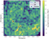 |
Fig. 1. Aperture density map of a redshift slice at z ∼ 0.5 − 0.6. The colours show aperture density in the logarithm scale. The red contours indicate the edge of 3σ peaks, and the blue contours the edge of 1σ regions. The area outside the 1σ contours is identified as field. This kind of density map is plotted for all redshift slices to select cluster candidates and construct the field sample, which is used to make a statistical subtraction of the field average density. Stars indicate the confirmed cluster candidates analysed in this work. |
2.2.2. Member galaxy selection
We adopted 1 Mpc radius apertures to select overdensities, but they cannot trace fine structures and local environments within cluster candidates. Thus, we used the local density, Σ5, to probe the local environment; Σ5 is defined as the average density within a circle centred at a given position with a radius of the distance between the central point and its fifth nearest neighbour. We note that we should not use average Σ5 as the overall field average density due to the uncertainty of photometric redshift. In redshift confirmed overdensities (see Sect. 2.2.3), the nearest neighbours have lower probabilities of being foreground or background galaxies. However, in low-density field areas, the impact of projection effects is strong and cannot be corrected. To determine the centre of the cluster candidates, the Σ5 values are calculated on 0.01 Mpc steps covering the 1 Mpc × 1 Mpc square region centring the peak of aperture density in each cluster candidate. The Σ5 peaks within the mentioned square region are determined as the centres. The information of these cluster candidate centres is displayed in Table 1.
We then put a square aperture at the cluster candidate’s centres and selected all galaxies in this redshift slice to be members of this cluster candidate. The actual cluster size depends on mass, redshift, and cluster model. Here we apply fixed 2.8 Mpc × 2.8 Mpc apertures for simplicity because most of our clusters do not have a measured virial radius. We choose a relatively large aperture size to capture more members of clusters, especially massive clusters. The aperture size we choose is still consistent with the typical cluster radius ∼1.1−1.6 Mpc at z ∼ 0.8 (Chiang et al. 2013). The field galaxies will not be a huge contamination because we checked the redshift distribution of cluster members (see Sect. 2.2.3) and subtracted the field galaxies to correct for the projection effect (see Sect. 3.3). Since we discuss the environmental effect with local density Σ5, the square aperture selection (instead of careful cluster member identification) is good enough for our analysis. Small changes in the dimensions (2.5−3 Mpc) and the shape of the aperture do not qualitatively change our results. We checked the overlap between cluster candidate regions. There are two cases: cluster candidates 02 and 03 have an overlap of 2.3 Mpc2 and cluster candidates 14 and 15 have an overlap of 0.56 Mpc2. We did not apply any special treatment for the overlapping regions; galaxies in that region are calculated twice as a member of each cluster candidate. Considering that the overlapping region is small, it does not affect our results.
2.2.3. Redshift distribution confirmation
For the overdensity estimation we included all galaxies within Δz = 0.1, which is larger than the real cluster redshift range. However, the photometric redshift has some uncertainty, and we do not have kinematic information on galaxies. Therefore, it could be possible that some of these overdensities are created by projection effects. Thus, we must confirm the distribution of the potential cluster candidate members in the redshift space.
A real cluster should have Gaussian-like photometric redshift distribution (top panel of Fig. 2), while fake clusters, due to the projection effect, have a flat or a multi-peak distribution (middle panel of Fig. 2). To remove the contamination from the fake clusters, we calculated the scatter σz of the photometric redshift distribution of cluster candidate members. A scatter value σz < 0.025 is required for an overdensity to be selected as a cluster candidate. In some other cases, the redshift distribution shows one side of Gaussian with a peak towards the edge of the redshift bin (bottom panel of Fig. 2). This type of redshift distribution may belong to a real cluster at a different redshift. When |z̄ − zslice edge| < 0.03, we shift the redshift bin by z ∼ 0.05, then check the overdensity and galaxy members’ redshift distribution to determine if they belong to the final cluster candidate sample. The redshift information of all 17 accepted cluster candidates is listed in Table 1. Finally, we have a galaxy sample of 1396 galaxies.
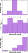 |
Fig. 2. Redshift distribution of three typical cases. The histograms show the distribution of photometric redshifts of galaxy members. Top panel: cluster candidate located within one redshift slice; the vertical line in this panel gives the mean photometric redshift value. Middle panel: flat distribution, indicating that this overdensity is not a physically connected structure. Bottom panel: distribution of a real structure, but its peak is close to the edge of our selection redshift slice, missing a large fraction of its galaxy members. |
2.2.4. Comparison with other cluster catalogues
We compare the final cluster candidate sample with several other cluster or group catalogues following different selection methods (e.g. overdensity, weak lensing, cosmic web structure). First, we compared it with the Chandra COSMOS X-ray catalogue (Gozaliasl et al. 2019). This work used extended X-ray sources detected on a 32−128 arcsec scale. The authors searched for the cluster or group members within the extended X-ray source area. And the redshift is mainly decided from spectroscopic redshift in Hasinger et al. (2018). We find three matches out of 14 clusters or groups in Gozaliasl et al. (2019). Cluster candidates 02 and 06 in our sample are matched respectively with clusters 20035 and 10052 in Gozaliasl et al. (2019) within 0.03 Mpc. Cluster candidate 11 in our sample can match with cluster 20069 in Gozaliasl et al. (2019) within 0.13 Mpc. The information of these three clusters is listed in Table 2. Apart from the three cluster candidates mentioned above, another cluster in Gozaliasl et al. (2019) was found by our method, but it does not have NIR so we do not put it in our cluster candidate catalogue; two others were selected by overdensity mapping but were ruled out due to flat photometric redshift distribution. Considering the size of the extended X-ray source is much smaller than the structure we are looking for, we also tested using the smaller 0.5 Mpc radius aperture to search for overdensities again and reproduce almost all clusters or groups in Gozaliasl et al. (2019) except the least massive one. However, these smaller size structures are more likely to be groups with low masses (< -pagination1014 M⊙) rather than clusters, so we did not use them for our analysis.
Properties of X-ray detected clusters taken from Gozaliasl et al. (2019).
Then we compared our sample with optically selected cluster catalogues. There are three matches in Bellagamba et al. (2011). In this work the clusters are selected by weak lensing data. Our cluster candidates 05, 06, and 07 match with clusters 17, 19, and 24, respectively, in their work. The information for these three clusters is listed in Table 3. Since the weak lensing method detects clusters through dark matter spatial distribution rather than through galaxy overdensities, the difference is expected.
Properties of weak lensing selected clusters from Bellagamba et al. (2011).
We also compared our cluster candidates with the COSMOS environment catalogue (Darvish et al. 2017), where the authors use photometric data from Laigle et al. (2016) to construct a density field. They identify the environment (cluster, filament, field) from the density field for each galaxy without giving cluster information. We slice the galaxy redshifts as in this work, plot cluster galaxies in each slice and compare them with our cluster candidates. Our cluster candidates (01, 02, 04, 05, 06, 07, 08, 10, 14, 15, and 17) match well with dense regions of cluster galaxy distribution. The other cluster candidates also contain cluster galaxies in the aperture, but their centres are offset from the densest regions.
In conclusion, 12 of our 17 cluster candidates have good matches with the clusters discovered in previous studies. In previous works, all 17 cluster candidates have a cluster match within 1 Mpc.
3. Methods
In Sect. 3.1 we describe how we classify RQGs, SFGs, and QGs. In Sect. 3.2 we explain how we separate fast- and slow-quenching galaxies on the UVJ diagram. In Sect. 3.3 we explain how we remove the impact of possible projection effects.
3.1. Photometric selection of RQGs
3.1.1. Rest frame colour index estimation
We used the EAZY code (Brammer et al. 2008), which fits the SED by maximising the likelihood between the observed and template predicted SED. The templates of EAZY are set purely on stellar population synthesis models, which suit deep optical-NIR surveys. A non-negative matrix factorisation (NMF) algorithm (Blanton & Roweis 2007) is adopted to reduce the number of templates while keeping the ability to reproduce observations. For input of NMF, the library of PEGASE models described in Grazian et al. (2006) is used. This library includes ∼3000 models with ages from 1 Myr to 20 Gyr and several models for SFHs. These templates also consider dust extinction using the Calzetti et al. (2000) law and include emission lines. The EAZY code fits SED using a linear combination of these templates. Through the SED fitting, rest-frame UVJ colours can also be derived. In this work, we use rest-frame U and V filter information from Maíz Apellániz (2006) and rest-frame J band from 2MASS survey (Skrutskie et al. 2006). We fix the redshifts of galaxies to the photometric redshifts estimated in the COSMOS2015 catalogue (Laigle et al. 2016). As a result, EAZY provides the interpolated colour index LX (X = U, V, J). Then the U − V and V − J colour indices are calculated from the U, V, and J colour indices with the form
 (3)
(3)
3.1.2. Rest-frame UVJ diagram
The rest-frame UVJ diagram is a common tool for separating QGs and SFGs (e.g. Daddi et al. 2004; Patel et al. 2012; Arnouts et al. 2013). QGs are redder in U − V colour for a given V − J colour, due to their strong Balmer break feature. Since RQGs are transitional galaxies between these two populations, a natural thought is that they should also reside in a region between these two populations on the rest-frame UVJ diagram.
The location of RQGs on the UVJ diagram (Fig. 3) has been discussed in many works, such as Almaini et al. (2017), Schreiber et al. (2018), Belli et al. (2019), and Wu et al. (2020). These works show the UVJ colours of RQGs selected by the principal component analysis (PCA) method (based on supercolours derived from galaxy photometry that correlates with galaxy spectral features, mainly D4000 and absorption line), the specific star formation rate (sSFR) obtained from SED fitting, Keck/MOSFIRE spectra, and LEGA-C spectra, respectively. It is noted that the boundaries between different populations are arbitrary. Taking advantage of the existing comparisons, we set our own selection boundaries to include as many RQGs as possible, while keeping a relatively low contamination level (see Sect. 5.1).
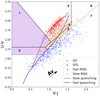 |
Fig. 3. Rest-frame UVJ diagram used to classify galaxy populations. The solid black lines are boundaries in Schreiber et al. (2018). The dashed lines are the modified boundaries used in this work (see Sect. 3.1.2). The red dots are QGs; blue dots are SFGs; purple and orange dots are both RQGs. The colour-shaded regions are RQG regions, and they are divided into fast- and slow-quenching regions. The two regions are divided by black and red diagonal solid lines according to evolution tracks (red and purple lines) of two model galaxies with a 1 and 0.1 Gyr quenching timescale, respectively (see Sect. 3.2). The arrow is the dust extinction vector corresponding to E(B − V)=0.1. Numbers indicate the different regions: 1 and 2 are fast-quenching RQG; 3 and 4 are slow-quenching RQG; 5 and 6 are QG; 7 is SFG. |
In this paragraph we briefly introduce how our boundaries are decided (Fig. 3). We modified the boundaries from Schreiber et al. (2018) (solid black lines), which separates SFGs (region 2, 3, 6, and 7) and QGs (region 1, 4, and 5). In this work dusty and non-dusty galaxies are divided by a diagonal line. We restrict it within the quiescent region to separate the post-starburst galaxies (region 1) and fully quenched QGs (region 4 and 5) as in Wild et al. (2014) and Almaini et al. (2017). However, some works (Almaini et al. 2017; Schreiber et al. 2018; Wu et al. 2020) identified RQGs outside the solid boundaries in both star-forming and quiescent regions by different methods (e.g. PCA method, SED fitting, spectral features). Therefore, we shifted the original solid horizontal boundary to U − V = 1.1 (grey dashed horizontal line) and shifted the diagonal boundary by ±Δ(U − V)=0.1 (grey dashed diagonal lines) to add regions 2, 3, and 4 into the original post-starburst region 1. The final RQG sample (regions 1, 2, 3, and 4) should fulfil all the following conditions:
 (4)
(4)
Figure 3 depicts all the boundaries used to classify these three galaxy populations. The SFGs (blue points) lie in region 7 and show a sequence depending on dust extinction. The QGs (red points) are in regions 5 and 6, and the dusty QGs are in region 6 (Almaini et al. 2017). The RQGs lie between the SFG and QG populations, in the middle of the evolutionary paths from SFGs to QGs, as shown by the solid curves (see Sect. 3.2). The RQG region (1, 2, 3, and 4) is shown with purple and orange shading. There is a concern that these arbitrary boundaries may lead to some uncertain results. However, we shift the boundaries between QG and RQG by 0.1 mag and find that it does not affect our qualitative results.
3.2. Fast- and slow-quenching galaxy separation
The quenching timescale is an important factor in understanding its physical mechanisms. To put a strict constraint on the quenching timescale, it is necessary to obtain high-resolution, high S/N rest-frame optical spectra to fit the galaxy model. However, the number of our sample galaxies with spectra is limited. To give an idea of how the quenching timescale depends on different parameters, we take a photometric approach and apply model colour tracks to separate galaxies with different quenching timescales.
The SFH model we adopt has a constant star formation period followed by an exponentially declining star formation quenching phase, as illustrated in Fig. 4. The star formation rate (SFR) evolution with age is set by Eq. (5)
 (5)
(5)
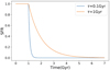 |
Fig. 4. Star formation history models with a constant star formation period followed by exponentially declining quenching period with τ = 0.1 and 1 Gyr. |
where τ is the quenching timescale.
To understand how galaxies move in the rest-frame UVJ space, we used the CIGALE code (Boquien et al. 2019) to make galaxy models and estimate their rest-frame colours. In the estimation of rest-frame UVJ colours, we used exactly the same filter as in Sect. 3.1.1. In this work we assume the galaxies have Chabrier (2003) initial mass function, solar metallicity, and Calzetti et al. (2000) dust attenuation curve with E(B − V)=0.15. Since the RQGs have some remaining star formation, there should be a certain amount of dust. And we arbitrarily choose the value of E(B − V)=0.15 for galaxies in the RQG phase. More details of the effects of dust attenuation on the evolutionary paths are discussed in Appendix A. For a fast quenching galaxy we assume a quenching timescale of 0.1 Gyr, and for a slow-quenching galaxy we assume a quenching timescale of 1 Gyr. In Appendix A we discuss how different parameters affect evolutionary pathways in the UVJ space. The evolutionary pathways of the two model galaxies are plotted in Fig. 3. We can see there is a clear difference between the fast and the slow quenching tracks. To separate the fast (purple) and slow (orange) quenching regions, we adopt two lines. For regions 1 and 4, we adopt the solid diagonal line from Schreiber et al. (2018). For regions 2 and 3, we draw a solid red line with the same slope as the previous one where the slow quenching track enters the RQG region.
CIGALE also allows us to estimate the time when the model galaxies stay in the RQG selection area, and we define this time as the visibility timescale. When the quenching timescale is 0.1, 0.3, 1, and 2 Gyr, the visibility timescale is 0.43, 0.58, 1.5, and 2.6 Gyr, respectively. Generally, galaxies with a longer quenching timescale have a longer visibility timescale. This trend will help us understand our results better. However, since the galaxy models here are simplified, the value of the visibility timescale will not be used for quantitative analysis.
3.3. Field subtraction
In order to select galaxy cluster candidates we used photometric redshifts adopting redshift intervals (full width) of Δz = 0.1 at 0.5 < z < 1. However, the intrinsic scatter of a cluster in redshift space is much smaller than Δz = 0.1. Therefore, there should be many galaxies that are not physically associated with our cluster candidates in each redshift slice. Thus, we need to apply a statistical field subtraction to correct for such a projection effect. To achieve this we first define the field regions following the same method applied during the cluster candidate search. We use aperture density maps for each redshift slice and define the field area as the regions with densities lower than the 1σ threshold, which corresponds to the regions outside the cyan contours in Fig. 1. Information of the field samples in each redshift slice is shown in Table 4.
Information of the field sample in each redshift slice.
Before performing the field subtraction, we divide our sample of cluster and field galaxies into several stellar mass bins, which will be used to carry out our environmental analysis in Sect. 4. Finally, we compute the density of each population (SFG, RQG, QG) within each stellar mass bin and subtract the field contribution from each population using the equation
 (6)
(6)
where Nsubtracted is the number of galaxies after the subtraction, N is the number of galaxies before the subtraction, Σk is the field density of each population, and Ncluster is the total number of the cluster candidates in this redshift bin. While studying the environmental dependence, galaxies are also binned in local density (Σ5) during our analysis. Thus, we need to subtract possible field galaxies from each local density bin as well. After computing the field density of each population, we then subtract it by applying
 (7)
(7)
where Σk is the field density of each population and Σfield is the field density. The first item in brackets is the probability that a cluster candidate member galaxy is a field galaxy; the second item is its probability of being an SFG, an RQG, or a QG. After calculating this probability for each cluster candidate member, we then sum up this value for all galaxies in the local density bin.
4. Results
In this section, we present the results of our analysis in our selected cluster candidate sample (Table 1). The average field densities are displayed in Table 4. All errors in this section are propagated based on the Poisson statistics for both the original data and the field subtraction using a standard method. The information of all the bins analysed in this section is listed in the tables in Appendix B.
4.1. Quenching efficiency
Galaxy quenching drives SFGs to evolve into RQGs. Thus, the ratio of these two populations can represent the efficiency of the quenching process. Hence, we define the quenching efficiency as
 (8)
(8)
Figure 5 presents how Q.E. depends on stellar mass. The left panel also shows a comparison between the cluster candidates and the general field. Q.E. shows a strong dependence on the stellar mass, especially in the most massive bin. The Q.E. is always higher in the cluster candidates, showing that the cluster candidate environment is enhancing it. The gap is much more prominent in the most massive bin, indicating that the mass quenching is also stronger in the cluster candidates. To see how the local galaxy density affects the mass-dependent quenching, we divide our sample into high- and low-density subsamples at 101.3 Mpc−2 (i.e. 20 Mpc−2), each of which contains one-half of the galaxy sample (middle and right panels in Fig. 5). It turns out that the local environment does not have a substantial impact on mass-dependent quenching, and that there is a significant rise in the Q.E. with stellar mass for both sparse and dense local environments.
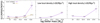 |
Fig. 5. Mass dependence of Q.E. Left panel: dependence in all environments in our sample cluster candidates. Middle and right panels: dependence in two subsamples divided by local density. The total number of galaxies in the two subsamples are the same. The number to the left of each data point is the number of RQGs in this mass bin, while the number to the right is the number of SFGs. The total number of SFGs or RQGs in the middle and the right panels is the same as the number of the cluster candidates in the left panel. Errors are propagated based on the Poisson statistics error of each population in each bin. |
In the left panel of Fig. 6 the Q.E. in the cluster candidates shows a dependence on the local density, which supports the scenario of environmental quenching. In the field the Q.E. is slightly lower than the lowest local density bin in the cluster candidates, indicating that the outskirts of the cluster candidates have a similar enhancement in galaxy quenching to that in the field. The sample is divided into low-mass and high-mass subsamples at M* = 1010.42 M⊙ for analysis. In both of these subsamples, Q.E. increases with local density. However, considering the errorbars, we can only say that the environmental dependence in low-mass systems (the middle panel of Fig. 6) is significant. If we compare the Q.E. in the two subsamples, high-mass galaxies have higher Q.E., which again confirms the presence of mass-dependent quenching.
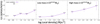 |
Fig. 6. Environmental dependence of Q.E. Left panel: dependence of all masses. Middle and right panels: dependence in two subsamples divided by stellar mass. The total number of galaxies in the two subsamples are the same. The number to the left of each data point is number of RQGs in this mass bin, while the number to the right is the number of SFGs. The total number of SFGs or RQGs in the middle and the right panels is the same as the number of the cluster candidates in the left panel. Errors are propagated based on the Poisson statistics for each population in each bin. |
4.2. Quenching stage
When the quenching process is finished, RQGs become QGs. Therefore, we define quenching stage as the number ratio of these two populations
 (9)
(9)
where the Q.S. value indicates how much the quenching process has proceeded for a given galaxy sample. When the Q.S. value is high, many galaxies are in the RQG phase and are undergoing quenching, indicating a relatively early stage of quenching. On the other hand, if the Q.S. value is low, it means that most of the galaxies are already quenched and have become old QGs.
As can be seen in the left panel of Fig. 7, the Q.S. decreases with stellar mass, especially for the least massive bin. The Q.S. in the field is higher than in the cluster candidates, showing they are in an earlier phase of quenching. The lowest mass galaxies are at an earlier stage of quenching, which is consistent with the downsizing scenario in which massive galaxies form and quench earlier than low-mass ones.
 |
Fig. 7. Mass dependence of Q.S. Left panel: dependence in all environments in our sample of cluster candidates. Middle and right panels: dependence in two subsamples divided by local density (same bin division as in Fig. 5). The number to the left of each data point is the number of RQGs in this mass bin, while the number to the right is the number of QGs. The total number of QGs or RQGs in the middle and right panels is the same as the number of cluster candidates in the left panel. Errors are propagated based on the Poisson statistics for each population in each bin. |
We then try to reveal how the local environment affects this relation (Fig. 7, centre and right diagrams). The full sample was divided into a high and a low local density subsample using Σ5 at 20 Mpc−2 as a threshold, and ensuring that each subsample contains half of all the galaxies. The trend between the Q.S. and stellar mass is only significant for the denser local environment. As in Fig. 8, the Q.S. clearly decreases with local density. If we separate massive and less massive subsamples at M* = 1010.42 M⊙ (Fig. 8), the trends are still seen in both subsamples, but are less significant due to decreased sample sizes. The Q.S. in the field is lower than the least dense cluster bin. However, the current field sample size is large, and the errorbar will increase if it has a similar size to that in the cluster. Therefore, this result is not significant and we do not discuss it further here. We also note that mass dependence shows different properties in two local density bins, and environment dependence shows different values in two mass bins. Hence, the mass dependence of quenching also has a dependence on the environment, and the environment dependence of quenching also has a dependence on stellar mass.
 |
Fig. 8. Environmental dependence of Q.S. Left panel: dependence for all environments. Middle and right panels: dependence in different mass bins (same bin division as in Fig. 6). The number to the left of each data point is the number of RQGs in this density bin, while the number to the right is the number of QGs. The total number of QGs or RQGs in the middle and the right panels is the same as the number of cluster candidates in the left panel. Errors are propagated based on the Poisson statistics for each population in each bin. |
4.3. Quenching timescale
4.3.1. Mass, environment, and redshift dependence
As we have emphasised, the quenching timescale is an important factor for discriminating among the different physical mechanisms of quenching. Although we separate fast- and slow-quenching galaxies only based on the rest-frame UVJ diagram, we can still use the number ratio of these two populations to illustrate the qualitative dependence of the quenching timescale on mass and environment.
In Fig. 9 we show that the number ratio of slow-quenching galaxies over fast-quenching galaxies increases with the stellar mass, which means that low-mass galaxies have shorter quenching timescales compared to those of massive galaxies. This suggests that the quenching of galaxies with different stellar mass is dominated by different physical mechanisms.
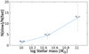 |
Fig. 9. Quenching timescale increase with stellar mass. The number to the left and right of each data point respectively show the number of slow- and fast-quenching galaxies for each mass bin. Errors are derived based on the Poisson statistics for each population in each bin. |
In Fig. 10 there is a possible dependence of the quenching timescale on the local density. The ratio seems to have a peak in the intermediate density bin with large uncertainty. However, we cannot say whether it is related to any physical trend since our sample size is still limited.
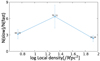 |
Fig. 10. Quenching timescale does not have a clear relation with local density. The number to the left and right of each data point respectively represent the number of slow- and fast-quenching galaxies for each mass bin. Errors are derived based on the Poisson statistics error of each population in each bin. |
Figure 11 shows a clear trend that fast quenching is more important at higher redshifts. This suggests that the main quenching mechanism changes with redshift, and the short timescale quenching becomes more important at higher redshifts, which is consistent with the results in Cucciati et al. (2012) and Rowlands et al. (2018).
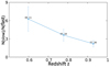 |
Fig. 11. Quenching timescale decrease with redshift. The number to the left and right of each data point respectively represent the number of slow- and fast-quenching galaxies for each mass bin. Errors are derived based on the Poisson statistics error of each population in each bin. |
4.3.2. Two specific cases
Here we highlight two specified cases in quenching that show the largest difference in the slow and fast quenching ratio. These cases probably correspond most directly to the mass and environment-dependent quenching, respectively.
In Table 5 the first case is the quenching of massive galaxies in a low-density environment. High mass refers to the higher 50% of mass (i.e. > 1010.42 M⊙). Low local density refers to the lower 50% of local density (i.e. < 101.3 Mpc−2). This case should be mainly affected by mass-dependent quenching. The N(slow)/N(fast) ratio has a high value, giving a hint that the mechanism working in this case has a long timescale. This is likely to be, for example, AGN feedback, given that AGNs are exclusively hosted by massive galaxies, and the AGN feedback can be a slow quenching process with a timescale of a few Gyr (Hirschmann et al. 2017).
N(slow)/N(fast) values and their errors in the two specified cases.
The second case is the quenching of low-mass galaxies in a dense environment, which is expected to be more affected by the environment. The N(slow)/N(fast) ratio is much lower compared to the first case, showing the impact of a short timescale mechanism. It is likely to be, for example, ram pressure stripping, which strips gas from low-mass galaxies more easily due to their shallow gravitational wells. Moreover, ram pressure stripping can only occur in dense cluster cores on a relatively short timescale (Steinhauser et al. 2016). However, short timescale AGN feedback quenchings also exist, and they can play a role in this case as well.
We note that we cannot reject other possibilities since the information we are able to obtain with photometric data alone is still limited.
4.4. Visibility timescale
In addition to the reasons we analysed in the previous sections, we should note that the visibility timescale of galaxies can also play a role in our results. The visibility timescale is a galaxy’s timescale of staying in the RQG region on the UVJ diagram. If the visibility timescale also depends on stellar mass or local density, it would degenerate with the Q.E. and Q.S. In Sect. 3.2 we show that galaxies with longer quenching timescales generally spend a longer time in the RQG region on the UVJ diagram. However, with photometric data solely, we cannot constrain the visibility time with a small enough uncertainty to completely break the degeneracy between the mass and environment dependence of the visibility time and quenching properties. Hence we only separate the fast quenching (short visibility time) and the slow quenching (long visibility time) bins, and estimate their contributions to determine how the visibility timescale affects our results.
In Fig. 12, we show how the fast-quenching (short visibility time) galaxies and the slow-quenching (long visibility time) galaxies contribute to the mass and the environment dependence of Q.E. and Q.S. In the mass dependence of the Q.E. panel (top left panel), we can see that the long visibility time galaxies have a strong mass dependence, while the short visibility time galaxies do not. The figure shows that the visibility time affects the Q.E.; the increasing trend of Q.E. is partly due to the mass dependence of visibility time, and the massive galaxies tend to stay in the RQG region for more time. In the local density dependence of the Q.E. panel (top right panel), both fast- and slow-quenching galaxies show an increasing trend, indicating that the visibility time does not have a strong impact on the environment dependence of Q.E. This is consistent with Sect. 4.3, where we show that the quenching timescale has a dependence on the stellar mass but not on the local density. In the Q.S. panels (bottom two panels), both fast- and slow-quenching galaxies show a decreasing trend (similar to the overall trend), showing that the visibility time does not strongly degenerate with the mass or environment dependence of the Q.S.
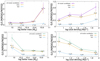 |
Fig. 12. In this figure, we show results of Q.E. and Q.S. in fast- and slow-quenching galaxies separately. Slow-quenching galaxies (same as long visibility timescale galaxies) are marked with orange points, while fast-quenching galaxies (same as short visibility timescale galaxies) are marked with light blue points. |
In Sect. 4.3.1 the degeneracy between the quenching timescale and visibility timescale exists as well. However, there is no proper way to break this degeneracy with only galaxy photometry. We should keep this degeneracy in mind when interpreting the physical scenario of quenching.
In conclusion, while analysing the mass dependence of Q.E., we should be careful of the influence of RQG visibility time. We leave this issue to our future work. When we have the spectra of RQGs, we can disentangle the degeneracy between the quenching properties and the visibility time.
4.5. RQG comoving number density
As mentioned in Sect. 3.3, the RQGs, fast-quenching RQGs, and slow-quenching RQGs all show relations with redshift. To better understand this dependence, we calculated the comoving number densities in each redshift bin. In this section not only do we use the galaxies in our 17 cluster candidates, but also all the galaxies in the COSMOS field with M* > 1010 M⊙.
In Fig. 13 we present the number densities of fast-quenching galaxies, slow-quenching RQGs, and total RQG sample in different redshift bins (including both field and cluster candidate regions). We bin all galaxies into two groups to increase the statistics. The low-z bin range is 0.5 < z < 0.75, while the high-z bin refers to 0.75 < z < 1.0. Both slow- and fast-quenching RQGs show an increasing trend with redshift, and the fast-quenching RQGs show a steeper slope. The increasing trend of fast-quenching RQGs is consistent with Belli et al. (2019) and Wild et al. (2016) who reveal that the number density of post-starburst galaxies (corresponding to fast-quenching RQGs in this work) increases with redshift. Comparing the slope of slow- and fast-quenching galaxies, we can tell that, similar to the trend in cluster candidate regions, fast quenching is more important at higher redshifts (see Sect. 4.3.1).
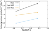 |
Fig. 13. Comoving number density evolution of all RQGs, slow-quenching RQGs, and fast-quenching RQGs. To increase the statistics, all galaxies are put into two bins, 0.5 < z < 0.75 (low redshift) and 0.75 < z < 1.0 (high redshift), consisting of 1468 and 2419 RQGs, respectively. |
5. Discussions
In Sect. 5.1 we discuss the contamination and completeness of our photometric RQG selection method. In Sect. 5.2 we discuss the physical implications of our results.
5.1. Spectroscopic confirmation of our RQG selection
Our current result is based on photometric data. However, the UVJ selection is not fully confirmed by galaxy spectra, while the only way to precisely determine a galaxy’s RQG properties is through its spectral features. The main limitation of RQG research is that it is a rare population, making it expensive to obtain a large sample of RQG spectra. Fortunately, the COSMOS field already has deep spectroscopic data available for many galaxies, enabling us to match our targets with the existing spectra.
We use spectroscopic data from DEIMOS 10K spectroscopic survey catalogue (Hasinger et al. 2018) and LEGA-C survey data release 3 (van der Wel et al. 2021). The DEIMOS 10K survey obtained the spectra of some of the COSMOS2015 catalogue galaxies. Depending on the galaxy, the spectral resolution can be either R ∼ 2000 or ∼2700, which are both large enough to measure the equivalent width of absorption lines. The LEGA-C survey obtained galaxy spectra with R = 2500. The parent sample LEGA-C adopts for observation is the UltraVISTA catalogue presented in Muzzin et al. (2013).
The spectral features characteristic of RQGs are strong Balmer absorption lines (Couch & Sharples 1987). We measure the galaxies’ Hδ absorption line equivalent width (EW), representing the Balmer absorption. For all the galaxies within our sample, galaxies with other strong Balmer absorption lines (e.g. Hγ, Hβ absorption line) have strong Hδ absorption lines as well. Another feature of RQGs is that their star formation activities are at a low level, so we use [OII] emission line strength to examine the existence or absence of star formation activity in the galaxy in this study. We define a galaxy with EW(Hδ) < −4 Å and EW([OII]) < 5 Å (negative value represents absorption) as an RQG galaxy in this section.
The equivalent width of each line feature is calculated using
 (10)
(10)
together with Lick spectral indices (Salaris & Cassisi 2005) and the index of the [OII] line from Balogh et al. (1999). Here FI, λ is the index flux, which is obtained from the index band; FC, λ is the continuum flux, which we assume to be constant over the index band. The continuum flux is calculated from the average flux over blue and red continuum bands. We do not remove the infilling emission in the calculation of EW(Hδ). All the spectral index information is listed in Table 6.
Spectral indices of RQG feature lines used in this study.
For the DEIMOS 10K observations, in addition to matching our RQG sample with their spectroscopic catalogue, we also checked the spectra they labelled with the Hδ line feature. We have 105 matches in the DEIMOS 10K catalogue. For the LEGA-C survey, we only matched our RQG sample with their catalogue. We matched the target positions within 1″, and we find 23 matched RQGs. However, we find that there are spectra in both surveys that cannot provide a high enough S/N for accurate absorption line EW measurement, for which there are various reasons. In particular, the DEIMOS 10K spectra mostly have exposure times from 1 to 3 h, which is not long enough for less luminous galaxies. To avoid contamination from poor-quality spectra, we select galaxies with EW errors of all four measured spectral lines σi < 0.8 Å (i = Hδ, [OII]). This error cut leaves us with 40 high-quality spectra (28 from DEIMOS 10K and 12 from LEGA-C). Another thing we should note is that the DEIMOS spectrograph has two chips that produces an artificial break in the spectrum at around 7600 Å. To avoid this effect, we checked all good-quality spectra and remove those with this break in either the continuum or the index band of any of the four lines. There are RQG spectra without Hδ coverage in both DEIMOS 10K and LEGA-C, and we remove these galaxies as well. In total, we are left with 27 UVJ-selected RQGs with good enough spectra for spectroscopic confirmation. Their information is listed in Appendix C.
The positions of these 27 galaxies on the UVJ diagram are plotted in Fig. 14. Among the 27 RQGs, 14 galaxies have strong Balmer absorption lines (EW(Hδ) < −4 Å). For the 13 galaxies below this threshold, we checked their colour index errorbars on the UVJ diagram (red marks in Fig. 14). Based on the fluxes and errors given in the COSMOS2015 catalogue, we randomly generate 1000 flux values following Gaussian distribution and then calculate rest-frame colour indices from these fluxes. In this way we can calculate the 3σ errors for all galaxies. Nine galaxies out of 13 are close to the boundary. We also cross-matched these 13 galaxies with Chandra COSMOS Legacy Survey data (Civano et al. 2016), and found two galaxies with Hδ emission lines (ID 908883 and 635561) are X-ray AGNs. We should also note that all these galaxies with weak Balmer absorption features lie in the slow-quenching region, which confirms that the quenching timescale of this UVJ region is longer, that their stellar populations have already grown old, and thus that the Balmer absorption feature has started to fade. Six of the 13 galaxies (ID 314012, 375916, 391497, 438059, 559691, 810957, 816426, and 837551) have −4 Å < EW(Hδ) < −1.5 Å; meanwhile, their spectra are passive. This is consistent with what we discuss in Fig. A.2. In Fig. A.2 we show the evolution of EW along the evolutionary paths of model galaxies. The galaxies in slow-quenching regions show weak Hδ absorption lines (as weak as EW(Hδ) ∼ 1.5 Å). The remaining three galaxies are possible contamination. Therefore, we conclude that the overall contamination rate is not high.
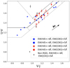 |
Fig. 14. UVJ-selected RQGs with strong absorption lines (in blue) and without strong absorption lines (in red) and their rest-frame UVJ colour uncertainties. Star symbols are galaxies without strong [OII] emission, while squares are galaxies with strong [OII] emission lines. Crosses are galaxies that are not selected as RQG in the UVJ diagram, but with RQG spectral features and their UVJ colour uncertainties. The arrow shows the reddening vector. |
However, in the 14 strong absorption line galaxies, 8 (6 of which are slow-quenching galaxies) also have strong [OII] lines (EW([OII]) > 5 Å). This is consistent with the work of Rudnick et al. (2017), who find [OII] emission in quenched galaxies. The [OII] emission may indicate that the depletion time is indeed longer for slow-quenching galaxies, keeping the galaxy forming stars for a long time. However, we still need further work to fully understand the source of [OII] in RQGs. In Fig. 15, we present typical examples of one strong and one weak absorption galaxy spectra.
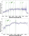 |
Fig. 15. Two checked galaxy spectra (in observed frame). Spectral features are indicated with green dashed lines. An artificial break between two chips of the DEIMOS spectrograph is shown as a grey shaded area. Top panel: typical spectrum for strong Balmer absorption line galaxy, at z = 0.864. Bottom panel: typical spectrum for weak Balmer absorption line galaxy, at z = 0.553. |
In addition to the RQGs, we found two QGs and two SFGs that satisfy the RQG criteria in all high-quality spectra (Fig. 14). Their information is listed in Appendix C. The SFG at the bottom (ID 897743) has clear AGN features (i.e. a broad MgII emission line, broad Hγ and Hβ emission lines). The other SFG and one of the QGs are near the RQG region boundaries. However, for the other QG, which is far away from any boundary, we may have a risk of missing a certain subpopulation of RQGs that, for some reason (e.g. undergoing stronger starburst before quenching) spend more time in the recently quenched phase.
In conclusion, our photometric UVJ selection method still suffers from certain contamination and completeness problems, but judging from the current spectroscopic data, neither the contamination nor the incompleteness is high. Hence, our results from photometric data are still trustworthy. Due to the lack of high-quality spectra for absorption measurements, we do not have a statistical sample to estimate a reliable contamination or completeness rate. Deeper and wider spectroscopic observations of RQGs are required to better assess our photometric method.
5.2. Physical scenarios of quenching processes
In Sect. 4.1 we show that the Q.E. increases with both the stellar mass and the local density. From the Q.E., we can see that the mass dependence trend is not greatly affected by the local density, but the efficiency is higher in denser local environments, especially in the highest local density bin. It shows that mass quenching happens in all kinds of environments, but the cluster environment (i.e. dense environment) can also enhance the quenching of massive galaxies. The most significant increase in efficiency appears in the most massive bin, indicating that mass-dependent quenching is much stronger for the massive galaxies. The Q.E.’s dependence on local density is not independent. It is also affected by the stellar mass, so that for massive galaxies, this dependence almost disappears (see the middle and right panels of Fig. 6). Therefore, although the environmental effects of quenching also exist, they are only efficient in affecting low-mass systems. Our definition of Q.E. is different from commonly used definitions based on the fraction of QGs (e.g. Kawinwanichakij et al. 2017; van der Burg et al. 2020; Reeves et al. 2021). Since our definition introduces the RQG population, which may still be in the process of quenching, it can convey the efficiency more directly. In Kawinwanichakij et al. (2017) the authors separate mass-dependent quenching efficiency and environmental quenching efficiency. To compare our result with theirs, we also calculated our mass quenching efficiency using their definition (see Eq. (5) in Kawinwanichakij et al. 2017). In Kawinwanichakij et al. (2017) the mass-dependent quenching efficiency increases with stellar mass; the trend is consistent with our result. In the least massive bin our quenching efficiency is ∼0.3 dex higher, and in other bins our efficiencies are ∼0.1 dex higher than the Kawinwanichakij et al. (2017) result. This might be due to different sample completeness or cosmic variance of our data. The environmental quenching efficiency in Kawinwanichakij et al. (2017) does not show a significant evolution with stellar mass. In our work we only use two stellar mass bins while discussing environmental quenching, but instead we discuss its dependence on local density. In general, low-mass galaxies in our sample have lower efficiency, but this strongly depends on local density. We note that in Kawinwanichakij et al. (2017) the efficiency at the massive end has extremely large errorbars, and therefore we cannot establish a reliable comparison in that mass range. In van der Burg et al. (2020) the authors discuss quenching efficiency as a function of stellar mass; the resulting trends and binned values both agree with our result. In Reeves et al. (2021) the authors discussed how the quiescent galaxy fraction depends on stellar mass. The trends they found agree with our results, except in the least massive bin where our quiescent galaxy value is slightly higher than theirs. This is likely a consequence of the different redshift range studied in their analysis (1.0 < z < 1.5). At that redshift low-mass galaxies are predominantly not quenched, hence their fraction is lower. The authors also pointed out that the environment and mass dependence of quenching are not separable, which is consistent with our result. McNab et al. (2021) studied the mass dependence of quenching by the excess of cluster SFG fraction over the field SFG fraction. The increasing trend of the excess represented by quenching efficiency agrees with our result. Webb et al. (2020) studied the SFR declination rate in field and cluster galaxies by spectroscopy and photometry fitting. Their results show that cluster galaxies (i.e. denser environment galaxies) quench faster, which also agrees with our results.
In Sect. 4.2 we see that the Q.S. decreases with both the stellar mass and the local density. The Q.S. provides us with a glimpse of quenching in the past. It significantly decreases with stellar mass at the low-mass end (similarly for the cluster candidates and the field), showing that more massive galaxies are at a much later stage of quenching. This is consistent with the downsizing scenario (e.g. Cowie et al. 1996; Cattaneo et al. 2008; Webb et al. 2020) that massive galaxies form and quench earlier, and hence they are at a later, more advanced stage of evolution compared to low-mass galaxies. The mass dependence of the quenching stage is strongly affected by the local density. The trend is only significant in high-density environments. For sparse environments, the errorbars are too large for us to say anything. The scenario is consistent with Hatch et al. (2011), where faster evolution in protoclusters is found. This can also be due to the migration of galaxies from the low-density cluster outskirts to the high-density cluster cores where the quenching happens. The Q.S. also shows a stable decreasing trend with the local density, indicating that galaxies in denser environments (cluster cores) are at a later, more advanced stage of quenching. The earlier Q.S. of field galaxies also supports this scenario. This is consistent with the inside-out quenching in clusters, where galaxies in cluster cores quench early, while the galaxies in the outer parts quench progressively later, which is consistent with the scenario in Koyama et al. (2013) and Shimakawa et al. (2018). Another possibility is that during the in-falling process their gas will be stripped off, which directly leads to their quenching (Bekki et al. 2002). In this case the effect should be stronger for low-mass galaxies since their gas components are easier to strip. This environmental dependence is not strongly affected by the stellar mass, which supports the inside-out quenching that has an impact on low- and high-mass galaxies equally. In McNab et al. (2021) the authors use three types of transitional populations: green valley (GV) selected by rest-frame (NUV−V) and (V − J) colours; blue quiescent (BQ) selected by rest-frame (U − V) and (V − J) colours; and post-starburst (PSB) selected by galaxy spectra. They connect the quenching timescale to the transitional population fraction excess in clusters. They found that the lowest mass systems (< 1010.5 M⊙) have short quenching timescales (< 1 Gyr), which agrees with our result that low-mass galaxies are dominated by fast quenching (< 1 Gyr).
The slow-to-fast quenching ratio is an indicator of the quenching timescale. In Sect. 4.3 we find that the massive galaxies are dominated by slow-quenching, and the less massive galaxies are dominated by fast quenching. This result is consistent with Walters et al. (2022), where the authors find that slow quenchers tend to have higher stellar mass. The authors used IllustrisTNG simulation (Nelson et al. 2019) to estimate the quenching timescale. Walters et al. (2022) also used MaNGA IFU survey data (Bundy et al. 2015) and took measurements of the stellar age gradient from Woo & Ellison (2019) to split fast and slow quenchers. In this way the authors confirmed that slow quenchers have higher stellar mass. In Hahn et al. (2017) the authors matched N-body simulation from Wetzel et al. (2013) and their evolutionary model with SDSS DR7 Abazajian et al. (2009) data to investigate and constrain the quenching timescale. They find that satellite galaxies have shorter quenching timescales than the central ones. This result broadly agrees with this work, assuming that satellite galaxies are less massive compared to central galaxies. However, we note that the aperture we use for cluster member galaxy selection in this work is about a factor of 2 larger than R200 in our clusters (see Table 2 and R200 in Table 2 of Gozaliasl et al. 2019). Therefore, we cannot exclude the possibility that some galaxies far from the cluster centre could also be considered central galaxies of smaller haloes infalling towards the main cluster core.
In Sect. 4.3.2 two specified cases are discussed. These two cases show clearly different timescales of quenching. The mass-dependent quenching in sparse regions should be less affected by the environment. It turned out to have a longer timescale, and very likely to be AGN feedback that caused quenching. This is consistent with the observed timescale of quenching for this process (Hopkins et al. 2006) and with the typical stellar mass of host galaxies (Kauffmann et al. 2003). AGN feedback also plays an indirect role in the morphology transformation by suppressing in situ star formation, and AGN feedback is essential for forming ellipticals (Dubois et al. 2016). This could also explain the bimodality in galaxy morphology. The environmental quenching is only significant for low-mass galaxies, and it is surely stronger in denser regions. Quenching, in this case, appears to be a short timescale type, which we reasonably speculate to be caused by ram pressure stripping. As mentioned in Sect. 2.2.4, three cluster candidates are detected in X-rays, and their total masses are measured, which indicates that they are massive enough to allow ram pressure stripping to happen.
In Sects. 4.3 and 4.5 we performed a preliminary exploration of the quenching’s dependence on redshift. In both cluster candidates and the general field, the fast-quenching RQGs increase with redshift. In cluster candidates the ratio of slow-quenching RQG to fast-quenching RQG decreases with redshift, indicating that fast quenching becomes more important at higher redshift. In Tinker & Wetzel (2010), Balogh et al. (2016), Fossati et al. (2017), and Foltz et al. (2018), the authors discussed the galaxy quenching timescale’s dependence on redshift in clusters and groups. Combining their results, the quenching timescale also decreases with redshift. We estimated the comoving number density of fast-quenching and slow-quenching RQGs in the field. Fast-quenching RQGs show a strong increasing trend. This trend is consistent with the post-starburst analysis in Wild et al. (2016) and Belli et al. (2019). The redshift range they investigate is wider than ours, but both show that the number density of post-starburst galaxies increases with redshift up to z ∼ 2. Wild et al. (2016) analyses the PSBs in the UKIDSS UDS field. To compare the two sets of results, we use the PSB catalogue from Wilkinson et al. (2021) that includes PSBs from the COSMOS field. To make a direct comparison, we limit our RQG sample to the traditional PSB region in Wild et al. (2014) (region 1 in Fig. 3). We also apply the same mass cut for both samples. Then we compare the comoving number density of two samples in Fig. 16. The increasing trend is found in both samples, while the absolute value has ∼0.4 dex difference, especially in higher redshift bins. We note that Fig. 1 in Wilkinson et al. (2021) shows a spectroscopic confirmation of their PSB sample, where a large fraction of PSBs are missed by their PCA selection. The incompleteness of PCA selection may lead to the difference between the two samples.
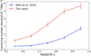 |
Fig. 16. Comparison between comoving number density of this work (RQG in traditional UVJ selection region) and Wilkinson et al. (2021) (PSB) in the COSMOS field. The five redshift bins in this plot are 0.5−0.6, 0.6−0.7, 0.7−0.8, 0.8−0.9, and 0.9−1.0. |
In this work, slow-quenching RQGs also show an increasing trend, although it is much weaker. This indicates that fast quenching processes become more important at higher redshifts. At lower redshifts, pre-processing, which is also a long timescale mechanism (Taranu et al. 2014), may be an additional quenching mechanism. This may not be as common at high redshifts because not many dense groups would exist. Therefore, the growing influence of pre-processing can result in the rising importance of slow quenching at lower redshift.
In conclusion, our photometric selection method is also a powerful tool in determining target galaxies for large systematic spectroscopic surveys of RQGs. As we apply this method to COSMOS galaxies in cluster candidates at 0.5 < z < 1.0, we obtain results with high consistency with previous works. However, our statistical analysis still suffers from the limited sample size and the uncertainty introduced by the photometric selection. We plan to increase our sample by including all Hyper Suprime-Cam Subaru Strategic Program (HSC-SSP) DEEP fields (Aihara et al. 2019). If we include IRAC data, we can also expand our sample redshift range from the current 0.5−1.0 to 0.5−2.0, which traces the quenching process back to the cosmic noon. More importantly, spectroscopic confirmation of our sample’s RQG features is required for further analysis. The preliminary spectroscopic confirmation shows low contamination and high completeness, but more spectra are required for more accurate confirmation. The high accuracy contamination and completeness rates of our UVJ selection method must be estimated and corrected to get the final results. Moreover, RQG galaxy spectra can be used to constrain quenching timescales through the spectral fitting. In this way, we can better distinguish between different mechanisms. We look forward to the Prime Focus Spectrograph (PFS; Tamura et al. 2018) on Subaru that will come into use in 2023, when we can efficiently obtain the spectra of a large sample of RQGs due to the PFS’s large field of view (1.3 deg2) and great multiplicity (2400 fibres).
6. Conclusions
In this study we constructed a multiband photometric sample of galaxies from 17 cluster candidates in the COSMOS field at 0.5 < z < 1.0. We then adopted the rest-frame UVJ selection method to classify RQGs, SFGs, and QGs. Moreover, we apply two exponentially declining SFH models with different quenching timescales to separate fast-quenching and slow-quenching galaxies on the UVJ diagram. We then correct for the projection effects introduced by the uncertainties of photometric redshifts and investigate different quenching scenarios as a function of stellar mass and local density. The main results of this study are summarised as follows:
-
We define Q.E. as the ratio of the number of RQGs to SFGs in a given volume. Q.E. increases with both mass and local density, confirming the existence of mass and environment-dependent quenching. Mass-dependent quenching is stronger for high-mass galaxies.
-
We define the Q.S. as the ratio of RQGs to QGs, aiming to quantify the history of quenching in a given volume. We find that this parameter also depends on both mass and local density. Massive galaxies are at a later stage of the quenching process, which is consistent with the downsizing scenario. Galaxies in the cluster core regions are at an earlier stage of quenching, which is a sign of inside-out quenching in cluster environments.
-
We compare the Q.E. and Q.S. of cluster and field galaxies. We find that mass quenching is enhanced by the cluster environment, and the field galaxies are at an earlier Q.S. compared to the cluster galaxies of the same stellar mass.
-
The ratio of the number of slow- to fast-quenching galaxies is a proxy of the quenching timescale. In cluster environments the quenching timescale depends both on the stellar mass and on the redshift. Low-mass galaxies are dominated by fast quenching, while massive galaxies are dominated by slow quenching. Slow quenching is also more important at lower redshifts.
-
The quenching of massive galaxies in the sparse environment is dominated by the slow quenching process. This is likely due to the relatively long timescale of AGN feedback, as AGNs are hosted exclusively by massive galaxies.
-
Fast quenching is much more important to quench low-mass galaxies in the dense environment. We believe this is likely caused by short timescale processes such as ram pressure stripping, which only happens close to the cluster core (i.e. high-density environments) and affects low-mass galaxies more efficiently.
-
Visibility time of RQGs may degenerate with the quenching properties, especially with Q.E. and timescale. However, we cannot separate well the visibility time and the quenching properties without spectroscopic data. We leave this problem for our future spectroscopic work.
-
Existing spectroscopic data confirms that our photometry-based UVJ selection method is reliable enough. By measuring the EW of Balmer absorption lines and the [OII] emission line from DEIMOS 10K spectroscopic survey data, we can confirm the RQG nature of a limited number of galaxies with high-quality spectra. Although seven UVJ-selected RQGs do not show expected strong absorption lines, two of them are AGN host galaxies and four of them lie within the slow-quenching RQG region and show relatively weak absorption lines. Thus, only one of the 17 galaxies cannot be explained, and is likely contamination. Moreover, only three galaxies outside the RQG regions have RQG spectral features, and two of them are very close to the selection boundary. Combining all these pieces of evidence, the UVJ selection method is a powerful and reliable analysis tool to investigate the RQG population before more spectroscopic data become available.
The results we present in this work give evidence of both mass-dependent quenching and environmental quenching. They also shed light on the mass and environmental dependence of quenching timescales. With future spectroscopic data the physical properties of our sample galaxies can be better constrained, and the uncertainty of current photometric results can be reduced. The UVJ selection method we displayed in this paper can be applied to large photometric datasets (e.g. HSC-SSP data) of optical to NIR. We can efficiently select RQG candidates for further spectroscopic surveys performed by high-multiplicity multiobject instruments such as PFS.
Acknowledgments
We thank the anonymous referee for his/her helpful comments, which contributed to improving the paper. We thank Drs. Omar Almaini and Sirio Belli for helpful discussions. We also thank Dr. Omar Almaini and his colleagues for kindly sharing PSB catalogue in COSMOS field selected by PCA method. T.K. acknowledge the financial support by JSPS Kakenhi (#18H03717). Two of us (ZM, NY) acknowledge support from GP-PU at Tohoku University and JST, the establishment of university fellowships towards the creation of science technology innovation, Grant Number JPMJFS2102.
References
- Abazajian, K. N., Adelman-McCarthy, J. K., Agüeros, M. A., et al. 2009, ApJS, 182, 543 [Google Scholar]
- Aihara, H., AlSayyad, Y., Ando, M., et al. 2019, PASJ, 71, 114 [Google Scholar]
- Allen, C. W. 1976, Astrophysical Quantities (London: Athlone) [Google Scholar]
- Almaini, O., Wild, V., Maltby, D. T., et al. 2017, MNRAS, 472, 1401 [NASA ADS] [CrossRef] [Google Scholar]
- Arnouts, S., Moscardini, L., Vanzella, E., et al. 2002, MNRAS, 329, 355 [Google Scholar]
- Arnouts, S., Le Floc’h, E., Chevallard, J., et al. 2013, A&A, 558, A67 [NASA ADS] [CrossRef] [EDP Sciences] [Google Scholar]
- Balogh, M. L., Morris, S. L., Yee, H. K. C., Carlberg, R. G., & Ellingson, E. 1999, ApJ, 527, 54 [Google Scholar]
- Balogh, M. L., Navarro, J. F., & Morris, S. L. 2000, ApJ, 540, 113 [Google Scholar]
- Balogh, M. L., McGee, S. L., Mok, A., et al. 2016, MNRAS, 456, 4364 [NASA ADS] [CrossRef] [Google Scholar]
- Balogh, M. L., Gilbank, D. G., Muzzin, A., et al. 2017, MNRAS, 470, 4168 [NASA ADS] [CrossRef] [Google Scholar]
- Beckmann, R. S., Devriendt, J., Slyz, A., et al. 2017, MNRAS, 472, 949 [NASA ADS] [CrossRef] [Google Scholar]
- Bekki, K. 2009, MNRAS, 399, 2221 [Google Scholar]
- Bekki, K., Couch, W. J., & Shioya, Y. 2002, ApJ, 577, 651 [Google Scholar]
- Bellagamba, F., Maturi, M., Hamana, T., et al. 2011, MNRAS, 413, 1145 [NASA ADS] [CrossRef] [Google Scholar]
- Belli, S., Newman, A. B., & Ellis, R. S. 2019, ApJ, 874, 17 [Google Scholar]
- Belli, S., Contursi, A., Genzel, R., et al. 2021, ApJ, 909, L11 [NASA ADS] [CrossRef] [Google Scholar]
- Best, P. N., Kauffmann, G., Heckman, T. M., et al. 2005, MNRAS, 362, 25 [Google Scholar]
- Blanton, M. R., & Roweis, S. 2007, AJ, 133, 734 [NASA ADS] [CrossRef] [Google Scholar]
- Boquien, M., Burgarella, D., Roehlly, Y., et al. 2019, A&A, 622, A103 [NASA ADS] [CrossRef] [EDP Sciences] [Google Scholar]
- Boselli, A., & Gavazzi, G. 2006, PASP, 118, 517 [Google Scholar]
- Brammer, G. B., van Dokkum, P. G., & Coppi, P. 2008, ApJ, 686, 1503 [Google Scholar]
- Bruzual, G., & Charlot, S. 2003, MNRAS, 344, 1000 [NASA ADS] [CrossRef] [Google Scholar]
- Bundy, K., Bershady, M. A., Law, D. R., et al. 2015, ApJ, 798, 7 [Google Scholar]
- Burgarella, D., Buat, V., Gruppioni, C., et al. 2013, A&A, 554, A70 [NASA ADS] [CrossRef] [EDP Sciences] [Google Scholar]
- Calzetti, D., Armus, L., Bohlin, R. C., et al. 2000, ApJ, 533, 682 [NASA ADS] [CrossRef] [Google Scholar]
- Capak, P. 2016, The Early Growth of Galaxies: The HST, Spitzer and Herschel Joint Legacy, 6 [Google Scholar]
- Capak, P., Aussel, H., Ajiki, M., et al. 2007, ApJS, 172, 99 [Google Scholar]
- Cattaneo, A., Dekel, A., Faber, S. M., & Guiderdoni, B. 2008, MNRAS, 389, 567 [NASA ADS] [CrossRef] [Google Scholar]
- Ceverino, D., & Klypin, A. 2009, ApJ, 695, 292 [Google Scholar]
- Chabrier, G. 2003, PASP, 115, 763 [Google Scholar]
- Chiang, Y.-K., Overzier, R., & Gebhardt, K. 2013, ApJ, 779, 127 [Google Scholar]
- Civano, F., Marchesi, S., Comastri, A., et al. 2016, ApJ, 819, 62 [Google Scholar]
- Combes, F. 2017, Front. Astron. Space Sci., 4, 10 [NASA ADS] [CrossRef] [Google Scholar]
- Couch, W. J., & Sharples, R. M. 1987, MNRAS, 229, 423 [NASA ADS] [CrossRef] [Google Scholar]
- Cowie, L. L., Songaila, A., Hu, E. M., & Cohen, J. G. 1996, AJ, 112, 839 [Google Scholar]
- Croton, D. J., Springel, V., White, S. D. M., et al. 2006, MNRAS, 365, 11 [Google Scholar]
- Cucciati, O., Tresse, L., Ilbert, O., et al. 2012, A&A, 539, A31 [NASA ADS] [CrossRef] [EDP Sciences] [Google Scholar]
- Daddi, E., Cimatti, A., Renzini, A., et al. 2004, ApJ, 617, 746 [NASA ADS] [CrossRef] [Google Scholar]
- Dai, X., Shankar, F., & Sivakoff, G. R. 2008, ApJ, 672, 108 [NASA ADS] [CrossRef] [Google Scholar]
- Darvish, B., Mobasher, B., Sobral, D., et al. 2016, ApJ, 825, 113 [NASA ADS] [CrossRef] [Google Scholar]
- Darvish, B., Mobasher, B., Martin, D. C., et al. 2017, ApJ, 837, 16 [Google Scholar]
- Debuhr, J., Quataert, E., & Ma, C.-P. 2012, MNRAS, 420, 2221 [NASA ADS] [CrossRef] [Google Scholar]
- Dekel, A., & Silk, J. 1986, ApJ, 303, 39 [Google Scholar]
- Dekel, A., & Woo, J. 2003, MNRAS, 344, 1131 [NASA ADS] [CrossRef] [Google Scholar]
- D’Eugenio, F., van der Wel, A., Wu, P.-F., et al. 2020, MNRAS, 497, 389 [CrossRef] [Google Scholar]
- Diamond-Stanic, A. M., Moustakas, J., Tremonti, C. A., et al. 2012, ApJ, 755, L26 [CrossRef] [Google Scholar]
- Dressler, A., & Gunn, J. E. 1983, ApJ, 270, 7 [NASA ADS] [CrossRef] [Google Scholar]
- Dubois, Y., Gavazzi, R., Peirani, S., & Silk, J. 2013, MNRAS, 433, 3297 [CrossRef] [Google Scholar]
- Dubois, Y., Peirani, S., Pichon, C., et al. 2016, MNRAS, 463, 3948 [Google Scholar]
- Fabian, A. C. 2012, ARA&A, 50, 455 [Google Scholar]
- Foltz, R., Wilson, G., Muzzin, A., et al. 2018, ApJ, 866, 136 [NASA ADS] [CrossRef] [Google Scholar]
- Fossati, M., Wilman, D. J., Mendel, J. T., et al. 2017, ApJ, 835, 153 [Google Scholar]
- French, K. D., Yang, Y., Zabludoff, A. I., & Tremonti, C. A. 2018, ApJ, 862, 2 [NASA ADS] [CrossRef] [Google Scholar]
- Gabor, J. M., Davé, R., Finlator, K., & Oppenheimer, B. D. 2010, MNRAS, 407, 749 [NASA ADS] [CrossRef] [Google Scholar]
- Gozaliasl, G., Finoguenov, A., Tanaka, M., et al. 2019, MNRAS, 483, 3545 [Google Scholar]
- Grazian, A., Fontana, A., de Santis, C., et al. 2006, A&A, 449, 951 [NASA ADS] [CrossRef] [EDP Sciences] [Google Scholar]
- Gunn, J. E., & Gott, J. R., III 1972, ApJ, 176, 1 [Google Scholar]
- Hahn, C., Tinker, J. L., & Wetzel, A. 2017, ApJ, 841, 6 [NASA ADS] [CrossRef] [Google Scholar]
- Hasinger, G., Capak, P., Salvato, M., et al. 2018, ApJ, 858, 77 [Google Scholar]
- Hatch, N. A., Kurk, J. D., Pentericci, L., et al. 2011, MNRAS, 415, 2993 [NASA ADS] [CrossRef] [Google Scholar]
- Hirschmann, M., Charlot, S., Feltre, A., et al. 2017, MNRAS, 472, 2468 [NASA ADS] [CrossRef] [Google Scholar]
- Hoaglin, D. C., Mosteller, F., & Tukey, J. W. 1983, Understanding Robust and Exploratory Data Anlysis (New York: Wiley) [Google Scholar]
- Hopkins, P. F., Hernquist, L., Cox, T. J., et al. 2005, ApJ, 630, 705 [NASA ADS] [CrossRef] [Google Scholar]
- Hopkins, P. F., Hernquist, L., Cox, T. J., et al. 2006, ApJS, 163, 1 [Google Scholar]
- Ilbert, O., Arnouts, S., McCracken, H. J., et al. 2006, A&A, 457, 841 [NASA ADS] [CrossRef] [EDP Sciences] [Google Scholar]
- Ilbert, O., Capak, P., Salvato, M., et al. 2009, ApJ, 690, 1236 [NASA ADS] [CrossRef] [Google Scholar]
- Ilbert, O., Arnouts, S., Le Floc’h, E., et al. 2015, A&A, 579, A2 [NASA ADS] [CrossRef] [EDP Sciences] [Google Scholar]
- Karim, A., Schinnerer, E., Martínez-Sansigre, A., et al. 2011, ApJ, 730, 61 [Google Scholar]
- Kauffmann, G., Heckman, T. M., Tremonti, C., et al. 2003, MNRAS, 346, 1055 [Google Scholar]
- Kaviraj, S., Kirkby, L. A., Silk, J., & Sarzi, M. 2007, MNRAS, 382, 960 [NASA ADS] [CrossRef] [Google Scholar]
- Kawinwanichakij, L., Papovich, C., Quadri, R. F., et al. 2017, ApJ, 847, 134 [NASA ADS] [CrossRef] [Google Scholar]
- Khostovan, A. A., Sobral, D., Mobasher, B., et al. 2015, MNRAS, 452, 3948 [Google Scholar]
- Koyama, Y., Kodama, T., Tadaki, K.-I., et al. 2013, MNRAS, 428, 1551 [NASA ADS] [CrossRef] [Google Scholar]
- Laigle, C., McCracken, H. J., Ilbert, O., et al. 2016, ApJS, 224, 24 [Google Scholar]
- Larson, R. B., Tinsley, B. M., & Caldwell, C. N. 1980, ApJ, 237, 692 [Google Scholar]
- Le Borgne, D., Abraham, R., Daniel, K., et al. 2006, ApJ, 642, 48 [NASA ADS] [CrossRef] [Google Scholar]
- Lilly, S. J., Le Fevre, O., Hammer, F., & Crampton, D. 1996, ApJ, 460, L1 [NASA ADS] [CrossRef] [Google Scholar]
- Lilly, S. J., Le Fèvre, O., Renzini, A., et al. 2007, ApJS, 172, 70 [Google Scholar]
- Ma, C.-J., Ebeling, H., Donovan, D., & Barrett, E. 2008, ApJ, 684, 160 [Google Scholar]
- Madau, P., & Dickinson, M. 2014, ARA&A, 52, 415 [Google Scholar]
- Maíz Apellániz, J. 2006, AJ, 131, 1184 [CrossRef] [Google Scholar]
- Maltby, D. T., Almaini, O., Wild, V., et al. 2016, MNRAS, 459, L114 [NASA ADS] [CrossRef] [Google Scholar]
- Man, A., & Belli, S. 2018, Nat. Astron., 2, 695 [NASA ADS] [CrossRef] [Google Scholar]
- McCracken, H. J., Milvang-Jensen, B., Dunlop, J., et al. 2012, A&A, 544, A156 [NASA ADS] [CrossRef] [EDP Sciences] [Google Scholar]
- McNab, K., Balogh, M. L., van der Burg, R. F. J., et al. 2021, MNRAS, 508, 157 [CrossRef] [Google Scholar]
- Mihos, J. C., & Hernquist, L. 1996, ApJ, 464, 641 [Google Scholar]
- Moore, B., Katz, N., Lake, G., Dressler, A., & Oemler, A. 1996, Nature, 379, 613 [Google Scholar]
- Moore, B., Lake, G., & Katz, N. 1998, ApJ, 495, 139 [Google Scholar]
- Moore, B., Lake, G., Quinn, T., & Stadel, J. 1999, MNRAS, 304, 465 [NASA ADS] [CrossRef] [Google Scholar]
- Muzzin, A., Wilson, G., Yee, H. K. C., et al. 2012, ApJ, 746, 188 [Google Scholar]
- Muzzin, A., Marchesini, D., Stefanon, M., et al. 2013, ApJ, 777, 18 [NASA ADS] [CrossRef] [Google Scholar]
- Nelson, D., Springel, V., Pillepich, A., et al. 2019, Comput. Astrophys. Cosmol., 6, 2 [Google Scholar]
- Newberry, M. V., Boroson, T. A., & Kirshner, R. P. 1990, ApJ, 350, 585 [NASA ADS] [CrossRef] [Google Scholar]
- Paccagnella, A., Vulcani, B., Poggianti, B. M., et al. 2017, ApJ, 838, 148 [NASA ADS] [CrossRef] [Google Scholar]
- Paccagnella, A., Vulcani, B., Poggianti, B. M., et al. 2019, MNRAS, 482, 881 [NASA ADS] [CrossRef] [Google Scholar]
- Patel, S. G., Holden, B. P., Kelson, D. D., et al. 2012, ApJ, 748, L27 [NASA ADS] [CrossRef] [Google Scholar]
- Peng, Y.-J., Lilly, S. J., Kovač, K., et al. 2010, ApJ, 721, 193 [Google Scholar]
- Peng, Y., Maiolino, R., & Cochrane, R. 2015, Nature, 521, 192 [Google Scholar]
- Piotrowska, J. M., Bluck, A. F. L., Maiolino, R., & Peng, Y. 2022, MNRAS, 512, 1052 [NASA ADS] [CrossRef] [Google Scholar]
- Poggianti, B. M., Aragón-Salamanca, A., Zaritsky, D., et al. 2009, ApJ, 693, 112 [NASA ADS] [CrossRef] [Google Scholar]
- Polletta, M., Tajer, M., Maraschi, L., et al. 2007, ApJ, 663, 81 [NASA ADS] [CrossRef] [Google Scholar]
- Pracy, M. B., Couch, W. J., & Kuntschner, H. 2010, PASA, 27, 360 [NASA ADS] [CrossRef] [Google Scholar]
- Reeves, A. M. M., Balogh, M. L., van der Burg, R. F. J., et al. 2021, MNRAS, 506, 3364 [NASA ADS] [CrossRef] [Google Scholar]
- Rodríguez Montero, F., Davé, R., Wild, V., Anglés-Alcázar, D., & Narayanan, D. 2019, MNRAS, 490, 2139 [CrossRef] [Google Scholar]
- Roediger, E., Bruggen, M., Owers, M. S., Ebeling, H., & Sun, M. 2014, MNRAS, 443, L114 [NASA ADS] [CrossRef] [Google Scholar]
- Rowlands, K., Wild, V., Bourne, N., et al. 2018, MNRAS, 473, 1168 [NASA ADS] [CrossRef] [Google Scholar]
- Rudnick, G., Jablonka, P., Moustakas, J., et al. 2017, ApJ, 850, 181 [Google Scholar]
- Salaris, M., & Cassisi, S. 2005, Evolution of Stars and Stellar Populations (Wiley-VCH) [Google Scholar]
- Schawinski, K., Urry, C. M., Simmons, B. D., et al. 2014, MNRAS, 440, 889 [Google Scholar]
- Schreiber, C., Glazebrook, K., Nanayakkara, T., et al. 2018, A&A, 618, A85 [NASA ADS] [CrossRef] [EDP Sciences] [Google Scholar]
- Shi, J., Peng, Y., Diemer, B., et al. 2022, ApJ, 927, 189 [NASA ADS] [CrossRef] [Google Scholar]
- Shimakawa, R., Koyama, Y., Röttgering, H. J. A., et al. 2018, MNRAS, 481, 5630 [NASA ADS] [CrossRef] [Google Scholar]
- Skrutskie, M. F., Cutri, R. M., Stiening, R., et al. 2006, AJ, 131, 1163 [NASA ADS] [CrossRef] [Google Scholar]
- Smethurst, R. J., Simmons, B. D., Coil, A., et al. 2021, MNRAS, 507, 3985 [NASA ADS] [CrossRef] [Google Scholar]
- Sobral, D., Best, P. N., Smail, I., et al. 2011, MNRAS, 411, 675 [NASA ADS] [CrossRef] [Google Scholar]
- Socolovsky, M., Almaini, O., Hatch, N. A., et al. 2018, MNRAS, 476, 1242 [NASA ADS] [CrossRef] [Google Scholar]
- Steinhauser, D., Schindler, S., & Springel, V. 2016, A&A, 591, A51 [NASA ADS] [CrossRef] [EDP Sciences] [Google Scholar]
- Tamura, N., Takato, N., Shimono, A., et al. 2018, in Ground-based and Airborne Instrumentation for Astronomy VII, eds. C. J. Evans, L. Simard, & H. Takami, SPIE Conf. Ser., 10702, 107021C [NASA ADS] [Google Scholar]
- Taranu, D. S., Hudson, M. J., Balogh, M. L., et al. 2014, MNRAS, 440, 1934 [Google Scholar]
- Tinker, J. L., & Wetzel, A. R. 2010, ApJ, 719, 88 [NASA ADS] [CrossRef] [Google Scholar]
- Tombesi, F., Cappi, M., Reeves, J. N., et al. 2010, A&A, 521, A57 [NASA ADS] [CrossRef] [EDP Sciences] [Google Scholar]
- Tran, K.-V. H., Franx, M., Illingworth, G. D., et al. 2004, ApJ, 609, 683 [NASA ADS] [CrossRef] [Google Scholar]
- van der Burg, R. F. J., Rudnick, G., Balogh, M. L., et al. 2020, A&A, 638, A112 [NASA ADS] [CrossRef] [EDP Sciences] [Google Scholar]
- van der Wel, A., Bezanson, R., D’Eugenio, F., et al. 2021, ApJS, 256, 44 [NASA ADS] [CrossRef] [Google Scholar]
- Walters, D., Woo, J., & Ellison, S. L. 2022, MNRAS, 511, 6126 [NASA ADS] [CrossRef] [Google Scholar]
- Webb, K., Balogh, M. L., Leja, J., et al. 2020, MNRAS, 498, 5317 [NASA ADS] [CrossRef] [Google Scholar]
- Weinberger, R., Springel, V., Hernquist, L., et al. 2017, MNRAS, 465, 3291 [Google Scholar]
- Wetzel, A. R., Tinker, J. L., Conroy, C., & van den Bosch, F. C. 2013, MNRAS, 432, 336 [Google Scholar]
- Wild, V., Walcher, C. J., Johansson, P. H., et al. 2009, MNRAS, 395, 144 [NASA ADS] [CrossRef] [Google Scholar]
- Wild, V., Almaini, O., Cirasuolo, M., et al. 2014, MNRAS, 440, 1880 [NASA ADS] [CrossRef] [Google Scholar]
- Wild, V., Almaini, O., Dunlop, J., et al. 2016, MNRAS, 463, 832 [NASA ADS] [CrossRef] [Google Scholar]
- Wilkinson, A., Almaini, O., Wild, V., et al. 2021, MNRAS, 504, 4533 [NASA ADS] [CrossRef] [Google Scholar]
- Woo, J., & Ellison, S. L. 2019, MNRAS, 487, 1927 [NASA ADS] [CrossRef] [Google Scholar]
- Wright, E. L. 2006, PASP, 118, 1711 [NASA ADS] [CrossRef] [Google Scholar]
- Wright, R. J., Lagos, C. D. P., Davies, L. J. M., et al. 2019, MNRAS, 487, 3740 [NASA ADS] [CrossRef] [Google Scholar]
- Wu, P.-F., van der Wel, A., Bezanson, R., et al. 2020, ApJ, 888, 77 [NASA ADS] [CrossRef] [Google Scholar]
- Xu, Y., Luo, Y., Kang, X., et al. 2022, ApJ, 928, 100 [NASA ADS] [CrossRef] [Google Scholar]
- Zinger, E., Pillepich, A., Nelson, D., et al. 2020, MNRAS, 499, 768 [CrossRef] [Google Scholar]
Appendix A: Quenching model tracks on the rest-frame UVJ diagram
Here we investigate the evolution tracks of model galaxies in the rest-frame UVJ space and discuss how they depend on each parameter.
First, we discuss how the redshift might influence the UVJ selection criteria. In Fig. A.1 we show model galaxies with different star formation durations. The time after quenching started is indicated with star symbols in different colours. We can see that the evolution path is almost the same in the RQG and QG regions, indicating that a star formation duration difference of 3 Gyr will not change the selection criteria of RQGs. If we suppose that two galaxies started to form at the same time, but have two different durations of star formation (1 and 4 Gyr), they will show almost the same colours if the times after the start of quenching are the same. The observed epochs of these two RQGs can, for example, correspond to z=1.0 and 0.5, respectively. Therefore, we do not need to shift the selection boundaries depending on the redshifts in this range.
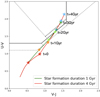 |
Fig. A.1. Galaxies with different star formation duration times in SFHs (see Fig. 4). The green line is a duration of 1 Gyr, and the red line is a duration of 4 Gyr, both with a quenching timescale of 1 Gyr. The star symbols show the time after the start of quenching. Symbols of the same colour on different curves show the same time after quenching. |
Then we discuss the evolution of spectral features along the model paths. We use the high-resolution mode of CIGALE to output high-resolution SED of model galaxies at each position and calculate the equivalent widths (EWs) of Hδ and [OII] line features. Figure A.2 shows the fast and slow quenching paths with blue and red curves, respectively. The EWs of Hδ (black) and [OII] (light blue) at each point are presented next to the position. A negative EW represents the absorption feature, while a positive EW represents the emission feature. All EWs are calculated using the same method as in Sect. 5.1. We can see that the Hδ absorption line strength first increases and then decreases along the evolution paths. In the RQG region, both the fast-quenching and slow-quenching galaxies show strong Hδ absorption. For the fast-quenching galaxy there is no [OII] emission left. However, the Hδ absorption is weaker for the slow-quenching galaxy compared to the fast-quenching galaxy due to its longer quenching timescale, and the [OII] emission is stronger due to remaining star formation. These features are also consistent with the spectral confirmation in Sect. 5.1. In conclusion, our boundary selection is reasonable and consistent with the spectral features of RQGs.
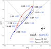 |
Fig. A.2. Equivalent width of the Hδ absorption line and [OII] emission line at different positions in UVJ space. The two evolutionary tracks are of galaxies with 1 Gyr star formation duration but different quenching timescales, E(B-V)=0.15. Values in blue show the EW of [OII] emission lines, values in black the EW of Hδ absorption lines. A negative value represents absorption, and a positive value represents emission. |
Finally, we discuss how dust attenuation affects the evolution paths. We use different dust parameters in CIGALE and calculate the evolution paths on the UVJ diagram. In Fig. A.3, we show the evolution path with E(B-V)=0.15 and 0.2. The paths are shifted to the top right, and the reddening vector of E(B-V)=0.1 is also plotted in the diagram. We note that for both E(B-V) values, the fast quenching and slow quenching tracks are still in the fast (purple) and slow (orange) quenching regions. Considering that RQGs should have a certain amount of dust as the fuel of the remaining star formation, the dust attenuation will lead to some contamination, but will not affect the separation of fast and slow quenching much.
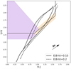 |
Fig. A.3. Effect of dust attenuation. Solid tracks are paths with E(B-V)=0.15 dust attenuation. Dashed tracks are E(B-V)=0.2 dust attenuation. The arrow on the plot shows the reddening vector of E(B-V)=0.1. |
Appendix B: Binning information for result
In this appendix we introduce the bin information of all bins we used in Sect. 4. The first column of all the tables shows the ranges of bins, and the second column shows the number of galaxies in these bins.
Information of mass bins in all environments (left panel in Figs. 5, 7, and 12).
Information of local density bins with all mass (left panels in Figs. 6 and 8, and right panels of Fig. 12).
Top table: Information of mass bins in low local density (middle panel in Figs. 5 and 7). Bottom table: Information of mass bins in high local density (right panel in Figs. 5 and 7).
Top table: Information of mass bins in low local density (middle panel in Figs. 6 and 8). Bottom table: Information of mass bins in high local density (right panel in Figs. 6 and 8).
Top table: Mass bin information in Fig. 9. Middle table: Local density bin information in Fig. 10. Bottom table: Redshift bin information in Fig. 11.
Appendix C: Detailed information of spectral confirmation
In this appendix we list the information of galaxy spectra in Sect. 5.1 and Fig. 14 in Table C.1. All IDs are the IDs of galaxies in Laigle et al. (2016).
Information of galaxy spectra in Sect. 5.1 and Fig. 14. The first column gives the source of the spectroscopic data. The second column shows galaxy ID. The third and fourth columns show rest-frame UVJ colours. The fifth and sixth columns show equivalent width of Hδ and [OII] lines; a positive value means emission and a negative value means absorption. The seventh column shows the type of galaxy classified by rest-frame UVJ colours.
All Tables
Information of mass bins in all environments (left panel in Figs. 5, 7, and 12).
Information of local density bins with all mass (left panels in Figs. 6 and 8, and right panels of Fig. 12).
Top table: Information of mass bins in low local density (middle panel in Figs. 5 and 7). Bottom table: Information of mass bins in high local density (right panel in Figs. 5 and 7).
Top table: Information of mass bins in low local density (middle panel in Figs. 6 and 8). Bottom table: Information of mass bins in high local density (right panel in Figs. 6 and 8).
Top table: Mass bin information in Fig. 9. Middle table: Local density bin information in Fig. 10. Bottom table: Redshift bin information in Fig. 11.
Information of galaxy spectra in Sect. 5.1 and Fig. 14. The first column gives the source of the spectroscopic data. The second column shows galaxy ID. The third and fourth columns show rest-frame UVJ colours. The fifth and sixth columns show equivalent width of Hδ and [OII] lines; a positive value means emission and a negative value means absorption. The seventh column shows the type of galaxy classified by rest-frame UVJ colours.
All Figures
|
Fig. 1. Aperture density map of a redshift slice at z ∼ 0.5 − 0.6. The colours show aperture density in the logarithm scale. The red contours indicate the edge of 3σ peaks, and the blue contours the edge of 1σ regions. The area outside the 1σ contours is identified as field. This kind of density map is plotted for all redshift slices to select cluster candidates and construct the field sample, which is used to make a statistical subtraction of the field average density. Stars indicate the confirmed cluster candidates analysed in this work. |
| In the text | |
|
Fig. 2. Redshift distribution of three typical cases. The histograms show the distribution of photometric redshifts of galaxy members. Top panel: cluster candidate located within one redshift slice; the vertical line in this panel gives the mean photometric redshift value. Middle panel: flat distribution, indicating that this overdensity is not a physically connected structure. Bottom panel: distribution of a real structure, but its peak is close to the edge of our selection redshift slice, missing a large fraction of its galaxy members. |
| In the text | |
|
Fig. 3. Rest-frame UVJ diagram used to classify galaxy populations. The solid black lines are boundaries in Schreiber et al. (2018). The dashed lines are the modified boundaries used in this work (see Sect. 3.1.2). The red dots are QGs; blue dots are SFGs; purple and orange dots are both RQGs. The colour-shaded regions are RQG regions, and they are divided into fast- and slow-quenching regions. The two regions are divided by black and red diagonal solid lines according to evolution tracks (red and purple lines) of two model galaxies with a 1 and 0.1 Gyr quenching timescale, respectively (see Sect. 3.2). The arrow is the dust extinction vector corresponding to E(B − V)=0.1. Numbers indicate the different regions: 1 and 2 are fast-quenching RQG; 3 and 4 are slow-quenching RQG; 5 and 6 are QG; 7 is SFG. |
| In the text | |
|
Fig. 4. Star formation history models with a constant star formation period followed by exponentially declining quenching period with τ = 0.1 and 1 Gyr. |
| In the text | |
|
Fig. 5. Mass dependence of Q.E. Left panel: dependence in all environments in our sample cluster candidates. Middle and right panels: dependence in two subsamples divided by local density. The total number of galaxies in the two subsamples are the same. The number to the left of each data point is the number of RQGs in this mass bin, while the number to the right is the number of SFGs. The total number of SFGs or RQGs in the middle and the right panels is the same as the number of the cluster candidates in the left panel. Errors are propagated based on the Poisson statistics error of each population in each bin. |
| In the text | |
|
Fig. 6. Environmental dependence of Q.E. Left panel: dependence of all masses. Middle and right panels: dependence in two subsamples divided by stellar mass. The total number of galaxies in the two subsamples are the same. The number to the left of each data point is number of RQGs in this mass bin, while the number to the right is the number of SFGs. The total number of SFGs or RQGs in the middle and the right panels is the same as the number of the cluster candidates in the left panel. Errors are propagated based on the Poisson statistics for each population in each bin. |
| In the text | |
|
Fig. 7. Mass dependence of Q.S. Left panel: dependence in all environments in our sample of cluster candidates. Middle and right panels: dependence in two subsamples divided by local density (same bin division as in Fig. 5). The number to the left of each data point is the number of RQGs in this mass bin, while the number to the right is the number of QGs. The total number of QGs or RQGs in the middle and right panels is the same as the number of cluster candidates in the left panel. Errors are propagated based on the Poisson statistics for each population in each bin. |
| In the text | |
|
Fig. 8. Environmental dependence of Q.S. Left panel: dependence for all environments. Middle and right panels: dependence in different mass bins (same bin division as in Fig. 6). The number to the left of each data point is the number of RQGs in this density bin, while the number to the right is the number of QGs. The total number of QGs or RQGs in the middle and the right panels is the same as the number of cluster candidates in the left panel. Errors are propagated based on the Poisson statistics for each population in each bin. |
| In the text | |
|
Fig. 9. Quenching timescale increase with stellar mass. The number to the left and right of each data point respectively show the number of slow- and fast-quenching galaxies for each mass bin. Errors are derived based on the Poisson statistics for each population in each bin. |
| In the text | |
|
Fig. 10. Quenching timescale does not have a clear relation with local density. The number to the left and right of each data point respectively represent the number of slow- and fast-quenching galaxies for each mass bin. Errors are derived based on the Poisson statistics error of each population in each bin. |
| In the text | |
|
Fig. 11. Quenching timescale decrease with redshift. The number to the left and right of each data point respectively represent the number of slow- and fast-quenching galaxies for each mass bin. Errors are derived based on the Poisson statistics error of each population in each bin. |
| In the text | |
|
Fig. 12. In this figure, we show results of Q.E. and Q.S. in fast- and slow-quenching galaxies separately. Slow-quenching galaxies (same as long visibility timescale galaxies) are marked with orange points, while fast-quenching galaxies (same as short visibility timescale galaxies) are marked with light blue points. |
| In the text | |
|
Fig. 13. Comoving number density evolution of all RQGs, slow-quenching RQGs, and fast-quenching RQGs. To increase the statistics, all galaxies are put into two bins, 0.5 < z < 0.75 (low redshift) and 0.75 < z < 1.0 (high redshift), consisting of 1468 and 2419 RQGs, respectively. |
| In the text | |
|
Fig. 14. UVJ-selected RQGs with strong absorption lines (in blue) and without strong absorption lines (in red) and their rest-frame UVJ colour uncertainties. Star symbols are galaxies without strong [OII] emission, while squares are galaxies with strong [OII] emission lines. Crosses are galaxies that are not selected as RQG in the UVJ diagram, but with RQG spectral features and their UVJ colour uncertainties. The arrow shows the reddening vector. |
| In the text | |
|
Fig. 15. Two checked galaxy spectra (in observed frame). Spectral features are indicated with green dashed lines. An artificial break between two chips of the DEIMOS spectrograph is shown as a grey shaded area. Top panel: typical spectrum for strong Balmer absorption line galaxy, at z = 0.864. Bottom panel: typical spectrum for weak Balmer absorption line galaxy, at z = 0.553. |
| In the text | |
|
Fig. 16. Comparison between comoving number density of this work (RQG in traditional UVJ selection region) and Wilkinson et al. (2021) (PSB) in the COSMOS field. The five redshift bins in this plot are 0.5−0.6, 0.6−0.7, 0.7−0.8, 0.8−0.9, and 0.9−1.0. |
| In the text | |
|
Fig. A.1. Galaxies with different star formation duration times in SFHs (see Fig. 4). The green line is a duration of 1 Gyr, and the red line is a duration of 4 Gyr, both with a quenching timescale of 1 Gyr. The star symbols show the time after the start of quenching. Symbols of the same colour on different curves show the same time after quenching. |
| In the text | |
|
Fig. A.2. Equivalent width of the Hδ absorption line and [OII] emission line at different positions in UVJ space. The two evolutionary tracks are of galaxies with 1 Gyr star formation duration but different quenching timescales, E(B-V)=0.15. Values in blue show the EW of [OII] emission lines, values in black the EW of Hδ absorption lines. A negative value represents absorption, and a positive value represents emission. |
| In the text | |
|
Fig. A.3. Effect of dust attenuation. Solid tracks are paths with E(B-V)=0.15 dust attenuation. Dashed tracks are E(B-V)=0.2 dust attenuation. The arrow on the plot shows the reddening vector of E(B-V)=0.1. |
| In the text | |
Current usage metrics show cumulative count of Article Views (full-text article views including HTML views, PDF and ePub downloads, according to the available data) and Abstracts Views on Vision4Press platform.
Data correspond to usage on the plateform after 2015. The current usage metrics is available 48-96 hours after online publication and is updated daily on week days.
Initial download of the metrics may take a while.