| Issue |
A&A
Volume 666, October 2022
|
|
|---|---|---|
| Article Number | A189 | |
| Number of page(s) | 33 | |
| Section | Stellar atmospheres | |
| DOI | https://doi.org/10.1051/0004-6361/202243281 | |
| Published online | 28 October 2022 | |
Stellar wind properties of the nearly complete sample of O stars in the low metallicity young star cluster NGC 346 in the SMC galaxy★
1
Institut für Physik und Astronomie, Universität Potsdam,
Karl-Liebknecht-Str. 24/25,
14476
Potsdam, Germany
e-mail: This email address is being protected from spambots. You need JavaScript enabled to view it.
2
Department of Physics and Astronomy, University College London,
Gower Street,
London
WC1E 6BT, UK
3
Zentrum für Astronomie der Universität Heidelberg, Astronomisches Rechen-Institut,
Mönchhofstr. 12–14,
69120
Heidelberg, Germany
4
Armagh Observatory and Planetarium,
College Hill, Armagh,
BT61 9DG
Northern Ireland, UK
5
Institute of Astrophysics,
KU Leuven, Celestijnlaan 200D,
3001
Leuven, Belgium
6
Institute of Astronomy and Astrophysics,
Academia Sinica, No. 1, Sec. 4, Roosevelt Rd., Taipei,
10617
Taiwan, R.O.C.
7
Dept. Astronomy, University of Wisconsin,
Madison, WI, USA
Received:
7
February
2022
Accepted:
6
July
2022
Abstract
Context. Massive stars are among the main cosmic engines driving the evolution of star-forming galaxies. Their powerful ionising radiation and stellar winds inject a large amount of energy in the interstellar medium. Furthermore, mass-loss (Ṁ) through radiatively driven winds plays a key role in the evolution of massive stars. Even so, the wind mass-loss prescriptions used in stellar evolution models, population synthesis, and stellar feedback models often disagree with mass-loss rates empirically measured from the UV spectra of low metallicity massive stars.
Aims. The most massive young star cluster in the low metallicity Small Magellanic Cloud galaxy is NGC 346. This cluster contains more than half of all O stars discovered in this galaxy so far. A similar age, metallicity (Z), and extinction, the O stars in the NGC 346 cluster are uniquely suited for a comparative study of stellar winds in O stars of different subtypes. We aim to use a sample of O stars within NGC 346 to study stellar winds at low metallicity.
Methods. We mapped the central 1′ of NGC 346 with the long-slit UV observations performed by the Space Telescope Imaging Spectrograph (STIS) on board of the Hubble Space Telescope and complemented these new datasets with archival observations. Multi-epoch observations allowed for the detection of wind variability. The UV dataset was supplemented by optical spectroscopy and photometry. The resulting spectra were analysed using a non-local thermal equilibrium model atmosphere code (PoWR) to determine wind parameters and ionising fluxes.
Results. The effective mapping technique allowed us to obtain a mosaic of almost the full extent of the cluster and resolve stars in its core. Among hundreds of extracted stellar spectra, 21 belong to O stars. Nine of them are classified as O stars for the first time. We analyse, in detail, the UV spectra of 19 O stars (with a further two needing to be analysed in a later paper due to the complexity of the wind lines as a result of multiplicity). This more than triples the number of O stars in the core of NGC 346 with constrained wind properties. We show that the most commonly used theoretical mass-loss recipes for O stars over-predict mass-loss rates. We find that the empirical scaling between mass-loss rates (Ṁ) and luminosity (L), Ṁ ∝ L2.4, is steeper than theoretically expected by the most commonly used recipes. In agreement with the most recent theoretical predictions, we find within Ṁ ∝ Zα that α is dependent upon L. Only the most luminous stars dominate the ionisation feedback, while the weak stellar winds of O stars in NGC 346 and the lack of previous supernova explosions in this cluster restrict the kinetic energy input.
Key words: stars: winds, outflows / stars: individual: NGC 346 SSN18 / Magellanic Clouds / stars: evolution
Based on observations with the NASA/ESA Hubble Space Telescope, which is operated by the Association of Universities for Research in Astronomy, Inc., under NASA contract NAS 5-2655. Also based on observations collected at the European Organisation for Astronomical Research in the Southern Hemisphere.
© M. J. Rickard et al. 2022
 Open Access article, published by EDP Sciences, under the terms of the Creative Commons Attribution License (https://creativecommons.org/licenses/by/4.0), which permits unrestricted use, distribution, and reproduction in any medium, provided the original work is properly cited.
This article is published in open access under the Subscribe-to-Open model. This email address is being protected from spambots. You need JavaScript enabled to view it. to support open access publication.
1 Introduction
Massive stars (Minitial ≳ 8 M⊙) are a critical component in the understanding of galaxy evolution. Their feedback sets the conditions for star formation and determines the fates of star clusters. Massive stars, their winds, and their evolution are still poorly understood, especially at low metallicity (Z).
The Small Magellanic Cloud (SMC) is a nearby dwarf galaxy at d = 61 kpc (distance modulus, DM = 18.9 dex, Hilditch et al. 2005). It has a metallicity 5–7 times lower than the Galaxy (Dufour et al. 1982; Larsen et al. 2000; Trundle et al. 2007). Thus the SMC offers an excellent laboratory to study massive stars in environments that resemble the earlier cosmic epochs. The brightest and largest H ii region in the SMC is LHA 115-N 66 (Henize 1956). Supernovae have not occurred yet in N 66 (Danforth et al. 2003), making it the closest unpolluted laboratory optimally suited for studies of massive stars at low Z. N 66 is ionised by the young compact cluster NGC 346 (Fig. 1), which contains about half of all O-type stars in the entire SMC (Massey et al. 1989). NGC 346 is less than ~3 Myr old and is among the youngest and the most massive low-Z star clusters in the Local Group.
Walborn & Blades (1986) identified the major ionising source of the N 66 region as the O2 type star NGC 346 W 3 (SSN 9, Sabbi et al. 2007). Massey et al. (1989) used the CCD UBV photometry and spectroscopy to investigate the stellar content of NGC 346 and found 33 O type stars, with 11 being of type O6.5 or earlier; their catalogued stars have the prefix MPG (e.g. the O2 star NGC 346 W 3 is the same object as MPG 355). The field size in the Massey et al. (1989) survey was 2.5′ × 4.1′, that is, tracing nearly full extent of the N 66 H ii region (see upper panel in Fig. 1) but the core of NGC 346 remained unresolved prior to the study we present in this paper. Gouliermis et al. (2008) presented evidence that massive star feedback induces on-going star formation in N 66. The star formation rate in N 66 complex is ≈4 × 10⁻³ M⊙ yr−1 (Hony et al. 2015). Cignoni et al. (2011) found the star formation started in NGC 346 about 6 Myr ago, continued at a high rate (≥2 × 10⁻⁵ M⊙ yr−1 pc−2) for about 3 Myr, and is now progressing at a lower rate. They also noticed the deficiency of upper main sequence stars in NGC 346 and suggested that the youngest most massive stars did not yet have time to form.
Kudritzki et al. (1989) obtained optical spectra of four of the brightest stars in NGC 346, derived their high masses from spectroscopic analysis, and concluded that these four stars are responsible for half of the ionising flux in N 66. Walborn et al. (2000) present a UV and optical spectral atlas of 15 O stars in the SMC, among which 5 are in NGC 346. The UV spectra were measured by the Space Telescope Imaging Spectrograph (STIS) in high-resolution E140M echelle mode covering the wavelength interval 1150–1700 Å. These data were exploited by Bouret et al. (2003) who produced detailed spectroscopic analysis of six O stars in NGC 346. Sabbi et al. (2007) presented a catalogue of objects detected in the deep F555W (~V) and F814W (~I) Hubble Space Telescope (HST) ACS images of N 66 including NGC 346; their catalogue has prefix SSN, for example, the O2 star NGC 346 W 3 has aliases MPG 355 and SSN 9.
Up to now, the largest spectroscopic survey of NGC 346 massive stars was presented by Dufton et al. (2019). Using the VLT-FLAMES spectroscopy in the optical they determined spectral types of 47 O-type stars in the wide area around NGC 346, and estimated their temperatures, gravities, and projected rotational velocities using tlusty model atmospheres (Hubeny & Lanz 1995). However, optical spectra do not allow reliable measurements of stellar winds at lower mass-loss rates where there is no Hα emission.
The stellar winds of massive stars are best studied with UV spectroscopy. P-Cygni resonance lines formed in stellar winds as well as numerous metal lines are in the UV range, making UV spectroscopy the best tool to measure mass-loss rates, wind velocities, and to probe wind structure. Spectral analysis is completed by comparison of observed spectra to non-LTE models. These solve the radiative transfer equation in the co-moving frame whilst ensuring statistical equilibrium for rate equations (Hillier 1987; Hamann & Schmutz 1987; Harries et al. 2003; Sander et al. 2015).
The assumed mass-loss rates of massive stars are one of the key parameters defining their evolution. The most commonly employed mass-loss recipe for massive stars is the one of Vink et al. (2000, 2001), from here on  . These mass-loss prescriptions are implemented in stellar evolution models, population synthesis, and stellar feedback models and highly impact our understanding of the universe. However, increasing observational evidence question this theoretical prediction for low Z stars and indicate that the non-supergiant O stars have in fact much smaller mass-loss rates (Bouret et al. 2003, 2013; Hainich et al. 2018; Ramachandran et al. 2019). This highlights the need for larger samples of reliably derived low-Z massive stars wind parameters.
Mass-loss rate prescriptions as well as non-LTE stellar atmosphere models assume that stellar winds are homogeneous and spherically-symmetric on sufficiently large scales. However, the time series observations of Galactic massive stars consistently show the presence of discrete absorption components (DACs) moving towards the bluest extent of the absorption trough in UV wind profiles over the stellar rotation time-scale (Kaper et al. 1996; Massa & Prinja 2015). Typically, DACs migrate towards the blueward end of the absorption trough, while stationary narrow absorption components (NACs) are constant within the velocity space. The DACs are interpreted as a spectroscopic evidence for the large-scale structures in the winds of rotating stars, known as co-rotating interaction regions (CIRs, Mullan 1984; Cranmer & Owocki 1996; Lobel & Blomme 2008). While well established in Galactic O stars, very little is known about line profile variability of their SMC counterparts. In this paper, we investigate this question whenever we have multi-epoch UV observations, and discuss how wind line profile variability affects the measurements of stellar wind properties.
With the above key goal, the present study uses long slit UV spectroscopic observations to dissect the heart of the N 66 star forming region and measure for the first time the UV spectra of the nearly complete census of O stars in the dense parts of NGC 346 cluster (see lower panel in Fig. 1). In this work, we more than triple the number of the NGC 346 O stars spectroscopically analysed in the UV, and hence we draw robust conclusions on the wind properties of young O stars in general.
In Sect. 2, we describe our new HST STIS UV observations, our search for complementary archival HST observations, and introduce supplementary Multi Unit Spectroscopic Explorer (MUSE) Integrated Field Unit (IFU) observations. In Sect. 3, we describe the spectroscopic analyses using the synthetic spectra from models generated with the Potsdam Wolf–Rayet (PoWR) code to constrain mass-loss rates and other wind parameters and compare these to theoretical predictions and previous observations. Where multi-epochs exist, we compare observations of the wind profiles to look for signs of variability and large-scale wind structure. In Sect. 4, we detail our results for each target and the relationships derived. The discussion is presented in Sect. 5, while the conclusions are drawn in Sect. 6.
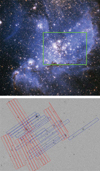 |
Fig. 1 NGC346 in the SMC. Top panel: optical colour composite of HST ACS image of the H ii region N 66, covering a total area of 3.5′ × 3.5v (≈62 pc × 62 pc at d = 61 kpc) on the sky. North is up, and east is to the left. The cluster of bright stars in the centre of the image is NGC 346. Credit: A. Nota (ESA/STScI). Lower panel: zoom to the region indicated by the green box in the top panel. The rectangles show our spectroscopic mosaic covering the central part of NGC 346. The GO 15112 STIS G140L slit positions are in red, while GO 8629 slit positions are in blue, see text for details. Background F225W image from HST archive (GO 12940). |
2 Observations
Our goal is to study stellar winds which are best observed in UV resonance lines. Therefore, the core of our observing samples are UV spectroscopy. These observations are complemented by optical spectra for each of our sample stars. Because the SSN catalogue overlaps completely with all MPG objects, throughout this paper we use the SSN numbers as star identifiers. A full list of the archival observations exploited for this work is contained within Appendix A.
2.1 Ultraviolet spectroscopy
HST observations were made using the STIS with the G140L grism in the long slit grating mode. All slits are 25″ × 2″ except for one where the luminosity of the brightest object required the use of a 25″ × 0.2″ slit. A total of 20 observations were made with General Observer programme 15112 (PI L. Oskinova). These are combined with twelve similar G140L observations from the HST archive (GO 8629, PI F. Bruhweiler). These observations mosaic the central 1′ of NGC 346.
Each of the 2D spectra are integrated across the wavelength range and for each 2D spectra a plot of Y pixel positions to flux is examined. A simple peak finding routine located all sources for spectral extraction. Background regions are identified from sections along the slit of ten pixels in length or greater with a continuous range of less than 0.5 σ deviation from the median flux value from the whole length of the slit. For each potential star to extract, two background regions, one above and one below the target, are selected. For the next step, the 1D spectra are extracted from the 2D spectra using the CALSTIS software package for HST data processing (Sohn et al. 2019). The extract_1d function extracts a 1D spectrum based on a pixel position for the centre of the object as well as the pixel offset and widths of the two background regions.
Of the 247 spectra successfully extracted from both observation sets, including multiple spectra for some sources with overlapping slits, 61 OB stars have signal-to-noise (S/R) >10. In this work, we consider only O stars; B type stars will be considered in future work. These spectra have a resolution of R ~ 2400–2950. The spectra for all O type stars extracted from the observations are shown in Fig. 2.
A search of the Mikulski Archive for Space Telescopes (MAST) was conducted for additional archival spectra. For four of the O star sources, SSN 9 (MPG 355), SSN 13 (MPG 324), SSN 15 (MPG 368), and SSN 18 (MPG 487), high resolution (R = 45 800) echelle spectra were identified from the HST GO 7437 (PI: D. J. Lennon). These were previously analysed by Bouret et al. (2003, 2013). The star SSN 17 was observed with HST GO 7667 (PI: R. Gilliland) in the G140M mode. These observations are a series of long slit high resolution (R ~ 11400–17400) spectra, with incrementally increasing central wavelengths. To assemble the full spectrum, each extracted 1D spectrum is spliced using the IRAF SPLICE function. In addition, a E140M spectrum of SSN 11 was obtained as part of GO 15837 (PI: L. Oskinova) and two E140M spectra of SSN 9 were obtained during GO 16098 (PI: J. Roman-Duval), as apart of the ULLYSES Director Discretionary Time (DDT) programme.
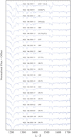 |
Fig. 2 Normalised UV spectra of all identified O stars extracted within the G140L observations of both GO 15112 and GO 8629. |
Stellar and wind parameters roadmap.
2.2 Far ultraviolet spectroscopy
Four of the brightest objects within our sample, SSN 7, SSN 9, SSN 11, and SSN 13, have been observed with the Far Ultraviolet Spectroscopic Explorer (FUSE). We accessed spectra from the FUSE Legacy in the Magellanic Clouds online archive (Blair et al. 2009), covering a range in the Far Ultraviolet (FUV) of 900–1190 Å. Lines within the FUV that are useful for wind diagnostics inculde the P V λ 1118, 1128 doublet, which is a useful diagnostic of wind structure such as macroscopic clumping (Oskinova et al. 2007).
2.3 Optical spectroscopy
NGC 346 has been a target of multiple optical spectroscopic surveys (e.g. Evans et al. 2006). We use the ESO VLT integral field spectrograph (MUSE) to observe the same central 1′ of NGC 346 as covered by the STIS mosaic (Programme ID 098.D-0211(A), PI WR Hamann). The results of MUSE observations will be detailed in a forthcoming publication (M. Rickard, in prep.). For this work, we combined three of our data cubes with the highest S/R and extracted from this the optical and near infrared spectra (R ~ 1770–3590, 4620–9265 Å) of all the O stars in our sample.
Furthermore, we carefully search ESO VLT archives and whenever available, use existing archival spectra. Specifically for some of our objects, spectra are available from the Fibre Large Array Multi Element Spectrograph (FLAMES) from the GIRAFFE spectrograph (R ~ 5000–2300, 3850–6690 Å depending on object, as detailed in Table A.1). This data was presented by Dufton et al. (2019). Therefore, for all our 19 analysed O stars, we have assembled UV and optical spectroscopy which allows for detailed multi-line spectroscopic analysis.
3 Data analysis
The roadmap describing the methods we use for determining the various stellar properties of each O star in our sample stars is detailed in Table 1. In this section, we provide additional information for each step.
3.1 Spectral typing
Commonly used spectral typing classification schemes are based on optical spectra, typically using lines blueward of 4600 Å (Conti & Alschuler 1971; Walborn & Fitzpatrick 1990; Sota et al. 2011). This is not possible for our MUSE spectra due to their wavelength range which covers λ4620–09350 Å. As all of our objects have MUSE spectra, we follow the methods described by Bodensteiner et al. (2020) and Kerton et al. (1999) to determine spectral type based on lines available within MUSE.
Bodensteiner et al. (2020) assign a spectral type for O types based on the equivalent widths (Wλ) of He i λ 5411 and He i λ 6678 In this work, we are interested in O type stars and the border between O9.5 V and B0V spectral type. According to Bodensteiner et al. (2020), the Wλ He ii λ 5412 will be below ~0.1 Å for spectral types later than B0.5. Therefore we exclude all such objects.
Kerton et al. (1999) developed a spectral type classification for heavily reddened O stars using the ratio of Wλ (He i λ4922/He ii λ 5411). We take advantage of this by ordering the MUSE spectra of our candidate O V to B0 V stars according to the ratio of Wλ He i λ4922 to Wλ He ii λ 5411(Fig. 3). We use the spectral types determined by Dufton et al. (2019) and others based on FLAMES spectra, combined with this spectral sequence to assign spectral types to stars in our sample. Finally, 21 stars within the STIS mosaic are identified as having O spectral type (Table 2).
All newly identified O type stars have strong He ii λ4686 absorption, and so are assigned the dwarf luminosity class. The ratio of Wλ He ii λ 4686/Wλ He i λ 4471 > 1.1 identifies O stars with a Vz luminosity class (Arias et al. 2016). Amongst the O type stars in our sample with archival FLAMES spectra which covers the He i λ4471 and He ii λ4542 lines, only SSN 31 has the ratio >1.1 and hence we assign it the Vz luminosity class.
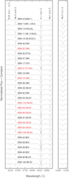 |
Fig. 3 Normalised MUSE spectra of all candidate OV-B0 V types stars in our sample. Black labels denote spectral types from literature. Red and bold labels denote spectral type assigned from this work. |
Spectral types of O stars in this work, with references where drawn from published literature.
3.2 Interstellar medium (ISM) line modelling and spectra wavelength correction for slit position
High resolution HST UV echelle E140M spectra show multiple lines too narrow to be of stellar origin and are instead attributed to the intervening ISM. These lines include Si ii λ 1260.4, O i λλ 1302.1, 1304.9 doublet, and C ii λλ 1334.5, 1335.7 doublet, as well as Si ii λ 1526.7 and C iv λλ 1548.2, 1550.8 doublet, which contaminate low resolution observations of the C iv λλ 1548.2, 1550.8 wind lines and the photospheric lines of the same ions.
For the G140L spectra, the position of the source across the 2″ width of the slit can shift the wavelength of the extracted spectra by ~ 10 Å, therefore the known positions of ISM lines can be used to improve the wavelength calibration of the extracted spectra (Fig. 4). The Si iiλ 1260.4, O i λλ 1302.1, 1304.9 doublet and C ii λλ 1334.5, 1335.7 doublet ISM lines are modelled following the formalism from Groenewegen & Lamers (1989) to simulate absorption based on a column density from the extinction, E(B−V), with a Lorentzian absorption profile assuming the natural line broadening dominates and using the square root part of the curve of growth. Two components of ISM absorption are simulated, from Galactic ISM and the SMC ISM. All our sources are within 1′ of each other and hence we use a uniform Galactic extinction for the Galactic line of sight, which we adopt as E(B−V) = 0.07 mag. As a result, the model Spectral Energy Distribution (SED, see Sect. 3.5) is modified by both a galactic extinction which is constant for all targets and an SMC contribution which is varied for each target.
To simplify the ISM model, we assume a standard gas to dust ratio for the SMC. To account for the low SMC metallicity we scale the SMC hydrogen column density from the Galactic hydrogen column density NH = 3.8 × 10²¹ × E(B−V) (Groenewegen & Lamers 1989) by a factor of 7. Column densities of the relevant components of the ISM are then calculated from relative solar abundances scaled in the same way. A value of 165 km s−1 is used for radial velocity (RV) shift of the SMC ISM lines as this is found to best match the relative wavelength difference between the galactic and SMC components. This value is similar to that of stars within the SMC (Bouret et al. 2003). A Voigt function is applied to describe the line shape. A cool ISM temperature of 10 K is selected for the Galactic ISM line contribution, while a temperature of 16 000 K is adopted for the SMC component to this line of sight, based on radio continuum studies (Reid et al. 2006). This leaves only the turbulent velocity as a free parameter to adjust to match the profile strength. The Galactic contribution is kept constant with a value of 10 km s−1. In the SMC ISM, turbulent velocity is adjusted for each star based on the shape of the observed Si ii, O i, and C ii ISM lines, with values within the range of 10–30 km s−1 (e.g. Fig. 4).
As a next step, a wavelength shift is applied to each G140L spectrum to match the positions of the observed ISM lines with those modelled in our synthetic spectrum. Due to the instrument resolution and instrumental broadening, the precision of our wavelength calibration method is of the order of ±0.1 Å.
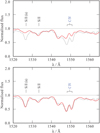 |
Fig. 4 C ivλλ 1548.2, 1550.8 wind profile in the UV spectrum of SSN 31 (O7.5 Vz). Synthetic spectrum in red, observations in black. Top panel: synthetic spectrum with wind parameters v∞ = 1000 km s−1, β = 0.8, D = 10, and |

3.3 Stellar atmosphere models
In this work, we use the state-of-the-art PoWR code, which is a non-LTE model atmosphere code for hot stars with expanding atmospheres that can be applied to a range of metallicities (Hainich et al. 2014, 2015; Oskinova et al. 2011; Shenar et al. 2015). PoWR iteratively solves the radiative transfer equations in the co-moving frame while balancing the rate equations for each ion level to ensure statistical equilibrium. The model produces a synthetic spectrum based on a detailed model that accounts for mass-loss, line blanketing, and wind clumping. Full details of PoWR are described within Gräfener et al. (2002); Hamann & Gräfener (2004); Sander et al. (2015); Hainich et al. (2015). Detailed atomic data for a range of ion levels is used along with a ‘superlevel’ approach to account for ‘iron blanketing’ (Gräfener et al. 2002). PoWR includes the handling of microclumping, dense regions within the wind smaller than the mean free photon path length.
In the subsonic part of the atmosphere, the velocity field is defined such that a hydrostatic density stratification is approached (Sander et al. 2015). In the supersonic part of the atmosphere, the velocity field is defined by a so-called β-law (Castor et al. 1975), given by;
 (1)
(1)
where r0 ~ R*.
PoWR relates temperature to radius and luminosity via the Stefan-Boltzmann law ( ). T* is defined within the PoWR code as the temperature at the Rosseland continuum optical depth. The effective temperature is typically defined at τeff = 2/3. However, as the winds of O stars are optically thin, the difference between T* and Teff is negligible. Group elements are incorporated in PoWR models with the atomic data for H, He, C, N, O, Si, Mg, S, and P, with Fe group elements included with a ‘superlevel’ approach (Gräfener et al. 2002).
Clumping within the PoWR code is specified in the form of a density contrast D, which denotes the inverse of the filling factor
 (2)
(2)
where the medium between the clumps is assumed to be void. As microclumping increases the density, this affects the wind recombination lines. Far ultraviolet lines are also sensitive to microclumping. However, in all the stars considered in the present paper with FUSE observations, the lines such as P V have no identifiable wind profile.
3.4 Temperature, surface gravity, and abundances
The temperature (T*) and surface gravity (log g) are determined by fitting the optical (MUSE) spectra to a published grid of PoWR models of SMC O stars (Hainich et al. 2019). These grids use the SMC abundances from Hunter et al. (2007) and Trundle et al. (2007), with additional elements scaled from solar abundances1 by 1/7 for ZSMC/Z⊙. Table 3 shows the abundances employed in the PoWR models grids. These grids have a resolution of 1000 K in T* and 0.2 dex in log g. The results of this process are included in Sect. C. The grids are publicly available and can be downloaded from the PoWR website2. Full details of the MUSE observations and data analysis will be presented in a forthcoming paper (Rickard et al., in prep.).
In the majority of the optical spectra, there are few metal lines available to individually tailor abundances. Therefore, the grid abundances as detailed in Table 3, are carried forward into the individual models for each O star. The exception to this is the CNO abundances for the hottest stars in our sample. In these cases, CNO abundances are adjusted per star based upon UV and optical metal lines, as detailed in Sect. 4.1.
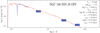 |
Fig. 5 Example SED illustrating the method to estimate L and E(B−V). Spectrum and photometry (HST F225 W, F555W, and F814W) of SSN 36 are shown by blue line and boxes correspondingly. The best model, modified for extinction (Sect. 3.5), is in red. Model parameters are listed in the insert. |
Abundances and Ions used within the PoWR model SMC grid.
3.5 Luminosity
The bolometric luminosity of each star is determined using its flux calibrated UV spectrum. This is compared to a synthetic SED modified for extinction (Sect. 3.2). The synthetic spectra are modified using the Seaton (1979) law for the Galactic components and the Bouchet et al. (1985) extinction law while for the SMC component using the PoWR code plotting package which has a form of these laws integrated across the whole SED. The combined Galactic and SMC value of E(B−V) is selected to match both the slope of the extinction modified synthetic SED to the observations and the width of the Lyα absorption compared to a synthetic Lyα profile generated following the formalisation in Groenewegen & Lamers (1989), see example Fig. 5. With a model luminosity and extinction, the PoWR code generates a model flux continuum which is then used to normalise the observed spectra.
The synthetic SED is shifted to match the observed UV spectra and photometry from HST bands F555W and F814W (Sabbi et al. 2007), and F225W DAOPhot extraction from the Hubble Legacy Archives3. log L can be found to ±0.01 dex and E(B−V) to ±0.01 mag, but the degeneracy between the two means that an error of ± 0.01 mag in E(B−V) translates to a total error of ±0.05 dex in log L.
3.6 Projected rotational velocities
For half of our sample stars the projected rotational velocities, v sin i, are taken from Dufton et al. (2019), calculated from TLUSTY fits to the FLAMES spectra. For the remaining objects, the photospheric He ii λ 4921 and λ 6678 lines within our MUSE spectra are examined with the iacob-broad tool (Simón-Díaz & Herrero 2014). This uses a combination of a Fourier Transform (FT) and a goodness of fit method to measure v sin i. The synthetic model spectra are then convolved with a Gaussian with a full width half maximum equal to the measured v sin i.
3.7 Terminal wind velocities
Terminal velocities (v∞) are measured from the blue edge of the black trough of a saturated wind profile. Only one O star in our sample has a wind profile that is fully saturated, aving a saturated N v λλ 1238.8, 1242.8 doublet. In an unsaturated wind profile, v∞ may be beyond the measurable blueward shift in velocity space of the profile. In this case, the blue edge of the absorption trough gives a lower limit to v∞. For stars where no wind profiles are seen in the UV spectra, we adopt a terminal velocity calculated from the escape velocity of the star following Lamers et al. (1995), scaled to SMC metallicity (Leitherer et al. 1992).
3.8 Microturbulence
In stellar atmosphere models, the microturbulent velocity parameter ξ(r) accounts for small scale turbulent motions. Within PoWR, this parameter is handled separately for the hydrostatic part of the atmosphere and for the expanding wind. For the hydrostatic part, a turbulent pressure term is incorporated in the hydrostatic equation, adding to the gas pressure term, in line with the arguments by Hubeny et al. (1991). By varying this value, we see that the value of ξ for the hydrostatic part of the wind has little impact on the synthetic spectrum and so adopt a constant ξ = 10 km s−1.
For the emergent spectrum of the stellar wind, we specify ξ(r) = max(ξmin, 0.1 · v(r)) (Shenar et al. 2015; Sander et al. 2015), where ξmin is dependent upon spectral type. A value of 10 km s−1 is commonly invoked for O stars, but earlier spectral types can be best matched by models with values as high as 25 km s−1. For the lines that are affected, a general trend of higher turbulent velocities for earlier spectral types and higher luminosity classes is determined (Bouret et al. 2003). We follow these results and set ξmin as detailed in Table 4.
Minimum turbulent velocities (ξmin [km s−1]) adopted according to spectral type (Bouret et al. 2003).
3.9 Wind parameters
For each O star within our sample, a tailored model is run with the fundamental stellar parameters of T*, log g, L, and abundances so far established. The velocity law exponent (β; Eq. (1)), mass-loss rate (![Mathematical equation: $\dot M\left[ {{M_ \odot }{\rm{y}}{{\rm{r}}^{ - 1}}} \right]$](/articles/aa/full_html/2022/10/aa43281-22/aa43281-22-eq11.png) ), and clumping factor (D; Eqs. (2) and (3)) are constrained by the fitting the diagnostic resonance P Cygni wind lines of the N v λλ 1238.8, 1242.8 doublet, the O v λ 1371.0 line, and the C iv λλ 1548.2, 1550.8 doublet. The mass-loss rate is measured by the overall strength of the wind profile. The selected β-law affects the shape of the blue-ward absorption.
), and clumping factor (D; Eqs. (2) and (3)) are constrained by the fitting the diagnostic resonance P Cygni wind lines of the N v λλ 1238.8, 1242.8 doublet, the O v λ 1371.0 line, and the C iv λλ 1548.2, 1550.8 doublet. The mass-loss rate is measured by the overall strength of the wind profile. The selected β-law affects the shape of the blue-ward absorption.
For our tailored models, we adopt clumping distribution using the equation:
 (3)
(3)
with clumping starting at vcl = 30 km s−1 (Hillier & Miller 1998). Models with a higher D have lower population of N v within the clumps due to recombination and so the N v λλ 1238.8, 1242.8 wind profile becomes less pronounced. The effect is smaller for the O v λ 1371.0 and C iv λλ 1548.2, 1550.8 wind profiles, and so the simultaneous adjustment of  and D is required whilst considering all three UV wind lines. The clumping factor, D, is limited to possible values of 1 (for a smooth wind), 5, 10, 20, 50, or 100 to limit the parameter space.
Eight stars in our sample (Table 5) have detectable wind profile in either the N v λλ 1238.8, 1242.8 or C iv λλ 1548.2, 1550.8 resonance lines. For these stars, the wind parameters are fitted simultaneously. Four among them have only slight blueward absorption in the C iv λλ 1548.2, 1550.8 profile. For the low resolution spectra, the ISM C iv λλ 1548.2, 1550.8 has the effect of enhancing the core of this wind line, see Fig. 10. The line contamination by the ISM means that very slight blue-ward asymmetry (≲300 km s−1) in the C iv λλ 1548.2, 1550.8 wind line cannot be determined from the G140L spectra.
The N v λλ 1238.8, 1242.8 line is sensitive to X-ray radiation field in stellar wind. However, the X-ray fluxes of individual stars in our sample are not unknown (Nazé et al. 2002). The single stars in the SMC seem to be intrinsically faint in X-rays, as shown in sensitive X-ray observations did not detect the O3V-type star SK 183 in the SMC (Oskinova et al. 2013). Since X-ray fluxes of our sample stars are not know, to avoid introduction of additional free parameters describing X-ray properties, we exclude X-rays from our models.
For stars without observed UV wind profiles, only an upper limit for  can be determined. In this case, β and D are the standard values for O stars (0.8 and 10 respectively, Hainich et al. 2019 and references therein).
3.10 Spectroscopic binaries
Dufton et al. (2019) have identified spectroscopic binaries in NGC 346 by subtracting two FLAMES spectra of different epochs from each other. This method can identify spectral binaries with RV variation ≳ 10 km s−1 between two observations. They also identify a number of SB2 and SB3 binaries within NGC 346. Our multi-epoch MUSE observations allow further identification of spectroscopic binaries via RV variations between epochs (Rickard et al., in prep.) with MSB used as a label (MUSE Spectroscopic Binary candidate) for this case, see Table 5. These results are preliminary, but have a good correlation with the spectroscopic binaries from Dufton et al. (2019) which is encouraging.
In the absence of spectral lines that can be attributed to a secondary, we consider a single star fit to be appropriate, as the secondary is going to be a considerably lower luminosity star with little contribution to the flux. On the other hand, when spectral lines are clearly seen from a second or even third component, such as in the SSN 7 and SSN 11 spectra, we do not fit a single star model. These objects will be considered in a forthcoming publication.
4 Results
In this section, we detail the results for each O star within our sample and present the general trends and relationships which emerge from our analysis. The full model, observed SED, and UV spectra for each object are included in Appendix D.
4.1 Individual stars
We present the model parameters of the synthetic spectra that match spectroscopic observations. For four stars (SSN 14, SSN 17, SSN 22, and SSN 31) we present the first measured wind parameters from UV observations. We also establish for the first time upper limits for wind parameters for eleven objects.
4.1.1 SSN 7 (MPG 435)
Massey et al. (1989) assigned the spectral type of O5.5If, assuming that the object is a single star. However, RV variations indicate that the star is a binary with a period of 24.2d (Niemela et al. 1986; Niemela & Gamen 2004). Dufton et al. (2019) confirm it as an SB1 binary. We also observe rapidly shifting lines within our MUSE observations (Rickard et al., in prep.). As described by Dufton et al. (2019), the N iv λ4058 emission line matches the RV of the primary therefore requiring the primary spectral subtype earlier than O5, with He i λ 4471 absorption and weak He ii λ 4686 emission indicating a spectral subtype O4 If. The secondary has a spectral type of O5-6 from He i λ4471 absorption being weaker than the He ii λ4542 absorption. With spectral lines and components attributable to the RV of the individual components, we identify SSN 7 as a potential object for which a spectral fit can be made with a binary composite model. Such a fit will be shown in a future paper.
Model Parameters derived for O stars within sample with a UV spectrum.
4.1.2 SSN 9 (MPG 355)
SSN 9 has the spectral type of O2 III(f*) from analysis by Walborn et al. (2000) and projected rotational velocity v sin i = 130km s−1 from Dufton et al. (2019). The E140M UV spectrum we use has previously been analysed by Bouret et al. (2003, 2013) who determined T* = 51.7 kK and log g = 4.00. This temperature is beyond the grid range, so we adopt the stellar parameters from Bouret et al. (2013) and find that synthetic spectra produced to be a good match to the optical He i and He ii lines.
Bouret et al. (2013) adopt N/N⊙ = 1.9. We find that N iv λλ 7105, 7111, 7123 triplet emission, not available to Bouret et al. (2013), is lower in the MUSE observations and is best matched by N/N⊙ = 1.5.
With an abundance of O/O⊙ = 0.2 as found by Bouret et al. (2013), we find that the emission line O iv λ4654 is over-estimated. We instead implement an abundance of O/O⊙ = 0.09 to explain this line better. However, this then leaves the O iv λλ 1337 1343 1344 absorption too weak. This line is heavily affected by the microturbulence. Bouret et al. (2013) experimented with values of ξmin ≥ 25km s−1 but we are unable to fit their value with other lines. With the lower O abundance we adopt due to the observed O iv λλ 7105, 7111, 7123 triplet emission we find ξmin = 35km s−1 to match O iv λλ1337 1343 1344.
Despite the lower O abundance, we are not able to match the O V λ1371 wind line even with D = 100. Bouret et al. (2013) reproduce this line with their higher O abundance and the wind parameters  , D = 50, and v∞ = 2800 km s−1. We find even with log
  and D = 100 that, while we match the C iv λλ 1548.2, 1550.8 wind profile, we are still unable to match the O V λ1371 (Fig. 6). By invoking a high density contrast (D = 200) we find a match to all UV wind lines and Hα with
  . We were unable to match the slope of the blue wing of the N v λλ 1238.8, 1242.8 doublet in any model. We speculate that a model which includes x-rays might better describe the shape of this line.
While there is evidence of a shift in the He ii lines in the MUSE observations (Rickard et al., in prep.), it was not noted by Dufton et al. (2019) as a spectral binary and there are no spectral lines that could be attributed to a secondary. As a result, the wind lines are entirely attributed to the primary.
At the bluest extent of the C iv λλ 1548.2, 1550.8 wind profile, a NAC is present. Due to the high v∞ of this wind, the NAC is close to the Si ii λ 1533 line but is of a greater strength and centered redward. SSN 9 has been observed with E140M grating as a part of the ULLYSES programme, enabling high resolution multiple epoch spectral comparisons (Fig. 7). This NAC feature can be seen to be shifting blueward on the timescale of hours.
4.1.3 SSN 11 (MPG 342)
The He i λ 4471 and He ii λ 4542 lines in the FLAMES spectra of SSN 11 show at least two distinct spectral line features. Massey et al. (2012) mentioned a third component, confirmed by Dufton et al. (2019) who show three components in both the He ii λ4542 and He ii λ4685.8 lines within the AAT-UCLES spectra they present. With 11 MUSE observations over ~10 days, we see three components in He i and He ii lines shifting with large (≥250 km s−1) RV changes over time. This is evident in lines such as the He i λ 5875.6 and He i λ 7065.3 lines.
Due to SSN 11 being an SB3, the T, and log g fit to the SMC grid cannot be relied on. The fit temperature we find is not consistent with the N iii λλ 4634, 4641 doublet emission. We do not attempt a single star fit for SSN 11 as we cannot reasonably believe our T* and log g is representative of the primary. We will present a three body solution to SSN 11 in a future paper (Rickard, in prep.).
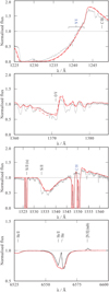 |
Fig. 6 Spectral observations of wind lines of SSN 9, normalised and compared to various models. The observed spectra of SSN 9 is shown by black line. Synthetic spectra with |


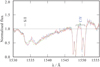 |
Fig. 7 Multi-epoch observations of SSN 9 C iv λλ 1548.2, 1550.8 UV wind profile. Green line: observation taken on 22-11-2000. Blue and red lines: observations taken on 01-09-2020 and separated by ~1 h, with the blue-line spectrum observed prior to the red-line spectrum. Each of these exposures is ~40 min. A feature can be seen moving blueward on the timescale of hours. |
4.1.4 SSN 13 (MPG 324)
This star has a spectral type of O4V((f)) from Walborn et al. (2000) and we use the rotational velocity v sin i = 113km s−1 from Dufton et al. (2019). We determine T* = 41 kK and log g = 3.8 from our MUSE observations. Bouret et al. (2003) find a higher temperature due to the balance of C iii λ 1176 to C iv λ1169. PoWR models also favour slightly higher temperatures when considering the carbon UV lines, so we adopt T* = 42 kK.
Bouret et al. (2003) show a model fit to the E140M spectra that we have used to aid our analysis. They require an N abundance of N/N⊙ = 0.2. We find agreement with PoWR, with this abundance being the best fit for both the N iii λλ1183, 1185 doublet, the N iv λ1718 absorption lines, and the N iii λλ4634, 4641 doublet emission and the N iii triplet λλ 7105, 7111, 7123 emission lines in MUSE, which were not available for the Bouret et al. (2003) analysis.
The wind parameters from Bouret et al. (2003) are  , β = 1.0, D = 10, and v∞ = 2300 km s−1. Our PoWR model fit to the observed wind profiles gives
  , β = 1.0, and v∞ = 2300 km s−1, with a higher clumping factor of D = 20. The small difference in mass-loss rate can be attributed to the difference of 0.2 dex in log g and 500 K in T* between our stellar parameters and those used by Bouret et al. (2003).
We assume that the deep absorption feature seen at the blue extent of the N v λλ 1238.8, 1242.8 absorption trough is a NAC. Thus when adjusting mass-loss rate, we select model that does not produce as deep a profile as would be required to match the depth of the NAC (Fig. 8).
4.1.5 SSN 14 (MPG 470)
This source is in a very crowded field (Fig. 9). We believe that SSN 14 is MPG 470 as both represent the brightest UV sources in their respective surveys within the tight group, as seen in Fig. 9, though Sabbi et al. (2007) do not make this connection. MPG 470 has previously been given a classification of O8.5III (Massey et al. 1989), but this classification is not supported by the wings of the observed MUSE He ii λ 4860 line which fit to a high log g = 4.4.
SSN 14 was observed twice in G140L long slit mode (Fig. 9). The SEDs from these observations have different slopes, though they both agree at the blue end of the UV. This would suggest that SSN 14 is the main contributor in UV. From the long slit sloping SE to NW, we extract two additional UV bright objects on the axis, such that these two objects are contaminants in the extraction of SSN 14 in the NE to SW long slit. We subtract these two flux calibrated spectra from the spectra of SSN 14. As these containments are shifted in the dispersion direction, they are shifted in to their observed frames based on the morphology of the ISM lines. The resultant observed SED of SSN 14 give the luminosity as L/L⊙ = 5.37 ± 0.05. We assign the spectral type of O8 V in this work. The fit to grid models yields T* = 33 kK and log g = 4.4.
This star is a known eclipsing binary with a period 9.7 days (Pawlak et al. 2016). However both the UV spectra taken in 2001 and in 2018 have nearly identical UV wind features. In the absence of a time series of spectra we model it as a single star. Both spectra show no wind profiles in any UV lines with the exception of C iv λλ 1548.2, 1550.8 which shows a very slight blueward asymmetry up to 600 km s−1 present in both spectra.
There is no emission in neither the N iii λλ4634, 4641 doublet, nor in the N iiiλλ7105, 7111, 7123 lines, suggesting that there is no surface N enrichment. For the UV spectra extracted from the long slits, contamination of other sources along the width of the slit means that the narrow UV metals lines are hard to attribute solely to SSN 14. A bright object also within the width of the slit will contribute to the spectrum observed but will be shifted in the wavelength direction. We attribute the broadening of the various N and C photospheric UV lines to this. As such, we do not use UV lines for abundance fitting and in the absence of any evidence for N enrichment in the MUSE spectra, we adopt the grid abundances.
The slight blueward asymmetry in the C iv λλ 1548.2, 1550.8 wind profile can be matched with the synthetic spectrum with  and v∞ = 600 km s−1. A density contrast D = 10 produces slight N v λλ 1238.8, 1242.8 blueward absorption, not present in the observations, so a slightly increased density of D = 20 is invoked (Fig. 10). This slight blueward asymmetry could be attributed to another object within the slit. However, due to the depth of the feature, it would require the contaminating object to be a significant contributor to the UV flux. No such sources are seen in the HST F225W image.
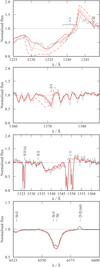 |
Fig. 8 Spectral observations of wind lines of SSN 13, normalised and compared to various models. The observed spectra of SSN 13 is shown by black line. Synthetic spectra with |


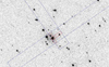 |
Fig. 9 Area on the sky around SSN 14. Blue boxes show the approximate positions of the two G140L slits with 2″ widths, while red boxes show the position along the slit from where the spectra of SSN 14 were extracted. Background is the F225W HST image, flux is log scaled. |
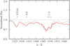 |
Fig. 10 Spectral observations of wind lines of SSN 14, normalised and compared to various models. The observed spectra of SSN 14 is shown by black line. Synthetic spectra with |


4.1.6 SSN 15 (MPG 368)
Bouret et al. (2003) assign this star the spectral type of O4–5 V((f*)). Rotational broadening, v sin i = 58 km s−1 is from Dufton et al. (2019). From our MUSE observations, we find T* = 40 kK and log g = 4.0. This temperature is similar to that found by Bouret et al. (2003), however they find a lower log g = 3.75. To reproduce the minimal emission in N iii λλ 7105, 7111, 7123 seen in the MUSE spectra, we reduce the temperature to T* = 39 kK and hence avoid this line emission produced in all hotter models.
We adopt an abundance of N/N⊙ = 0.6, in agreement with Bouret et al. (2003). This produces the best fit for N iii λλ 1183, 1185, N iv λ 1189, and N iv λ 1718 in the UV, in addition to showing emission in N iii λλ4634, 4641. All other lines are best fit with the abundances used in the grid models, as detailed in Table 3.
We find the best matching wind parameters of  , β = 1.0, D = 20, and v∞ = 2100 km s−1 (Fig. 11). This mass-loss rate is lower than
  , reported by Bouret et al. (2003). Similar to Bouret et al. (2003), for measuring wind parameters we exclude the NAC within the N v and C iv absorption troughs.
4.1.7 SSN 17 (MPG 396)
The spectral type of O7 V has been assigned by Massey et al. (1989). From our MUSE observations log g = 4.0 and T* = 37 kK. Dufton et al. (2019) gives v sin i = 196 km s−1 based on the He i λ 4471 line. There is no evidence for CNO enrichment in the MUSE observations so we adopt the grid abundances.
The C iv λλ 1548.2, 1550.8 wind profile is not seen in the UV spectra. A slight blueward asymmetry is evident in the N v λλ 1238.8, 1242.8 profile. This is confirmed by the comparison to a model with lower mass-loss rate ( ) which featured no synthetic blueward asymmetry (Fig. 12). A model with D = 10 could not replicate this lack of C iv λλ 1548.2, 1550.8 wind profile along with the slight observed N v λλ 1238.8, 1242.8 wind profile, so instead D = 1 (homogeneous winds) and D = 5 models were tried. The best fit wind parameters were therefore D = 1,
  , and v∞ = 1000 km s−1.
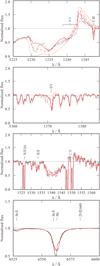 |
Fig. 11 Spectral observations of wind lines of SSN 15, normalised and compared to various models. The observed spectra of SSN 15 is shown by the black line. Synthetic spectra with |


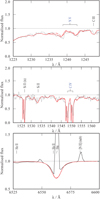 |
Fig. 12 Normalised spectral observations of wind lines of SSN 17, normalised and compared to various models. The observed spectra of SSN 17 is shown by the black line. Synthetic spectra with |


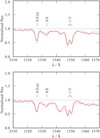 |
Fig. 13 Two seperate normalised spectral observations of the C iv λλ 1548, 1551 wind lines of SSN 18, normalised and compared to various models. The observations are shown by the black lines. Red lines are models. Top panel: high resolution E140M observations of SSN 18 (obtained on 28-09-2000) compared to a model with |


4.1.8 SSN 18 (MPG 487)
The spectral type O8 V is from Bouret et al. (2003) who analysed the echelle E140M high resolution UV spectrum. Dufton et al. (2019) provide v sin i = 131 km s−1 from He ii λ 4921. In the E140M spectrum, the wind profile in the N v λλ 1238.8, 1242.8 line is only marginally seen while there is no wind profile in C iv λλ 1548.2, 1550.8. Bouret et al. (2003) model the UV spectra with a homogeneous wind (D = 1) and derive  with an upper limit on v∞ ≤ 1500 km s−1.
We find that in our observations with G140L, the spectrum shows blueward absorption in the C iv λλ 1548.2, 1550.8 wind line (Fig. 13). Our G140L spectrum gives the same luminosity as the E140M spectra, showing there is no contamination in our G140L observation. This is also shown by an inspection of the F225W HST image which reveals no sources along the extraction of the G140L spectrum that could cause this feature through contamination.
By fitting the C iv λλ 1548.2, 1550.8 wind profile in the G140L spectra we find  , β = 0.8, v∞ = 1500km s−1. Density contrast D = 5 is needed to match the N v λλ 1238.8, 1242.8 wind lines simultaneously with the C iv λλ 1548.2, 1550.8 line. Keeping all other wind parameters constant and only varying the mass-loss rate, we adjust the model to produce synthetic spectra to fit the lack of C iv λλ 1548.2, 1550.8 wind profile in E140M spectra with
  , that is, a factor of ~4.5 lower mass-loss rate. This variability is discussed further in Sect. 5.3.
4.1.9 SSN 22 (MPG 476)
Spectral type of O6 V is determined in this work. Our MUSE observations give log g = 4.0 and T* = 38 kK. Dufton et al. (2019) derive v sin i = 100 km s−1 from He ii λ4921 line. Similar to SSN 14, this target has a very weak blueshifted absorption in C iv λλ 1548.2, 1550.8 extending to 1600 km s−1. There is a very slight N v λλ 1238.8, 1242.8 wind profile but a model with a smooth wind (D = 1) gives a synthetic profile that is too strong in N v λλ 1238.8, 1242.8 while the assumed clumped wind with D = 10 does not produce a strong enough synthetic profile. A density contrast of D = 5 along with the other wind parameters of  , β = 1.0, v∞ = 1600 km s−1 is required to match the UV and Hα observations.
4.1.10 SSN 31 (MPG 417)
SSN 31 has a spectral type O7.5 Vz which is determined in this work. We adopt v sin i = 98 km s−1 from Dufton et al. (2019). As with other mid-O type stars in our sample, no wind profiles are seen in the UV spectra with the exception of C iv λλ 1548.2, 1550.8 which shows a very slight blue-ward asymmetry, in this case up to 1000 km s−1. The observed spectrum is reproduced by a model with  , β = 1.0, and v∞ = 1000 km s−1. There is a marginally discernible NV λλ 1238.8, 1242.8 wind profile, and a density contrast of D = 10 fits both N v λλ 1238.8, 1242.8 and the Hα absorption well.
4.2 Scaling between mass-loss late and luminosity
Using spectral analyses we determined the stellar wind parameters for eighteen stars. In order to investigate how mass-loss rates depend on luminosity, we perform a power-law fit restricted to the stars with luminosity class V and Vz.
Stars within the sample with spectral types later than O7-8 (log L/L⊙ ≲ 5.0) do not show clear evidence of stellar winds, with the exception of a blueward absorption asymmetry in the C iv λλ 1548.2, 1550.8. Therefore, we were only able to derive an upper limit for their mass-loss rate and they were excluded from the fit. Additionally, we excluded SSN 18 due to its strong wind variability (see Sect. 5.3). The resulting fit yields  and is shown in Fig. 14.
In Fig. 14, theoretically predicted mass-loss rates of various authors are shown for comparison. It is evident that the recipe of Vink et al. (2000, 2001), which is most commonly used in stellar evolutionary models, overestimates the empirically found mass-loss rates. The more recent mass-loss prescription of Krtička & Kubát (2018) yield somewhat lower mass-loss rates but are still overestimating our results. The predictions of Björklund et al. (2021) are closest to our findings, even though they overestimate the mass-loss rates of the least luminous stars in our sample.
In order to make our results easier to compare to theoretical prescriptions, we employed a modified wind momentum diagram (see Fig. 15). The modified wind momentum is defined as  and the wind-momentum luminosity relation (WLR) at a given metallicity can be expressed as a power-law of the form.
 (4)
(4)
where x is the slope of our WRL and Do is the effective number of lines contributing to the wind acceleration and can be seen as a metallicity dependent offset. According to the theoretical predictions of Vink et al. (2000, 2001) the Galactic, LMC, and SMC WLR all should have a slope of x = 1.83 and offsets of Do = 18.68, 18.43, and 18.11, respectively. Observational studies of stars in the Galaxy (Repolust et al. 2004) and the LMC (Mokiem et al. 2007; Ramachandran et al. 2018) agree with these theoretical WLRs.
Shown in Fig. 15 and discussed in detail in Sect. 5.2, we find for our sample of O stars in the SMC follow a somewhat steeper WLR than the Vink et al. (2000, 2001) gradient of x = 1.83;
 (5)
(5)
Recent theoretical predictions of Björklund et al. (2021) are in much better agreement with our empirically found mass-loss rates than those of Vink et al. (2000, 2001). However we find that these predictions have a higher Dmom than we measure. By finding a steeper relation at lower Z, we support the Björklund et al. (2021) addition change from  to
to  such that the exponent α is proportional to L. Following this idea, we find
 (6)
(6)
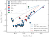 |
Fig. 14 Mass-loss rate as a function of stellar luminosity for the analysed O stars in NGC 346. Luminosity classes are distinguished by different colours as given in the legend. A power-law fit to the empirical results is represented by the blue solid line (see Sect. 4.2 for details). For comparison, we include stars with |


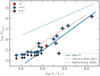 |
Fig. 15 Modified wind momentum Dmom as a function of luminosity. Legend as Fig. 14. The WLR to the empirical results is represented by the blue solid line. For comparison, theoretical WLR predictions from Vink et al. (2000, 2001) are included for the SMC (dashed blue line) and the theoretical predictions from Björklund et al. (2021) with comparable metallicity (dashed red line). |
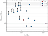 |
Fig. 16 Ratio of theoretical |


4.3 Wind line variability
Multi-epoch observations are available for six objects. Three stars, SSN 14 (O8 V), SSN 17 (O7 V), and SSN 57 (O9.5 V), are late O types and have no significant wind lines. Three stars, SSN 13 (O6 V), SSN 15 (O6 V), and SSN 18 (O8 V), display line variability (Fig. 17). The strongest line variability can be seen in SSN 18, which has one of the latest spectral types showing wind lines.
Although our sample is small, we tentatively conclude that all stars with wind features in their spectra display spectral variability. This is further discussed in the Sect. 5.3.
4.4 Ionising and mechanic energy feedback
The hydrogen ionising photon rates (QH) of each star are obtained from its best fitting PoWR model and are listed in Table B.1. Figure 18 shows log QH of our sample of O stars against spectral type. Previous studies have identified three slopes in this relation; one for O types, another for early B types and a third for types later than B2. In our sample, the relation between spectral type and ionising photon rate is given by log QH = 50.5 – 0.28 × ST, where ST refers to the subtype (e.g. 4 = O4). This relation is in line with the result by Ramachandran et al. (2019). A full table of the ionisation photon rates of the models used for our objects is presented in Appendix B.
From our models we find that, the feedback through ionising radiation in NGC 346 is dominated by SSN 9, which accounts for approximately 49% of the H ionising flux, 71% of the He i ionising flux and 99% of the He ii, with no other object in our sample offering any significant contribution to this. This ionising flux is six times greater than the contribution of the next most ionising object, SSN 13. We note that the binary system SSN 7, which was not part of this study, likely contains two early type stars which might be significant contributors of additional ionising flux. Nevertheless, we believe that SSN 9 dominates the ionising flux production which is supported by the morphology of the N 66 H ii region seen in the HST images (see top panel in Fig. 1 and Geist et al. 2022). The prominent, crescent structure tracing the photo-dissociation region has SSN 9 in the centre.
5 Discussion
5.1 Impact of model assumptions
We make multiple assumptions within the fitting process to save computational time and for consistency when analysing different stars from the same cluster. The stellar parameters are determined from a grid with the coarseness of 1000 kK in T* and 0.2 dex in log g. In addition, we assume turbulent velocity dependence upon spectral type, as well as constant Galactic extinction and abundances for all our sample stars. We vary abundances only when there is clear spectroscopic evidence of CNO enrichment. In this work we neglect the influence of intrinsic X-ray emission from stellar winds, which likely affect the N v wind lines.
In this work, the stellar wind inhomogeneity is treated using filling factor or ‘microcluming’ approximation (see Sect. 3.3). On the other hand, the strengths of resonance UV lines, and, correspondingly, derived  are affected by the porosity (or ‘macroclumping’ effects) (Oskinova et al. 2007). Using their 2D models, Sundqvist et al. (2010) examined in detail previous suggestions that the strongly non-monotonic wind velocity developing in 1D hydrodynamic simulations could lead to a reduction of the resonance line strength that is insensitive to spatial scales (this effect is sometimes dubbed ‘vorocity’). However, the full 3D radiative transfer models revealed that vorocity has only moderate effect on the UV resonance lines (Šurlan et al. 2012).
The clumping factors derived for some of our sample stars are high, implying that the porosity effects likely play a role in the resonance line formation. We computed a series of models which include porosity effects in both density and velocity, resulting in the increase of the empirically derived mass-loss rates. These will be a subject of our forthcoming publications.
Despite the assumptions made, the difference in the key parameters used for our results, log (L/L⊙) and  between our results and the results in the literature are minor, as shown in Table 6. The only significant difference is our model for SSN 13 demonstrates the difference that can result from a discrepancy in log g as small as 0.2. For SSN 9, while we find a different N and O abundance and a significantly different D, but the final mass-loss rate we find is very similar to that found by Bouret et al. (2013).
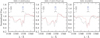 |
Fig. 17 Normalised spectra of C iv λλ 1548.2, 1550.8 wind lines in SSN 13, SSN 15, and SSN 18 (from left to right) taken at two different epochs shown by black and red lines. All spectra are convolved with G140L resolution (see text for details). Variability in the wind lines is clearly seen. |
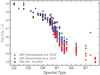 |
Fig. 18 Ionising photon rate as a function of stellar spectral type. The NGC 346 stars are shown by black diamonds. For comparison, the SMC stars analysed by Ramachandran et al. (2019) are included (red triangles) as well as LMC stars from Ramachandran et al. (2018) (blue circles). |
Comparison of parameters for the stars analysed by Bouret et al. (2013) using the cmfgen code (Hillier & Miller 1998) and for the stars in our sample analysed using the PoWR code (see text on the discussion of model assumptions)
5.2 Metallicity dependency and differences between derived mass-loss rate and theoretical predictions
We empirically derive a steeper WLR than predicted theoretically. The previous empirical study by Mokiem et al. (2006) found rough agreement with the theoretical predictions of Vink et al. (2000, 2001) but their WLR was based on Hα line fitted by smooth wind models in case of dwarf stars and overestimated M for these objects. Martins et al. (2004, 2005) find a breakdown of the WLR below log (L/L⊙) ≥ 5.4; we do not replicate this result (see Fig. 15).
Mokiem et al. (2006) showed that the Vink et al. (2000, 2001) theoretical  predictions do match stars with log L/L⊙ ≥ 5.8 (
 ). We only have one star, SSN 9, with this high luminosity. Using the theoretical mass-loss recipe of Vink et al. (2000, 2001) the star should have a mass-loss rate of
  , which is a factor of ten higher compared to our value. Our sample does not contain enough objects of sufficiently high luminosity to validated the Vink et al. (2000, 2001) relation in this range. Thus we are unable to explore if this discrepancy is also linked to the wind-metallicity relation as it is described above.
The main reason of our steeper WLR result is the accurate determination of the stellar wind properties of a large sample of low metallicity stars with luminosities below log L/L⊙ < 5.8. From the WLR at different metallicities (Galactic, LMC, and SMC), the wind-metallicity relationship ( ) is derived. We followed the idea of Björklund et al. (2021) and found that α ∝ L−1.2 (see Eq. (6)). This is a much stronger than α ∝ L−0.32 predicted by Björklund et al. (2021) and this is reflected in our steeper WLR.
5.3 UV wind profile variation and large scale wind structure
Similar their Galactic counterparts, the winds of low Z O stars are variable (Massa et al. 2000). The multi-epoch observations available for some of our sample stars allow us search for the variability in the wind lines and discuss its nature. SSN 18 (O8 V) shows the strongest wind line variability for any star in sample. Comparing the G140L spectrum (lower panel, Fig. 13) to the E140M spectrum (upper panel, Fig. 13) one can see that the C iv λλ 1548.2, 1550.8 blueward asymmetry is no longer detected. Bouret et al. (2003), who previously studied this object, only had access to the E140M spectrum without the C iv λλ 1548.2, 1550.8 line and so report an upper limit to  and v∞ based on the N v λλ 1238.8, 1242.8 asymmetry.
The differences between the mass-loss rates derived of these two observations is a factor of ~4.5. We speculate that the observed variability may be an extreme form of co-rotating interaction regions (CIRs), with no observable wind in the unstructured part of the wind and a C iv λλ 1548.2, 1550.8 wind profile only visible during the part of the rotation phase where the structured part of the wind is in our line of sight. Neither synthetic wind profile can be described as the upper limit on  , as we have no information about the phase of the variability and its links with rotation. A time series of observations are hence required to reliably measure the average
  .
.
Overall, we find a high occurrence of variability in the C iv λλ 1548.2, 1550.8 wind profile for the majority of the NGC 346 O6V-O8 V stars in our sample (see Fig. 17). Multi-epoch observations of SSN 9 suggest for the first time the presence of a structure moving blueward through the absorption trough of the wind line profile in low Z O star (see Fig. 7). More extensive time coverage is needed to identify whether these features are DACs repeating on the stellar rotation timescale and hence could be explained as originating in CIRs, by analogy with the Galactic objects (Massa & Prinja 2015).
Beside SSN 9, we find strong evidence of a DAC and we show the presence of NACs in the wind lines of SSN 13 and 15. We may be also observing a NAC in the C iv λλ 1548.2, 1550.8 absorption trough in SSN 11. Among all objects with available high resolution E140M or G140M spectra, only SSN 17 and 18 do not show DACs or NACs. However, SSN 17 has only very weak wind with low velocity (1000 km s−1) while SSN 18 shows the largest variation in its wind profiles at different epochs (see Sect. 4.3).
To summarise, whenever the spectral resolution is sufficient and the wind lines are broad, we do observe the presence of narrow discrete absorption features, commonly explained by the large-scale structures in stellar winds. If this property is found to be common across all massive stars at low metallicity, then spectroscopic analysis with the non-LTE codes that assume spherically-symmetric expansion, stationary, and allow only for a small scale inhomogeneities (clumping), are likely to underestimate  from stars with dense, co-rotating structures within the wind.
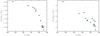 |
Fig. 19 Ratio of He i to H (left panel) and He ii to H (right panel) ionising photons of individual stars in our sample as functions of T*. |
5.4 Empirical Hertzsprung-Russell diagram
We construct an empirical upper Hertzprung–Russell diagram of the SMC where we include our new result on O stars in the NGC 346 cluster (Fig. 20). NGC 346 is commonly given the age ~3 Myr, while recent survey analysis by Dufton et al. (2019) suggest that NGC 346 is undergoing continuous star formation. The absence of O stars close to the Zero Age Main Sequence (ZAMS) is prominent. Stars with luminosity class Vz are present yet they appear to the right of the 3 Myr and later isochrones. The newly classified SSN 31 O7.5 Vz appears on the 5 Myr isochrone.
The absence of O stars close to the ZAMS in the Galaxy has previously been noted (Garmany et al. 1982; Herrero et al. 1992, 2007; Repolust et al. 2004; Castro et al. 2014; Holgado et al. 2018, 2020). This absence has also been noticed for the Magellanic Clouds (Massey et al. 1995b; Sabín-Sanjulián et al. 2014) and other galaxies in the Local Group (Massey & Johnson 1993; Massey et al. 1995a). This may be a result of lower accretion during star formation ( ) for objects more massive than 25 M⊙. This results in the birthline being to the right of the ZAMS (Holgado et al. 2020). An alternative explanation is that fast rotating massive stars evolve on a different track due to mixing (Maeder 1987). However, the threshold rotation velocity for this is far above v sin i for any of the massive stars in our sample as well as in Ramachandran et al. (2019).
In addition to SSN 9 and SSN 15, whose luminosity and temperature has been determined by Bouret et al. (2003), we derive the stellar parameters for SSN 13 and SSN 14, adding to the upper part of the HRD. If we consider the commonly adopted age of NGC346 (~3 Myr), all of our objects are to the right of the 3 Myr isochrome except for SSN 9, (O2 III(f*)).
6 Conclusions
In this work we systematically and consistently analysed the UV spectra complemented by the optical spectra for the nearly complete sample of O-type stars in the most massive young cluster, NGC 346, in the SMC galaxy at the metallicity Z = 1/7 Z⊙. We find that the empirically derived mass-loss rates of O type non-supergiant stars are significantly below the theoretical expectations of Vink et al. (2000, 2001). The later the spectral subtype the stronger is the discrepancy between the observed and predicted mass-loss rate. Accounting for binarity, wind porosity, and large-scale wind structure in empirical spectroscopic mass-loss rate diagnostics may help to reduce the discrepancy but is unlikely to eliminate it.
Our results show that the empirical wind luminosity relation (WLR) shows a steeper gradient than the theoretical predictions from Vink et al. (2000, 2001) and that recent theoretical WLRs produced by Krtička & Kubát (2018) and Björklund et al. (2021) for the SMC are in better agreement, but still underestimate our empirically derived gradient. We find, based on these observations and the best fit models, that the gradient of the WLR is dependent on Z. We find no indications of a break in the WLR around log L/L⊙ ~ 5.4 as suggested by Martins et al. (2004, 2005). For stars with log L/L⊙ < 5 only upper limits to  could be determined.
We find that the spectral type cutoff where later O types never have observable wind profiles in the UV is a lot later than previously reported. For stars with spectral type between O5 and O8 we find numerous objects with wind signatures in the UV spectra as well as those without. However, the wind signatures disappear in the UV spectra for stars later that O8-9 at the resolving power of STIS/G140L. In addition, our multi-epoch UV observations reveal that O stars at the SMC metallicity have variable winds. In one case, SSN 18, no wind profile is observable in one epoch and a strong profile appears in another. The common nature of such features suggests that winds of massive stars at low metallicity are highly structured.
We have resolved the core of the NGC 346 cluster and obtained the spectra of the nearly complete sample of O stars in this region. The empirical HRD shows a deficiency of the O type stars located at zero-age main sequence and in the upper part of the HRD, being in agreement with previous studies on the population of massive stars in the SMC. Our results highlight once more the deficiency of massive stars in this galaxy.
The ionising energy feedback in NGC 346 is dominated by the O2 giant SSN 9 which contributes ~49% of H ionising flux, 71% of He i ionising flux, and 99% of He ii ionising flux, though we note that the components of the SSN 7 binary are likely to be additional significant contributors to ionising flux based on their spectral type. We suggest that SSN 9 is largely responsible for the morphology of the H ii region seen in the HST images.
To summarise, our new in-depth study of the most massive young star cluster in the SMC galaxy, NGC 346, enabled by the UV spectroscopic capabilities of HST, resulted in the identification of eight new O-type stars in the cluster core, has enabled the measurement of wind properties of 19 O stars, and highlighted the key role O stars play in the ecology of young star clusters at low Z.
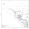 |
Fig. 20 Hertzsprung-Russell diagram for massive stars in the SMC. The objects of NGC 346 studied in this work are shown as diamonds. For completeness, SMC stars from Ramachandran et al. (2019) are illustrated as circles. Objects with luminosity class Vz are indicated by red colour. Solid lines are evolutionary tracks at SMC metallicity (Brott al. 2011), dotted lines are isochrones with Z = 0.002 (Georgy et al. 2013). Isochrones and evolutionary tracks are for non-rotating stars. |
Acknowledgements
This research is based on observations made with the NASA/ESA Hubble Space Telescope obtained from the Space Telescope Science Institute, which is operated by the Association of Universities for Research in Astronomy, Inc., under NASA contract NAS 5-26555. These observations are associated with programmes GO 15112 (PI L. Oskinova), GO 15837 (PI L. Oskinova). GO 7437 (PI D. J. Lennon), GO 7667 (PI R. Gililand), GO 8629 (PI F. Bruhweiler), GO 16098 (PI J. Roman-Duval), and GO 12940 (PI P. Massey). MJR would like to thank Ian D. Howarth (UCL) for his helpful comments during the early stages of this work. This publication was has benefited from a discussion at a team meeting sponsored by the International Space Science Institute at Bern, Switzerland. AACS and VR acknowledge support by the Deutsche Forschungsgemeinschaft (DFG – German Research Foundation) in the form of an Emmy Noether Research Group (grant number SA4064/1-1, PI Sander). TS acknowledges funding received from the European Research Council (ERC) under the European Union’s Horizon 2020 research and innovation programme (grant agreement number 772225: MULTIPLES). DP acknowledges financial support by the Deutsches Zentrum für Luft und Raumfahrt (DLR) grant FKZ 50 OR 2005. YHC acknowledges the MOST grants 109-2112-M-001-040 and 110-2112-M-001-020.
Appendix A Observations
Observations list. Positions, other names, and observational material for the O stars analysed in this work.
Appendix B Ionising photon rate
NGC 346 is an open star cluster surrounded by a lot of ionised material. For completeness we list the amount of ionising photons (log Q) released by each individual target according to our favourite PoWR Model. The resulting ionising fluxes for H, He i and He ii are listed in Table B.1. We note, that in this work only stars without a visible companion in the observed spectrum are included and that one of the major contributors, SSN 7 (one of the earliest type binaries in NGC 346), is not included here.
Ionising photon rates for each O star within our sample of NGC 346 objects.
Appendix C Grid fit for temperature and surface gravity
The observed (MUSE) and synthetic spectra of those O-type stars for which T* and log g are determined by fitting a grid model. The wings of the He ii λ 4860 line are used for measuring log g while the other He i and He ii lines are used to constrain T*. An analysis of B stars will be presented in a subsequent paper (Rickard et al. in prep).
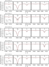 |
Fig. C.1 Synthetic Spectra Fitting to determine T* and log g. Red line: best fitted grid model; black line: observed MUSE spectrum. |
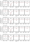 |
Fig. C.2 continued. |
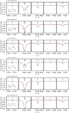 |
Fig. C.3 continued. |
Appendix D Spectral model fits
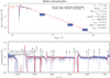 |
Fig. D.1 Spectral model fit of SSN 9. Top panel: SED fit of the model (red) to the flux calibrated observations of HST-STIS (blue). The blue squares with numbers mark the measure photometric data from Sabbi et al. (2007) which are used as additional constraints for the SED fit. Middle panel: Normalised HST-STIS spectrum (blue) overplotted by our synthetic spectrum (red). Lower panels: Same as the panel above, but now zoomed on the N v, O v and C iv UV resonance lines. |
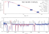 |
Fig. D.2 Same as Figure D.1, but for SSN 13. |
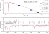 |
Fig. D.3 Same as Figure D.1, but for SSN 14. |
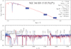 |
Fig. D.4 Same as Figure D.1, but for SSN 15. |
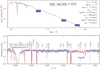 |
Fig. D.5 Same as Figure D.1, but for SSN 17. HST observations contains an error between approximately λ 1590Å and λ 1640Å due to insufficient overlap for correct concatenation. Left shown here for reference. Does not affect fit the quality of the fit due to absence of relevant lines in this region, |
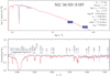 |
Fig. D.6 Same as Figure D.1, but for SSN 18. |
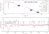 |
Fig. D.7 Same as Figure D.1, but for SSN 22. |
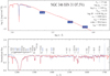 |
Fig. D.8 Same as Figure D.1, but for SSN 31. |
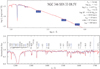 |
Fig. D.9 Same as Figure D.1, but for SSN 33. |
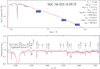 |
Fig. D.10 Same as Figure D.1, but for SSN 34. |
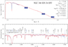 |
Fig. D.11 Same as Figure D.1, but for SSN 36. |
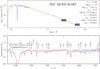 |
Fig. D.13 Same as Figure D.1, but for SSN 46. |
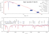 |
Fig. D.14 Same as Figure D.1, but for SSN 57. |
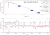 |
Fig. D.15 Same as Figure D.1, but for SSN 59. |
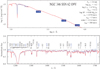 |
Fig. D.16 Same as Figure D.1, but for SSN 62. |
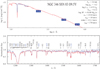 |
Fig. D.17 Same as Figure D.1, but for SSN 83. |
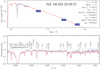 |
Fig. D.18 Same as Figure D.1, but for SSN 105. |
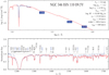 |
Fig. D.19 Same as Figure D.1, but for SSN 110. |
References
- Arias, J. I., Walborn, N. R., Simón Díaz, S., et al. 2016, AJ, 152, 31 [NASA ADS] [CrossRef] [Google Scholar]
- Björklund, R., Sundqvist, J. O., Puls, J., & Najarro, F. 2021, A&A, 648, A36 [EDP Sciences] [Google Scholar]
- Blair, W. P., Oliveira, C., LaMassa, S., et al. 2009, PASP, 121, 634 [NASA ADS] [CrossRef] [Google Scholar]
- Bodensteiner, J., Sana, H., Mahy, L., et al. 2020, A&A, 634, A51 [NASA ADS] [CrossRef] [EDP Sciences] [Google Scholar]
- Bouchet, P., Lequeux, J., Maurice, E., Prevot, L., & Prevot-Burnichon, M. L. 1985, A&A, 149, 330 [NASA ADS] [Google Scholar]
- Bouret, J. C., Lanz, T., Hillier, D. J., et al. 2003, AJ, 595, 1182 [NASA ADS] [CrossRef] [Google Scholar]
- Bouret, J. C., Lanz, T., Martins, F., et al. 2013, A&A, 555, A1 [NASA ADS] [CrossRef] [EDP Sciences] [Google Scholar]
- Brott, I., de Mink, S. E., Cantiello, M., et al. 2011, A&A, 530, A115 [NASA ADS] [CrossRef] [EDP Sciences] [Google Scholar]
- Castor, J. I., Abbott, D. C., & Klein, R. I. 1975, AJ, 195, 157 [NASA ADS] [CrossRef] [Google Scholar]
- Castro, N., Fossati, L., Langer, N., et al. 2014, A&A, 570, A13 [NASA ADS] [CrossRef] [EDP Sciences] [Google Scholar]
- Cignoni, M., Tosi, M., Sabbi, E., Nota, A., & Gallagher, J. S. 2011, AJ, 141, 31 [NASA ADS] [CrossRef] [Google Scholar]
- Conti, P. S., & Alschuler, W. R. 1971, ApJ, 170, 325 [NASA ADS] [CrossRef] [Google Scholar]
- Cranmer, S. R., & Owocki, S. P. 1996, ApJ, 462, 469 [NASA ADS] [CrossRef] [Google Scholar]
- Danforth, C. W., Sankrit, R., Blair, W. P., Howk, J. C., & Chu, Y.-H. 2003, ApJ, 586, 1179 [NASA ADS] [CrossRef] [Google Scholar]
- Dufour, R. J., Shields, G. A., & Talbot, R. J. J., 1982, ApJ, 252, 461 [NASA ADS] [CrossRef] [Google Scholar]
- Dufton, P. L., Evans, C. J., Hunter, I., Lennon, D. J., & Schneider, F. R. N. 2019, A&A, 626, A50 [NASA ADS] [CrossRef] [EDP Sciences] [Google Scholar]
- Evans, C. J., Lennon, D. J., Smartt, S. J., & Trundle, C. 2006, A&A, 456, 623 [CrossRef] [EDP Sciences] [Google Scholar]
- Garmany, C. D., Conti, P. S., & Chiosi, C. 1982, ApJ, 263, 777 [NASA ADS] [CrossRef] [Google Scholar]
- Geist, E., Gallagher, J. S., Kotulla, R., et al. 2022, PASP, 134, 064301 [NASA ADS] [CrossRef] [Google Scholar]
- Georgy, C., Ekström, S., Eggenberger, P., et al. 2013, A&A, 558, A103 [NASA ADS] [CrossRef] [EDP Sciences] [Google Scholar]
- Gouliermis, D. A., Chu, Y.-H., Henning, T., et al. 2008, ApJ, 688, 1050 [Google Scholar]
- Gräfener, G., Koesterke, L., & Hamann, W. R. 2002, A&A, 387, 244 [NASA ADS] [CrossRef] [EDP Sciences] [Google Scholar]
- Groenewegen, M. A. T., & Lamers, H. J. G. L. M. 1989, ApJS, 79, 359 [Google Scholar]
- Hainich, R., Rühling, U., Todt, H., et al. 2014, A&A, 565, A27 [NASA ADS] [CrossRef] [EDP Sciences] [Google Scholar]
- Hainich, R., Pasemann, D., Todt, H., et al. 2015, A&A, 581, A21 [NASA ADS] [CrossRef] [EDP Sciences] [Google Scholar]
- Hainich, R., Oskinova, L. M., Shenar, T., et al. 2018, A&A, 609, A94 [NASA ADS] [CrossRef] [EDP Sciences] [Google Scholar]
- Hainich, R., Ramachandran, V., Shenar, T., et al. 2019, A&A, 621, A85 [NASA ADS] [CrossRef] [EDP Sciences] [Google Scholar]
- Hamann, W. R., & Gräfener, G. 2004, A&A, 427, 697 [NASA ADS] [CrossRef] [EDP Sciences] [Google Scholar]
- Hamann, W. R., & Schmutz, W. 1987, A&A, 174, 173 [Google Scholar]
- Harries, T. J., Hilditch, R. W., & Howarth, I. D. 2003, MNRAS, 339, 157 [Google Scholar]
- Henize, K. G. 1956, ApJS, 2, 315 [CrossRef] [Google Scholar]
- Herrero, A., Kudritzki, R. P., Vilchez, J. M., et al. 1992, A&A, 261, 209 [NASA ADS] [Google Scholar]
- Herrero, A., Simon-Diaz, S., Najarro, F., & Ribas, I. 2007, in Massive Stars in Interactive Binaries, eds. N. St.-Louis, & A.F.J. Moffat, Astronomical Society of the Pacific Conference Series, 367, 67 [NASA ADS] [Google Scholar]
- Heydari-Malayeri, M., & Selier, R. 2010, A&A, 517, A39 [NASA ADS] [CrossRef] [EDP Sciences] [Google Scholar]
- Hilditch, R. W., Howarth, I. D., & Harries, T. J. 2005, MNRAS, 357, 304 [NASA ADS] [CrossRef] [Google Scholar]
- Hillier, D. J. 1987, ApJS, 63, 947 [NASA ADS] [CrossRef] [Google Scholar]
- Hillier, D. J., & Miller, D. L. 1998, AJ, 496, 407 [NASA ADS] [CrossRef] [Google Scholar]
- Holgado, G., Simón-Díaz, S., Barbá, R. H., et al. 2018, A&A, 613, A65 [NASA ADS] [CrossRef] [EDP Sciences] [Google Scholar]
- Holgado, G., Simón-Díaz, S., Haemmerlé, L., et al. 2020, A&A, 638, A157 [NASA ADS] [CrossRef] [EDP Sciences] [Google Scholar]
- Hony, S., Gouliermis, D. A., Galliano, F., et al. 2015, MNRAS, 448, 1847 [NASA ADS] [CrossRef] [Google Scholar]
- Hubeny, I., & Lanz, T. 1995, ApJ, 439, 875 [Google Scholar]
- Hubeny, I., Heap, S. R., & Altner, B. 1991, ApJ, 377, L33 [NASA ADS] [CrossRef] [Google Scholar]
- Hunter, I., Dufton, P.L., Smartt, S.J., et al. 2007, A&A, 466, 277 [NASA ADS] [CrossRef] [EDP Sciences] [Google Scholar]
- Kaper, L., Henrichs, H. F., Nichols, J. S., et al. 1996, A&AS, 116, 257 [NASA ADS] [CrossRef] [EDP Sciences] [Google Scholar]
- Kerton, C. R., Ballantyne, D. R., & Martin, P. G. 1999, AJ, 117, 2485 [Google Scholar]
- Krtička, J., & Kubát, J. 2018, A&A, 612, A20 [NASA ADS] [CrossRef] [EDP Sciences] [Google Scholar]
- Kudritzki, R. P., Cabanne, M. L., Husfeld, D., et al. 1989, A&A, 226, 235 [NASA ADS] [Google Scholar]
- Lamers, H. J. G.L.M., Snow, T.P., & Lindholm, D.M. 1995, AJ, 455, 269 [NASA ADS] [CrossRef] [Google Scholar]
- Larsen, S. S., Clausen, J. V., & Storm, J. 2000, A&A, 364, 455 [NASA ADS] [Google Scholar]
- Leitherer, C., Robert, C., & Drissen, L. 1992, AJ, 401, 596 [NASA ADS] [CrossRef] [Google Scholar]
- Lobel, A., & Blomme, R. 2008, ApJ, 678, 408 [NASA ADS] [CrossRef] [Google Scholar]
- Maeder, A. 1987, A&A, 178, 159 [NASA ADS] [Google Scholar]
- Martins, F., Schaerer, D., Hillier, D. J., & Heydari-Malayeri, M. 2004, A&A, 420, 1087 [NASA ADS] [CrossRef] [EDP Sciences] [Google Scholar]
- Martins, F., Schaerer, D., Hillier, D. J., et al. 2005, A&A, 441, 735 [NASA ADS] [CrossRef] [EDP Sciences] [Google Scholar]
- Massa, D., & Prinja, R. K. 2015, ApJ, 809, 12 [NASA ADS] [CrossRef] [Google Scholar]
- Massa, D., Fullerton, A. W., Hutchings, J. B., et al. 2000, ApJ, 538, L47 [NASA ADS] [CrossRef] [Google Scholar]
- Massey, P., & Johnson, J. 1993, AJ, 105, 980 [Google Scholar]
- Massey, P., Parker, J. W., & Garmany, C. D. 1989, AJ, 98, 1305 [Google Scholar]
- Massey, P., Armandroff, T. E., Pyke, R., Patel, K., & Wilson, C. D. 1995a, AJ, 110, 2715 [NASA ADS] [CrossRef] [Google Scholar]
- Massey, P., Lang, C. C., Degioia-Eastwood, K., & Garmany, C. D. 1995b, ApJ, 438, 188 [NASA ADS] [CrossRef] [Google Scholar]
- Massey, P., Zangari, A. M., Morrell, N. I., et al. 2009, ApJ, 692, 618 [Google Scholar]
- Massey, P., Morrell, N. I., Neugent, K. F., et al. 2012, ApJ, 748, 96 [NASA ADS] [CrossRef] [Google Scholar]
- Mokiem, M. R., de Koter, A., Evans, C. J., et al. 2006, A&A, 456, 1131 [NASA ADS] [CrossRef] [EDP Sciences] [Google Scholar]
- Mokiem, M. R., de Koter, A., Evans, C. J., et al. 2007, A&A, 465, 1003 [NASA ADS] [CrossRef] [EDP Sciences] [Google Scholar]
- Mullan, D. J. 1984, ApJ, 283, 303 [NASA ADS] [CrossRef] [Google Scholar]
- Nazé, Y., Hartwell, J. M., Stevens, I. R., et al. 2002, ApJ, 580, 225 [CrossRef] [Google Scholar]
- Niemela, V., & Gamen, R. 2004, New A Rev., 48, 727 [NASA ADS] [CrossRef] [Google Scholar]
- Niemela, V. S., Marraco, H. G., & Cabanne, M. L. 1986, PASP, 98, 1133 [NASA ADS] [CrossRef] [Google Scholar]
- Oskinova, L. M., Hamann, W. R., & Feldmeier, A. 2007, A&A, 476, 1331 [NASA ADS] [CrossRef] [EDP Sciences] [Google Scholar]
- Oskinova, L. M., Todt, H., Ignace, R., et al. 2011, MNRAS, 416, 1456 [NASA ADS] [CrossRef] [Google Scholar]
- Oskinova, L. M., Sun, W., Evans, C. J., et al. 2013, ApJ, 765, 73 [NASA ADS] [CrossRef] [Google Scholar]
- Pawlak, M., Soszyński, I., Udalski, A., et al. 2016, Acta Astron., 66, 421 [Google Scholar]
- Ramachandran, V., Hamann, W. R., Hainich, R., et al. 2018, A&A, 615, A40 [NASA ADS] [CrossRef] [EDP Sciences] [Google Scholar]
- Ramachandran, V., Hamann, W. R., Oskinova, L. M., et al. 2019, A&A, 625, A104 [NASA ADS] [CrossRef] [EDP Sciences] [Google Scholar]
- Reid, W. A., Payne, J. L., Filipović, M. D., et al. 2006, MNRAS, 367, 1379 [NASA ADS] [CrossRef] [Google Scholar]
- Repolust, T., Puls, J., & Herrero, A. 2004, A&A, 415, 349 [NASA ADS] [CrossRef] [EDP Sciences] [Google Scholar]
- Sabbi, E., Sirianni, M., Nota, A., et al. 2007, AJ, 133, 44 [NASA ADS] [CrossRef] [Google Scholar]
- Sabín-Sanjulián, C., Simón-Díaz, S., Herrero, A., et al. 2014, A&A, 564, A39 [NASA ADS] [CrossRef] [EDP Sciences] [Google Scholar]
- Sander, A., Shenar, T., Hainich, R., et al. 2015, A&A, 577, A13 [NASA ADS] [CrossRef] [EDP Sciences] [Google Scholar]
- Seaton, M. J. 1979, MNRAS, 187, 785 [NASA ADS] [Google Scholar]
- Shenar, T., Oskinova, L., Hamann, W. R., et al. 2015, ApJ, 809, 135 [Google Scholar]
- Simón-Díaz, S., & Herrero, A. 2014, A&A, 562, A135 [NASA ADS] [CrossRef] [EDP Sciences] [Google Scholar]
- Sohn, S. T., Azalee Bostroem, K., Proffitt, C., et al. 2019, Baltimore: STScI, 7 [Google Scholar]
- Sota, A., Maíz Apellániz, J., Walborn, N. R., et al. 2011, ApJS, 193, 24 [Google Scholar]
- Sundqvist, J. O., Puls, J., & Feldmeier, A. 2010, A&A, 510, A11 [NASA ADS] [CrossRef] [EDP Sciences] [Google Scholar]
- Šurlan, B., Hamann, W. R., Kubát, J., Oskinova, L. M., & Feldmeier, A. 2012, A&A, 541, A37 [NASA ADS] [CrossRef] [EDP Sciences] [Google Scholar]
- Trundle, C., Dufton, P. L., Hunter, I., et al. 2007, A&A, 471, 625 [NASA ADS] [CrossRef] [EDP Sciences] [Google Scholar]
- Vink, J. S., de Koter, A., & Lamers, H. J. G. L. M. 2000, A&A, 362, 295 [Google Scholar]
- Vink, J. S., de Koter, A., & Lamers, H. J. G. L. M. 2001, A&A, 369, 574 [NASA ADS] [CrossRef] [EDP Sciences] [Google Scholar]
- Walborn, N. R., & Blades, J. C. 1986, ApJ, 304, L17 [NASA ADS] [CrossRef] [Google Scholar]
- Walborn, N. R., & Fitzpatrick, E. L. 1990, PASP, 102, 379 [Google Scholar]
- Walborn, N. R., Lennon, D. J., Heap, S. R., et al. 2000, PASP, 112, 1243 [Google Scholar]
All Tables
Spectral types of O stars in this work, with references where drawn from published literature.
Minimum turbulent velocities (ξmin [km s−1]) adopted according to spectral type (Bouret et al. 2003).
Comparison of parameters for the stars analysed by Bouret et al. (2013) using the cmfgen code (Hillier & Miller 1998) and for the stars in our sample analysed using the PoWR code (see text on the discussion of model assumptions)
Observations list. Positions, other names, and observational material for the O stars analysed in this work.
All Figures
|
Fig. 1 NGC346 in the SMC. Top panel: optical colour composite of HST ACS image of the H ii region N 66, covering a total area of 3.5′ × 3.5v (≈62 pc × 62 pc at d = 61 kpc) on the sky. North is up, and east is to the left. The cluster of bright stars in the centre of the image is NGC 346. Credit: A. Nota (ESA/STScI). Lower panel: zoom to the region indicated by the green box in the top panel. The rectangles show our spectroscopic mosaic covering the central part of NGC 346. The GO 15112 STIS G140L slit positions are in red, while GO 8629 slit positions are in blue, see text for details. Background F225W image from HST archive (GO 12940). |
| In the text | |
|
Fig. 2 Normalised UV spectra of all identified O stars extracted within the G140L observations of both GO 15112 and GO 8629. |
| In the text | |
|
Fig. 3 Normalised MUSE spectra of all candidate OV-B0 V types stars in our sample. Black labels denote spectral types from literature. Red and bold labels denote spectral type assigned from this work. |
| In the text | |
|
Fig. 4 C ivλλ 1548.2, 1550.8 wind profile in the UV spectrum of SSN 31 (O7.5 Vz). Synthetic spectrum in red, observations in black. Top panel: synthetic spectrum with wind parameters v∞ = 1000 km s−1, β = 0.8, D = 10, and |
| In the text | |
|
Fig. 5 Example SED illustrating the method to estimate L and E(B−V). Spectrum and photometry (HST F225 W, F555W, and F814W) of SSN 36 are shown by blue line and boxes correspondingly. The best model, modified for extinction (Sect. 3.5), is in red. Model parameters are listed in the insert. |
| In the text | |
|
Fig. 6 Spectral observations of wind lines of SSN 9, normalised and compared to various models. The observed spectra of SSN 9 is shown by black line. Synthetic spectra with |
| In the text | |
|
Fig. 7 Multi-epoch observations of SSN 9 C iv λλ 1548.2, 1550.8 UV wind profile. Green line: observation taken on 22-11-2000. Blue and red lines: observations taken on 01-09-2020 and separated by ~1 h, with the blue-line spectrum observed prior to the red-line spectrum. Each of these exposures is ~40 min. A feature can be seen moving blueward on the timescale of hours. |
| In the text | |
|
Fig. 8 Spectral observations of wind lines of SSN 13, normalised and compared to various models. The observed spectra of SSN 13 is shown by black line. Synthetic spectra with |
| In the text | |
|
Fig. 9 Area on the sky around SSN 14. Blue boxes show the approximate positions of the two G140L slits with 2″ widths, while red boxes show the position along the slit from where the spectra of SSN 14 were extracted. Background is the F225W HST image, flux is log scaled. |
| In the text | |
|
Fig. 10 Spectral observations of wind lines of SSN 14, normalised and compared to various models. The observed spectra of SSN 14 is shown by black line. Synthetic spectra with |
| In the text | |
|
Fig. 11 Spectral observations of wind lines of SSN 15, normalised and compared to various models. The observed spectra of SSN 15 is shown by the black line. Synthetic spectra with |
| In the text | |
|
Fig. 12 Normalised spectral observations of wind lines of SSN 17, normalised and compared to various models. The observed spectra of SSN 17 is shown by the black line. Synthetic spectra with |
| In the text | |
|
Fig. 13 Two seperate normalised spectral observations of the C iv λλ 1548, 1551 wind lines of SSN 18, normalised and compared to various models. The observations are shown by the black lines. Red lines are models. Top panel: high resolution E140M observations of SSN 18 (obtained on 28-09-2000) compared to a model with |
| In the text | |
|
Fig. 14 Mass-loss rate as a function of stellar luminosity for the analysed O stars in NGC 346. Luminosity classes are distinguished by different colours as given in the legend. A power-law fit to the empirical results is represented by the blue solid line (see Sect. 4.2 for details). For comparison, we include stars with |
| In the text | |
|
Fig. 15 Modified wind momentum Dmom as a function of luminosity. Legend as Fig. 14. The WLR to the empirical results is represented by the blue solid line. For comparison, theoretical WLR predictions from Vink et al. (2000, 2001) are included for the SMC (dashed blue line) and the theoretical predictions from Björklund et al. (2021) with comparable metallicity (dashed red line). |
| In the text | |
|
Fig. 16 Ratio of theoretical |
| In the text | |
|
Fig. 17 Normalised spectra of C iv λλ 1548.2, 1550.8 wind lines in SSN 13, SSN 15, and SSN 18 (from left to right) taken at two different epochs shown by black and red lines. All spectra are convolved with G140L resolution (see text for details). Variability in the wind lines is clearly seen. |
| In the text | |
|
Fig. 18 Ionising photon rate as a function of stellar spectral type. The NGC 346 stars are shown by black diamonds. For comparison, the SMC stars analysed by Ramachandran et al. (2019) are included (red triangles) as well as LMC stars from Ramachandran et al. (2018) (blue circles). |
| In the text | |
|
Fig. 19 Ratio of He i to H (left panel) and He ii to H (right panel) ionising photons of individual stars in our sample as functions of T*. |
| In the text | |
|
Fig. 20 Hertzsprung-Russell diagram for massive stars in the SMC. The objects of NGC 346 studied in this work are shown as diamonds. For completeness, SMC stars from Ramachandran et al. (2019) are illustrated as circles. Objects with luminosity class Vz are indicated by red colour. Solid lines are evolutionary tracks at SMC metallicity (Brott al. 2011), dotted lines are isochrones with Z = 0.002 (Georgy et al. 2013). Isochrones and evolutionary tracks are for non-rotating stars. |
| In the text | |
|
Fig. C.1 Synthetic Spectra Fitting to determine T* and log g. Red line: best fitted grid model; black line: observed MUSE spectrum. |
| In the text | |
|
Fig. C.2 continued. |
| In the text | |
|
Fig. C.3 continued. |
| In the text | |
|
Fig. D.1 Spectral model fit of SSN 9. Top panel: SED fit of the model (red) to the flux calibrated observations of HST-STIS (blue). The blue squares with numbers mark the measure photometric data from Sabbi et al. (2007) which are used as additional constraints for the SED fit. Middle panel: Normalised HST-STIS spectrum (blue) overplotted by our synthetic spectrum (red). Lower panels: Same as the panel above, but now zoomed on the N v, O v and C iv UV resonance lines. |
| In the text | |
|
Fig. D.2 Same as Figure D.1, but for SSN 13. |
| In the text | |
|
Fig. D.3 Same as Figure D.1, but for SSN 14. |
| In the text | |
|
Fig. D.4 Same as Figure D.1, but for SSN 15. |
| In the text | |
|
Fig. D.5 Same as Figure D.1, but for SSN 17. HST observations contains an error between approximately λ 1590Å and λ 1640Å due to insufficient overlap for correct concatenation. Left shown here for reference. Does not affect fit the quality of the fit due to absence of relevant lines in this region, |
| In the text | |
|
Fig. D.6 Same as Figure D.1, but for SSN 18. |
| In the text | |
|
Fig. D.7 Same as Figure D.1, but for SSN 22. |
| In the text | |
|
Fig. D.8 Same as Figure D.1, but for SSN 31. |
| In the text | |
|
Fig. D.9 Same as Figure D.1, but for SSN 33. |
| In the text | |
|
Fig. D.10 Same as Figure D.1, but for SSN 34. |
| In the text | |
|
Fig. D.11 Same as Figure D.1, but for SSN 36. |
| In the text | |
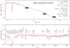 |
Fig. D.12 Same as Figure 1 |
| In the text | |
|
Fig. D.13 Same as Figure D.1, but for SSN 46. |
| In the text | |
|
Fig. D.14 Same as Figure D.1, but for SSN 57. |
| In the text | |
|
Fig. D.15 Same as Figure D.1, but for SSN 59. |
| In the text | |
|
Fig. D.16 Same as Figure D.1, but for SSN 62. |
| In the text | |
|
Fig. D.17 Same as Figure D.1, but for SSN 83. |
| In the text | |
|
Fig. D.18 Same as Figure D.1, but for SSN 105. |
| In the text | |
|
Fig. D.19 Same as Figure D.1, but for SSN 110. |
| In the text | |
Current usage metrics show cumulative count of Article Views (full-text article views including HTML views, PDF and ePub downloads, according to the available data) and Abstracts Views on Vision4Press platform.
Data correspond to usage on the plateform after 2015. The current usage metrics is available 48-96 hours after online publication and is updated daily on week days.
Initial download of the metrics may take a while.