| Issue |
A&A
Volume 664, August 2022
|
|
|---|---|---|
| Article Number | A84 | |
| Number of page(s) | 27 | |
| Section | Interstellar and circumstellar matter | |
| DOI | https://doi.org/10.1051/0004-6361/202142513 | |
| Published online | 10 August 2022 | |
The SEDIGISM survey: Molecular cloud morphology
II. Integrated source properties
1
Max-Planck-Institut für Radioastronomie,
Auf dem Hügel 69,
53121
Bonn, Germany
e-mail: This email address is being protected from spambots. You need JavaScript enabled to view it.
2
School of Physics & Astronomy, Cardiff University,
Queen’s Building, The Parade,
Cardiff
CF24 3AA, UK
3
Centre for Astrophysics and Planetary Science, University of Kent,
Canterbury
CT2 7NH,
UK
4
Laboratoire d’Astrophysique (AIM), CEA, CNRS, Université Paris-Saclay, Université Paris Diderot,
Sorbonne Paris Cité,
91191
Gif-sur-Yvette, France
5
Space Science Institute,
4765 Walnut St Suite B,
Boulder,
CO 80301, USA
6
School of Science and Technology, University of New England,
Armidale NSW
2351, Australia
7
I. Physikalisches Institut, Universität zu Köln,
Zülpicher Strasse 77,
50937
Cologne, Germany
8
Astrophysics Research Institute, Liverpool John Moores University, IC2,
Liverpool Science Park, 146 Brownlow Hill,
Liverpool,
L3 5RF, UK
9
Laboratoire d’astrophysique de Bordeaux, CNRS, Univ. Bordeaux,
B18N, allée Geoffroy Saint-Hilaire,
33615
Pessac, France
10
School of Physics and Astronomy, University of Exeter,
Stocker Road,
Exeter
EX4 4QL,
UK
11
Max-Planck-Institut für Astronomie,
Königstuhl 17,
69117
Heidelberg, Germany
12
Leibniz-Institut für Astrophysik Potsdam (AIP),
An der Sternwarte 16,
14482
Potsdam, Germany
13
INAF – Osservatorio Astronomico di Cagliari,
Via della Scienza 5,
09047
Selargius (CA), Italy
14
The American University of Paris,
2bis, Passage Landrieu
75007
Paris, France
Received:
22
October
2021
Accepted:
4
May
2022
Abstract
The Structure, Excitation, and Dynamics of the Inner Galactic InterStellar Medium (SEDIGISM) survey has produced high (spatial and spectral) resolution 13CO (2−1) maps of the Milky Way. It has allowed us to investigate the molecular interstellar medium in the inner Galaxy at an unprecedented level of detail and characterise it into molecular clouds (MCs). In a previous paper, we classified the SEDIGISM clouds into four morphologies. However, how the properties of the clouds vary for these four morphologies is not well understood. Here, we use the morphological classification of SEDIGISM clouds to find connections between the cloud morphologies, their integrated properties, and their location on scaling relation diagrams. We observe that ring-like clouds show the most peculiar properties, having, on average, higher masses, sizes, aspect ratios, and velocity dispersions, compared to other morphologies. We speculate that this is related to the physical mechanisms that regulate their formation and evolution; for example, turbulence from stellar feedback can often result in the creation of bubble-like structures. We also see a trend of morphology with the virial parameter, whereby ring-like, elongated, clumpy, and concentrated clouds have virial parameters in decreasing order. Our findings provide a foundation for a better understanding of MC behaviour, based on their measurable properties.
Key words: ISM: clouds / local insterstellar matter / ISM: bubbles / submillimeter: ISM
⋆ Member of the International Max Planck Research School (IMPRS) for Astronomy and Astrophysics at the Universities of Bonn and Cologne.
© K. R. Neralwar et al. 2022
 Open Access article, published by EDP Sciences, under the terms of the Creative Commons Attribution License (https://creativecommons.org/licenses/by/4.0), which permits unrestricted use, distribution, and reproduction in any medium, provided the original work is properly cited.
This article is published in open access under the Subscribe-to-Open model.
Open Access funding provided by Max Planck Society.
1 Introduction
Molecular clouds (MCs) are some of the densest and coldest regions in the interstellar medium (ISM) and the exclusive sites of star formation in galaxies (Dobbs et al. 2014; Heyer & Dame 2015; Miville-Deschênes et al. 2017). They are turbulent structures with masses of the order of 102–107 M⊙ and most of this mass is concentrated in high-mass giant molecular cloud complexes (>105 M⊙ for the Milky Way) (Roman-Duval et al. 2010). Generally speaking, most MCs are magnetically super-critical, though not by a large margin (Crutcher et al. 2010; Crutcher 2012; Dobbs et al. 2014). Moreover, magnetic fields vary from cloud to cloud, and some clouds may be magnetically supported (Chapman et al. 2011; Barnes et al. 2015). MCs span a range of sizes between ~ 1 and ~200 pc, and present a hierarchical structure with dense clumps and denser (proto-stellar or pre-stellar) cores (Blitz & Stark 1986; Rosolowsky et al. 2008; Ballesteros-Paredes et al. 2020). The surface densities of MCs have a wide range, in other words, ~1 to more than 1000 M⊙ pc–2 (Barnes et al. 2018). A typical value for the surface densities of clouds is ~100 M⊙ pc–2 (Roman-Duval et al. 2010; Rebolledo et al. 2012) and it may change with the Galactic environment (e.g. M51; Colombo et al. 2013; Sun et al. 2018).
The correlations between velocity dispersion and other cloud properties, such as surface density and the virial parameter, have led to various interpretations explaining their structure. The historically widely used Larson (1981) paper concluded that clouds are self-gravitating objects in virial equilibrium and the gravity acting on clouds is counterbalanced by internal forces, giving an average virial parameter around unity (Solomon et al. 1987; Fukui et al. 2008; Roman-Duval et al. 2010). Another work, Ballesteros-Paredes et al. (2011), argued that clouds are in free-fall collapse, but that the uncertainties and scatter in the size-linewidth relation allow for virial equilibrium to be a consistent mechanism. Field et al. (2011) present clouds as marginally self-gravitating pressure-confined objects. A more recent work, Vázquez-Semadeni et al. (2019), presents the global hierarchical collapse (GHC) scenario as a description of the processes involved throughout the life cycle of MCs, from their formation in the diffuse medium to their destruction by massive stars. It proposes a ‘moderated’ free-fall to maintain the cloud structure, which takes into account the interplay at different scales, and includes processes such as stellar feedback, which affect the overall cloud evolution.
The filamentary nature of MCs is ubiquitous in the Galaxy and most of the star-forming clumps are situated in large-scale filamentary structures (Schneider & Elmegreen 1979; Arzoumanian et al. 2011; Polychroni et al. 2013; Hacar et al. 2013; Li et al. 2016; Olmi et al. 2016; Kainulainen et al. 2017; Bresnahan et al. 2018; Mattern et al. 2018; Ballesteros-Paredes et al. 2020; Arzoumanian et al. 2022). The evolution of filaments is influenced by various mechanisms, such as ISM turbulence, shocked flows, supernovae feedback, or Galactic shear (Chen et al. 2020; Colombo et al. 2021). These filaments can be further classified into various types – for instance, bones or giant molecular filaments (GMFs) – based on their properties (e.g. aspect ratio; Zucker et al. 2018). The variations in filament properties might be a result of the Galactic environment and the scales at which they evolve. For example, recent studies attribute the formation of GMFs to galactic shear and large-scale gas motions, considering these filaments as a subset of giant MCs (Koda et al. 2006; Duarte-Cabral & Dobbs 2016).
The formation and evolution of MCs is still not completely understood (Ballesteros-Paredes et al. 2020). Similarly, there is no unique global property of MCs that can define their ability to form high-mass stars. Modern approaches towards studying MCs include an analysis of their three-dimensional structure (Zucker et al. 2021) and their morphological classification (Yuan et al. 2021) into filamentary and non-filamentary structures. Relating the cloud morphology to its properties and Galactic environment may provide us with a better understanding of MCs and star formation. It could also help us to understand the physical processes behind the structure of clouds (Arzoumanian et al. 2022).
Stellar feedback plays an important role in regulating the star formation in a galaxy and shaping the neighbouring MCs. Stars can impart mechanical energy in the form of turbulence, stellar winds and shocks, and radiative energy, which heats up the gas, leading to the creation and destruction of MCs and their substructures. Feedback drives the mass, energy, momentum, and metal enrichment into the surrounding ISM, inducing new star formation events (Ballesteros-Paredes et al. 2020; Schneider et al. 2020; Beuther et al. 2022). On the other hand, it can also shred the natal molecular gas, limiting further star formation (Geen et al. 2016; Urquhart et al. 2021). Feedback often results in the formation of interstellar bubbles (Deharveng et al. 2010; Jayasinghe et al. 2019), which are some of the most morphologically complex structures in the Galaxy. For instance, the bubble RCW 49 (Schneider et al. 2020; Rodgers et al. 1960) shows an expanding shell that is decoupled from the ambient ISM (Tiwari et al. 2021). Similarly, a fragmented ring of molecular gas is detected around the ionised region surrounding the bubble RCW 120 (Zavagno et al. 2007; Rodgers et al. 1960), the presence of which is attributed to the collect and collapse mode (Elmegreen & Lada 1977; Zavagno et al. 2006; Zhou et al. 2020; Luisi et al. 2021). These bubbles and shells are prime examples of the ring-like clouds discussed in this work.
In this paper, we try to find a connection between the morphology of MCs and their properties. The paper is organised as follows: Sect. 2 provides a brief overview of the survey data and the cloud catalogue used for the analysis. Section 3 gives a brief description of the methods used for the classification of clouds into different morphologies, and the resulting morphological classes and cloud samples. We have discussed these in detail in Neralwar et al. (2022, hereafter referred to as Paper I). In Sect. 4, we analyse the integrated properties of MCs for the four morphological classes. We also check if the results from the different cloud samples agree with each other for the different morphologies. In Sect. 5, we study Larson's and Heyer’s scaling relations, and in Sect. 6 we discuss the results and the physical processes leading to the observed morphologies. We summarise our main findings in Sect. 7.
2 Data
Structure, Excitation, and Dynamics of the Inner Galactic InterStellar Medium (SEDIGISM) is a southern hemisphere inner Galaxy survey that probes the moderately dense (≈103cm–3) ISM. It covers –60° ≤ l ≤ +18° and |b| ≤ 0.5° in several molecular lines, mainly the J = 2−1 transitions of 13CO and C18O. The observations for the survey were carried out using the 12m Atacama Pathfinder Experiment (APEX, Güsten et al. 2006) telescope. A detailed description of the observations, data reduction, and data quality checks is provided in Schuller et al. (2017) and Schuller et al. (2021).
Duarte-Cabral et al. (2021, hereafter called DC21), used the first data release (DR1; Schuller et al. 2021) of the SEDIGISM survey to obtain a catalogue of 10663 clouds using the scimes1 algorithm (detailed description in Colombo et al. 2015, 2019). The data have a full width at half maximum (FWHM) beam size of 28′′ with a 1 σ sensitivity of 0.8–1.0 K at 0.25 km s–1 spectral resolution. In Paper I, we classify these clouds based on their morphology (see Sect. 3) and thus add more information to the original catalogue2.
This cloud catalogue (hereafter called the SEDIGISM cloud catalogue) presents the directly measured properties and the derived properties for the clouds identified with scimes. Each cloud is assigned an ID from scimes and a name using its Galactic coordinates. The directly measured properties include the cloud’s position, velocity, velocity dispersion, and size, and the intensity associated with each cloud. The catalogue also lists near, far, and adopted kinematic distances to the clouds, their reliability and uncertainties, and the presence of star formation tracers. These properties were used to derive other properties such as the aspect ratio, mass, surface density, and the virial parameter. The catalogue also provides the values of the properties obtained after beam deconvolution, which are used in the current work.
3 Morphological Cloud Classification
We study the integrated cloud properties for different morphologies and this demands that the clouds be highly resolved and have reliable distance measurements. Thus, we use the clouds belonging to the science sample from DC21 to study their properties. The clouds in the science sample have reliable distance measurements, are well resolved (cloud area >3Ωbeam), and do not lie on the latitude edges of the survey (edge = 0; in the SEDIGISM catalogue).
Paper I presents the classification of MCs from the SEDIGISM cloud catalogue based on their morphology. It uses two methods for this: J plots (Jaffa et al. 2018) and by-eye (visual) classification. It is important to note that J plots is an automated algorithm that uses the principal moment of inertia of a structure to determine its morphology. It distinguishes the structures based on their degree of elongation and degree of central concentration, thus classifying them into three types: cores, filaments, and bubbles (rings). In Paper I, we also conducted a visual analysis of the integrated intensity maps of the clouds, which resulted in four morphological classes: (i) ring-like clouds (e.g. Fig. 1a), (ii) elongated clouds (e.g. Fig. 1b), (iii) concentrated clouds (e.g. Fig. 1c), and (iv) clumpy clouds (e.g. Fig. 1d). There are 298 clouds that could not be classified into any of the above classes.
The two classification methods were used to identify two samples from the SEDIGISM cloud catalogue. These are the visually classified (VC) and morphologically reliable (MR) samples. Both of these samples were obtained from the SEDIGISM full sample – a sample of 10663 MCs (detailed description in DC21). The VC sample was obtained by categorising the clouds into the four morphologies using by-eye classification (i.e. the SEDIGISM full sample excluding unclassified clouds), whereas the MR sample contains clouds that have the same morphology under both J plot and by-eye classifications. This means that the MR sample includes ring-like, elongated and concentrated clouds that are identified by J plots as bubbles, filaments, and cores, respectively. The clumpy clouds that are recognised as either filaments or cores by the J plots algorithm also belong to the MR sample. A detailed description of the classifications and the resulting samples is provided in Sects. 3 and 4.1 of Paper I.
We restrict our MR and VC samples in this paper (Table 1) to only the clouds from the science sample (DC21), and use this sub-sample of clouds for further analysis. These samples are used to understand the connection between cloud properties, their morphologies, and the effects of the Galactic environment. It is worth noting that the quality of classification for the MR sample is better than for the VC sample, as it is classified using both visual and automated classifications. However, this leads to the rejection of a large amount of data and results in a small sample size for some morphologies (e.g. ring-like clouds). In light of this, we use both samples3 for our analysis (Table 1).
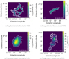 |
Fig. 1 Examples of different cloud morphologies. The images are integrated intensity (moment 0) maps of the 13CO (2−1) transition. The numbers in the right bottom corner of the images represent the J1 and the J2 moments (J plots algorithm), respectively. The colour bars represent the 13CO integrated intensity in K kms–1. The white contours represent the cloud edge. The white circles at the bottom left of the figures represent the telescope beam size. |
4 Results
In this section, we analyse the connection between cloud morphologies and their other properties, that is to say, cloud mass, surface density, radius, velocity dispersion, length, aspect ratio, and virial parameter. The properties used throughout this paper are the deconvolved properties from DC21. The cloud radius (effective radius and deconvolved radius) is calculated (in DC21) from the exact area of the cloud, assuming a spherical geometry. Therefore, the concept of radius may be inefficient in correctly describing the size of clouds with complex structures, which have a non-spherical geometry. An alternative measure of the major and minor axes of a cloud could be the length and width obtained using the geometric medial axis. The longest running central spine through a 2D projected cloud mask is considered to determine the cloud length, whereas the width is twice the average distance from the spine to the cloud edge. The cloud length (lengthMA) and the aspect ratio (ARMA) used in this work were obtained using the medial axis technique (DC21). The medial axis length is free of the assumption that clouds have a particular geometry and hence provides a different estimate of the cloud size (especially for elongated structures) compared to the cloud radius. Our implementation of the medial axis analysis does not consider the intensity distribution of the cloud, and therefore we do not trace the density-weighted spine.
The average integrated intensity of a cloud is obtained from the observed flux and is converted into the cloud mass M using the 13CO (2−1) to H2 conversion factor;  (Schuller et al. 2017). This mass is then used to obtain the surface density and the virial parameter for the clouds (DC21). The virial parameter is calculated assuming that clouds are spheres (Rosolowsky & Leroy 2006), but this is not consistent with the different cloud morphologies that we see. Moreover, the virial parameter is a crude property calculated using the balance between the kinetic and gravitational energies in the clouds, and might not be an accurate representation of the gravitational state of all the clouds. Nevertheless, we discuss it for the different morphologies as it is a widely used parameter in star formation literature (e.g. DC21).
The violin plots in Figs. 2–5 present distributions of the properties for the different cloud morphologies using the VC and MR samples. The main statistics (i.e. the median, interquartile range, skewness and kurtosis) of cloud properties for the different morphologies for both samples are reported in Table 2. The similar values (especially the medians) between the two samples, in most cases, indicate that they follow each other closely. The two samples show the most similar distributions for elongated and clumpy clouds (p-value = 1, Table A.1). The p-values presented throughout this work were obtained using the two sample Kolmogorov–Smirnov (KS) test. A detailed description of the KS test and p-values is presented in Appendix A. We compare the p-values between the VC and MR samples using the distributions of cloud properties in Table A.1. We find a p-value > 0.01 in ~85% of the cases, which suggests that the VC and MR samples usually show a similar distribution.
The differences between the distributions of the cloud properties for the various morphological classes can be identified visually from the violin plots (Figs. 2–5) and confirmed using the p-values from the KS test (Table A.2). The distributions for the different morphologies differ from each other for each cloud property (typically p-value < 0.01, Table A.2); for instance, the mass distribution of concentrated and ring-like clouds differ from each other.
Ring-like clouds show the most different properties compared to other morphologies. These clouds show higher average values and different distributions of radius, velocity dispersion, aspect ratio, and length, compared to other morphologies (Figs. 2 and 3; see ‘Median’ values in Table 2). They also have a higher average cloud mass than elongated and clumpy clouds, but the average surface density is comparable to elongated clouds and lower than the other morphologies (Fig. 4). Ring-like clouds also show slightly higher average values for the virial parameter compared to the other morphologies (Fig. 5). However, we again caution readers that the virial parameter might not correctly represent a cloud’s gravitational state for all the morphologies.
Concentrated clouds present a morphology quite different to ring-like clouds. These clouds have a high density at the centre, leading to a near-circular structure, and therefore exhibit smaller (average) lengths and aspect ratios (Fig. 3). They also have a lower average mass than other morphologies, but their small size results in a higher average surface density than other structures (Fig. 4).
Elongated clouds and clumpy clouds have comparable radius, velocity dispersion, length, and aspect ratio4 distributions (Figs. 2 and 3), with elongated clouds having more tailed distributions towards both the lower and higher values (see kurtosis in Table 2). The lower kurtosis of clumpy clouds may be a result of their smaller sample size. The length distributions (Fig. 3) of these two morphologies are similar to those of all clouds, which might be because most of the clouds have an elongated structure. Clumpy clouds have more mass but similar lengths to elongated clouds, resulting in higher surface densities (Fig. 4).
We also checked if the distribution of the clouds in the Galaxy is influenced by environmental factors, namely the Galactocentric radius/distance (Rgal) and the Galactic height (zgal (see Fig. 6). We did not find any specific environmental trend that separates a particular cloud morphology from others. All cloud morphologies show a Gaussian-like distribution in the Rgal histograms (Fig. 6, top). The small sample size at a smaller Rgal (Fig. 6; top) is due to the rejection of clouds near the Galactic centre (the science sample in DC21 excludes clouds with unreliable distances), whereas the small sample size at a higher Rgal (which for SEDIGISM corresponds to large heliocentric distances) is mostly due to the sensitivity and resolution limitations of the telescope. Unsurprisingly, a large number of MCs are situated at low Galactic heights (Fig. 6, middle), which may be a consequence of the high density of molecular gas in the Galactic plane. Moreover, all the morphologies seem to be distributed similarly across the Galactic height.
In order to identify any potential observational biases, we also investigated how the different morphologies are distributed as a function of heliocentric distance (Rd). The Rd histograms show that ring-like clouds have a higher concentration closer to us (Fig. 6; bottom). This could be due to a projection effect, leading to distortion in the observed structure of the clouds at large distances. Also, the most distant ring-like clouds could be unresolved and thus get classified into other morphologies. This is possibly reflected in the distribution of concentrated clouds, which shows slightly higher number densities at a larger Rd. Hence, this is most likely a consequence of observational bias and not a physical phenomenon. The distribution of other morphologies is similar along the heliocentric distance, with a dip in the number of clouds at Rd ≈ 6 kpc. The clouds in this region lie very close to the tangent velocity and are assigned a higher distance value (i.e. the tangent distance) to avoid distance ambiguity (see Sect. 4.1 in DC21).
We observed that clouds of all morphologies are abundant at all Rd (Fig. 6; bottom). However, the slight trends in the distributions indicate the presence of observational biases. We discuss the observational limitations that potentially affect our analysis in Appendix B. The influence of biases is most visible in the directly measured properties, namely mass, radius, and length. For example, smaller and less massive clouds can be detected in our vicinity, but the technical limitation of telescopes minimises their detection at large distances. We also discuss the influence of the environmental factors, that is Rgal and zgal, in Appendix C. We find that smaller clouds are usually seen at low Galactic heights. However, clouds at all Galactic heights show similar aspect ratios. A general observation is that the clouds’ properties follow the global trends (as seen in Figs. 2–5) irrespective of the Galactic environment and the observational biases.
Quantitative description of the clouds.
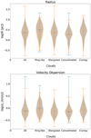 |
Fig. 2 Distribution of radius (top) and velocity dispersion (bottom) for the VC (blue) and MR (orange) samples. The violin plots present the density of the data at different values, which is smoothed through kernel density estimation. The horizontal lines at the ends and middle of the plots represent the extreme and the median values of the distributions, respectively. |
Statistics of integrated properties for various cloud morphologies.
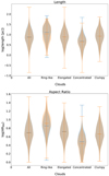 |
Fig. 3 Distribution of length (top) and aspect ratio (bottom). The symbols and conventions follow Fig. 2. |
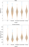 |
Fig. 4 Distribution of mass (top) and surface density (bottom). The symbols and conventions follow Fig. 2. |
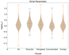 |
Fig. 5 Distribution of virial parameter for the VC and MR samples. The symbols and conventions follow Fig. 2. |
5 Scaling Relations
Larson’s size-linewidth relation (Larson 1981), also known as Larson’s first law, is one of the most studied scaling relations, which has provided observational constraints on the dynamics of MCs for the past 40 yr. The relation συ= 1.10 L0.38 was obtained by analysing a large number of MCs of different sizes, from subparsec-sized MCs to those measuring a few hundred parsecs. It has a similar form to Kolmogorov’s law for turbulence and implies that larger clouds have a higher velocity dispersion. It was further updated for MCs using analysis from Solomon et al. (1987), as discussed in Colombo et al. (2019).
We present the size-linewidth relation for the various cloud morphologies in Fig. 7. All cloud morphologies follow the general trend of high velocity dispersions for large clouds. However, it should be noted that the ‘size’ in terms of an equivalent radius is a better approximation for some clouds than others. The high values of velocity dispersion for ring-like clouds with large radii (log(R) > 0.5) might be attributed to the momentum imparted due to stellar feedback. A larger radius means that more of the gas (shell) has travelled farther away from the centre, resulting in a higher velocity difference between the centre and the edge. Although we expect the ring-like clouds to have a vertical offset given their higher velocity dispersions, this is not the case and they still lie along Larson’s relation (Fig. 7). We performed principal component analysis (PCA) for different cloud morphologies on the Larson’s plot (Fig. 7) to obtain the confidence ellipses (1–sigma) and compared the cloud distributions with the Larson’s relation. The slopes of the confidence ellipses for the clouds (Table 3) may indicate that elongated clouds and clumpy clouds (slope = 0.48) follow Larson’s first law (slope = 0.50) more closely than other morphologies. However, the large scatter in the data (Fig. 7) prevents us from confirming this.
Larson’s second relation correlates the velocity dispersion to cloud mass, implying that clouds are approximately in virial equilibrium, while the third relation shows the anti-correlation between cloud mean density and size. These relations, together with the analysis of Solomon et al. (1987), assert that clouds have a constant surface mass density. Heyer et al. (2009) reanalysed the clouds in the first quadrant of the Galaxy and found that these clouds do not have a constant surface mass density and they are not necessarily gravitationally bound. We show Heyer’s relation  for different cloud morphologies in Fig.8 and report the slopes of the corresponding 1-sigma PCA ellipses in Table 4. The different cloud morphologies show a trend with respect to the virial parameter, with ring-like clouds present towards a region of higher virial parameter. This is understood to mean that ring-like clouds are effectively expanding and thus not gravitationally bound. Towards a higher surface density and a lower velocity dispersion (i.e. a lower virial parameter), the regions are correspondingly occupied by elongated, clumpy, and then concentrated clouds. This is in agreement with our previous analysis of concentrated clouds being dense, gravitationally bound compact objects. We also observe that none of the cloud distributions follow αvir = 1 (Heyer et al. 2009), but the bulk of clouds could be virialised if they were under a relatively mild external pressure or were contracting at some fraction of free fall (Fig. 8).
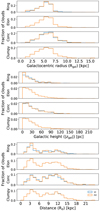 |
Fig. 6 Histogram (normalised) for distribution of clouds with respect to Galactocentric radius (top) Galactic height (zgal) (middle), and heliocentric distance (bottom). The histograms represent the ratio of clouds in each bin to the total number of clouds in all the bins. The bin width is 1 kpc for the heliocentric distance and Galactocentric radius plots, and 1 pc for the zgal histogram. Blue represents the VC sample and orange represents the MR sample. The cloud morphologies from top to bottom represent ring-like clouds (Ring), elongated clouds (Elon), concentrated clouds (Cone), and clumpy clouds (Clumpy). |
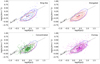 |
Fig. 7 Size-linewidth relation (συ versus R) using the MR sample. The dashed line represents Larson’s first relation (Larson 1981; Solomon et al. 1987). The different colours represent four cloud classes (Sect. 3); ring-like clouds are represented in blue, elongated clouds in red, concentrated clouds in green, and clumpy clouds in magenta. The contours include 68% of the data (1–sigma level) and the small circles represent centroids (means) of the distributions. The expected slope for the relation is 0.5 (dashed black line) (Larson 1981). |
Slopes and their standard deviations (SD) recovered from PCA on Larson’s scaling relation (συ ∝ Rslope) for the different cloud morphologies.
Slopes recovered from PCA on the Heyer scaling relation  .
.
6 Discussion
The differences in properties of different morphologies can be associated with various physical processes that play a role in the formation and evolution of clouds. The large size (as measured by the length and radius in Figs. 2 and 3) and aspect ratio (Fig. 3) for ring-like clouds can be attributed to their formation process. These clouds could be associated with infrared bubbles, which form due to stellar winds and radiation feedback. We find in Paper I that 605 ring-like clouds show association with infrared bubbles from the Milky Way Project (MWP). Stellar feedback could impart high velocity and turbulence to the shells, which then travel large distances to form large rings with high velocity dispersion (Snell et al. 1980; Liu et al. 2019). Ring-like clouds have the highest mass (on average). However, the large sizes of these clouds result in them having lower surface densities than other structures. Overall, ring-like clouds show the most extreme properties compared to the global distribution of clouds, as well as other morphologies.
The high mass and surface density (Fig. 4) of the clumpy clouds can be explained in two possible ways. The first hypothesis is that these are multiple overlapping clouds, considered to be a single cloud by scimes. The other hypothesis is that these clouds evolve similar to globular filaments (Schneider & Elmegreen 1979), having multiple dense regions in the filamentary structure. The second hypothesis is supported by higher star formation efficiencies (refer Paper I) for these clouds when compared to elongated clouds. Clumpy clouds have length distributions similar to elongated clouds, which could be due to a common formation or evolution mechanism, leading to filamentary structures of comparable sizes. It could also be an artefact of the cloud selection criteria used by the scimes algorithm, which is oriented towards selecting clouds with similar sizes and could thus present a single MC as smaller individual clouds, or combine small MCs and present them as a single cloud.
A major observation across all the data samples and throughout the different Galactic environments is that most of the MCs are elongated (Table 1; histograms in Figs. C.1, C.2, C.9, C.10, B.1 and B.2). The average properties of elongated clouds lie between those of ring-like clouds and concentrated clouds. The large sample size for elongated clouds might be the reason for their values being non-extreme. We also find that the Galactic environment does not significantly influence the trends in the integrated properties for most of the morphologies (see the ridge plots in Appendix B).
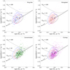 |
Fig. 8 Scaling relation between |

7 Summary
In this paper, we study the connection between the morphology of clouds and their integrated properties. We also analyse how the different cloud morphologies are distributed in the Galaxy. Our analysis is based on the catalogue of MCs from the SEDIGISM survey (presented in DC21; along with the integrated properties). Clouds were classified into four types based on their morphology (in Paper I). Our main findings are as follows:
Elongated clouds are the most abundant type of clouds in the Galaxy, with their average properties lying between ring-like and concentrated clouds;
Concentrated clouds have the smallest median sizes and highest median surface densities of all cloud categories;
Ring-like clouds show the most discrepant properties compared to the global population of clouds, with higher average mass, radius, length, aspect ratio, and velocity dispersion than other morphologies;
The different morphology classes are not distributed differently in terms of Galactocentric distance (Rɡal) and Galactic height (zgal);
The distributions of clouds do not show significant differences on Larson’s size-linewidth plot for the different morphologies;
Heyer’s scaling relation shows the evolution of morphologies with the virial parameter, with ring-like, elongated, clumpy, and concentrated clouds lying in order of decreasing virial parameter.
In conclusion, we find some connections between the integrated properties of the MCs and their morphology. The ringlike clouds show an extreme behaviour compared to other cloud morphologies, which may be a consequence of their nature, in other words, their formation due to stellar feedback. Moreover, the global trends in the properties for different morphologies are followed even in separate smaller regions of the Galaxy (i.e. throughout the distance bins (Appendix C)), irrespective of the observational biases (Appendix B). Even though we did not find any particular trend in the distribution of different types of clouds as a function of Galactocentric distances or Galactic height, we have not looked into other environments within the Galaxy, possibly more critical to the evolution of clouds, such as spiral arms or the Galactic centre. The categorisation of clouds into different morphologies could thus give way to various potential follow-up studies to help understand the role of the Galaxy in shaping the formation and evolution of MCs.
Acknowledgement
The authors thank the referee for their valuable comments on the draft, which helped improve the quality of the paper. This publication is based on data acquired with the Atacama Pathfinder Experiment (APEX) under programmes 092.F-9315 and 193.C-0584. APEX is a collaboration among the Max-Planck-Institut für Radioastronomie, the European Southern Observatory, and the Onsala Space Observatory. This publication uses data generated via the Zooniverse.org platform, development of which is funded by generous support, including a Global Impact Award from Google, and by a grant from the Alfred P. Sloan Foundation. A part of this work is based on observations made with the Spitzer Space Telescope, which is operated by the Jet Propulsion Laboratory, California Institute of Technology under a contract with NASA. K.R.N. thanks Henrik Beuther for the valuable suggestions and feedback on the paper. K.R.N. would also like to thank Antonio Hernandez for his careful reading of the manuscript. DC acknowledges support from the German Deutsche Forschungsgemeinschaft, DFG project number SFB956A. A.D.C. acknowledges the support from the Royal Society University Research Fellowship (URF/R1/191609). H.B. acknowledges support from the European Research Council under the Horizon 2020 Framework Programme via the ERC Consol-idator Grant CSF-648505. H.B. also acknowledges support from the Deutsche Forschungsgemeinschaft in the Collaborative Research Center (SFB 881) “The Milky Way System” (subproject B1). C.L.D. acknowledges funding from the European Research Council for the Horizon 2020 ERC consolidator grant project ICYBOB, grant number 818940.
Appendix A Kolmogorov?Smirnov test and p-value
The two-sample KS test is a non-parametric goodness-of-fit test that compares the cumulative distribution of two datasets by calculating the p-value and the maximum difference between them. We use the null hypothesis that the two distributions are obtained from the same distribution. Hence, a low p-value (typically below 0.01) leads to the rejection of the null hypothesis, and it is an indication that the two samples belong to different distributions. All the p-values throughout this paper were obtained from the KS test. We used the ks_2samp module from the python scipy package to implement the KS test on our distributions.
We used the KS test for two major tasks. The first was to confirm whether the distribution of the properties for a particular morphology is the same for the VC and MR samples. We confirm that the VC and MR samples are consistent with each other in Table A.1. The second task was to check if different morphologies show different distribution for a given property. The differences in the properties for the different morphologies can be visually distinguished in the violin plots (Fig. 3–5) and ridge plots (appendix B and C), and they are statistically confirmed in Table A.2.
P-values for the two-sample KS test conducted on the VC and MR samples for each property and morphology.
P-values for the two-sample KS test conducted on the different morphologies for each cloud property (VC sample).
Appendix B Testing the observational biases affecting cloud properties and morphological trends
The sensitivity and resolution limitations of the telescope may result in the incorrect classification of cloud morphology at large distances (Rd). We discuss the effects of these technical limitations in detail in this section using the ridge plots for heliocentric distance (Rd). In general, ridge plots are a visualisation tool that show the distribution of a numerical value for various groups. In our case, they can be considered violin plots for cloud properties in separate distance bins. The clouds are separated into nine distance bins with a 2 kpc width each, covering 0–18 kpc, based on their proximity to the Sun. Fig. B.1 shows the number of structures in each distance bin from 0–24 kpc.
The cloud properties that are most affected by the technical limitations are mass and size (radius and length). They show visible changes in the median as well as the distribution range across the distance bins. Fig. B.2 shows that the lower limit on mass increases with Rd. At a smaller Rd, low-mass clouds can be detected due to the high resolution and sensitivity of the telescope, but as Rd increases, the low-mass clouds are perceived as background noise. Similarly, we also find that the lower limit on radius (Fig. B.4) and length (Fig. B.8) increases with distance, following the same principle as mass distributions.
The surface density (Fig. B.3), aspect ratio (Fig. B.6), and velocity dispersion are not strongly affected by the technical limitations. The distributions for the virial parameter (Fig. B.7) show the most overlap compared to those of other properties. The decrease in the virial parameter with an increasing Rd can be attributed to observational biases at play (discussed in appendix C of DC2l).
We study the cloud properties in a two-dimensional positionposition space, and it could lead to the projection effects affecting our analysis. For example, our cloud length and width do not represent the original dimensions of the MCs, but rather a projected length and width. Similarly, the cloud morphology is also influenced by the positioning of clouds with respect to the telescope’s line of sight. However, given the large size of our data sample, the general trends in the results are unlikely to be affected, and thus we ignore the projection effects in this work.
It is interesting to note that, regardless of the changes in the properties with distance, the properties show similar trends across all the distance bins for the different morphologies. This validates our conclusions on the trends found for the full samples (see Sec. 4).
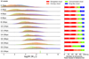 |
Fig. B.1 Mass ridge plot for the VC sample with Rd bins. |
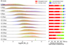 |
Fig. B.2 Mass ridge plot for the MR sample with Rd bins. |
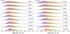 |
Fig. B.3 Surface density ridge plots with Rd bins. Left (solid): VC sample. Right (dashed): MR sample. |
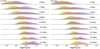 |
Fig. B.4 Radius ridge plots with Rd bins. Left (solid): VC sample. Right (dashed): MR sample. |
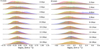 |
Fig. B.5 Velocity dispersion ridge plots with Rd bins. Left (solid): VC sample. Right (dashed): MR sample. |
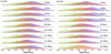 |
Fig. B.6 Aspect ratio ridge plots with Rd bins. Left (solid): VC sample. Right (dashed): MR sample. |
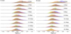 |
Fig. B.7 Virial parameter ridge plots with Rd bins. Left (solid): VC sample. Right (dashed): MR sample. |
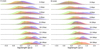 |
Fig. B.8 Length ridge plots with Rd bins. Left (solid): VC sample. Right (dashed): MR sample. |
Appendix C Dependence of cloud properties on the Galactic environment
The properties of MCs might show changes within different Galactic environments and based on their position in the Galaxy. We studied changes in the integrated properties of MCs based on their location in the Galaxy for the VC and MR samples using ridge plots. The data in each bin were plotted separately for each morphology in order to understand the environmental influence on each of the cloud properties for the different morphologies. The distributions of elongated clouds and clumpy clouds for the two samples are nearly identical as only a few of these clouds from the VC sample are not a part of the MR sample. The clouds are separated into distance bins based on two distance5 types. The first is the Galactocentric radius (Rgal), that is to say, the distance of a cloud from the centre of the Milky Way. The second is the Galactic height (zgal), in other words, the vertical height of a cloud from the Galactic plane. The cloud properties, namely mass, surface density, radius, velocity dispersion, aspect ratio, virial parameter, and length, were studied using ridge plots. The low sample size of morphologies in some bins led to sporadic peaks in the plots and also prohibited an in-depth study.
Appendix C.1 Galactocentric Radius (Rgal) Bins
This section presents the ridge plots with Galactocentric radius (Rgal) bins. The data are divided into eight bins of width 1 kpc from 2–10 kpc6. The central part of the Galaxy (< 1 kpc) is excluded because the local gas motions influence the overall properties, causing a change in the dynamics of the region. The decrease in sample size at a large distance from the Galactic centre sets an upper limit of 10 kpc for Rgal bins (Fig. C.1 and C.2).
The mass distribution for the two samples (Fig. C.1 and C.2) show the highest values for ring-like clouds and clumpy clouds. The surface density distributions (Fig. C.3) follow the global trends (Sec. 4), showing high values for concentrated and clumpy clouds. The properties pertaining to the size of the clouds show similar features across most of the Rgal bins. These are the radius (Fig. C.4) and length (Fig. C.8), which show the highest values for ring-like clouds. The aspect ratio distribution (Fig. C.6) also follows similar trends. These high values can be explained as a consequence of stellar feedback expanding the bubbles (see Sec. 6).
Appendix C.2 Galactic Height (zgal) Bins
In this section, we study the clouds by distributing them into zgal bins. The highest zgal value for the clouds is ≈ 230 pc, however, <1 % clouds lie above 160 pc. Thus, we binned the clouds into 8 bins of width 20 pc covering 0–160 pc. Clouds near the Galactic plane have a larger span of sizes (both radius and length), as seen in Figs. C.12 and C.16. Smaller clouds at higher Galactic heights might be obscured due to the foreground gas in the Galactic plane. The sensitivity and resolution of the telescope could also prevent the detection of smaller clouds at large distances. Clouds at all Galactic heights exhibit almost similar aspect ratio distributions (Fig. C.14), demonstrating that they show similar average shapes for a given morphology. We also see that less massive clouds are mostly located near the Galactic plane (Figs. C.9 and C.10). The virial parameter distribution has a mild trend, suggesting a lower average value with increasing Galactic height (Fig. C.15). To summarise, we detect a greater number of smaller and less massive clouds in the Galactic plane than at large Galactic heights, but this could be due to the foreground molecular gas, telescope limitations, or both.
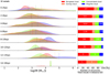 |
Fig. C.1 Mass ridge plot for the VC sample with Rgal bins. The vertical dashed lines represent the medians of the distributions. |
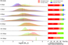 |
Fig. C.2 Mass ridge plot for the MR sample with Rgal bins. The vertical dashed lines represent the medians of the distributions. |
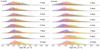 |
Fig. C.3 Surface density ridge plots with Rgal bins. Left (solid): VC sample. Right (dashed): MR sample. |
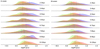 |
Fig. C.4 Radius ridge plots with Rgal bins. Left (solid): VC sample. Right (dashed): MR sample. |
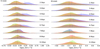 |
Fig. C.5 Velocity Dispersion ridge plots with Rgal bins. Left (solid): VC sample. Right (dashed): MR sample. |
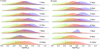 |
Fig. C.6 Aspect ratio ridge plots with Rgal bins. Left (solid): VC sample. Right (dashed): MR sample. |
 |
Fig. C.7 Virial Parameter ridge plots with Rgal bins. Left (solid): VC sample. Right (dashed): MR sample. |
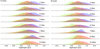 |
Fig. C.8 Length ridge plots with Rgal bins. Left (solid): VC sample. Right (dashed): MR sample. |
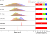 |
Fig. C.9 Mass ridge plot for the VC sample with zgal bins. |
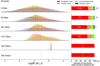 |
Fig. C.10 Mass ridge plot for the MR sample with zgal bins. |
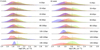 |
Fig. C.11 Surface density ridge plots with zgal bins. Left (solid): VC sample. Right (dashed): MR sample. |
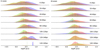 |
Fig. C.12 Radius ridge plots with zgal bins. Left (solid): VC sample. Right (dashed): MR sample. |
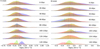 |
Fig. C.13 Velocity Dispersion ridge plots with zgal bins. Left (solid): VC sample. Right (dashed): MR sample. |
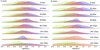 |
Fig. C.14 Aspect ratio ridge plots with zgal bins. Left (solid): VC sample. Right (dashed): MR sample. |
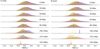 |
Fig. C.15 Virial parameter ridge plots with zgal bins. Left (solid): VC sample. Right (dashed): MR sample. |
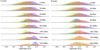 |
Fig. C.16 Length ridge plots with zgal bins. Left (solid): VC sample. Right (dashed): MR sample. |
References
- Arzoumanian, D., André, P., Didelon, P., et al. 2011, A&A, 529, L6 [NASA ADS] [CrossRef] [EDP Sciences] [Google Scholar]
- Arzoumanian, D., Russeil, D., Zavagno, A., et al. 2022, A&A, 660, A56 [NASA ADS] [CrossRef] [EDP Sciences] [Google Scholar]
- Ballesteros-Paredes, J., Hartmann, L. W., Vázquez-Semadeni, E., Heitsch, F., & Zamora-Avilés, M. A. 2011, MNRAS, 411, 65 [NASA ADS] [CrossRef] [Google Scholar]
- Ballesteros-Paredes, J., André, P., Hennebelle, P., et al. 2020, Space Sci. Rev., 216, 76 [Google Scholar]
- Barnes, P., Li, D., Telesco, C., et al. 2015, MNRAS, 453, 2622 [Google Scholar]
- Barnes, P. J., Hernandez, A. K., Muller, E., & Pitts, R. L. 2018, ApJ, 866, 19 [NASA ADS] [CrossRef] [Google Scholar]
- Beuther, H., Schneider, N., Simon, R., et al. 2022, A&A, 659, A77 [NASA ADS] [CrossRef] [EDP Sciences] [Google Scholar]
- Blitz, L., & Stark, A. A. 1986, ApJ, 300, L89 [CrossRef] [Google Scholar]
- Bresnahan, D., Ward-Thompson, D., Kirk, J. M., et al. 2018, A&A, 615, A125 [NASA ADS] [CrossRef] [EDP Sciences] [Google Scholar]
- Chapman, N. L., Goldsmith, P. F., Pineda, J. L., et al. 2011, ApJ, 741, 21 [NASA ADS] [CrossRef] [Google Scholar]
- Chen, C.-Y., Mundy, L. G., Ostriker, E. C., Storm, S., & Dhabal, A. 2020, MNRAS, 494, 3675 [Google Scholar]
- Colombo, D., Schinnerer, E., Hughes, A., et al. 2013, in American Astronomical Society Meeting Abstracts, 221, 349.16 [Google Scholar]
- Colombo, D., Rosolowsky, E., Ginsburg, A., Duarte-Cabral, A., & Hughes, A. 2015, MNRAS, 454, 2067 [NASA ADS] [CrossRef] [Google Scholar]
- Colombo, D., Rosolowsky, E., Duarte-Cabral, A., et al. 2019, MNRAS, 483, 4291 [NASA ADS] [CrossRef] [Google Scholar]
- Colombo, D., König, C., Urquhart, J. S., et al. 2021, A&A, 655, L2 [NASA ADS] [CrossRef] [EDP Sciences] [Google Scholar]
- Crutcher, R. M. 2012, ARA&A, 50, 29 [Google Scholar]
- Crutcher, R. M., Wandelt, B., Heiles, C., Falgarone, E., & Troland, T. H. 2010, ApJ, 725, 466 [NASA ADS] [CrossRef] [Google Scholar]
- Deharveng, L., Schuller, F., Anderson, L. D., et al. 2010, A&A, 523, A6 [NASA ADS] [CrossRef] [EDP Sciences] [Google Scholar]
- Dobbs, C. L., Krumholz, M. R., Ballesteros-Paredes, J., et al. 2014, in Protostars and Planets VI, eds. H. Beuther, R. S. Klessen, C. P. Dullemond, & T. Henning, 3 [Google Scholar]
- Duarte-Cabral, A., & Dobbs, C. L. 2016, MNRAS, 458, 3667 [NASA ADS] [CrossRef] [Google Scholar]
- Duarte-Cabral, A., Colombo, D., Urquhart, J. S., et al. 2021, MNRAS, 500, 3027 [Google Scholar]
- Elmegreen, B. G. & Lada, C. J. 1977, ApJ, 214, 725 [NASA ADS] [CrossRef] [Google Scholar]
- Field, G. B., Blackman, E. G., & Keto, E. R. 2011, MNRAS, 416, 710 [NASA ADS] [Google Scholar]
- Fukui, Y., Kawamura, A., Minamidani, T., et al. 2008, ApJS, 178, 56 [Google Scholar]
- Geen, S., Hennebelle, P., Tremblin, P., & Rosdahl, J. 2016, MNRAS, 463, 3129 [CrossRef] [Google Scholar]
- Güsten, R., Nyman, L. Å., Schilke, P., et al. 2006, A&A, 454, L13 [NASA ADS] [CrossRef] [EDP Sciences] [Google Scholar]
- Hacar, A., Tafalla, M., Kauffmann, J., & Kovács, A. 2013, A&A, 554, A55 [NASA ADS] [CrossRef] [EDP Sciences] [Google Scholar]
- Heyer, M., & Dame, T. M. 2015, ARA&A, 53, 583 [Google Scholar]
- Heyer, M., Krawczyk, C., Duval, J., & Jackson, J. M. 2009, ApJ, 699, 1092 [Google Scholar]
- Jaffa, S. E., Whitworth, A. P., Clarke, S. D., & Howard, A. D. P. 2018, MNRAS, 477, 1940 [NASA ADS] [CrossRef] [Google Scholar]
- Jayasinghe, T., Dixon, D., Povich, M. S., et al. 2019, MNRAS, 488, 1141 [NASA ADS] [CrossRef] [Google Scholar]
- Kainulainen, J., Stutz, A. M., Stanke, T., et al. 2017, A&A, 600, A141 [NASA ADS] [CrossRef] [EDP Sciences] [Google Scholar]
- Koda, J., Sawada, T., Hasegawa, T., & Scoville, N. Z. 2006, ApJ, 638, 191 [NASA ADS] [CrossRef] [Google Scholar]
- Larson, R. B. 1981, MNRAS, 194, 809 [Google Scholar]
- Li, G.-X., Urquhart, J. S., Leurini, S., et al. 2016, A&A, 591, A5 [NASA ADS] [CrossRef] [EDP Sciences] [Google Scholar]
- Liu, M., Li, D., Krco, M., et al. 2019, ApJ, 885, 124 [NASA ADS] [CrossRef] [Google Scholar]
- Luisi, M., Anderson, L. D., Schneider, N., et al. 2021, Sci. Adv., 7, eabe9511 [NASA ADS] [CrossRef] [Google Scholar]
- Mattern, M., Kauffmann, J., Csengeri, T., et al. 2018, A&A, 619, A166 [NASA ADS] [CrossRef] [EDP Sciences] [Google Scholar]
- Miville-Deschênes, M.-A., Murray, N., & Lee, E. J. 2017, ApJ, 834, 57 [Google Scholar]
- Neralwar, K. R., Colombo, D., Duarte-Cabral, A., et al. 2022, A&A, 663, A56 (Paper I) [NASA ADS] [CrossRef] [EDP Sciences] [Google Scholar]
- Olmi, L., Cunningham, M., Elia, D., & Jones, P. 2016, A&A, 594, A58 [NASA ADS] [CrossRef] [EDP Sciences] [Google Scholar]
- Polychroni, D., Schisano, E., Elia, D., et al. 2013, ApJ, 777, L33 [CrossRef] [Google Scholar]
- Rebolledo, D., Wong, T., Leroy, A., Koda, J., & Donovan Meyer, J. 2012, ApJ, 757, 155 [CrossRef] [Google Scholar]
- Rodgers, A. W., Campbell, C. T., & Whiteoak, J. B. 1960, MNRAS, 121, 103 [NASA ADS] [CrossRef] [Google Scholar]
- Roman-Duval, J., Jackson, J. M., Heyer, M., Rathborne, J., & Simon, R. 2010, ApJ, 723, 492 [NASA ADS] [CrossRef] [Google Scholar]
- Rosolowsky, E., & Leroy, A. 2006, Publ. ASP, 118, 590 [NASA ADS] [Google Scholar]
- Rosolowsky, E. W., Pineda, J. E., Kauffmann, J., & Goodman, A. A. 2008, ApJ, 679, 1338 [Google Scholar]
- Schneider, S., & Elmegreen, B. G. 1979, ApJS, 41, 87 [Google Scholar]
- Schneider, N., Simon, R., Guevara, C., et al. 2020, Publ. ASP, 132, 104301 [NASA ADS] [Google Scholar]
- Schuller, F., Csengeri, T., Urquhart, J. S., et al. 2017, A&A, 601, A124 [NASA ADS] [CrossRef] [EDP Sciences] [Google Scholar]
- Schuller, F., Urquhart, J. S., Csengeri, T., et al. 2021, MNRAS, 500, 3064 [Google Scholar]
- Snell, R. L., Loren, R. B., & Plambeck, R. L. 1980, ApJ, 239, L17 [NASA ADS] [CrossRef] [Google Scholar]
- Solomon, P. M., Rivolo, A. R., Barrett, J., & Yahil, A. 1987, ApJ, 319, 730 [Google Scholar]
- Sun, J., Leroy, A. K., Schruba, A., et al. 2018, ApJ, 860, 172 [NASA ADS] [CrossRef] [Google Scholar]
- Tiwari, M., Karim, R., Pound, M. W., et al. 2021, ApJ, 914, 117 [NASA ADS] [CrossRef] [Google Scholar]
- Urquhart, J. S., Figura, C., Cross, J. R., et al. 2021, MNRAS, 500, 3050 [Google Scholar]
- Vázquez-Semadeni, E., Palau, A., Ballesteros-Paredes, J., Gómez, G. C., & Zamora-Avilés, M. 2019, MNRAS, 490, 3061 [Google Scholar]
- Yuan, L., Yang, J., Du, F., et al. 2021, ApJS, 257, 51 [NASA ADS] [CrossRef] [Google Scholar]
- Zavagno, A., Deharveng, L., Comerón, F., et al. 2006, A&A, 446, 171 [NASA ADS] [CrossRef] [EDP Sciences] [Google Scholar]
- Zavagno, A., Pomarès, M., Deharveng, L., et al. 2007, A&A, 472, 835 [NASA ADS] [CrossRef] [EDP Sciences] [Google Scholar]
- Zhou, J., Zhou, D., Esimbek, J., et al. 2020, ApJ, 897, 74 [NASA ADS] [CrossRef] [Google Scholar]
- Zucker, C., Battersby, C., & Goodman, A. 2018, ApJ, 864, 153 [NASA ADS] [CrossRef] [Google Scholar]
- Zucker, C., Goodman, A., Alves, J., et al. 2021, ApJ, 919, 35 [NASA ADS] [CrossRef] [Google Scholar]
We remind the readers that the VC and MR samples used in this paper contain only the science sample clouds and therefore differ from the VC and MR samples presented in Paper I.
There are 25 elongated and 12 clumpy clouds with an aspect ratio <1.5 in the VC sample. These clouds are low resolution structures that might have been classified incorrectly or have unreliable medial axes measurements. We do not exclude these structures as they constitute only a very small percentage of the total sample and do not affect our analysis.
The distances are provided as R_gal and z_gal_kpc in the cloud catalogue of DC21.
The MR sample has ring-like clouds up to Rgal = 8 kpc only.
All Tables
Slopes and their standard deviations (SD) recovered from PCA on Larson’s scaling relation (συ ∝ Rslope) for the different cloud morphologies.
P-values for the two-sample KS test conducted on the VC and MR samples for each property and morphology.
P-values for the two-sample KS test conducted on the different morphologies for each cloud property (VC sample).
All Figures
|
Fig. 1 Examples of different cloud morphologies. The images are integrated intensity (moment 0) maps of the 13CO (2−1) transition. The numbers in the right bottom corner of the images represent the J1 and the J2 moments (J plots algorithm), respectively. The colour bars represent the 13CO integrated intensity in K kms–1. The white contours represent the cloud edge. The white circles at the bottom left of the figures represent the telescope beam size. |
| In the text | |
|
Fig. 2 Distribution of radius (top) and velocity dispersion (bottom) for the VC (blue) and MR (orange) samples. The violin plots present the density of the data at different values, which is smoothed through kernel density estimation. The horizontal lines at the ends and middle of the plots represent the extreme and the median values of the distributions, respectively. |
| In the text | |
|
Fig. 3 Distribution of length (top) and aspect ratio (bottom). The symbols and conventions follow Fig. 2. |
| In the text | |
|
Fig. 4 Distribution of mass (top) and surface density (bottom). The symbols and conventions follow Fig. 2. |
| In the text | |
|
Fig. 5 Distribution of virial parameter for the VC and MR samples. The symbols and conventions follow Fig. 2. |
| In the text | |
|
Fig. 6 Histogram (normalised) for distribution of clouds with respect to Galactocentric radius (top) Galactic height (zgal) (middle), and heliocentric distance (bottom). The histograms represent the ratio of clouds in each bin to the total number of clouds in all the bins. The bin width is 1 kpc for the heliocentric distance and Galactocentric radius plots, and 1 pc for the zgal histogram. Blue represents the VC sample and orange represents the MR sample. The cloud morphologies from top to bottom represent ring-like clouds (Ring), elongated clouds (Elon), concentrated clouds (Cone), and clumpy clouds (Clumpy). |
| In the text | |
|
Fig. 7 Size-linewidth relation (συ versus R) using the MR sample. The dashed line represents Larson’s first relation (Larson 1981; Solomon et al. 1987). The different colours represent four cloud classes (Sect. 3); ring-like clouds are represented in blue, elongated clouds in red, concentrated clouds in green, and clumpy clouds in magenta. The contours include 68% of the data (1–sigma level) and the small circles represent centroids (means) of the distributions. The expected slope for the relation is 0.5 (dashed black line) (Larson 1981). |
| In the text | |
|
Fig. 8 Scaling relation between |
| In the text | |
|
Fig. B.1 Mass ridge plot for the VC sample with Rd bins. |
| In the text | |
|
Fig. B.2 Mass ridge plot for the MR sample with Rd bins. |
| In the text | |
|
Fig. B.3 Surface density ridge plots with Rd bins. Left (solid): VC sample. Right (dashed): MR sample. |
| In the text | |
|
Fig. B.4 Radius ridge plots with Rd bins. Left (solid): VC sample. Right (dashed): MR sample. |
| In the text | |
|
Fig. B.5 Velocity dispersion ridge plots with Rd bins. Left (solid): VC sample. Right (dashed): MR sample. |
| In the text | |
|
Fig. B.6 Aspect ratio ridge plots with Rd bins. Left (solid): VC sample. Right (dashed): MR sample. |
| In the text | |
|
Fig. B.7 Virial parameter ridge plots with Rd bins. Left (solid): VC sample. Right (dashed): MR sample. |
| In the text | |
|
Fig. B.8 Length ridge plots with Rd bins. Left (solid): VC sample. Right (dashed): MR sample. |
| In the text | |
|
Fig. C.1 Mass ridge plot for the VC sample with Rgal bins. The vertical dashed lines represent the medians of the distributions. |
| In the text | |
|
Fig. C.2 Mass ridge plot for the MR sample with Rgal bins. The vertical dashed lines represent the medians of the distributions. |
| In the text | |
|
Fig. C.3 Surface density ridge plots with Rgal bins. Left (solid): VC sample. Right (dashed): MR sample. |
| In the text | |
|
Fig. C.4 Radius ridge plots with Rgal bins. Left (solid): VC sample. Right (dashed): MR sample. |
| In the text | |
|
Fig. C.5 Velocity Dispersion ridge plots with Rgal bins. Left (solid): VC sample. Right (dashed): MR sample. |
| In the text | |
|
Fig. C.6 Aspect ratio ridge plots with Rgal bins. Left (solid): VC sample. Right (dashed): MR sample. |
| In the text | |
|
Fig. C.7 Virial Parameter ridge plots with Rgal bins. Left (solid): VC sample. Right (dashed): MR sample. |
| In the text | |
|
Fig. C.8 Length ridge plots with Rgal bins. Left (solid): VC sample. Right (dashed): MR sample. |
| In the text | |
|
Fig. C.9 Mass ridge plot for the VC sample with zgal bins. |
| In the text | |
|
Fig. C.10 Mass ridge plot for the MR sample with zgal bins. |
| In the text | |
|
Fig. C.11 Surface density ridge plots with zgal bins. Left (solid): VC sample. Right (dashed): MR sample. |
| In the text | |
|
Fig. C.12 Radius ridge plots with zgal bins. Left (solid): VC sample. Right (dashed): MR sample. |
| In the text | |
|
Fig. C.13 Velocity Dispersion ridge plots with zgal bins. Left (solid): VC sample. Right (dashed): MR sample. |
| In the text | |
|
Fig. C.14 Aspect ratio ridge plots with zgal bins. Left (solid): VC sample. Right (dashed): MR sample. |
| In the text | |
|
Fig. C.15 Virial parameter ridge plots with zgal bins. Left (solid): VC sample. Right (dashed): MR sample. |
| In the text | |
|
Fig. C.16 Length ridge plots with zgal bins. Left (solid): VC sample. Right (dashed): MR sample. |
| In the text | |
Current usage metrics show cumulative count of Article Views (full-text article views including HTML views, PDF and ePub downloads, according to the available data) and Abstracts Views on Vision4Press platform.
Data correspond to usage on the plateform after 2015. The current usage metrics is available 48-96 hours after online publication and is updated daily on week days.
Initial download of the metrics may take a while.