| Issue |
A&A
Volume 663, July 2022
|
|
|---|---|---|
| Article Number | A56 | |
| Number of page(s) | 39 | |
| Section | Interstellar and circumstellar matter | |
| DOI | https://doi.org/10.1051/0004-6361/202142428 | |
| Published online | 13 July 2022 | |
The SEDIGISM survey: Molecular cloud morphology
I. Classification and star formation★
1
Max-Planck-Institut für Radioastronomie,
Auf dem Hügel 69,
53121
Bonn, Germany
e-mail: This email address is being protected from spambots. You need JavaScript enabled to view it.
2
School of Physics & Astronomy, Cardiff University,
Queen’s building, The parade,
Cardiff
CF24 3AA, UK
3
Centre for Astrophysics and Planetary Science, University of Kent,
Canterbury
CT2 7NH, UK
4
Laboratoire d’Astrophysique (AIM), CEA, CNRS, Université Paris-Saclay, Université Paris Diderot,
Sorbonne Paris Cité,
91191
Gif-sur-Yvette, France
5
Space Science Institute,
4765 Walnut St Suite B,
Boulder, CO
80301, USA
6
School of Science and Technology, University of New England,
Armidale NSW
2351, Australia
7
I. Physikalisches Institut, Universität zu Köln,
Zülpicher Strasse 77,
50937
Cologne, Germany
8
Max-Planck-Institut für Astronomie,
Königstuhl 17,
69117
Heidelberg, Germany
9
Astrophysics Research Institute, Liverpool John Moores University,
IC2, Liverpool Science Park, 146 Brownlow Hill,
Liverpool
L3 5RF, UK
10
Laboratoire d’astrophysique de Bordeaux, CNRS, Univ. Bordeaux,
B18N, allée Geoffroy Saint-Hilaire,
33615
Pessac, France
11
School of Physics and Astronomy, University of Exeter,
Stocker Road,
Exeter
EX4 4QL, UK
12
Leibniz-Institut für Astrophysik Potsdam (AIP),
An der Sternwarte 16,
14482
Potsdam, Germany
13
INAF – Osservatorio Astronomico di Cagliari,
Via della Scienza 5,
09047
Selargius (CA), Italy
14
The American University of Paris,
2bis, Passage Landrieu
75007
Paris, France
Received:
13
October
2021
Accepted:
4
March
2022
Abstract
We present one of the very first extensive classifications of a large sample of molecular clouds based on their morphology. This is achieved using a recently published catalogue of 10 663 clouds obtained from the first data release of the Structure, Excitation and Dynamics of the Inner Galactic InterStellar Medium (SEDIGISM) survey. The clouds are classified into four different morphologies via visual inspection and using an automated algorithm – J plots. The visual inspection also serves as a test for the J plots algorithm as this is the first time it has been used on molecular gas. Generally, it has been found that the structure of molecular clouds is highly filamentary, and our observations indeed verify that most of our molecular clouds are elongated structures. Based on our visual classification of the 10 663 SEDIGISM clouds, 15% are ring-like, 57% are elongated, 15% are concentrated, and 10% are clumpy clouds. The remaining clouds do not belong to any of these morphology classes and are termed unclassified. We compare the SEDIGISM molecular clouds with structures identified through other surveys: the elongated structures from the APEX Telescope Large Area Survey of the Galaxy (ATLASGAL) and the bubbles from Milky Way Project (MWP). We find that many of the ATLASGAL and MWP structures are velocity coherent. Elongated ATLASGAL structures overlap with ≈21% of the elongated SEDIGISM structures (elongated and clumpy clouds), and MWP bubbles overlap with ≈25% of the ring-like SEDIGISM clouds. We also analyse the star formation associated with different cloud morphologies using two different techniques. The first technique examines star formation efficiency and the dense gas fraction based on SEDIGISM cloud and ATLASGAL clump data. The second technique uses the highmass star formation threshold for molecular clouds. The results indicate that clouds with ring-like and clumpy morphologies show a higher degree of star formation.
Key words: ISM: clouds / local insterstellar matter / ISM: bubbles / stars: formation / submillimeter: ISM
Tables A.1–A.4 are only available at the CDS via anonymous ftp to cdsarc.u-strasbg.fr (130.79.128.5) or via http://cdsarc.u-strasbg.fr/viz-bin/cat/J/A+A/663/A56
Member of the International Max Planck Research School (IMPRS) for Astronomy and Astrophysics at the universities of Bonn and Cologne.
© K. R. Neralwar et al. 2022
 Open Access article, published by EDP Sciences, under the terms of the Creative Commons Attribution License (https://creativecommons.org/licenses/by/4.0), which permits unrestricted use, distribution, and reproduction in any medium, provided the original work is properly cited.
Open Access funding provided by Max Planck Society.
1 Introduction
Molecular clouds are often approximated as self-gravitating spheres (Rosolowsky & Leroy 2006; Benedettini et al. 2021), especially for the calculation of the cloud size (radius). Nevertheless, modern surveys have shown that molecular gas is organised in a more complex fashion. In particular, molecular gas appears permeated by filamentary structures (André et al. 2010; Jackson et al. 2010; Molinari et al. 2010; Li et al. 2016; Duarte-Cabral & Dobbs 2017; Zucker et al. 2018; Arzoumanian et al. 2019; Suri et al. 2019; Zhang et al. 2019; Abe et al. 2021; Priestley & Whitworth 2022; Yuan et al. 2021; Colombo et al. 2021). Thus, an analysis of the connection between molecular clouds and structures such as filaments and bubbles can improve our understanding of the various phenomena in the interstellar medium (ISM), for example star formation.
The presence of filaments in molecular clouds as sites of formation of pre-stellar and proto-stellar cores has been a popular topic of discussion in star formation research (André et al. 2014; Li et al. 2016; Arzoumanian et al. 2017; Mattern et al. 2018a; Zhang et al. 2019; Bonne et al. 2020b). The existence of filaments in star-forming regions has been evident through decades of observations (Schneider & Elmegreen 1979; Ragan et al. 2014; Marsh et al. 2016; Suri et al. 2019; Schisano et al. 2020), accompanied by numerical simulations (Klessen & Burkert 2000; Padoan et al. 2001; Heitsch et al. 2008; Hennebelle et al. 2008; Nakamura & Li 2008; Vázquez-Semadeni et al. 2011). The sizes of filaments range from sub-parsec scales (mostly seen in nearby regions; André et al. 2010; Arzoumanian et al. 2019) to hundreds of parsecs (Schisano et al. 2014, 2020; Wang et al. 2015, 2020; Mattern et al. 2018a; Lin et al. 2020). These large-scale filaments are often associated with galactic spiral arms (Wang et al. 2015) and are seen as chains of smaller filaments; for example, the active star formation sites in the filaments are visible in infrared observations whereas the quiescent parts are infrared dark (infrared dark clouds; Peretto & Fuller 2010).
Herschel images (Hi-GAL survey; Molinari et al. 2010; Zavagno et al. 2010; Schisano et al. 2020) have revolutionised the study of filaments in the Milky Way, exhibiting their abundance in the Galaxy (within molecular clouds) and introducing constraints on their formation and evolution. The formation of filaments in galaxies is often attributed to the shock waves permeating the ISM (Arzoumanian et al. 2018, and references therein). Cloud collisions also result in filament formation, and these filaments fragment into smaller components due to turbulence and gravitational instabilities (Balfour et al. 2015; Bonne et al. 2020a; Liow & Dobbs 2020; Dobbs & Wurster 2021; Clarke et al. 2020; Fukui et al. 2021). These dense (supercritical) filaments often fragment into star-forming cores, thus leading to star formation (André et al. 2010; Könyves et al. 2015; Arzoumanian 2017).
The molecular gas in clouds often gets dispersed and expelled due to stellar radiation and winds, resulting in the formation of ring-like objects called bubbles or shells. Infrared bubbles are often associated with triggered star formation and usually encompass an HII region (Deharveng et al. 2010; Schneider et al. 2020). Whether the ring-like appearance of bubbles is a consequence of its 3D structure or a projection effect is debatable (Churchwell et al. 2006; Beaumont & Williams 2010; Pabst et al. 2020). The expansion of HII regions drives a shock wave into the molecular clouds, sweeping up the gas (Francis et al. 1998; Bialy et al. 2021). It further causes the entrapment of neutral material between the ionised and shock fronts, giving rise to dense rings of molecular gas. Stellar winds from massive stars create X-ray dominated regions, aiding the formation of these bubbles and the cold material in the shell, which may become gravitationally unstable and host star formation (Zavagno et al. 2006; Deharveng et al. 2009). Low-mass stars can readily be formed due to small-scale instabilities such as the Jeans instability, whereas large-scale gravitational instabilities can eventually lead to high-mass star formation (HMSF; Habing et al. 1972; Elmegreen & Lada 1977; Krumholz 2006). The mass of a star is also influenced by its environment (Rosen et al. 2020).
Many infrared detections of bubbles have come from images by the Infrared Space Observatory and the Midcourse Space Experiment, which culminated in high-resolution surveys of the Milky Way such as the Galactic Legacy Infrared Mid-Plane Survey Extraordinaire (GLIMPSE; Churchwell et al. 2006) and the Herschel infrared Galactic Plane Survey (Hi-GAL; Molinari et al. 2010; Carey 2016). They have been used to understand the mechanisms behind bubble formation while associating them with objects such as supernovae, planetary nebulae, open clusters, Wolf-Rayet stars, and OB stars. Churchwell et al. (2007) postulate that most of the bubbles are produced by stars with strong winds, O stars and B stars. OB stars often have HII regions associated with them, whereas late-B stars produce small bubbles by exciting polycyclic aromatic hydrocarbon (PAH) bands without forming HII regions. Simulations that include ionisation find that bubbles or shells readily form within molecular clouds (e.g. Dale et al. 2005; Geen et al. 2015; Ali & Harries 2019; Li et al. 2019; Bending et al. 2020; Fukushima & Yajima 2021; Grudic et al. 2021). These simulations typically start with spherical molecular clouds; for more massive clouds or at earlier times, the feedback may not be sufficient to break out of the clouds, and a complete ring that contains an HII region occurs. On the other hand, for lower-mass clouds, the feedback is often sufficient to break out of and, in some cases, disperse the cloud. Generally, numerical simulations find that photoionisation appears to dominate compared to stellar winds (Dale et al. 2014; Haid et al. 2018, 2019; Grudic et al. 2021; Geen et al. 2021; Ali et al. 2022).
As particular gas morphologies appear to be connected to a specific set of physical phenomena, a study of the molecular cloud morphology can aid the study of star formation and other complex processes, such as stellar feedback, that drive turbulence in the ISM, result in the disruption of molecular clouds, and lead to the formation of structures (e.g. bubbles). Recently, identifications of molecular clouds from large-scale surveys have been carried out efficiently using automated methods, for example dendrogram analysis (Rosolowsky et al. 2008), scimes (Colombo et al. 2015), and CPROPS (Rosolowsky & Leroy 2006; Rosolowsky et al. 2021). A robust large-scale cloud catalogue is presented by Duarte-Cabral et al. (2021) (hereafter DC21), who identified molecular clouds from the Structure, Excitation and Dynamics of the Inner Galactic InterStellar Medium (SEDIGISM) survey using the scimes algorithm. We employ the J plot algorithm (Jaffa et al. 2018) and a visual classification technique to classify the SEDIGISM molecular clouds into various morphologies, and this forms the core of this work. We thus try to understand whether different cloud morphologies host different types of star formation.
In this paper we present the morphological classification for the 10663 clouds identified in the SEDIGISM survey by DC21. In Sect. 2 we describe the datasets from three surveys – SEDIGISM, the APEX Telescope Large Area Survey of the Galaxy (ATLASGAL), and the Milky Way Project (MWP) – used throughout the paper. Section 3 describes the two methods used to classify the clouds into different morphologies (i.e. J plots and by-eye classification). In Sect. 4 we discuss the pros and cons of the J plot classification by comparing it with visual classification. Our results are presented and discussed in Sect. 5. In Sect. 5.1 we compare the SEDIGISM clouds to the filamentary structures from the ATLASGAL survey and dust bubbles from MWP. We thus reveal the SEDIGISM clouds that overlap with these structures and find possible coherent ATLASGAL and MWP structures. In Sect. 5.2 we use two different methods to study the star formation associated with different morphologies. Finally, we summarise our findings in Sect. 6.
2 Data
We use catalogues from three surveys in this paper – molecular clouds from SEDIGISM, elongated (filamentary) structures from ATLASGAL, and bubbles derived from the infrared data in the MWP.
2.1 Sedigism
The SEDIGISM survey covers a region of 84 deg2 between −60° ≤ l ≤ +18° and |b| ≤ 0.5° (b varies in some regions) using various molecular tracers; in particular, the J = 2−1 transitions of 13CO and C18O. These observations were conducted using the 12m Atacama Pathfinder Experiment (APEX; Güsten et al. 2006) during 2013–2017. A complete description of the SEDIGISM1 survey is presented in Schuller et al. (2017, 2021).
The survey data (complete contiguous dataset) is presented in the form of 77 datacubes of approximately 2° × 1° with velocities from −200 to 200 km s−1 and pixel size of 9.5″, and these are centred on all integer Galactic longitudes. The DR1 includes 13CO observations, with a full width at half maximum beam size of 28″ and typical 1σ sensitivity of 0.8−1.0 K per 0.25 km s−1. A catalogue of 10 663 molecular clouds (full sample) has been identified from the contiguous dataset of SEDIGISM survey DR1 (13CO) and is presented in DC21. The molecular clouds have been extracted using the Spectral Clustering for Interstellar Molecular Emission Segmentation scimes algorithm (v.0.3.2) (Colombo et al. 2015, 2019). These clouds from the catalogue are hereafter referred to as SEDIGISM clouds. Furthermore, we use SEDIGISM clouds to define two new cloud sub-samples for our morphological analysis (see Sect. 4.1).
2.2 Atlasgal
ATLASGAL (Schuller et al. 2009) is an unbiased survey of the inner Galaxy aimed at studying sites of star formation. It observes the dust continuum emission at 870 μm, in the region 280° < l < 60° and |b| < 1.5° (b varies between −2° and 1° for l < 300°). The observations were carried out using the Large Apex BOlometer CAmera instrument (Siringo et al. 2009) at a typical noise level of 50–70 mJy beam−1 and a beam size of 19.2″. The survey has identified more than 10000 dense clumps (Contreras et al. 2013; Csengeri et al. 2014; Urquhart et al. 2014, 2018) of masses ~500 M⊙ and sizes ~0.5 pc. Urquhart et al. (2021) has compared these clumps to the SEDIGISM clouds and obtained star formation efficiencies (SFEs) and dense gas fractions (DGFs) for these clouds. The SFEs and DGFs were obtained using cloud masses, integrated clump masses, and their bolometric luminosities. We explore the differences in SFE and DGF for various cloud morphologies in Sect. 5.2.1.
Li et al. (2016) identified spatially coherent filamentary structures from ATLASGAL data using the Discrete Persistent Structures Extractor (DisPerSE) algorithm. DisPerSE is a source extractor algorithm based on discrete Morse theory that identifies topological features from 2D and 3D datasets, thus extracting the necessary skeletons. A catalogue of 1812 structures was obtained using this method, and these were subsequently visually inspected and classified into five types: marginally resolved clumps, resolved elongated structures, filaments, networks of filaments and complexes. We use the three elongated-type structures (i.e. filaments, networks of filaments and resolved elongated structures) and compare them with SEDIGISM clouds (Sect. 5.1). Hereafter we refer to these three structures collectively as ATLASGAL elongated structures (AG-Els) whereas the filaments are individually refereed to as ATLASGAL filaments (AG-Fils).
2.3 Mwp
The MWP (Simpson et al. 2012; Jayasinghe et al. 2019) is a citizen science project aimed at identification of bubbles and bow shocks from the infrared images obtained using Spitzer Space Telescope Galactic plane surveys. It was launched in 2010 and provided the users with 4.5 and 8 μm images from GLIMPSE (Benjamin et al. 2003; Churchwell et al. 2009) and 24 μm images from the MIPS Galactic Plane Survey survey (MIPSGAL Carey et al. 2009). The DR1 (Simpson et al. 2012) was released in 2012 and has produced a catalogue of over 5000 bubbles.
The second data release of MWP culminates the visual analysis of 31000+ citizen scientists during 2012–2017. It has identified Galactic structures by inspection of images from GLIMPSE, MIPSGAL, Spitzer Mapping of the Outer Galaxy (SMOG; Carey et al. 2008) and Cygnus-X (Hora et al. 2009) surveys. The project observes 0° < l < 65°, 295° < l < 360° and |b| < 1° and a few additional regions. The bubbles were identified using an ellipse drawing tool to mark the location and shape of bubbles. The identification quality was tested by comparing the bubbles to observations carried out by trained experts and using machine-learning algorithms. We use the 2600 bubbles (Jayasinghe et al. 2019) identified from the DR2 to compare with the SEDIGISM clouds in Sect. 5.1.
3 Methodology
We use the SEDIGISM data cubes with 3D masks (produced by DC21) to generate integrated intensity maps (Figs. 1–5) of individual clouds. These are 2D (integrated intensity masked) images obtained by integrating the intensity in a 3D cube along the velocity axis. These images are used to classify the clouds into different morphologies using two methods. The first method – J plot – is an automated algorithm whereas the second method – by-eye classification – implies classification of clouds carried out visually by the lead author. The cloud classifications are provided as a catalogue, which is further described in Appendix A.
3.1 J plots
J plots (Jaffa et al. 2018) is a method to classify and quantify a pixelated structure into different morphologies using its moment of inertia (i.e. the degree of elongation and the degree of concentration). The classification procedure involves the calculation of the principal moments of inertia (I1 and I2) for each cloud, using the surface density and area covered (in pixels). The I1 and I2 are the principal moments of inertia along the two principal axes of the structure, such that the first principal axis is associated with the smaller principal moment, thus I1 ≤ I2. These moments are then compared with the principal moment for a uniform surface density disk  of same area (A) and mass (M) and hence converted into ‘J’ moments J1 and J2 as
 (1)
(1)
J plots makes use of the connection between moment of inertia and mass concentration. For example, an increase in the concentration of mass towards the centre results in the decrease of the moment of inertia of the structure. This is used to identify centrally concentrated disks. The original algorithm (described in Jaffa et al. 2018) uses the dendrograms to segment images and generate hierarchical structures directly from the raw data. However, in this work, the input to the algorithm are the 2D cloud images (e.g. Fig. 1) generated via scimes, and its only purpose is morphological classification. The structures are classified into three types based on their J moments: (i) centrally concentrated disks (cores): J1 > 0, J2 > 0; (ii) elongated ellipses (filaments): J1 > 0, J2 < 0; and (iii) rings (limb-brightened bubbles): J1 < 0, J2 < 0.
The original implementation of J plots was based on dust continuum surface-density maps (Jaffa et al. 2018). However, we apply the J plots algorithm on CO integrated-intensity images, and it leads to a slight change in the terminology. Due to the non-trivial derivation of distances in the Milky Way, it is difficult to directly obtain the surface density and mass of the structures from the integrated-intensity images and thus we use the pixel weights and total structure weights in their place, respectively. However, these differences do not pose any changes in the overall classification scheme. The morphological classes resulting from the J-plot classification are hereafter collectively referred to as J-structures, and individually as J-core, J-filament and J-bubble (e.g. Fig. 6).
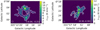 |
Fig. 1 Examples of two ring-like clouds as per the visual classification method. Left: J-bubble, cloud ID 238. Right: J-filament, cloud ID 3148. The cloud identification numbers (cloud IDs) can be used to identify the cloud structure from the main catalogue (Table A.1). The images are integrated intensity (moment 0) maps of the 13CO (2–1) transition. The numbers in the bottom-right corner of the images represent the J1 and the J2 moments, respectively. The colour bar represents the 13CO integrated intensity in K km s−1. The white contour represents the cloud edge. The white circle at the bottom left of the figure represents the telescope beam size. The black ellipse on the second image represents an artistic impression of the visualised ring. |
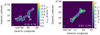 |
Fig. 2 Examples of two elongated clouds as per the visual classification method. Left: J-filament, cloud ID 1726. Right: J-filament, cloud ID 130. The conventions follow Fig. 1. |
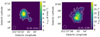 |
Fig. 3 Examples of two concentrated clouds as per the visual classification method. Left: J-filament, cloud ID 3133. Right: J-core, cloud ID 6567. The conventions follow Fig. 1. |
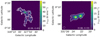 |
Fig. 4 Examples of two clumpy clouds as per the visual classification method. Left: J-filament, cloud ID 2500. Right: J-filament, cloud ID 3010. The conventions follow Fig. 1. |
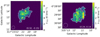 |
Fig. 5 Examples of two unclassified clouds. Left: J-filament, cloud ID 1445. Right: J-filament, cloud ID 3976. The conventions follow Fig. 1. |
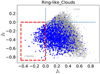 |
Fig. 6 J plot for the visual class ring-like clouds. The blue dots represent the ring-like clouds, and the grey dots represent all the clouds in VC sample. The blue dots lying inside the red dashed rectangle represent the MR sample. |
3.2 By-eye classification
We performed a visual inspection of the integrated intensity maps of clouds (e.g. Fig. 1) and classified them into four different morphological classes. Three of the classes – ring-like, elongated and concentrated cloud – are inspired from J plots. We defined the fourth class of clouds, referred to as clumpy clouds, by combining smaller sub-classes2 on the basis of the two-sample Kolmogorov-Smirnov (KS) test and the two-sided Mann–Whitney U (MWU) test. The KS and MWU tests are non-parametric tests. The KS test has a null hypothesis that the two samples are drawn from the same distribution. The MWU test has a null hypothesis that neither distribution has statistical dominance over the other. We discuss the two test in details in Appendix C. The p-values presented in this work are obtained using the two-sample KS test and the two-sided MWU test. The visual classification provides a method to independently verify the J plot classification. The morphologies are as follows: (i) Ring-like clouds are clouds that resemble a ring or a bubble (Fig. 1) and are comparable to J-bubbles. (ii) Elongated clouds are clouds that are elongated in nature (Fig. 2) and maintain a visibly uniform structure. They are comparable to J filaments. (iii) Concentrated clouds are clouds that have most of their integrated intensity densely packed into a compact region (Fig. 3). These clouds have a spherical geometry and are comparable to J cores. (iv) Finally, clumpy clouds are elongated clouds with the presence of one or more smaller (visible) clumps (denser regions) (Fig. 4). They are comparable to J filaments.
There are 298 clouds that do not fit the description of any of the above morphologies (Fig. 5). They are typically diffuse in nature and close to the resolution element of the survey. These clouds are termed as unclassified, and we exclude them in our analysis (refer Sect. 4.1).
3.3 Limitations of the classification methods
J plots is aimed at producing an automated classification of filaments, cores and bubbles by analysing their surface-density emission. The algorithm is currently limited to detection (using dendrograms) and analysis of 2D structures from images. Jaffa et al. (2018) has applied J plots on the region around RCW 120 using data from the Hi-GAL survey and successfully identified the previously known bubble and other ring-like structures. It also confirmed that in the third quadrant of the J plots (J1 < 0 & J2 < 0), the distance from the origin reflects the thickness of the ring (bubble). Similarly, it has also identified and quantified filaments from the smoothed-particle hydrodynamics simulation of Clarke et al. (2017).
We used the velocity coherent SEDIGISM clouds identified in 3D position-position-velocity (PPV) space and provided them to J plots after integrating along the velocity axis. Therefore, the morphological analysis was done in 2D space. J plot assumes strict limits of principal (and J) moments for all structures; for example, in the case of bubbles, both the J moments are negative. This may lead to an incorrect classification of some structures. For example, the interaction of an OB star with the ambient ISM can lead to deformities in the circular shape of a bubble (Jayasinghe et al. 2019). It could lead to one J moment being positive for the structure, resulting in its identification as a filament instead of a bubble. Hence, elliptic bubbles might be incorrectly classified by J plots. We also see in Table 1 that J plot classifies 87% of the clouds as filaments while visual classification identifies only 67% of the clouds as elongated structures (elongated & clumpy clouds). However, our visual (by-eye) classification is not completely unambiguous. For example, some clouds display both clumpy structure and partial rings. We also see clouds with small curved branches along otherwise long filaments. To minimise the uncertainties in cloud classification, we present the morphologically reliable (MR) sample in Sect. 4.1.
As our analysis is performed in 2D space, we only see a projected image of the molecular clouds and this can lead to an incorrect morphological classification. For example, a filament lying completely in the line of sight of the telescope can appear to be concentrated in a small region, thus leading to its classification as a core. However, due to the large size of our sample, the projection effects are unlikely to affect the general results.
We also tested if the morphological classification is affected by the noise in the data. The SEDIGISM cloud catalogue (DC21) contains the S/N for each cloud. We chose the 1000 clouds with the |J1| values closest to zero, and chose the 100 noisiest clouds (lowest S/N) from them. Similarly, we chose the 100 noisiest clouds closest to |J2| = 0. These 200 clouds are introduced with random noise (~ average noise in the SEDIGISM data cube to which the cloud belongs) and their morphologies are identified with J plots. We observe that only three clouds3 show a change in the morphology (from core to filament), which indicates that the J plots classification is mostly robust against the changes in noise.
Quantitative description of cloud groups.
4 Morphological classification
4.1 Visually classified (VC) and morphologically reliable (MR) samples
We use the SEDIGISM cloud sample to create two samples to study the cloud morphology. These are the VC and MR samples. The VC sample is obtained from the by-eye classification of full sample by discarding the unclassified clouds (Sect. 3). The MR sample is a sub-sample of the VC sample, containing only the clouds for which the J plots and by-eye classification morphologies are in agreement (i.e. the clouds’ morphology is consistent for the two methods; see Figs. 6–9). Therefore, a cloud belongs to the MR sample only if it satisfies one of the four following conditions: (i) it is a ring-like cloud classified as a bubble by J plot; (ii) it is an elongated cloud classified as a filament by J plot; (iii) it is a concentrated cloud classified as a core by J plot; or (iv) it is a clumpy cloud classified as a core or filament by J plot.
The clumpy clouds contain only the elongated clouds with clumps in them. We include the J cores as they might have elongated structure but recognised as a core due to high central density (Fig. 9). In Table 1, we list the total number of clouds assigned to each group. In brief, the MR sample contains clouds with the most reliable morphological classification and should be preferred. However, it excludes a large number of SEDIGISM clouds and has a low sample size, especially for ring-like clouds. A larger sample is the VC sample but it might contain subjective biases. In the parallel paper (Neralwar et al. in prep), we confirm that the distance distributions of both the samples follow each other closely. We also study the SEDIGISM cloud properties using the two samples and their results are in agreement.
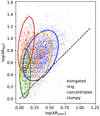 |
Fig. 10 Comparison between aspect ratios obtained using the moment technique (ARmom) and the medial axis technique (ARma) for different cloud morphologies. The ellipses encompass approximately 95% of the respective data points (two-sigma level). The dashed black line represents the 1:1 relation. |
4.2 Aspect ratio: Moments technique versus medial axis
We used our most reliable sample – the MR sample – to check whether the aspect ratios obtained using two different methods show some trends with respect to different morphologies (Fig. 10) or whether both methods provide the same information regarding the aspect ratio of the structures. The first method to obtain the aspect ratio is the moment technique (described in Rosolowsky & Leroy 2006). It uses principal component analysis (PCA) to determine the orientation of the major axis of a cloud. The geometric mean of the second spatial moments gives the rms size of the cloud along the two orthogonal axes. The ratio of this intensity weighted major and minor axes gives the aspect ratio – ARmom. The ARmom values for each cloud have been automatically calculated while building the catalogue for the dendrograms of emission and are provided in the SEDIGISM cloud catalogue (DC2l).
The second method to obtain an estimate of the aspect ratio is using a geometrical medial axis (a quantity also computed by DC2l, and provided in the cloud catalogue). Such a medial axis is the longest-running spine passing centrally through the entire length of a 2D projected cloud mask. The cloud length is the medial axis length, whereas the cloud (medial axis) width is twice the average distance from this central spine to the cloud edge. The ratio of the medial axis length to medial axis width gives the aspect ratio – ARMA. The medial axis length is free of the assumption that clouds have any particular geometry and hence provides an alternative estimate of the cloud ‘shape’.
We compare the two aspect ratios for the MR sample in Fig. 10, where a rough distinction between the different morphologies is seen. The two approaches give different aspect ratios for the same cloud depending on the cloud’s morphology and potentially also the internal structure (as the moment method takes into account the pixel intensity to calculate the two semi-axis lengths). We might expect the aspect ratios to diverge for complex structures, while to give more comparable measurements for simpler shaped clouds, such as the concentrated objects. For instance, the majority of ring-like clouds do not form a complete ring. The moment technique (PCA) intrinsically perceives these clouds as elliptical structures whereas medial axis runs along their shell. This leads to ARma being a ratio of the perimeter and thickness of cloud shell whereas ARmom traces a more spherical geometry, relating more to the size of the bubble that created the ring. Hence, we expect ring-like clouds to have a typically low ARmom but a high ARMA. This effect might be not so pronounced in the case of other morphologies, leading to concentrated clouds having both aspect ratios with low values, while elongated and clumpy clouds are expected to have high ARmom and ARMA. Nevertheless, in almost every case, ARMA appears to be larger than ARmom. We conclude that aspect ratio measuring methods can give widely different results depending on the cloud morphology and the complexity, and they need to be used with care.
5 Results and discussion
5.1 Cloud counterparts from other surveys
In this section we compare the positions of SEDIGISM clouds and the structures from ATLASGAL and MWP. It helps us to understand how the low-density molecular gas follows the dense structures observed through ATLASGAL. The comparison may shed light on the connection between AG-El and elongated clouds. MWP traces PAH regions, HII regions and warm dust, which have a higher excitation temperature than the 13CO emission (Mazumdar et al. 2021). These regions (bubbles) are often a consequence of the stellar feedback from massive stars. We use these bubbles to study whether the molecular gas surrounding these regions is detected as our ring-like clouds. ATLASGAL and MWP are continuum surveys and the corresponding structures lack velocity information. Therefore, we compare the positions of clouds and (ATLASGAL and MWP) structures only in 2D position-position (p-p) space. The positions of pixels for each AG-El are provided in Li et al. (2016). The MWP bubble catalogue (Jayasinghe et al. 2019) contains cen-troids for the ellipses (bubbles) and their major and minor axes. These parameters give us the position of the bubble but they do not provide us any information about the completeness of the ring. We use these parameters and pixel positions to compare the position of these structures with SEDIGISM clouds.
The lack of velocity information for continuum structures can be addressed for the structures that uniquely match with a single SEDIGISM cloud. SEDIGISM clouds are obtained using the scime s algorithm on the 3D PPV data cubes and therefore are coherent structures. Hence, the ATLASGAL and MWP structures that overlap with only a single SEDIGISM cloud are expected to be coherent as well. The velocity of the matching cloud thus provides an estimate for the velocity of the overlapping continuum structure. However, we are not able to identify all the coherent structures from the ATLASGAL and MWP sample. This is due to scime s focusing on identifying clouds with similar properties (e.g. similar sized clouds), which leads to large coherent structures getting identified as separate SEDIGISM clouds.
We used ‘ATLASGAL elongated structures’ (AG-Els) to collectively refer to resolved elongated structures, filaments, and networks of filaments from Li et al. (2016). Additionally, the filaments from Li et al. (2016) were analysed separately and referred to as ‘ATLASGAL filaments’ (AG-Fils). The kinematics of these filaments (with a few excluded) were previously studied by Mattern et al. (2018b), who compared them with the SEDIGISM data, and thus without segmentation into clouds (Schuller et al. 2017, 2021). ‘MWP bubbles’ refer to bubbles from the MWP DR2 (Jayasinghe et al. 2019). A quantitative description of the structures from these two surveys that overlap with the SEDIGISM clouds (full sample, 10663 clouds) is provided in Table 2.
The overlap between the ATLASGAL structures, MWP bubbles and the SEDIGISM sample for the whole survey is presented in Appendix B. Almost all of the AG-Els lying in the SEDIGISM range have a cloud counterpart. This is easily understood, since the dust emission from ATLASGAL typically traces the high column density regions within larger molecular clouds. In that sense, the AG-Els are often surrounded by lower-density material, which is seen in the 13CO emission. However, only ≈21% of the SEDIGISM clouds (full sample) have a high-density filamentary ridge seen as an AG-El. This is in agreement with the findings from DC21, in which only 16% of clouds had an ATLASGAL clump counterpart. Out of 10 663 clouds from the full sample, only 2291 have an AG-El counterpart, of which 1141 are elongated clouds and 299 are clumpy clouds. Similarly, 1153 clouds have an AG-Fil counterpart, of which 562 are elongated and 150 are clumpy. A quantitative description of the clouds that overlap with their counterparts is presented in Tables 3 and 4 for the VC and the MR samples, respectively.
We find that more than 90% of MWP bubbles have a SEDIGISM molecular cloud counterpart and these bubbles are usually overlap with patches of SEDIGISM clouds. This is an expected behaviour for the molecular gas surrounding an HII region (Zhou et al. 2020; Tiwari et al. 2021), which is often disrupted by the feedback processes responsible for forming the bubbles. Also, due to the nature of the MWP identification procedure, the knowledge of the completeness of the ring is not provided, forcing us to consider them as complete ellipses. Out of 10663 clouds in the full SEDIGISM sample, only 2573 (24%) have an MWP bubble counterpart, of which 605 are ring-like clouds. This amounts to ≈23%, which is different from the general distribution of ring-like clouds (≈15% of clouds in VC sample are ring-like), suggesting that ring-like clouds are disproportionately related to MWP bubbles. An MWP bubble could be seen overlapping with multiple SEDIGISM clouds simply due to scimes identifying an actual coherent cloud as separate structures. Not all of these clouds might be recognised as ring-like clouds, leading to a lower number of ring-like clouds overlapping with the MWP bubbles. Moreover, some of our ring-like clouds might form as a result of turbulence in the ISM and lack a surrounding HII region, and thus not be detected by MWP.
Mattern et al. (2018b) study the kinematics of 283 ATLAS-GAL filament candidates (Li et al. 2016) using data from the SEDIGISM survey, in order to figure out which of these are velocity coherent structures. The filament candidates belong to the region of overlap between the two surveys and lack velocity information due to being identified from dust continuum data. The process for obtaining the kinematic information for the filament candidates involve overlaying the filament pixels on the SEDIGISM emission grid and identifying velocity components for emission peaks of averaged spectra for each structure. Mattern et al. (2018b) find that 260 filament candidates have accompanying SEDIGISM emission and 180 filaments are fully coherent structures containing a single velocity component.
We identify 271 AG-Fils in the SEDIGISM coverage, out of which 270 have an overlapping SEDIGISM counterpart and 24 show an overlap with a single SEDIGISM molecular cloud. These numbers are different from those reported by Mattern et al. (2018b) because we exclude the AG-Fils that overlap with the edge of the SEDIGISM coverage and consider the cloud-filament overlap only in 2D (p-p) space. Moreover, we used a different algorithm to identify the SEDIGISM structures. The algorithm developed by Mattern et al. (2018b) identifies all velocity components along the line of sight that are correlated with the AG-Fils. It derives the kinematic properties of these velocity components and identifies coherent structures in PPV space. We characterise an AG-Fil as coherent if it overlaps with a single SEDIGISM cloud (identified by scimes). scimes is oriented towards the identification of molecular clouds with similar properties, from the SEDIGISM survey. Hence, many of the coherent AG-Fils (from Mattern et al. 2018b) overlap with multiple SEDIGISM clouds and this leads to the different number of coherent filaments between the two analyses.
Differently from Mattern et al. (2018b) we also check whether not only ATLASGAL filaments, but also the elongated and network-like dust features overlap with a single cloud. We find 19 coherent resolved elongated structures and 24 coherent filaments (Table 2). The matching of ATLASGAL structures with our molecular clouds also led us to discover that each network of filaments overlaps with at least two clouds. This agrees with their description as a connection of several filaments (Li et al. 2016), which are unlikely to be a single coherent structure.
Number of overlapping clouds from the VC sample.
Number of overlapping clouds from the MR sample that lie completely inside SEDIGISM coverage (edge = 0; described in DC21).
5.2 Star formation properties
5.2.1 Star formation efficiency and dense gas fraction
Star formation plays an important role in galaxy evolution and it can be studied using dense material traced by dust in the galaxy, which can be observed at sub-millimetre wavelengths. Star formation in molecular clouds can be quantified to an extent using the SFE and the DGF, which vary greatly from cloud to cloud (Eden et al. 2012). Urquhart et al. (2021) obtained the SFEs and DGFs for the SEDIGISM clouds with an ATLASGAL counterpart. They were calculated using the mass (MGMC; DC21) of SEDIGISM clouds and the mass (Mclump) and the luminosity (Lclump; Urquhart et al. 2018) of the clumps (belonging to the cloud) identified using the ATLASGAL survey (Eqs. (2) and (3)). The SFE (Eq. (3)) was obtained under the assumption that the initial mass function is universal and completely sampled. Thus, Eq. (3) is a proxy for the actual SFE. A detailed description of the assumption is provided in Urquhart et al. (2021).
 (2)
(2)
![Mathematical equation: ${\rm{SFE = }}{{\sum {{L_{{\rm{clump}}}}} } \over {{M_{{\rm{GMC}}}}}}\left[ {{{{L_ \odot }} \mathord{\left/ {\vphantom {{{L_ \odot }} {{M_ \odot }}}} \right. \kern-\nulldelimiterspace} {{M_ \odot }}}} \right].$](/articles/aa/full_html/2022/07/aa42428-21/aa42428-21-eq4.png) (3)
(3)
The distributions shown in Fig. 11 for the SFE and DGF as a function of cloud morphology are obtained using the 1520 clouds with non-zero SFE and DGF values from the full sample of the SEDIGISM data. We also plot the clump luminosity-to-mass (Lclump/Mclump) ratio (Fig. 11) as an addition to the SFE and DGF distributions. It serves as measurement of cloud evolution (Urquhart et al. 2022). In the catalogue of Urquhart et al. (2021), a few clouds have an SFE (or DGF) value <0.01, which gets rounded off to zero. We exclude these clouds in our analysis, which gives us 1672 clouds. The large uncertainties in the parameters involved in the calculation of cloud and clump masses lead to some clouds having extremely high DGF values (e.g. >10). There could also be multiple clouds along a line of sight and the ATLASGAL clump could have been assigned to the wrong cloud, leading to large DGF values. We avoid such cases by excluding all the clouds with DGF > 1, and thus get the final sample of 1520 clouds.
It is seen that the concentrated clouds have higher average SFE and DGF values compared to the other morphologies. Their compact structure causes the ATLASGAL clumps to overlap with the whole of the SEDIGISM cloud, increasing the relative clump mass and luminosity. The highest4 SFE values are observed for ring-like clouds, although the number of ring-like clouds with a high SFE are low. This can be explained by comparing ring-like clouds to the infrared bubbles, where the shell of a bubble is a site for triggered star formation (Elmegreen & Lada 1977; Zavagno et al. 2006; Zhou et al. 2020). Moreover the L/M ratio acts as a proxy for the dust temperature of a clump (Pitts et al. 2019) and as bubbles are formed due to stellar feedback, they are expected to have high dust temperatures. The clumpy clouds show higher average values of SFEs than the elongated clouds, but the distributions of the two morphologies are similar for DGFs (Tables 5 and 6). The average higher SFE (Table 5) and luminosity-to-mass ratio (Fig. 11; Table 7) suggest that clumpy clouds are more evolved (Urquhart et al. 2022) than elongated clouds. Urquhart et al. (2021) considers this to be a consequence of localised variations in the SFE and DGF in the clouds. However, it could be a selection effect. High luminosity (dense) clumps could lead to a visibly denser (high-intensity) region in a cloud leading to it being classified as a clumpy cloud (Fig. 4). The high luminosity values could then lead to a higher average SFE for clumpy clouds as compared to elongated clouds. The average distributions of SFEs and DGFs are highest for concentrated clouds, but this might not reflect the actual star formation in them. These clouds have a low mass (details in the parallel paper, Neralwar et al., in prep) that is concentrated in a small region. This leads to them having high surface densities (Neralwar et al., in prep), and higher average values of SFEs and DGFs. Moreover, most of the concentrated clouds are associated with a single ATLASGAL clump, which combined with other properties (e.g. size) makes them comparable to the clumps.
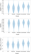 |
Fig. 11 Violin plots for the star formation properties. Top: SFE. Centre: DGF. Bottom: Clump luminosity-to-mass ratio (Lclump/Mclump) distributions for different morphologies. The violin plots present the density of the data at different values, which is smoothed through the kernel density estimator. The upper, lower, and middle horizontal lines in the plots represent the highest, lowest, and median values, respectively. |
P-values for the SFE.
p-values for DGF distributions of the cloud morphologies.
p-values for luminosity-to-mass ratio distributions of the cloud morphologies.
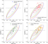 |
Fig. 12 HMSF threshold (dashed line; M[M⊙] = 1053 (R[pc])1.33) for molecular clouds using the MR (science) sample. The y axis represents M/Mcrit, where Mcrit = 1053 (R[pc])1.33 is the HMSF threshold. The coloured ellipses encompass approximately 99.7% of the data points and represent three-sigma levels for the cloud morphologies, which are indicated by the legends in the four plots. The clouds with HMSF tracers (Table 9) are denoted by a star (⋆). |
5.2.2 HMSF relation
The HMSF in clouds cannot be understood using a single cloud property and therefore, must be studied by relating different properties. Figure 12 shows the empirical relation between mass and radius for the various cloud morphologies. It highlights the HMSF threshold M[M⊙] = 1053 (R[pc])1.33, where M is the cloud mass and R is the deconvolved radius (DC2l). The threshold relation was initially obtained by Kauffmann & Pillai (2010) for dusty clumps, and was further updated by DC2l for the molecular clouds from the SEDIGISM survey.
The clouds above the HMSF threshold are expected to form high-mass stars. The original HMSF threshold (for clumps; Kauffmann & Pillai 2010) is a necessary but not a sufficient condition for HMSF, as it does not rule out the possibility for false positives. However, we see molecular clouds with star formation indicators (tracers) below the HMSF threshold, meaning they are false negatives (or missed true positives). It suggests that the HMSF threshold might not be suitable for our sample (discussed in details in DC2l). The errors in mass and radius estimations can also shift the positions of clouds with respect to the mass-radius relation (Fig. 12) and lead to false positives and negatives. Moreover, cloud radius (deconvolved radius from DC2l) might not effectively represent the size of a cloud with non-spherical geometry. We study the HMSF threshold as a follow-up on the cloud analysis of DC2l. We obtained the percentages of clouds above the threshold for different morphologies, and they are presented in Table 8. As we used the cloud radius, which requires reliable distance estimates for precise calculations, we used the clouds from the science sample (described in DC2l) to plot the HMSF relation. These clouds contain reliable distance estimates, are well resolved, and do not lie on the edge of the survey.
We find that none of the morphologies show a distinctly high percentage of HMSF clouds (Table 8). However, ringlike clouds and clumpy clouds show a comparatively higher percentage of HMSF clouds than the other two morphologies, and this is consistent with what is seen for the cloud SFEs in Sect. 5.2.1. Similarly, it is also seen that the clumpy clouds have a higher percentage of HMSF regions associated with them (using tracers mentioned in DC21) as compared to the elongated clouds (Table 9). We only consider the clouds with an ATLAS-GAL counterpart while calculating the percentage of clouds with HMSF tracer as these are a sub-sample of the ATLAS-GAL sources. The HMSF tracers (or signposts) include methanol masers, HII regions and young stellar objects from various surveys and are described in detail in DC21. The clouds with that host HMSF tracers are plotted with a star (⋆) in Fig. 12. The clouds with HMSF tracers typically lie above the mass-radius HMSF threshold for the different morphology, supporting the empirical relation.
The HMSF threshold (Kauffmann & Pillai 2010) provides evidence indicating a higher degree of star formation in ring-like clouds and clumpy clouds (Fig. 12). The number of clouds with HMSF regions belonging to these two morphologies is >16% for both the samples, as opposed to the lower values (<10%) for elongated and concentrated clouds (Table 8).
Percentage of clouds containing an HMSF tracer compared to the total clouds with an ATLASGAL clump (described in DC21) for the MR science sample (5020 clouds).
6 Summary
In this work we have classified molecular clouds from the SEDIGISM survey based on their morphology. This was achieved by using two classification methods. The first method – J plots – uses the moment of inertia of structures in the integrated intensity maps to classify them into three types. The second method – by-eye classification – visually classifies the clouds into four groups. The combined results from these two classifications result in the VC sample and the MR sample, which are used to affirm the reliability of the J plots classification. The VC sample (10365 clouds) is a subset of the full sample in which we exclude the unclassified clouds. The MR sample (8086 clouds) is a subset of the VC sample that contains only the clouds for which the morphologies are consistent for the two methods. We thus present the MR sample as our most reliable and robust sample, whereas the VC sample should be used when a larger sample size needs to be prioritised over the robustness of data.
We compared the positions of SEDIGISM molecular clouds with their sub-millimetre and infrared counterparts from two continuum surveys – ATLASGAL and MWP. We used the ATLASGAL survey to see how the elongated, lower-density SEDIGISM clouds compare to the dense dust continuum structures. The MWP was used to see how our ring-like clouds fare in comparison to the dust bubbles and stellar feedback regions. Almost all the AG-Els and more than 90% of the MWP bubbles in the SEDIGISM coverage have a molecular cloud counterpart. However, ≈64% of SEDIGISM clouds (the full sample) have neither an ATLASGAL nor an MWP counterpart. We find that 80% of the elongated clouds and 71% of the clumpy clouds in the MR sample lack an elongated ATLASGAL counterpart. The high percentage is in agreement with other findings in the literature since ATLASGAL traces high-density gas that is accompanied by low-density gas traced by SEDIGISM clouds, but not vice versa. There might also be sub-thermally excited gas traced by SEDIGISM that has a high column density but not a sufficiently high volume density to be detected by ATLASGAL in continuum. We also find that 66% of ring-like clouds lack an MWP bubble counterpart. MWP probes the HII and PAH regions, while SEDIGISM traces the molecular gas in the ISM, and thus a comparison between the column densities traced by the two surveys is complex. Large-scale shocks (HI flows) and supersonic turbulence could also lead to the creation of ring-like structures that are not detected at mid-infrared wavelengths.
We also studied the star formation activity for clouds in different morphology classes using two methods. The first method uses the SFEs and DGFs for SEDIGISM clouds obtained by Urquhart et al. (2021), and the second method uses the HMSF threshold (Kauffmann & Pillai 2010; DC21) for molecular clouds. These methods show that although none of the morphologies show very high star formation, ring-like and clumpy clouds show higher star formation when compared to elongated and concentrated clouds.
In conclusion, we have classified molecular clouds based on their morphology, and these morphologies show variations in star formation properties compared to the global cloud distribution. The various cloud morphologies closely resemble similar structures from other continuum surveys. Furthermore, ring-like clouds and especially clumpy clouds show evidence indicating higher star formation activity as compared to the other morphologies. A major observation across all the samples is that most of the molecular clouds are elongated. Finally, we also conclude that the automated cloud morphology classification based on J plots alone is not completely reliable.
Acknowledgements
The authors thank the referee for his/her valuable comments on the draft which helped improve the discussion of the paper and strengthened the results. This publication is based on data acquired with the Atacama Pathfinder Experiment (APEX) under programmes 092.F-9315 and 193.C-0584. APEX is a collaboration among the Max-Planck-Institut für Radioastronomie, the European Southern Observatory, and the Onsala Space Observatory. This publication uses data generated via the Zooniverse.org platform, development of which is funded by generous support, including a Global Impact Award from Google, and by a grant from the Alfred P. Sloan Foundation. A part of this work is based on observations made with the Spitzer Space Telescope, which is operated by the Jet Propulsion Laboratory, California Institute of Technology under a contract with NASA. D.C. acknowledges support by the German Deutsche Forschungsgemeinschaft, DFG project number SFB956A. A.D.C. acknowledges the support from the Royal Society University Research Fellowship (URF/R1/191609). H.B. acknowledges support from the European Research Council under the Horizon 2020 Framework Programme via the ERC Consol-idator Grant CSF-648505. H.B. also acknowledges support from the Deutsche Forschungsgemeinschaft in the Collaborative Research Center (SFB 881) “The Milky Way System” (subproject B1). C.L.D. acknowledges funding from the European Research Council for the Horizon 2020 ERC consolidator grant project ICYBOB, grant number 818940.
Appendix A Data products (catalogues)
We obtained the morphologies for the 10663 SEDIGISM molecular clouds and compiled them as a catalogue. The description for the columns in the catalogue is provided in Table A.1. It contains the structure of the clouds determined by the J plots (along with J moments) and by using by-eye classification. The table also mentions if a cloud is a part of the science, VC and MR samples. We also provide the number of overlapping structures from the ATLASGAL and MWP surveys (Sect. 5.1) for each SEDIGISM molecular cloud. These structures strictly fall in the SEDIGISM coverage, meaning they are excluded if they overlap with the survey edge (e.g. l = 18°). The complete catalogue of SEDIGISM molecular clouds (by DC21) is provided at https://sedigism.mpifr-bonn.mpg.de/index.html.
We also provide catalogues of the structures from ATLASGAL and MWP surveys that overlap with the SEDIGISM clouds. The ID numbers for the AG-Fil, AG-El (Li et al. 2016), and MWP bubbles (Jayasinghe et al. 2019) that overlap with the SEDIGISM clouds are provided in Tables A.2, A.3, and A.4, respectively.
Description of the generated catalogue that gives the morphology of molecular clouds and their overlapping counterparts.
Description of the AG-Fils that overlap with the SEDIGISM clouds.
Description of the AG-Els that overlap with the SEDIGISM clouds.
Description of the MWP bubbles that overlap with the SEDIGISM clouds.
Appendix B Overlap of SEDIGISM clouds with elongated ATLASGAL structures and MWP bubbles
We compare the SEDIGISM clouds with their counterparts from the ATLASGAL survey and MWP project. The figures B.1 – B.39 show the overlap between the SEDIGISM clouds, AG-El and MWP bubbles. ATLASGAL elongated structures consist of ‘filaments’, ‘networks of filaments’, and ‘resolved elongated structures’ (Li et al. 2016). The filaments are coloured red, networks of filaments are coloured blue and resolved elongated structures are coloured green. The black ellipses on the figure represent the MWP bubbles. These structures are overlaid on the SEDIGISM cloud masks of various colours and 13CO peak intensity in reverse grey scale. The catalogue for AG-El contains the position for each pixel in the structure whereas MWP bubble catalogue only contains the positions of the centres for the ellipses (bubbles) and their major and minor axes. Thus, our ellipses (Fig. B.1 – B.39) might not present the original structures of the actual bubbles, for example incomplete rings.
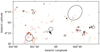 |
Fig. B.1 Elongated structures from the ATLASGAL survey (filaments in red, networks of filaments in blue, and resolved elongated structures in green) and bubbles (black ellipses) from the MWP survey overlaid on SEDIGISM clouds for 300° ≤ l ≤ 302°. |
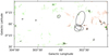 |
Fig. B.2 Elongated structures from the ATLASGAL survey and bubbles from the MWP survey overlaid on SEDIGISM clouds for 302° ≤ l ≤ 304°. |
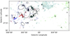 |
Fig. B.3 Elongated structures from the ATLASGAL survey and bubbles from the MWP survey overlaid on SEDIGISM clouds for 304° ≤ l ≤ 306°. |
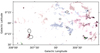 |
Fig. B.4 Elongated structures from the ATLASGAL survey and bubbles from the MWP survey overlaid on SEDIGISM clouds for 306° ≤ l ≤ 308°. |
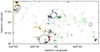 |
Fig. B.5 Elongated structures from the ATLASGAL survey and bubbles from the MWP survey overlaid on SEDIGISM clouds for 308° ≤ l ≤ 310°. |
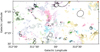 |
Fig. B.6 Elongated structures from the ATLASGAL survey and bubbles from the MWP survey overlaid on SEDIGISM clouds for 310° ≤ l ≤ 312°. |
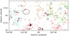 |
Fig. B.7 Elongated structures from the ATLASGAL survey and bubbles from the MWP survey overlaid on SEDIGISM clouds for 312° ≤ l ≤ 314°. |
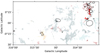 |
Fig. B.8 Elongated structures from the ATLASGAL survey and bubbles from the MWP survey overlaid on SEDIGISM clouds for 314° ≤ l ≤ 316°. |
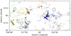 |
Fig. B.9 Elongated structures from the ATLASGAL survey and bubbles from the MWP survey overlaid on SEDIGISM clouds for 316° ≤ l ≤ 318°. |
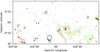 |
Fig. B.10 Elongated structures from the ATLASGAL survey and bubbles from the MWP survey overlaid on SEDIGISM clouds for 318° ≤ l ≤ 320°. |
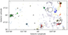 |
Fig. B.11 Elongated structures from the ATLASGAL survey and bubbles from the MWP survey overlaid on SEDIGISM clouds for 320° ≤ l ≤ 322°. |
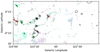 |
Fig. B.12 Elongated structures from the ATLASGAL survey and bubbles from the MWP survey overlaid on SEDIGISM clouds for 322° ≤ l ≤ 324°. |
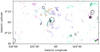 |
Fig. B.13 Elongated structures from the ATLASGAL survey and bubbles from the MWP survey overlaid on SEDIGISM clouds for 324° ≤ l ≤ 326°. |
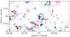 |
Fig. B.14 Elongated structures from the ATLASGAL survey and bubbles from the MWP survey overlaid on SEDIGISM clouds for 326° ≤ l ≤ 328°. |
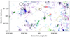 |
Fig. B.15 Elongated structures from the ATLASGAL survey and bubbles from the MWP survey overlaid on SEDIGISM clouds for 328° ≤ l ≤ 330°. |
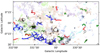 |
Fig. B.16 Elongated structures from the ATLASGAL survey and bubbles from the MWP survey overlaid on SEDIGISM clouds for 330° ≤ l ≤ 332°. |
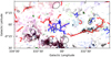 |
Fig. B.17 Elongated structures from the ATLASGAL survey and bubbles from the MWP survey overlaid on SEDIGISM clouds for 332° ≤ l ≤ 334°. |
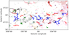 |
Fig. B.18 Elongated structures from the ATLASGAL survey and bubbles from the MWP survey overlaid on SEDIGISM clouds for 334° ≤ l ≤ 336°. |
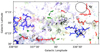 |
Fig. B.19 Elongated structures from the ATLASGAL survey and bubbles from the MWP survey overlaid on SEDIGISM clouds for 336° ≤ l ≤ 338°. |
 |
Fig. B.20 Elongated structures from the ATLASGAL survey and bubbles from the MWP survey overlaid on SEDIGISM clouds for 338° ≤ l ≤ 340°. |
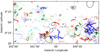 |
Fig. B.21 Elongated structures from the ATLASGAL survey and bubbles from the MWP survey overlaid on SEDIGISM clouds for 340° ≤ l ≤ 342°. |
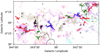 |
Fig. B.22 Elongated structures from the ATLASGAL survey and bubbles from the MWP survey overlaid on SEDIGISM clouds for 342° ≤ l ≤ 344°. |
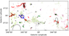 |
Fig. B.23 Elongated structures from the ATLASGAL survey and bubbles from the MWP survey overlaid on SEDIGISM clouds for 344° ≤ l ≤ 346°. |
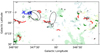 |
Fig. B.24 Elongated structures from the ATLASGAL survey and bubbles from the MWP survey overlaid on SEDIGISM clouds for 346° ≤ l ≤ 348°. |
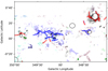 |
Fig. B.25 Elongated structures from the ATLASGAL survey and bubbles from the MWP survey overlaid on SEDIGISM clouds for 348° ≤ l ≤ 350°. |
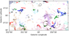 |
Fig. B.26 Elongated structures from the ATLASGAL survey and bubbles from the MWP survey overlaid on SEDIGISM clouds for 350° ≤ l ≤ 352°. |
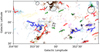 |
Fig. B.27 Elongated structures from the ATLASGAL survey and bubbles from the MWP survey overlaid on SEDIGISM clouds for 352° ≤ l ≤ 354°. |
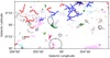 |
Fig. B.28 Elongated structures from the ATLASGAL survey and bubbles from the MWP survey overlaid on SEDIGISM clouds for 354° ≤ l ≤ 356°. |
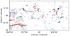 |
Fig. B.29 Elongated structures from the ATLASGAL survey and bubbles from the MWP survey overlaid on SEDIGISM clouds for 356° ≤ l ≤ 358°. |
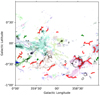 |
Fig. B.30 Elongated structures from the ATLASGAL survey and bubbles from the MWP survey overlaid on SEDIGISM clouds for 358° ≤ l ≤ 0°. |
 |
Fig. B.31 Elongated structures from the ATLASGAL survey and bubbles from the MWP survey overlaid on SEDIGISM clouds for 0° ≤ l ≤ 2°. |
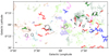 |
Fig. B.32 Elongated structures from the ATLASGAL survey and bubbles from the MWP survey overlaid on SEDIGISM clouds for 2° ≤ l ≤ 4°. |
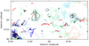 |
Fig. B.33 Elongated structures from the ATLASGAL survey and bubbles from the MWP survey overlaid on SEDIGISM clouds for 4° ≤ l ≤ 6°. |
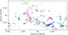 |
Fig. B.34 Elongated structures from the ATLASGAL survey and bubbles from the MWP survey overlaid on SEDIGISM clouds for 6° ≤ l ≤ 8°. |
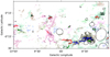 |
Fig. B.35 Elongated structures from the ATLASGAL survey and bubbles from the MWP survey overlaid on SEDIGISM clouds for 8° ≤ I ≤ 10°. |
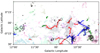 |
Fig. B.36 Elongated structures from the ATLASGAL survey and bubbles from the MWP survey overlaid on SEDIGISM clouds for 10° ≤ I ≤ 12°. |
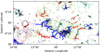 |
Fig. B.37 Elongated structures from the ATLASGAL survey and bubbles from the MWP survey overlaid on SEDIGISM clouds for 12° ≤ I ≤ 14°. |
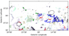 |
Fig. B.38 Elongated structures from the ATLASGAL survey and bubbles from the MWP survey overlaid on SEDIGISM clouds for 14° ≤ I ≤ 16°. |
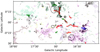 |
Fig. B.39 Elongated structures from the ATLASGAL survey and bubbles from the MWP survey overlaid on SEDIGISM clouds for 16° ≤ I ≤ 18°. |
Appendix C Original by-eye classification to morphological groups
Our original by-eye classification tried to follow the indication of the J plots algorithm – filaments, rings and cores. However, we realised that clouds in SEDIGISM sample showed repetitive patterns that would be better suited to six cloud morphologies. The first are bubbles. This category consists of clouds with a structure similar to a ring or a bubble. They have negligible elongation and resemble complete gas bubbles.
The second are filaments. These are elongated structures resolved along lengths and widths, with the lengths distinctly larger than the widths. They also show similar intensity across the entire length.
The third are cores. The centrally concentrated clouds without obvious elongations are classified as cores. These are molecular clouds and have no direct relation to pre-stellar and proto-stellar cores.
The fourth are elongated bubbles. This category consists of stretched bubbles, bubbles with filamentary structures attached to them, and clouds that resemble incomplete bubbles that form semi-circles.
The fifth are elongated cores. Elongated clouds with centrally concentrated structures are classified in this category.
The final category is multiple connected clouds (MCCs). Clouds that contain multiple dense regions belong to this category. They may be elongated structures similar to globular filaments. Clouds that do not resemble any of the above categories are listed as ‘unclassified.’
These sub-classes were merged to get four major morphological groups (Sect. 3.2). We renamed the four sub-classes – bubble, filament, core, and MCC – as ring-like, elongated, concentrated, and clumpy clouds, respectively. The remaining sub-classes were merged into the morphological groups using the two-sample KS test. The KS test was performed on the distributions of the seven properties: mass, surface density, radius, velocity dispersion, aspect ratio, virial parameter, and length. Based on the p-values from the KS test (Figs. C.1 and C.2), we classified the elongated bubbles as ring-like clouds and elongated cores as clumpy clouds.
We also conducted the two-sided MWU (Fay & Proschan 2010) test to compare the cloud properties distributions of elongated cores and elongated bubbles with other morphological sub-classes. The MWU test is a non-parametric test with a null hypothesis that neither distribution has stochastic dominance over other. It can be formally expressed as the probability of a variable drawn from a distribution ‘X’ having a greater value than a variable drawn from a distribution ‘Y’ being equal to the reverse (i.e. P(X > Y) = P(Y > X)). A high p-value would suggest that the two distributions are similar. An advantage of MWU test over the KS test is that it is not affected due to different widths of the distributions. The p-values obtained from our analysis (Fig. C.3) suggest a classification of elongated cores as clumpy clouds. The p-values for elongated bubbles (Fig. C.4) suggest that elongated bubbles have comparable distributions with both bubbles and MCC. However, a majority of the properties suggest that elongated bubbles have the closest distributions to bubbles. Thus, the morphological classes remain same as described by the KS test.
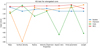 |
Fig. C.1 p-values obtained using a KS test on elongated cores and the four morphological sub-classes – bubbles, filaments, cores, and MCCs – for the various cloud properties. The different colours represent the morphologies that were compared with elongated cores to obtain the p-value. |
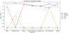 |
Fig. C.2 p-values obtained using a KS test on elongated bubbles and the four morphological sub-classes – bubbles, filaments, cores, and MCCs – for the various cloud properties. The different colours represent the morphologies that were compared with elongated bubbles to obtain the p-value. |
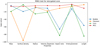 |
Fig. C.3 p-values obtained using an MWU test on elongated cores and the four morphological sub-classes – bubbles, filaments, cores, and MCCs – for the various cloud properties. The different colours represent the morphologies that were compared with elongated cores to obtain the p-value. |
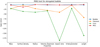 |
Fig. C.4 p-values obtained using an MWU test on elongated bubbles and the four morphological sub-classes – bubbles, filaments, cores, and MCCs – for the various cloud properties. The different colours represent the morphologies that were compared with elongated bubbles to obtain the p-value. |
References
- Abe, D., Inoue, T., Inutsuka, S.-I., & Matsumoto, T. 2021, ApJ, 916, 83 [NASA ADS] [CrossRef] [Google Scholar]
- Ali, A. A., & Harries, T. J. 2019, MNRAS, 487, 4890 [NASA ADS] [CrossRef] [Google Scholar]
- Ali, A. A., Bending, T. J. R., & Dobbs, C. L. 2022, MNRAS, 510, 5592 [NASA ADS] [CrossRef] [Google Scholar]
- André, P., Men'shchikov, A., Bontemps, S., et al. 2010, A&A, 518, L102 [CrossRef] [EDP Sciences] [Google Scholar]
- André, P., Di Francesco, J., Ward-Thompson, D., et al. 2014, in Protostars and Planets VI, eds. H. Beuther, R. S. Klessen, C. P. Dullemond, & T. Henning (Tucson: University of Arizona Press), 27 [Google Scholar]
- Arzoumanian, D. 2017, ArXiv e-prints [arXiv:1712.00604] [Google Scholar]
- Arzoumanian, D., Shimajiri, Y., Roy, A., et al. 2017, Mem. Soc. Astron. It., 88, 720 [Google Scholar]
- Arzoumanian, D., Shimajiri, Y., Inutsuka, S.-I., Inoue, T., & Tachihara, K. 2018, PASJ, 70, 96 [NASA ADS] [CrossRef] [Google Scholar]
- Arzoumanian, D., André, P., Könyves, V., et al. 2019, A&A, 621, A42 [NASA ADS] [CrossRef] [EDP Sciences] [Google Scholar]
- Balfour, S. K., Whitworth, A. P., Hubber, D. A., & Jaffa, S. E. 2015, MNRAS, 453, 2471 [Google Scholar]
- Beaumont, C. N., & Williams, J. P. 2010, ApJ, 709, 791 [NASA ADS] [CrossRef] [Google Scholar]
- Bending, T. J. R., Dobbs, C. L., & Bate, M. R. 2020, MNRAS, 495, 1672 [NASA ADS] [CrossRef] [Google Scholar]
- Benedettini, M., Traficante, A., Olmi, L., et al. 2021, A&A, 654, A144 [NASA ADS] [CrossRef] [EDP Sciences] [Google Scholar]
- Benjamin, R. A., Churchwell, E., Babler, B. L., et al. 2003, PASP, 115, 953 [Google Scholar]
- Bialy, S., Zucker, C., Goodman, A., et al. 2021, ApJ, 919, L5 [NASA ADS] [CrossRef] [Google Scholar]
- Bonne, L., Bontemps, S., Schneider, N., et al. 2020a, A&A, 644, A27 [EDP Sciences] [Google Scholar]
- Bonne, L., Schneider, N., Bontemps, S., et al. 2020b, A&A, 641, A17 [NASA ADS] [CrossRef] [EDP Sciences] [Google Scholar]
- Carey, D. 2016, Via Lactea Galactic Plane bubble Catalogue [Google Scholar]
- Carey, S., Ali, B., Berriman, B., et al. 2008, Spitzer Mapping of the Outer Galaxy (SMOG) (USA: Spitzer Proposal) [Google Scholar]
- Carey, S. J., Noriega-Crespo, A., Mizuno, D. R., et al. 2009, PASP, 121, 76 [Google Scholar]
- Churchwell, E., Povich, M. S., Allen, D., et al. 2006, ApJ, 649, 759 [CrossRef] [Google Scholar]
- Churchwell, E., Watson, D. F., Povich, M. S., et al. 2007, ApJ, 670, 428 [NASA ADS] [CrossRef] [Google Scholar]
- Churchwell, E., Babler, B. L., Meade, M. R., et al. 2009, PASP, 121, 213 [Google Scholar]
- Clarke, S. D., Whitworth, A. P., Duarte-Cabral, A., & Hubber, D. A. 2017, MNRAS, 468, 2489 [Google Scholar]
- Clarke, S. D., Williams, G. M., & Walch, S. 2020, MNRAS, 497, 4390 [NASA ADS] [CrossRef] [Google Scholar]
- Colombo, D., Rosolowsky, E., Ginsburg, A., Duarte-Cabral, A., & Hughes, A. 2015, MNRAS, 454, 2067 [NASA ADS] [CrossRef] [Google Scholar]
- Colombo, D., Rosolowsky, E., Duarte-Cabral, A., et al. 2019, MNRAS, 483, 4291 [NASA ADS] [CrossRef] [Google Scholar]
- Colombo, D., König, C., Urquhart, J. S., et al. 2021, A&A, 655, L2 [NASA ADS] [CrossRef] [EDP Sciences] [Google Scholar]
- Contreras, Y., Schuller, F., Urquhart, J. S., et al. 2013, A&A, 549, A45 [NASA ADS] [CrossRef] [EDP Sciences] [Google Scholar]
- Csengeri, T., Urquhart, J. S., Schuller, F., et al. 2014, A&A, 565, A75 [NASA ADS] [CrossRef] [EDP Sciences] [Google Scholar]
- Dale, J. E., Bonnell, I. A., Clarke, C. J., & Bate, M. R. 2005, MNRAS, 358, 291 [CrossRef] [Google Scholar]
- Dale, J. E., Ngoumou, J., Ercolano, B., & Bonnell, I. A. 2014, MNRAS, 442, 694 [Google Scholar]
- Deharveng, L., Zavagno, A., Schuller, F., et al. 2009, A&A, 496, 177 [NASA ADS] [CrossRef] [EDP Sciences] [Google Scholar]
- Deharveng, L., Schuller, F., Anderson, L. D., et al. 2010, A&A, 523, A6 [NASA ADS] [CrossRef] [EDP Sciences] [Google Scholar]
- Dobbs, C. L., & Wurster, J. 2021, MNRAS, 502, 2285 [NASA ADS] [CrossRef] [Google Scholar]
- Duarte-Cabral, A., & Dobbs, C. L. 2017, MNRAS, 470, 4261 [NASA ADS] [CrossRef] [Google Scholar]
- Duarte-Cabral, A., Colombo, D., Urquhart, J. S., et al. 2021, MNRAS, 500, 3027 [Google Scholar]
- Eden, D. J., Moore, T. J. T., Plume, R., & Morgan, L. K. 2012, MNRAS, 422, 3178 [NASA ADS] [CrossRef] [Google Scholar]
- Elmegreen, B. G., & Lada, C. J. 1977, ApJ, 214, 725 [Google Scholar]
- Fay, M., & Proschan, M. 2010, Stat. Surveys, 4, 1 [CrossRef] [Google Scholar]
- Francis, N., Boffin, H. M. J., Watkins, S. J., & Whitworth, A. P. 1998, ASP Conf. Ser., 132, 346 [NASA ADS] [Google Scholar]
- Fukui, Y., Inoue, T., Hayakawa, T., & Torii, K. 2021, PASJ, 73, S405 [Google Scholar]
- Fukushima, H., & Yajima, H. 2021, MNRAS, 506, 5512 [NASA ADS] [CrossRef] [Google Scholar]
- Geen, S., Hennebelle, P., Tremblin, P., & Rosdahl, J. 2015, MNRAS, 454, 4484 [NASA ADS] [CrossRef] [Google Scholar]
- Geen, S., Bieri, R., Rosdahl, J., & de Koter, A. 2021, MNRAS, 501, 1352 [Google Scholar]
- Grudic, M. Y., Kruijssen, J. M. D., Faucher-Giguère, C.-A., et al. 2021, MNRAS, 506, 3239 [NASA ADS] [CrossRef] [Google Scholar]
- Güsten, R., Nyman, L. Å., Schilke, P., et al. 2006, A&A, 454, L13 [NASA ADS] [CrossRef] [EDP Sciences] [Google Scholar]
- Habing, H. J., Israel, F. P., & de Jong, T. 1972, A&A, 17, 329 [NASA ADS] [Google Scholar]
- Haid, S., Walch, S., Seifried, D., et al. 2018, MNRAS, 478, 4799 [Google Scholar]
- Haid, S., Walch, S., Seifried, D., et al. 2019, MNRAS, 482, 4062 [NASA ADS] [CrossRef] [Google Scholar]
- Heitsch, F., Hartmann, L. W., Slyz, A. D., Devriendt, J. E. G., & Burkert, A. 2008, ApJ, 674, 316 [NASA ADS] [CrossRef] [Google Scholar]
- Hennebelle, P., Banerjee, R., Vázquez-Semadeni, E., Klessen, R. S., & Audit, E. 2008, A&A, 486, L43 [NASA ADS] [CrossRef] [EDP Sciences] [Google Scholar]
- Hora, J. L., Bontemps, S., Megeath, S. T., et al. 2009, AAS Meeting Abs., #213, 35601 [Google Scholar]
- Jackson, J. M., Finn, S. C., Chambers, E. T., Rathborne, J. M., & Simon, R. 2010, ApJ, 719, L185 [Google Scholar]
- Jaffa, S. E., Whitworth, A. P., Clarke, S. D., & Howard, A. D. P. 2018, MNRAS, 477, 1940 [NASA ADS] [CrossRef] [Google Scholar]
- Jayasinghe, T., Dixon, D., Povich, M. S., et al. 2019, MNRAS, 488, 1141 [NASA ADS] [CrossRef] [Google Scholar]
- Kauffmann, J., & Pillai, T. 2010, ApJ, 723, L7 [Google Scholar]
- Klessen, R. S., & Burkert, A. 2000, ApJS, 128, 287 [NASA ADS] [CrossRef] [Google Scholar]
- Könyves, V., André, P., & Maury, A. 2015, IAU General Assembly, 29, 2257481 [Google Scholar]
- Krumholz, M. R. 2006, ArXiv e-prints [arXiv:arXiv:astro-ph/0607429] [Google Scholar]
- Li, G.-X., Urquhart, J. S., Leurini, S., et al. 2016, A&A, 591, A5 [NASA ADS] [CrossRef] [EDP Sciences] [Google Scholar]
- Li, H., Vogelsberger, M., Marinacci, F., & Gnedin, O. Y. 2019, MNRAS, 487, 364 [NASA ADS] [CrossRef] [Google Scholar]
- Lin, L.-H., Wang, H.-C., Su, Y., Li, C., & Yang, J. 2020, Res. Astron. Astrophys., 20, 143 [CrossRef] [Google Scholar]
- Liow, K. Y., & Dobbs, C. L. 2020, MNRAS, 499, 1099 [NASA ADS] [CrossRef] [Google Scholar]
- Marsh, K. A., Kirk, J. M., André, P., et al. 2016, MNRAS, 459, 342 [Google Scholar]
- Mattern, M., Kainulainen, J., Zhang, M., & Beuther, H. 2018a, A&A, 616, A78 [NASA ADS] [CrossRef] [EDP Sciences] [Google Scholar]
- Mattern, M., Kauffmann, J., Csengeri, T., et al. 2018b, A&A, 619, A166 [NASA ADS] [CrossRef] [EDP Sciences] [Google Scholar]
- Mazumdar, P., Wyrowski, F., Colombo, D., et al. 2021, A&A, 650, A164 [NASA ADS] [CrossRef] [EDP Sciences] [Google Scholar]
- Molinari, S., Swinyard, B., Bally, J., et al. 2010, A&A, 518, L100 [NASA ADS] [CrossRef] [EDP Sciences] [Google Scholar]
- Nakamura, F., & Li, Z.-Y. 2008, ApJ, 687, 354 [NASA ADS] [CrossRef] [Google Scholar]
- Pabst, C. H. M., Goicoechea, J. R., Teyssier, D., et al. 2020, A&A, 639, A2 [NASA ADS] [CrossRef] [EDP Sciences] [Google Scholar]
- Padoan, P., Juvela, M., Goodman, A. A., & Nordlund, Å. 2001, ApJ, 553, 227 [NASA ADS] [CrossRef] [Google Scholar]
- Peretto, N., & Fuller, G. A. 2010, ApJ, 723, 555 [NASA ADS] [CrossRef] [Google Scholar]
- Pitts, R. L., Barnes, P. J., & Varosi, F. 2019, MNRAS, 484, 305 [NASA ADS] [CrossRef] [Google Scholar]
- Priestley, F. D., & Whitworth, A. P. 2022, MNRAS, 509, 1494 [Google Scholar]
- Ragan, S. E., Henning, T., Tackenberg, J., et al. 2014, A&A, 568, A73 [NASA ADS] [CrossRef] [EDP Sciences] [Google Scholar]
- Rosen, A. L., Offner, S. S. R., Sadavoy, S. I., et al. 2020, Space Sci. Rev., 216, 62 [Google Scholar]
- Rosolowsky, E., & Leroy, A. 2006, PASP, 118, 590 [NASA ADS] [CrossRef] [Google Scholar]
- Rosolowsky, E. W., Pineda, J. E., Kauffmann, J., & Goodman, A. A. 2008, ApJ, 679, 1338 [Google Scholar]
- Rosolowsky, E., Hughes, A., Leroy, A. K., et al. 2021, MNRAS, 502, 1218 [NASA ADS] [CrossRef] [Google Scholar]
- Schisano, E., Rygl, K. L. J., Molinari, S., et al. 2014, ApJ, 791, 27 [Google Scholar]
- Schisano, E., Molinari, S., Elia, D., et al. 2020, MNRAS, 492, 5420 [Google Scholar]
- Schneider, S., & Elmegreen, B. G. 1979, ApJS, 41, 87 [Google Scholar]
- Schneider, N., Simon, R., Guevara, C., et al. 2020, PASP, 132, 104301 [NASA ADS] [CrossRef] [Google Scholar]
- Schuller, F., Menten, K. M., Contreras, Y., et al. 2009, A&A, 504, 415 [NASA ADS] [CrossRef] [EDP Sciences] [Google Scholar]
- Schuller, F., Csengeri, T., Urquhart, J. S., et al. 2017, A&A, 601, A124 [NASA ADS] [CrossRef] [EDP Sciences] [Google Scholar]
- Schuller, F., Urquhart, J. S., Csengeri, T., et al. 2021, MNRAS, 500, 3064 [Google Scholar]
- Simpson, R. J., Povich, M. S., Kendrew, S., et al. 2012, MNRAS, 424, 2442 [NASA ADS] [CrossRef] [Google Scholar]
- Siringo, G., Kreysa, E., Kovács, A., et al. 2009, A&A, 497, 945 [NASA ADS] [CrossRef] [EDP Sciences] [Google Scholar]
- Suri, S., Sánchez-Monge, Á., Schilke, P., et al. 2019, A&A, 623, A142 [NASA ADS] [CrossRef] [EDP Sciences] [Google Scholar]
- Tiwari, M., Karim, R., Pound, M. W., et al. 2021, ApJ, 914, 117 [NASA ADS] [CrossRef] [Google Scholar]
- Urquhart, J. S., Csengeri, T., Wyrowski, F., et al. 2014, A&A, 568, A41 [NASA ADS] [CrossRef] [EDP Sciences] [Google Scholar]
- Urquhart, J. S., König, C., Giannetti, A., et al. 2018, MNRAS, 473, 1059 [Google Scholar]
- Urquhart, J. S., Figura, C., Cross, J. R., et al. 2021, MNRAS, 500, 3050 [Google Scholar]
- Urquhart, J. S., Wells, M. R. A., Pillai, T., et al. 2022, MNRAS, 510, 3389 [NASA ADS] [CrossRef] [Google Scholar]
- Vázquez-Semadeni, E., Banerjee, R., Gómez, G. C., et al. 2011, MNRAS, 414, 2511 [CrossRef] [Google Scholar]
- Wang, K., Testi, L., Ginsburg, A., et al. 2015, MNRAS, 450, 4043 [Google Scholar]
- Wang, Y., Bihr, S., Beuther, H., et al. 2020, A&A, 634, A139 [NASA ADS] [CrossRef] [EDP Sciences] [Google Scholar]
- Yuan, L., Yang, J., Du, F., et al. 2021, ApJS, 257, 51 [NASA ADS] [CrossRef] [Google Scholar]
- Zavagno, A., Deharveng, L., Comerón, F., et al. 2006, A&A, 446, 171 [NASA ADS] [CrossRef] [EDP Sciences] [Google Scholar]
- Zavagno, A., Anderson, L. D., Russeil, D., et al. 2010, A&A, 518, L101 [NASA ADS] [CrossRef] [EDP Sciences] [Google Scholar]
- Zhang, M., Kainulainen, J., Mattern, M., Fang, M., & Henning, T. 2019, A&A, 622, A52 [NASA ADS] [CrossRef] [EDP Sciences] [Google Scholar]
- Zhou, J., Zhou, D., Esimbek, J., et al. 2020, ApJ, 897, 74 [NASA ADS] [CrossRef] [Google Scholar]
- Zucker, C., Battersby, C., & Goodman, A. 2018, ApJ, 864, 153 [NASA ADS] [CrossRef] [Google Scholar]
We initially had six visual sub-classes, which were combined to get the current four classes. Complete and partial bubbles were combined to get the ring-like clouds. Elongated clouds with single and multiple denser clumps were combined to get clumpy clouds. A detailed description is provided in Appendix C.
These clouds look identical under the visual classification irrespective of the noise.
These represent the extreme values in the distribution, whereas ‘higher average values’ refer to an entire distribution that shows higher values for the given morphology.
All Tables
Number of overlapping clouds from the MR sample that lie completely inside SEDIGISM coverage (edge = 0; described in DC21).
Percentage of clouds containing an HMSF tracer compared to the total clouds with an ATLASGAL clump (described in DC21) for the MR science sample (5020 clouds).
Description of the generated catalogue that gives the morphology of molecular clouds and their overlapping counterparts.
All Figures
|
Fig. 1 Examples of two ring-like clouds as per the visual classification method. Left: J-bubble, cloud ID 238. Right: J-filament, cloud ID 3148. The cloud identification numbers (cloud IDs) can be used to identify the cloud structure from the main catalogue (Table A.1). The images are integrated intensity (moment 0) maps of the 13CO (2–1) transition. The numbers in the bottom-right corner of the images represent the J1 and the J2 moments, respectively. The colour bar represents the 13CO integrated intensity in K km s−1. The white contour represents the cloud edge. The white circle at the bottom left of the figure represents the telescope beam size. The black ellipse on the second image represents an artistic impression of the visualised ring. |
| In the text | |
|
Fig. 2 Examples of two elongated clouds as per the visual classification method. Left: J-filament, cloud ID 1726. Right: J-filament, cloud ID 130. The conventions follow Fig. 1. |
| In the text | |
|
Fig. 3 Examples of two concentrated clouds as per the visual classification method. Left: J-filament, cloud ID 3133. Right: J-core, cloud ID 6567. The conventions follow Fig. 1. |
| In the text | |
|
Fig. 4 Examples of two clumpy clouds as per the visual classification method. Left: J-filament, cloud ID 2500. Right: J-filament, cloud ID 3010. The conventions follow Fig. 1. |
| In the text | |
|
Fig. 5 Examples of two unclassified clouds. Left: J-filament, cloud ID 1445. Right: J-filament, cloud ID 3976. The conventions follow Fig. 1. |
| In the text | |
|
Fig. 6 J plot for the visual class ring-like clouds. The blue dots represent the ring-like clouds, and the grey dots represent all the clouds in VC sample. The blue dots lying inside the red dashed rectangle represent the MR sample. |
| In the text | |
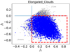 |
Fig. 7 J plot for the visual class elongated clouds. The symbols and conventions follow Fig. 6. |
| In the text | |
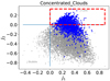 |
Fig. 8 J plot for the visual class concentrated clouds. The symbols and conventions follow Fig. 6. |
| In the text | |
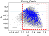 |
Fig. 9 J plot for the visual class clumpy clouds. The symbols and conventions follow Fig. 6. |
| In the text | |
|
Fig. 10 Comparison between aspect ratios obtained using the moment technique (ARmom) and the medial axis technique (ARma) for different cloud morphologies. The ellipses encompass approximately 95% of the respective data points (two-sigma level). The dashed black line represents the 1:1 relation. |
| In the text | |
|
Fig. 11 Violin plots for the star formation properties. Top: SFE. Centre: DGF. Bottom: Clump luminosity-to-mass ratio (Lclump/Mclump) distributions for different morphologies. The violin plots present the density of the data at different values, which is smoothed through the kernel density estimator. The upper, lower, and middle horizontal lines in the plots represent the highest, lowest, and median values, respectively. |
| In the text | |
|
Fig. 12 HMSF threshold (dashed line; M[M⊙] = 1053 (R[pc])1.33) for molecular clouds using the MR (science) sample. The y axis represents M/Mcrit, where Mcrit = 1053 (R[pc])1.33 is the HMSF threshold. The coloured ellipses encompass approximately 99.7% of the data points and represent three-sigma levels for the cloud morphologies, which are indicated by the legends in the four plots. The clouds with HMSF tracers (Table 9) are denoted by a star (⋆). |
| In the text | |
|
Fig. B.1 Elongated structures from the ATLASGAL survey (filaments in red, networks of filaments in blue, and resolved elongated structures in green) and bubbles (black ellipses) from the MWP survey overlaid on SEDIGISM clouds for 300° ≤ l ≤ 302°. |
| In the text | |
|
Fig. B.2 Elongated structures from the ATLASGAL survey and bubbles from the MWP survey overlaid on SEDIGISM clouds for 302° ≤ l ≤ 304°. |
| In the text | |
|
Fig. B.3 Elongated structures from the ATLASGAL survey and bubbles from the MWP survey overlaid on SEDIGISM clouds for 304° ≤ l ≤ 306°. |
| In the text | |
|
Fig. B.4 Elongated structures from the ATLASGAL survey and bubbles from the MWP survey overlaid on SEDIGISM clouds for 306° ≤ l ≤ 308°. |
| In the text | |
|
Fig. B.5 Elongated structures from the ATLASGAL survey and bubbles from the MWP survey overlaid on SEDIGISM clouds for 308° ≤ l ≤ 310°. |
| In the text | |
|
Fig. B.6 Elongated structures from the ATLASGAL survey and bubbles from the MWP survey overlaid on SEDIGISM clouds for 310° ≤ l ≤ 312°. |
| In the text | |
|
Fig. B.7 Elongated structures from the ATLASGAL survey and bubbles from the MWP survey overlaid on SEDIGISM clouds for 312° ≤ l ≤ 314°. |
| In the text | |
|
Fig. B.8 Elongated structures from the ATLASGAL survey and bubbles from the MWP survey overlaid on SEDIGISM clouds for 314° ≤ l ≤ 316°. |
| In the text | |
|
Fig. B.9 Elongated structures from the ATLASGAL survey and bubbles from the MWP survey overlaid on SEDIGISM clouds for 316° ≤ l ≤ 318°. |
| In the text | |
|
Fig. B.10 Elongated structures from the ATLASGAL survey and bubbles from the MWP survey overlaid on SEDIGISM clouds for 318° ≤ l ≤ 320°. |
| In the text | |
|
Fig. B.11 Elongated structures from the ATLASGAL survey and bubbles from the MWP survey overlaid on SEDIGISM clouds for 320° ≤ l ≤ 322°. |
| In the text | |
|
Fig. B.12 Elongated structures from the ATLASGAL survey and bubbles from the MWP survey overlaid on SEDIGISM clouds for 322° ≤ l ≤ 324°. |
| In the text | |
|
Fig. B.13 Elongated structures from the ATLASGAL survey and bubbles from the MWP survey overlaid on SEDIGISM clouds for 324° ≤ l ≤ 326°. |
| In the text | |
|
Fig. B.14 Elongated structures from the ATLASGAL survey and bubbles from the MWP survey overlaid on SEDIGISM clouds for 326° ≤ l ≤ 328°. |
| In the text | |
|
Fig. B.15 Elongated structures from the ATLASGAL survey and bubbles from the MWP survey overlaid on SEDIGISM clouds for 328° ≤ l ≤ 330°. |
| In the text | |
|
Fig. B.16 Elongated structures from the ATLASGAL survey and bubbles from the MWP survey overlaid on SEDIGISM clouds for 330° ≤ l ≤ 332°. |
| In the text | |
|
Fig. B.17 Elongated structures from the ATLASGAL survey and bubbles from the MWP survey overlaid on SEDIGISM clouds for 332° ≤ l ≤ 334°. |
| In the text | |
|
Fig. B.18 Elongated structures from the ATLASGAL survey and bubbles from the MWP survey overlaid on SEDIGISM clouds for 334° ≤ l ≤ 336°. |
| In the text | |
|
Fig. B.19 Elongated structures from the ATLASGAL survey and bubbles from the MWP survey overlaid on SEDIGISM clouds for 336° ≤ l ≤ 338°. |
| In the text | |
|
Fig. B.20 Elongated structures from the ATLASGAL survey and bubbles from the MWP survey overlaid on SEDIGISM clouds for 338° ≤ l ≤ 340°. |
| In the text | |
|
Fig. B.21 Elongated structures from the ATLASGAL survey and bubbles from the MWP survey overlaid on SEDIGISM clouds for 340° ≤ l ≤ 342°. |
| In the text | |
|
Fig. B.22 Elongated structures from the ATLASGAL survey and bubbles from the MWP survey overlaid on SEDIGISM clouds for 342° ≤ l ≤ 344°. |
| In the text | |
|
Fig. B.23 Elongated structures from the ATLASGAL survey and bubbles from the MWP survey overlaid on SEDIGISM clouds for 344° ≤ l ≤ 346°. |
| In the text | |
|
Fig. B.24 Elongated structures from the ATLASGAL survey and bubbles from the MWP survey overlaid on SEDIGISM clouds for 346° ≤ l ≤ 348°. |
| In the text | |
|
Fig. B.25 Elongated structures from the ATLASGAL survey and bubbles from the MWP survey overlaid on SEDIGISM clouds for 348° ≤ l ≤ 350°. |
| In the text | |
|
Fig. B.26 Elongated structures from the ATLASGAL survey and bubbles from the MWP survey overlaid on SEDIGISM clouds for 350° ≤ l ≤ 352°. |
| In the text | |
|
Fig. B.27 Elongated structures from the ATLASGAL survey and bubbles from the MWP survey overlaid on SEDIGISM clouds for 352° ≤ l ≤ 354°. |
| In the text | |
|
Fig. B.28 Elongated structures from the ATLASGAL survey and bubbles from the MWP survey overlaid on SEDIGISM clouds for 354° ≤ l ≤ 356°. |
| In the text | |
|
Fig. B.29 Elongated structures from the ATLASGAL survey and bubbles from the MWP survey overlaid on SEDIGISM clouds for 356° ≤ l ≤ 358°. |
| In the text | |
|
Fig. B.30 Elongated structures from the ATLASGAL survey and bubbles from the MWP survey overlaid on SEDIGISM clouds for 358° ≤ l ≤ 0°. |
| In the text | |
|
Fig. B.31 Elongated structures from the ATLASGAL survey and bubbles from the MWP survey overlaid on SEDIGISM clouds for 0° ≤ l ≤ 2°. |
| In the text | |
|
Fig. B.32 Elongated structures from the ATLASGAL survey and bubbles from the MWP survey overlaid on SEDIGISM clouds for 2° ≤ l ≤ 4°. |
| In the text | |
|
Fig. B.33 Elongated structures from the ATLASGAL survey and bubbles from the MWP survey overlaid on SEDIGISM clouds for 4° ≤ l ≤ 6°. |
| In the text | |
|
Fig. B.34 Elongated structures from the ATLASGAL survey and bubbles from the MWP survey overlaid on SEDIGISM clouds for 6° ≤ l ≤ 8°. |
| In the text | |
|
Fig. B.35 Elongated structures from the ATLASGAL survey and bubbles from the MWP survey overlaid on SEDIGISM clouds for 8° ≤ I ≤ 10°. |
| In the text | |
|
Fig. B.36 Elongated structures from the ATLASGAL survey and bubbles from the MWP survey overlaid on SEDIGISM clouds for 10° ≤ I ≤ 12°. |
| In the text | |
|
Fig. B.37 Elongated structures from the ATLASGAL survey and bubbles from the MWP survey overlaid on SEDIGISM clouds for 12° ≤ I ≤ 14°. |
| In the text | |
|
Fig. B.38 Elongated structures from the ATLASGAL survey and bubbles from the MWP survey overlaid on SEDIGISM clouds for 14° ≤ I ≤ 16°. |
| In the text | |
|
Fig. B.39 Elongated structures from the ATLASGAL survey and bubbles from the MWP survey overlaid on SEDIGISM clouds for 16° ≤ I ≤ 18°. |
| In the text | |
|
Fig. C.1 p-values obtained using a KS test on elongated cores and the four morphological sub-classes – bubbles, filaments, cores, and MCCs – for the various cloud properties. The different colours represent the morphologies that were compared with elongated cores to obtain the p-value. |
| In the text | |
|
Fig. C.2 p-values obtained using a KS test on elongated bubbles and the four morphological sub-classes – bubbles, filaments, cores, and MCCs – for the various cloud properties. The different colours represent the morphologies that were compared with elongated bubbles to obtain the p-value. |
| In the text | |
|
Fig. C.3 p-values obtained using an MWU test on elongated cores and the four morphological sub-classes – bubbles, filaments, cores, and MCCs – for the various cloud properties. The different colours represent the morphologies that were compared with elongated cores to obtain the p-value. |
| In the text | |
|
Fig. C.4 p-values obtained using an MWU test on elongated bubbles and the four morphological sub-classes – bubbles, filaments, cores, and MCCs – for the various cloud properties. The different colours represent the morphologies that were compared with elongated bubbles to obtain the p-value. |
| In the text | |
Current usage metrics show cumulative count of Article Views (full-text article views including HTML views, PDF and ePub downloads, according to the available data) and Abstracts Views on Vision4Press platform.
Data correspond to usage on the plateform after 2015. The current usage metrics is available 48-96 hours after online publication and is updated daily on week days.
Initial download of the metrics may take a while.