| Issue |
A&A
Volume 663, July 2022
|
|
|---|---|---|
| Article Number | A131 | |
| Number of page(s) | 29 | |
| Section | Galactic structure, stellar clusters and populations | |
| DOI | https://doi.org/10.1051/0004-6361/202243288 | |
| Published online | 21 July 2022 | |
An analysis of the most distant cataloged open clusters
Re-assessing fundamental parameters with Gaia EDR3 and ASteCA⋆
1
Instituto de Astrofísica de La Plata, IALP (CONICET-UNLP), 1900 La Plata, Argentina
e-mail: This email address is being protected from spambots. You need JavaScript enabled to view it.
2
Instituto de Física de Rosario, IFIR (CONICET-UNR), 2000 Rosario, Argentina
3
Facultad de Ciencias Exactas, Ingeniería y Agrimensura (UNR), 2000 Rosario, Argentina
4
Facultad de Ciencias Astronómicas y Geofísicas (UNLP), 1900 La Plata, Argentina
Received:
8
February
2022
Accepted:
24
March
2022
Abstract
Context. Several studies have been presented in the last few years applying some kind of automatic processing of data to estimate the fundamental parameters of open clusters. These parameters are then employed in larger scale analyses, for example the structure of the Galaxy’s spiral arms. The distance is one of the most straightforward parameters to estimate, yet enormous differences can still be found among published data. This is particularly true for open clusters located more than a few kiloparsecs away.
Aims. We cross-matched several published catalogs and selected the 25 most distant open clusters (> 9000 pc). We then performed a detailed analysis of their fundamental parameters, with emphasis on their distances, to determine the agreement between the catalogs and our estimates.
Methods. Photometric and astrometric data from the Gaia EDR3 survey was employed. The data were processed with our own membership analysis code, pyUPMASK, and our package for the automatic estimation of fundamental cluster parameters, ASteCA.
Results. We find differences in the estimated distances of up to several kiloparsecs between our results and those cataloged, even for the catalogs that show the best matches with ASteCA values. Large differences are also found for the age estimates. As a by-product of the analysis we find that vd Bergh-Hagen 176 could be the open cluster with the largest heliocentric distance cataloged to date.
Conclusions. Caution is thus strongly recommended when using cataloged parameters of open clusters to infer large-scale properties of the Galaxy, particularly for those located more than a few kiloparsecs away.
Key words: methods: statistical / galaxies: star clusters: general / open clusters and associations: general / techniques: photometric / astronomical databases: miscellaneous
Table 2 is only available at the CDS via anonymous ftp to cdsarc.u-strasbg.fr (130.79.128.5) or via http://cdsarc.u-strasbg.fr/viz-bin/cat/J/A+A/663/A131
© ESO 2022
1. Introduction
The unprecedented amount of high precision data for parallaxes, proper motions, and photometry provided by the Gaia mission in successive deliveries (DR2 and EDR3, Gaia Collaboration 2016, 2021b) offers us a unique opportunity to estimate the fundamental parameters of open clusters (OCs): metal content, age, total mass, binary fraction, distance, and extinction. The arrival of new techniques for analyzing massive quantities of data, combined with the increasing data precision, promises more reliable results than those obtained with the old techniques. The latter were mostly based on the visual inspection of their color–magnitude diagrams and isochrone fittings (Phelps & Janes 1994) or on direct comparison with HR diagrams of synthetic clusters (Siess et al. 1997). Automated processes such as that applied by Kharchenko et al. (2012) have also played a very important role in determining cluster parameters. The continuous increase of high quality data means that a variety of new analyses are being considered including artificial neural networks (Cantat-Gaudin et al. 2020), combined with new strategies for determining cluster memberships (Krone-Martins & Moitinho 2014; Cantat-Gaudin et al. 2018) or dynamical evolution analysis such as that applied by (Gregorio-Hetem et al. 2015).
The intrinsic value of studying OCs has been profusely described in several studies; we give here only a brief summary of the importance of these objects. The oldest OCs allow us to investigate the height and radial extension of the Galactic disk; old OCs tell us about the chemical history (age–metallicity relation), the mixing processes (radial metallicity gradient), and the processes of cluster destruction by interaction with other populations of the Galaxy (Friel 1995; Tosi et al. 2004; Lamers et al. 2005). The youngest OCs, on the other hand, are not only used as laboratories to investigate stellar evolution (they allow the boundary conditions necessary to create new generations of stars to be studied in detail; Lada & Lada 2003), but are also routinely employed in the analysis of the structure of the Milky Way (Loktin & Matkin 1992; Moitinho et al. 2006; Vázquez et al. 2008; Moitinho 2010) and are particularly useful in the tracing of spiral arms (Carraro 2013; Molina Lera et al. 2018).
Young OCs are arranged along the Galactic disk, where the strong visual absorption and the contamination by field stars very often prevent us from observing stars in the lower part of their main sequence. The situation is not much better for the older OCs which do not have very luminous stars in the main sequence, although they do in the giant branch. Stars in the lower part of the main sequences, as well as those belonging to the giant branch, share similar photometric characteristics with field stars making it rather difficult to unravel to which population each star belongs (Hayes et al. 2015).
The situation worsens as the distance to the older OCs increases because the limiting magnitude increases, which results in only a small portion of the lower part being visible. However, it is not only the photometric data dimensions that are disturbed by distance. The proper motions of distant OCs are extremely difficult to separate from those characterizing the field population against which we see them projected, therefore introducing an additional degree of confusion in determining memberships.
Our interest in this current topic is twofold. First, we focus on reexamining the distances and properties of the most distant OCs cataloged in our Galaxy. A total of 25 clusters that satisfy this requirement were found after inspecting four different recognized catalogs and databases, as we explain below. However, these catalogs display enormous differences in the estimated distances and ages. In part, these differences for the same cataloged object may be due to the varying techniques used to perform the analysis, combined with the problem of the very large distance at which they are located. We want to contribute to the task of resolving these differences.
Second, we want to test our new membership estimation technique pyUPMASK1 (Pera et al. 2021) in combination with the Automated Stellar Cluster Analysis (ASteCA) package2 (Perren et al. 2015) on clusters with proper motions not easily distinguishable from those of surrounding stars, and that are composed of a small number of members and with non-trivial sequences in the photometric space.
This article is structured as follows. In Sect. 2 we introduce the stellar cluster catalogs, the clusters selected to be analyzed (cross-matched from those catalogs), and the photometric and astrometric data used to perform the analysis. Section 3 presents the methods employed in the study of all the clusters. The comparison of the estimated parameters with the cataloged values for each cluster is done in Sect. 4. Finally, our conclusions are highlighted in Sect. 5.
2. Catalogs, clusters, and data
We selected four catalogs to cross-match and subsequently use to identify the most distant clusters: Dias et al. (2002, the New Catalog of Optically Visible Open Clusters and Candidates, hereafter OC02); Netopil et al. (2012, hereafter WEBDA3); Kharchenko et al. (2012, Milky Way Star Clusters Catalog, hereafter MWSC); and Cantat-Gaudin et al. (2020, hereafter CG20).
The first two (OC02 and WEBDA) are compilations of open cluster fundamental parameters from the literature. They contain around 1700 (WEBDA) and 2100 (OC02) entries, and are heavily used in the field of open cluster research. The parameter values in the two catalogs are heterogeneous, being compiled from various sources. The MWSC catalog is the largest (∼3000 entries) and, similarly to the CG20 catalog (∼2000 entries), is composed of homogeneous fundamental parameter values obtained for all its entries. The method employed by the authors of the MWSC catalog is a semi-automated isochrone fit applied on clusters and candidate clusters, while the CG20 catalog was generated employing an artificial neural network only on verified clusters (trained on parameter values taken from the literature).
Since we are interested in the open clusters most distant from the Sun, we select from these cross-matched catalogs those that are located at a distance of 9000 pc or more in either of them. This is an arbitrary value that results in enough clusters to draw general conclusions, but not too many that would impede their detailed analysis. The final 25 clusters that were studied in this work are shown in Table 1.
Selected open clusters with a cataloged distance ≥9000 pc, ordered by right ascension.
Our full list initially consisted of 38 open clusters, 11 of which were found only in the MWSC catalog with distances greater than 9000 pc. These clusters are either listed with substantially smaller distances in the other catalogs, or were too sparse and/or dubious, and were thus removed from the cross-matched list.
Two other clusters were also removed from the initial list: Shorlin 1 (α2000 = 166.44, δ2000 = −61.23) and FSR0338 (α2000 = 327.93, δ2000 = 55.33). The latter appears in WEBDA and MWSC at a distance of 12 600 pc and 5600 pc, respectively, while the former is listed only in MWSC at a distance of 14 655 pc. Shorlin1 is studied in Carraro & Costa (2009) and Turner (2012); in both cases the authors conclude that this is not a real cluster, but a grouping of young stars. FSR0338 is analyzed in Froebrich et al. (2010) where a distance of 6000 pc is assigned, but with large uncertainties. In both cases we find no evidence of a true stellar cluster in these regions. We base our conclusion on two findings: the large proper motion dispersion of the stars that occupy the overdensity around the central coordinates assigned to either object and the lack of a clear sequence in their respective color-magnitude diagrams (CMDs). These two clusters were thus also discarded from further analysis.
Most of the 25 selected clusters are located in the third quadrant; all of them are in the latitude range of [−12°,8°], relatively close to the Galactic plane. The final list thus contains 24 clusters present in the MWSC catalog, 21 in WEBDA, 19 in OC02, and 16 in CG20.
There are two other major works where a large catalog of analyzed open clusters is presented: Liu & Pang (2019) and Dias et al. (2021). The former does not contain clusters with such large distances, and was not used. The latter lists only four clusters that are also present in our set of 25 selected clusters. None of their distances meet the criteria of our selection filter, hence this database was not included. Nevertheless, their distance values are mentioned in the discussion of the results in Sect. 4.
Data from Gaia EDR3 (Gaia Collaboration 2016, 2021b) were retrieved for a box of 20 arcmin in length around the central coordinates for all the clusters. We employed equatorial coordinates, parallax, proper motions, and photometry (G, GBP − GRP) from this survey. In Fig. 1 we show the 25 selected clusters for each of the four catalogs, positioned on the face-on view of the Galaxy (top), and two edge-on views (center, bottom). The spiral arms are those presented in Momany et al. (2006). The large dispersion for the distances assigned to each cluster in different catalogs is clearly visible, where ideally the position of all the clusters would overlap for the four catalogs.
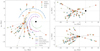 |
Fig. 1. Position of the 25 clusters selected from the four catalogs mentioned in the text. Left: face-on view of the Milky Way. The Sun and the center of the Galaxy are shown as a yellow filled circle and a black filled circle, respectively. Right, top and bottom: same as left, but for edge-on views. The sight lines are shown in gray for each cluster. |
In what follows we only show the figures for a single representative cluster (Berkeley 29) to avoid clutter and to improve the readability of the article. The plots for the remaining clusters can be found in the appendix.
3. Cluster analysis
3.1. Structural analysis
The first step in the cluster analysis is the estimation of their structural properties (i.e., center coordinates and limiting radius). Although the centers and diameters are present in some of the catalogs, not all of these values are correct. We use our ASteCA package throughout this work to perform the structural and fundamental parameters analysis. We applied this tool to the study of hundreds of clusters in previous articles, with excellent results (Perren et al. 2017, 2020).
The center values are obtained applying a two-dimensional kernel density analysis (KDE) on each of the cluster’s coordinates. This method assigns the center of the cluster to the point with the highest density in the frame. As shown in previous articles (Perren et al. 2015, 2017, 2020), this approach is robust even when applied on frames with star densities that are highly non-uniform (see, e.g., the case of van den Bergh-Hagen 37 in Fig. A.4).
A King’s profile fit (King 1962) is performed on the radial density profile (RDP) of each cluster to estimate their core and tidal radii (rc, rt). The adopted radius ra is the limiting distance from the center used to define the studied cluster region for each cluster. These radii are estimated applying a process that compares the ratio of the approximated number of true members for increasing radii values with the number of stars in a concentric ring centered on each radius. The approximated number of members is obtained as the total number of stars within the radius, minus the expected number (field density times circle area). This method produces an overdensity around the value where the radial density approaches the field density, maximizing the contrast between members included within the radius and contaminating field stars. The method is also useful for heavily contaminated clusters and/or clusters with very few true members. All radius values are shown in Table A.1.
The adopted radius ra is on average 50% smaller than the tidal radius (see Table A.1). This allows us to reduce the field star contamination, while ensuring that only a small number of true members (cluster stars located as far from the center as the tidal radius) are lost. The fraction of lost members can be estimated integrating King’s profile. This fraction depends on the concentration of the cluster (rt/rc) and the value of the adopted radius as a fraction of the tidal radius (ra/rt). In our case, less than 20% of the members could be lost in a worst-case scenario. Since these are clusters that are strongly contaminated (particularly in the parallax and proper motion spaces), the trade-off between losing a small portion of members and improving the contrast of the true members over the field noise is positive. Because the ra values used in our analysis are smaller than the tidal radius, the total estimated mass for each cluster shown in Sect. 4 must be thought of as a lower limit.
In Fig. 2 we show the structural analysis and the center and radius estimation processes for the cluster Berkeley 29. The plots for the remaining clusters can be seen in Appendix A.
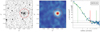 |
Fig. 2. Structural analysis for the cluster Berkeley 29. Left: analyzed 20′×20′ arcmin frame with the estimated cluster region enclosed in a red circle. Asterisks in the equatorial coordinates of the left plot indicate that these were shifted and transformed so that the center of the frame is located at (0, 0) and to remove projection artifacts. Center: same frame, but shown as a 2D density map. Right: radial density analysis, axis shown in logarithmic scale. The dashed green line and the shaded green area are the King profile fit and its 16th–84th uncertainty region, respectively. The green dotted vertical line, solid red vertical line, and solid green vertical line are respectively the core (rc), adopted (ra), and tidal (rt) radii. The dashed and dotted horizontal black lines are the field density estimate and its ±1σ region, respectively. |
3.2. Membership and fundamental parameters
Before we can estimate the fundamental parameters with ASteCA, we needed to select the set of most probable members for each cluster. For this task we employed our recently developed pyUPMASK algorithm which performed very well for very contaminated clusters, even outperforming UPMASK (Krone-Martins & Moitinho 2014), as shown in Pera et al. (2021). Internal tests showed that pyUPMASK also outperforms ASteCA’s own membership algorithm, hence the reason why we selected the former over the latter.
pyUPMASk requires an input data set composed of (α, δ) coordinates and at least two dimensions of data of any type to estimate the membership probabilities. We chose to make use of the proper motion data dimensions only, thus excluding photometric and parallax data. We made the decision to leave out these extra data dimensions because, although they can sometimes be useful in the process of singling out the most probable members, for this type of very distant clusters they tend to add more noise than information. This is particularly true for the parallax data which rapidly tends to zero for stars beyond ∼2 kpc, where the parallax values for the cluster members become almost indistinguishable from the contaminating field stars. The selected clustering method in pyUPMASK is a Gaussian mixture model, which was demonstrated to have the best performance in Pera et al. (2021, see Sect. 4).
Once pyUPMASK has assigned membership probabilities to all the stars in the frame, we must select the stars that most likely belong to the cluster (i.e., true members). This selection is performed within the cluster region, defined as r ≤ ra, where r is the distance to the cluster center. This step is usually handled by selecting an arbitrary cutoff probability value; in Cantat-Gaudin et al. (2020), for example, the authors fix this value to P = 70%. Instead of setting an ad hoc value, we performed an analysis that combines the membership probabilities with the stellar density inside and outside the cluster region. This allowed us to estimate the number of cluster members expected within the cluster region. Combining this number with the membership probabilities given by pyUPMASK we selected those stars with the highest probabilities within the cluster region, such that the resulting total number of members was as close as possible to the expected number (i.e., that obtained through the stellar density analysis).
Using a physically reasonable number of members not only reduces the probability of excluding true members (by only selecting those with the highest membership probabilities), it also ensures that the estimation of the total mass parameter is properly performed by ASteCA.
After selecting the set of true members for all the clusters as described above, we fed this data directly to the final section of our ASteCA package bypassing its internal membership algorithm. The goal of this section is to estimate the fundamental parameters: metallicity, age, total mass, fraction of binary systems, distance, and extinction. The code uses the ptemcee parallel tempering Bayesian inference algorithm (Vousden et al. 2016) to sample the distributions of the fundamental parameters. The likelihood function employed to assess the fit between the observed cluster and the synthetic clusters is the Bayesian Poisson ratio defined in Tremmel et al. (2013). The theoretical isochrones used to generate the synthetic clusters used to match the observed clusters are the PARSEC tracks (Bressan et al. 2012). Priors are uniform for all the parameters using the following limiting ranges:
-
metallicity ([Fe/H]): [−0.60, 0.30];
-
logarithmic age: [8, 10.1];
-
total mass: [1e2, 2e5] M⊙;
-
binarity fraction: [0, 1];
-
distance modulus: [10, 20] mag;
-
EBV extinction: [0,
 ].
].
The maximum value for the extinction priors,  , was set on a per cluster basis selecting the values given by the Schlegel et al. (1998) extinction maps with the re-calibration by Schlafly & Finkbeiner (2011). The logarithmic abundances [Fe/H] were obtained using the approximation given in the CMD service for [M/H]4 given that the PARSEC isochrones are generated using Z.
In Fig. 3 we show the result of the membership probabilities estimation done with pyUPMASK, plus the fundamental parameter estimation performed by ASteCA. We only show here the plots for the cluster Berkeley 29; the remaining clusters can be seen in Appendix B. The plot on the left shows the vector point diagram (VPD) with the proper motion distributions for both the selected clusters members, and the field stars. The members are clearly very much embedded within the field star distribution, which is expected for distant clusters. The center plot shows the CMD traced by the selected members, and the right plot a sampling of the best fit synthetic cluster. The grid in the center and right plots is the two-dimensional binning used to estimate the likelihood, obtained using Knuth’s rule (Knuth 2006). The gray region represents the uncertainty in the fit. The isochrone drawn in the center and right plots is associated with the synthetic cluster, but it is there merely to guide the eye; the fit is performed for the CMD of the observed cluster versus the CMD of synthetic clusters, not versus theoretical isochrones (this is further explained in Perren et al. 2015, 2017, 2020).
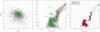 |
Fig. 3. Estimation of the membership probabilities and the fundamental parameters for the cluster Berkeley 29. Left: VPD for stars in the analyzed Berkeley 29 frame. The green and gray circles show the selected true members and the field stars, respectively. Center: CMD for the cluster members with the isochrone associated with the best synthetic cluster fit drawn in red to guide the eye. Right: Best synthetic cluster fit found by ASteCA with the same isochrone, now show in green. The blue and red circles are single and binary systems, respectively. |
4. Results and discussion
We present the general results for the fundamental parameters contrasted with values taken from the above-mentioned databases, with particular emphasis on the distances.
In Appendix C we discuss each cluster individually, commenting on the most relevant studies published in the literature and how these compare to the results obtained in this article.
Henceforth we employ the default values for the galactocentric coordinate frame given by the astropy package5:
-
ICRS coordinates of the Galactic center: (266.4051°, −28.936175°);
-
Distance from the sun to the Galactic center: 8.122 pc;
-
Distance from the sun to the Galactic midplane: 20.8 pc;
-
Velocity of the sun in the galactocentric frame as Cartesian velocity components: (12.9, 245.6, 7.78) km s−1.
Table 2 shows the fundamental parameters along with their uncertainties estimated by ASteCA. The Bayesian inference process was allowed to run for enough steps to achieve convergence.
Fundamental parameters estimated with ASteCA for the 25 analyzed clusters.
In Fig. 4 we show how the map of the Galaxy shown in Fig. 1 looks, but with the distance parameter values found in this work. The arrows represent the velocity vectors for all the clusters with available radial velocity. The sizes correspond to the estimated masses, and the colors follow the distribution of ages, metallicities, and binary fraction as shown in the color bars to the right of each plot. The values used to construct this figure are presented in Table D.1. It is worth noting that only about half of the clusters are truly beyond the 9 kpc (∼14.8 mag) limit originally used to perform the selection from the published databases.
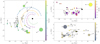 |
Fig. 4. Same as Fig. 1, but showing the positions given by our analysis with ASteCA. The velocity vectors are drawn for those clusters with available radial velocities. The length of the vectors are proportional to the velocity modules in each 2D projection. Sizes follow masses and colors follow ages, metallicities, and binary fractions for the left, top right, and bottom right plots, respectively. |
The cluster vd Bergh-Hagen 176, located in the fourth quadrant in Fig. 4, turns out to be the most distant open cluster cataloged to date with a heliocentric distance greater than 18 kpc. Its status as a bona fide open cluster is nonetheless still questioned; a more detailed discussion is presented in Appendix C.
In a recent study (Anders et al. 2022) per star parameters such as distance, extinction, metallicity, and age were estimated. Comparing the results from this analysis with those from Cantat-Gaudin et al. (2020), the authors find differences in the distance values larger than 3 kpc for clusters located at 6 kpc or more from the Sun. We find even larger discrepancies between our analysis and those taken from the four databases. As shown in Fig. 5, all but the CG20 database show differences of up to 10 kpc for clusters spanning the full distance range. The CG20 database, the one with the better overall match to our values, only shows differences larger than 2 kpc for clusters located beyond ∼10 kpc from the Sun. Taking the uncertainties of both estimates into account, these differences are expected; particularly for such distant clusters.
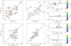 |
Fig. 5. ASteCA vs. database distances. The plots to the right stacked vertically are the ASteCA distances vs. the differences in the sense (ASteCA – database). Clusters are colored according to the log age assigned by ASteCA. |
We see no evident trend that correlates the differences in the distance with the ages (used to color the symbols in the right plots of Fig. 5).
To further investigate the various ways to estimate the distance, we performed two more analyses. First, we re-ran ASteCA for all the clusters using four different combinations of settings for the metallicity and binary fraction parameters. We chose these two parameters because in isochrone-fit analyses they are usually either fixed (e.g., the metallicity is set to solar) or neglected altogether (e.g., the binary fraction).
Second, we compared the distances estimated in this work with those obtained via parallax analysis using three different methods: ASteCA’s own Bayesian inference estimation (described in Perren et al. 2020), the distance inferred by the Kalkayotl package (Olivares et al. 2020), and the median of a simple inversion of the parallax values of the selected members. The parallax values were previously corrected using the method described in Lindegren et al. (2021)6.
The results of these two extra analyses can be seen in Fig. 6 compared to the main ASteCA run (i.e., the one whose estimated parameter values are shown in Table 2). In the top plot we show the variation in the distance estimates between our main ASteCA run and four different runs: metallicity fixed to solar and binary fraction fixed to 0 (Z = Z⊙, bfr = 0.0; blue left facing triangles); metallicity fixed to solar and binary fraction as a free parameter (Z = Z⊙; green right facing triangles); metallicity as a free parameter and binary fraction fixed to 0 (bfr = 0.0; orange squares); and metallicity fixed to solar and binary fraction fixed to 0.5 (Z = Z⊙, bfr = 0.5; red diamonds), where 50% is chosen to be a typical estimate for binary fraction in open clusters (von Hippel 2005). The median difference with the main ASteCA run is largest when the binary fraction is fixed to 0.0 (∼1100 pc), smaller when we fix this parameter to 0.5 (∼100 pc), and smallest when it is allowed to vary (∼50 pc). This is another indicator that a proper binary fraction fit is of utmost importance for a correct estimation of the cluster’s fundamental parameters, particularly for the distance. Even when the binary fraction is free, fixing just the metallicity to solar values can have a non-negligible impact on the estimated distances, as shown in Fig. 6 (green right facing triangles).
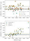 |
Fig. 6. Distances obtained by the main run of ASteCA compared to other configurations and methods. In both plots the abscissa is the main run ASteCA distance values and the ordinate shows the difference in the sense (ASteCA – ASteCA*), where the asterisk represents either of the four runs from the top plot or either method from the bottom plot. In both plots the black dashed line indicates zero difference and the colored dotted lines the median differences for each run. Top: main run distances vs. four different runs where the metallicity and binary fraction were either fixed or allowed to be fitted. Bottom: main run distances vs. the difference with the distances estimated using parallax values and three different methods. |
The bottom plot in Fig. 6 shows the parallax value analysis. Here the distance estimates obtained by ASteCA processing the Gaia EDR3 photometry are compared to three methods to estimate distances using parallaxes: ASteCA’s own Bayesian inference, the Kalkayotl package estimate, and the inversion of the median of the selected member’s parallaxes. It is clear that a trend arises where the most distant clusters have their distances enormously underestimated by any of the parallax-based methods. This is expected as the parallax values of the most distant clusters are associated with very large uncertainties and are also heavily affected by noise from non-removed field stars that mostly contaminate the lower mass region. It is surprising to see that the naive approach of inverting the median of the member’s parallaxes is the method that most closely approximates the photometric distances estimated by ASteCA: the mean difference is only ∼600 pc, where the other two methods show median differences more that twice as large (∼1200 pc).
All the analyzed clusters are rather old; the youngest one (vd Bergh-Hagen 37) has an assigned age of ∼0.7 Gyr, although we note the very large uncertainty associated with it.
The comparisons between our age estimation and those from the four databases are shown in Fig. 7. The top plot shows that ASteCA systematically assigns ages that are older on average than those from the databases. A logarithmic difference of ∼0.23 dex (the average value for all the catalogs) translates to a difference of ∼1.5 Gyr for an age of 3 Gyr, which is a reasonable uncertainty given the complexities associated with the clusters under investigation. The catalog with the smallest logarithmic difference is CG20 with a median of 0.11 dex, again displaying the best match to the values given by ASteCA.
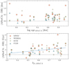 |
Fig. 7. ASteCA ages vs. ages from the four databases. Top: differences in logarithmic ages between ASteCA and the databases in the sense (ASteCA – database). The cluster Kronberger 39 was left out of the plot to improve visibility. Bottom: linear age differences vs. binarity fraction assigned by ASteCA. The blue dashed line is the regression trend. |
The largest age difference arises for Kronberger 39, for which ASteCA finds an age of log(age) = 9.45, but has an age of log(age) = 6 assigned in the MWSC database (the youngest age by far in the four databases).
As can be seen in the bottom plot of Fig. 7, there appears to be a slight correlation between the difference in age estimates and the binarity fractions. The trend shows that the higher the percentage of binary systems present in the cluster, the larger on average the difference between the age value obtained by ASteCA and those in the databases. This effect can be explained by noticing that the TO in the CMD is pushed downward by the presence of binaries, which are located above the brightest point of the main sequence of single stars. This in turn forces the fit to adjust toward older ages, hence producing the systematic trend seen in the analysis. This result points to the importance of taking binary systems into account when performing stellar clusters’ parameter estimations.
The metal content of a cluster is the hardest parameter to estimate photometrically, which is why it is usually fixed to solar value in this type of analysis. We found six clusters from our sample that are also investigated spectroscopically in very recent works: Berkeley 25, Berkeley 29, Berkeley 73, Czernik 30, Saurer 1, and Tombaugh 2 studied in Donor et al. (2020), Netopil et al. (2022), and Spina et al. (2021). The abundances are shown in Table 3 along with the ASteCA estimates. Uncertainties are around 0.02, 0.06, and 0.04 dex for Donor et al. (2020), Netopil et al. (2022), and Spina et al. (2021), respectively. The uncertainties associated with the ASteCA values are substantially larger, averaging 0.2 dex (see Table 2).
Six cluster from our sample whose [Fe/H] metal content is also analyzed in recent works.
In Fig. 8 we show the metallicity vs. galactocentric distance (RGC) distribution for the clusters in our sample, plus ten verified clusters from Perren et al. (2020). This distribution (also called radial metallicity distribution or metallicity gradient) is a key tracer of the Galaxy’s chemical evolution. Open clusters have been used as a tool to investigate this relation for several decades (Janes 1979). The gradient is usually taken to be around −0.05 dex kpc−1 for the inner clusters, with a break beyond RGC ≈ 10 kpc into a shallower slope (Donor et al. 2020). In Donor et al. (2018) it is shown that the metallicity gradient is also (as expected) highly dependent on the database used fix the distances, varying by as much as 40% depending on the database used. This result was confirmed in Donor et al. (2020), where a database-dependent variation of 15% was found.
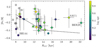 |
Fig. 8. Metallicity gradient for the set of 25 analyzed clusters. Points are colored according to the log(age). The gray vertical lines are the 16th and 84th percentiles. The dotted line is the broken relation from Donor et al. (2020, Fig. 7). The gray dots are the ten verified clusters from Perren et al. (2020). |
We see in Fig. 8 that ASteCA assigns on average a slightly higher metallicity (∼0.06 dex) than that expected for clusters located below RGC ≈ 14 kpc.
The case of vd Bergh-Hagen 144 is interesting because its estimated metallicity of ![Mathematical equation: $ \mathrm{[Fe/H]}=-0.53_{-0.48}^{-0.55} $](/articles/aa/full_html/2022/07/aa43288-22/aa43288-22-eq178.gif) is well below the expected solar value at that distance (RGC ∼ 8.5 kpc). There are two other articles where a similar markedly sub-solar metallicity was found for this cluster: Frinchaboy et al. (2006b) and Fragkou et al. (2019). In these studies the reported metallicity values are [Fe/H] = −0.51 ± 0.3 (spectroscopic metallicity from two stars) and [Fe/H] ≈ −0.40 (photometric estimate)7 for Frinchaboy et al. (2004) and Fragkou et al. (2019), respectively.
is well below the expected solar value at that distance (RGC ∼ 8.5 kpc). There are two other articles where a similar markedly sub-solar metallicity was found for this cluster: Frinchaboy et al. (2006b) and Fragkou et al. (2019). In these studies the reported metallicity values are [Fe/H] = −0.51 ± 0.3 (spectroscopic metallicity from two stars) and [Fe/H] ≈ −0.40 (photometric estimate)7 for Frinchaboy et al. (2004) and Fragkou et al. (2019), respectively.
Fragkou et al. (2019) assigned a distance of 12 ± 0.5 kpc, ∼4 kpc larger than that found by ASteCA, while in Frinchaboy et al. (2004) the estimated distance is 9.35 kpc, which is a much closer value to ours.
For the seven clusters beyond this galactocentric distance the difference with ASteCA is larger, where our code assigns abundances on average 0.20 dex above the Donor et al. gradient. Saurer 1 is the cluster with the largest value in this group, with an abundance assigned by ASteCA of ![Mathematical equation: $ \mathrm{[Fe/H]}= -0.08_{-0.34}^{0.16} $](/articles/aa/full_html/2022/07/aa43288-22/aa43288-22-eq179.gif) , which conflicts with the value ∼ − 0.42 dex expected for its galactocentric distance.
, which conflicts with the value ∼ − 0.42 dex expected for its galactocentric distance.
There are several articles where this cluster was assigned a markedly sub-solar [Fe/H] value: −0.27 (Carraro & Baume 2003), −0.38 ± 0.14 (Carraro et al. 2004), −0.50 (Frinchaboy et al. 2004), −0.38 (Frinchaboy et al. 2006a), −0.42 ± 0.01 (Donor et al. 2020). The distances given to Saurer 1 in these studies are located in the range [12, 13.2] kpc, a reasonable match for the distance estimated by ASteCA of  kpc. It is thus clear that ASteCA has overestimated the metal content for this cluster. Saurer 1 is the third oldest cluster in our sample (∼6.6 Gyr) and one of the most distant from the Sun, which results in less than a full magnitude visible below the TO with a total of only 84 members present in the CMD. This is very likely the reason for the large difference in the abundance estimated by ASteCA versus the value predicted by the radial metallicity trend and the spectroscopic analyses.
The clusters analyzed in Perren et al. (2020) on the other hand (shown as gray circles in the plot) display a much more balanced distribution around the [Fe/H] ≈ 0.0 dex expected value for their galactocentric distance of ∼9 kpc.
The abundances presented here should therefore be taken with caution. It is always preferable to refer to spectroscopic estimates whenever available, particularly when dealing with very distant, old, scarcely populated, and/or heavily contaminated clusters.
The assigned binary fractions range from 32% to ∼86%, with a mean value of 63% for the entire sample. Although this value is not that far off from the typical value expected for open clusters (50%, as stated previously), it is a bit high. On the other hand, the uncertainties are also rather large and the binary fractions assigned to most of the clusters drop below 50% within their 1σ range. In Sollima et al. (2010) the binary fraction within the core radius of five clusters is estimated. The authors find values in the range 35%–70% with a combined mean value of 56%, somewhat similar to ours. We did not estimate core binary fractions, but we did employ radii about 50% smaller than the cluster’s tidal radii, so the large binarity found could be related to this. In any case, as these are rather distant and old clusters, most of which have a very small portion of their sequence observed, these values should also be used with caution.
The total estimated masses are found in the range [2000, 60 000] M⊙ with the exception of vd Bergh-Hagen 176, for which a much higher mass of ∼170 000 M⊙ is given. This is a high mass value for an open cluster, which would suggest that this object is closer to being classified as a young globular cluster. It is worth noting that these are lower limit mass estimates since ASteCA does not take into account the experienced dynamical mass loss, which can be significant for old stellar clusters (Martinez-Medina et al. 2017).
5. Conclusions
Taking advantage of the precise photometry and proper motions from the most recent Gaia data release (Gaia Collaboration 2021b), the fundamental parameters of the 25 most distant cataloged clusters (> 9 kpc) have been reassessed using pyUPMASK and ASteCA. The results for the fundamental parameters of metallicity, age, distance, extinction, total mass, and binary fraction are shown in Table 2. In this table we can see that these are rather old clusters: with the exception of just two (vd Bergh-Hagen 37 and Kronberger 31) the remaining clusters are all older than 1 Gyr. Only 13 clusters out of 25 turn out to be at a distance greater than 9 kpc from the Sun, thus reducing the number of clusters that fit the minimum distance criterion by almost half.
Regarding the distribution in the Galactic plane and the galactocentric distance, we see that 14 clusters are placed in the third Galactic quadrant, 10 of which with negative latitudes and thus located below the formal Galactic equator. The remaining four clusters that are above the Galactic plane are Berkeley 26 (Z ≈ 0.2 kpc), Saurer 1 (Z ≈ 1.6 kpc), Czernik 30 (Z ≈ 0.5 kpc), and Berkeley 29 (Z ≈ 2 kpc). The cluster with the largest galactocentric distance, Berkeley 29, is also the cluster with the largest vertical distance. This cluster is on its course to cross the Galactic disk, as shown by its velocity vector seen in Fig. 4. Maximum vertical distances of ∼1.8 kpc for Berkeley 29 and ∼1.6 kpc for Saurer 1 are estimated in Gaia Collaboration (2021a). These values are in reasonable agreement with the vertical distances obtained here, meaning that both clusters are currently at their maximum height above the Galactic plane.
Despite some bias effect (e.g., lower dust absorption, particularly along the Fitzgerald window; Fitzgerald 1968), it appears that a large number of clusters in the third quadrant of the Galaxy follow the warp defined by the diffuse blue population (Carraro et al. 2005c; Moitinho et al. 2006), whose maximum height above the Galactic equator is located at about [lat = −8°, lon = 240°].
The four databases list 14 clusters with galactocentric distances larger than 15 kpc (in either one of them), the assumed limit for the Galactic disk radius (see Carraro et al. 2010, and references therein). One of the most relevant results emerging from our new distance estimation is that five clusters were confirmed to be located beyond this value: Tombaugh 2 (RGC ≈ 15.1 kpc), Arp-Madore 2 (RGC ≈ 15.8 kpc), FSR 1212 (RGC ≈ 16.7 kpc), Saurer 1 (RGC ≈ 19.6 kpc), and Berkeley 29 (RGC ≈ 22.2 kpc). These values are in line with recent findings where evidence of populations more than 15 kpc away from the Galactic center was presented (Liu et al. 2017; López-Corredoira et al. 2018, and references therein).
In this work we reported distant open clusters (older tan 1.2 Gyr) instead of single stars, as shown in most of the papers referred to above. A recent review of the spatial distribution of star clusters and the impact of the subsequent releases of Gaia data on the topic can be found in Cantat-Gaudin (2022).
When comparing the results given by our analysis with ASteCA with those present in the MWSC, WEBDA, and OC02 databases, we clearly see substantial disagreements in age and distance (the fundamental parameters available in these catalogs). The best overall agreement in distances, the main objective of this article, is found with the database presented in CG20. For the 16 clusters in common with this work the differences range from −2 to +3 kpc, without any apparent dependency on the ages. Within the limits of the uncertainties associated with the distance parameter, we can say that the agreement with CG20 is good. The differences with other databases are substantially larger, spanning a range from −10 to +10 kpc, and are present in the case of MWSC and WEBDA for clusters whose cataloged distance is even below 5 kpc. The age parameter also suffers from important inconsistencies, with the best match found again with the CG20 catalog. Caution is hence advised when making use of these databases for large-scale analyses. We thus recommend choosing the CG20 database over the rest whenever possible.
Assuming [M/H] ∼ [Fe/H], [Fe/H] = log(Z/X)−log(Z/X)o, where (Z/X)o = 0.0207; Y = 0.2485 + 1.78Z. CMD service: http://stev.oapd.inaf.it/cgi-bin/cmd
Analytical functions to compute the expected parallax zero-point as a function of ecliptic latitude, magnitude, and color for any Gaia (e)DR3 source: https://gitlab.com/icc-ub/public/gaiadr3_zeropoint
Transformed from the fitted Z = 0.006 assuming Z⊙ = 0.0152.
The distance modulus value of 16.07 mag quoted in Table 7 of Hayes et al. is incorrect. The proper value is ∼14.5 mag, as shown in Table 7 of Perren et al. (2015).
Acknowledgments
We are grateful for the suggestions and comments given by the referee, which greatly improved the final version of this paper. G.I.P., M.S.P., and R.A.V. acknowledge the financial support from CONICET (PIP317) and the UNLP (PID-G148 project). This work has made use of data from the European Space Agency (ESA) mission Gaia (https://www.cosmos.esa.int/gaia), processed by the Gaia Data Processing and Analysis Consortium (DPAC, https://www.cosmos.esa.int/web/gaia/dpac/consortium). Funding for the DPAC has been provided by national institutions, in particular the institutions participating in the Gaia Multilateral Agreement. This research has made use of the WEBDA database, operated at the Department of Theoretical Physics and Astrophysics of the Masaryk University. This research has made use of the VizieR catalog access tool, operated at CDS, Strasbourg, France (Ochsenbein et al. 2000). This research has made use of “Aladin sky atlas” developed at CDS, Strasbourg Observatory, France (Bonnarel et al. 2000; Boch & Fernique 2014). This research has made use of NASA’s Astrophysics Data System. This research made use of the Python language v3.7.3 (van Rossum 1995) and the following packages: NumPy (http://www.numpy.org/) (Van Der Walt et al. 2011); SciPy (http://www.scipy.org/) (Jones et al. 2001); Astropy (http://www.astropy.org/), a community-developed core Python package for Astronomy (Astropy Collaboration 2013, 2018); matplotlib (http://matplotlib.org/) (Hunter 2007); scikit-learn (https://scikit-learn.org/) (Pedregosa et al. 2011); ASteCA (https://github.com/asteca); ptemcee (https://github.com/willvousden/ptemcee); Kalkayotl (https://github.com/olivares-j/Kalkayotl); sfdmap (https://github.com/kbarbary/sfdmap).
References
- Anders, F., Khalatyan, A., Queiroz, A. B. A., et al. 2022, A&A, 658, A91 [NASA ADS] [CrossRef] [EDP Sciences] [Google Scholar]
- Astropy Collaboration (Robitaille, T. P., et al.) 2013, A&A, 558, A33 [NASA ADS] [CrossRef] [EDP Sciences] [Google Scholar]
- Astropy Collaboration (Price-Whelan, A. M., et al.) 2018, AJ, 156, 123 [Google Scholar]
- Bica, E., Ortolani, S., & Barbuy, B. 1999, A&AS, 136, 363 [NASA ADS] [CrossRef] [EDP Sciences] [Google Scholar]
- Boch, T., & Fernique, P. 2014, in Astronomical Data Analysis Software and Systems XXIII, eds. N. Manset, & P. Forshay, ASP Conf. Ser., 485, 277 [NASA ADS] [Google Scholar]
- Bonnarel, F., Fernique, P., Bienaymé, O., et al. 2000, A&AS, 143, 33 [NASA ADS] [CrossRef] [EDP Sciences] [Google Scholar]
- Bressan, A., Marigo, P., Girardi, L., et al. 2012, MNRAS, 427, 127 [NASA ADS] [CrossRef] [Google Scholar]
- Cantat-Gaudin, T. 2022, Universe, 8, 111 [NASA ADS] [CrossRef] [Google Scholar]
- Cantat-Gaudin, T., Jordi, C., Vallenari, A., et al. 2018, A&A, 618, A93 [NASA ADS] [CrossRef] [EDP Sciences] [Google Scholar]
- Cantat-Gaudin, T., Anders, F., Castro-Ginard, A., et al. 2020, A&A, 640, A1 [NASA ADS] [CrossRef] [EDP Sciences] [Google Scholar]
- Carraro, G. 2013, Proc. Int. Astron. Union, 9, 7 [NASA ADS] [CrossRef] [Google Scholar]
- Carraro, G., & Baume, G. 2003, MNRAS, 346, 18 [Google Scholar]
- Carraro, G., & Costa, E. 2007, A&A, 464, 573 [NASA ADS] [CrossRef] [EDP Sciences] [Google Scholar]
- Carraro, G., & Costa, E. 2009, A&A, 493, 71 [NASA ADS] [CrossRef] [EDP Sciences] [Google Scholar]
- Carraro, G., Vallenari, A., & Ortolani, S. 1995, A&A, 300, 128 [NASA ADS] [Google Scholar]
- Carraro, G., Bresolin, F., Villanova, S., et al. 2004, AJ, 128, 1676 [Google Scholar]
- Carraro, G., Geisler, D., Moitinho, A., Baume, G., & Vázquez, R. A. 2005a, A&A, 442, 917 [NASA ADS] [CrossRef] [EDP Sciences] [Google Scholar]
- Carraro, G., Janes, K. A., & Eastman, J. D. 2005b, MNRAS, 364, 179 [NASA ADS] [CrossRef] [Google Scholar]
- Carraro, G., Vázquez, R. A., Moitinho, A., & Baume, G. 2005c, ApJ, 630, L153 [NASA ADS] [CrossRef] [Google Scholar]
- Carraro, G., Subramaniam, A., & Janes, K. A. 2006, MNRAS, 371, 1301 [NASA ADS] [CrossRef] [Google Scholar]
- Carraro, G., Geisler, D., Villanova, S., Frinchaboy, P. M., & Majewski, S. R. 2007, A&A, 476, 217 [NASA ADS] [CrossRef] [EDP Sciences] [Google Scholar]
- Carraro, G., Vázquez, R. A., Costa, E., Perren, G., & Moitinho, A. 2010, ApJ, 718, 683 [Google Scholar]
- Carraro, G., Beletsky, Y., & Marconi, G. 2013, MNRAS, 428, 502 [NASA ADS] [CrossRef] [Google Scholar]
- Davoust, E., Sharina, M. E., & Donzelli, C. J. 2011, A&A, 528, A70 [NASA ADS] [CrossRef] [EDP Sciences] [Google Scholar]
- Dias, W. S., Alessi, B. S., Moitinho, A., & Lépine, J. R. D. 2002, A&A, 389, 871 [NASA ADS] [CrossRef] [EDP Sciences] [Google Scholar]
- Dias, W. S., Alessi, B. S., Moitinho, A., & Lepine, J. R. D. 2007, VizieR Online Data Catalog: B/ocl [Google Scholar]
- Dias, W. S., Monteiro, H., Moitinho, A., et al. 2021, MNRAS, 504, 356 [NASA ADS] [CrossRef] [Google Scholar]
- Donor, J., Frinchaboy, P. M., Cunha, K., et al. 2018, AJ, 156, 142 [NASA ADS] [CrossRef] [Google Scholar]
- Donor, J., Frinchaboy, P. M., Cunha, K., et al. 2020, AJ, 159, 199 [NASA ADS] [CrossRef] [Google Scholar]
- Fitzgerald, M. P. 1968, AJ, 73, 983 [NASA ADS] [CrossRef] [Google Scholar]
- Fragkou, V., Parker, Q. A., Zijlstra, A., Shaw, R., & Lykou, F. 2019, MNRAS, 484, 3078 [Google Scholar]
- Friel, E. D. 1995, ARA&A, 33, 381 [Google Scholar]
- Frinchaboy, P. M., & Phelps, R. L. 2002, AJ, 123, 2552 [Google Scholar]
- Frinchaboy, P. M., Majewski, S. R., Crane, J. D., et al. 2004, ApJ, 602, L21 [Google Scholar]
- Frinchaboy, P. M., Muñoz, R. R., Phelps, R. L., Majewski, S. R., & Kunkel, W. E. 2006a, AJ, 131, 922 [NASA ADS] [CrossRef] [Google Scholar]
- Frinchaboy, P. M., Muñoz, R. R., Majewski, S. R., et al. 2006b, Chemical Abundances and Mixing in Stars in the Milky Way and its Satellites, 130 [CrossRef] [Google Scholar]
- Frinchaboy, P. M., Marino, A. F., Villanova, S., et al. 2008, MNRAS, 391, 39 [NASA ADS] [CrossRef] [Google Scholar]
- Froebrich, D., Scholz, A., & Raftery, C. L. 2007, MNRAS, 374, 399 [Google Scholar]
- Froebrich, D., Schmeja, S., Samuel, D., & Lucas, P. W. 2010, MNRAS, 409, 1281 [NASA ADS] [CrossRef] [Google Scholar]
- Gaia Collaboration (Prusti, T., et al.) 2016, A&A, 595, A1 [NASA ADS] [CrossRef] [EDP Sciences] [Google Scholar]
- Gaia Collaboration (Antoja, T., et al.) 2021a, A&A, 649, A8 [EDP Sciences] [Google Scholar]
- Gaia Collaboration (Brown, A. G. A., et al.) 2021b, A&A, 649, A1 [NASA ADS] [CrossRef] [EDP Sciences] [Google Scholar]
- Gregorio-Hetem, J., Hetem, A., Santos-Silva, T., & Fernandes, B. 2015, MNRAS, 448, 2504 [NASA ADS] [CrossRef] [Google Scholar]
- Harris, W. E. 1996, AJ, 112, 1487 [Google Scholar]
- Harris, W. E. 2010, ArXiv e-prints [arXiv:1012.3224] [Google Scholar]
- Hasegawa, T., Sakamoto, T., & Malasan, H. L. 2008, PASJ, 60, 1267 [NASA ADS] [CrossRef] [Google Scholar]
- Hayes, C. R., Friel, E. D., Slack, T. J., & Boberg, O. M. 2015, AJ, 150, 200 [NASA ADS] [CrossRef] [Google Scholar]
- Hunter, J. D., et al. 2007, Comput. Sci. Eng., 9, 90 [NASA ADS] [CrossRef] [Google Scholar]
- Janes, K. A. 1979, ApJS, 39, 135 [NASA ADS] [CrossRef] [Google Scholar]
- Janes, K. A., & Hoq, S. 2011, AJ, 141, 92 [NASA ADS] [CrossRef] [Google Scholar]
- Janes, K. A., & Phelps, R. L. 1994, AJ, 108, 1773 [NASA ADS] [CrossRef] [Google Scholar]
- Jones, E., Oliphant, T., Peterson, P., et al. 2001, SciPy: Open Source Scientific Tools for Python [Online; accessed 2016–06-21] [Google Scholar]
- Kharchenko, N. V., Piskunov, A. E., Schilbach, E., Röser, S., & Scholz, R. D. 2012, A&A, 543, A156 [NASA ADS] [CrossRef] [EDP Sciences] [Google Scholar]
- King, I. 1962, AJ, 67, 471 [Google Scholar]
- King, I. R. 1964, Royal Greenwich Obs. Bullet., 82, 106 [NASA ADS] [Google Scholar]
- Knuth, K. H. 2006, ArXiv e-prints [arXiv:physics/0605197] [Google Scholar]
- Kronberger, M., Teutsch, P., Alessi, B., et al. 2006, A&A, 447, 921 [NASA ADS] [CrossRef] [EDP Sciences] [Google Scholar]
- Krone-Martins, A., & Moitinho, A. 2014, A&A, 561, A57 [NASA ADS] [CrossRef] [EDP Sciences] [Google Scholar]
- Kubiak, M. 1991, Acta Astron., 41, 231 [NASA ADS] [Google Scholar]
- Kubiak, M., Kaluzny, J., Krzeminski, W., & Mateo, M. 1992, Acta Astron., 42, 155 [NASA ADS] [Google Scholar]
- Lada, C. J., & Lada, E. A. 2003, ARA&A, 41, 57 [Google Scholar]
- Lamers, H. J. G. L. M., Gieles, M., Bastian, N., et al. 2005, A&A, 441, 117 [NASA ADS] [CrossRef] [EDP Sciences] [Google Scholar]
- Lee, M. G. 1997, AJ, 113, 729 [NASA ADS] [CrossRef] [Google Scholar]
- Lindegren, L., Bastian, U., Biermann, M., et al. 2021, A&A, 649, A4 [EDP Sciences] [Google Scholar]
- Liu, C., Xu, Y., Wan, J.-C., et al. 2017, Res. Astron. Astrophys., 17, 096 [Google Scholar]
- Liu, L., & Pang, X. 2019, ApJS, 245, 32 [NASA ADS] [CrossRef] [Google Scholar]
- Loktin, A. V., & Matkin, N. V. 1992, Astron. Astrophys. Trans., 3, 169 [NASA ADS] [CrossRef] [Google Scholar]
- López-Corredoira, M., Allende Prieto, C., Garzón, F., et al. 2018, A&A, 612, L8 [EDP Sciences] [Google Scholar]
- Maciejewski, G., & Niedzielski, A. 2008, Astron. Nach., 329, 602 [NASA ADS] [CrossRef] [Google Scholar]
- Majaess, D., Carraro, G., Moni Bidin, C., et al. 2014, A&A, 567, A1 [Google Scholar]
- Martinez-Medina, L. A., Pichardo, B., Peimbert, A., & Moreno, E. 2017, ApJ, 834, 58 [Google Scholar]
- Moitinho, A., Vázquez, R. A., Carraro, G., et al. 2006, MNRAS, 368, L77 [NASA ADS] [CrossRef] [Google Scholar]
- Moitinho, A. 2010, in Star Clusters: Basic Galactic Building Blocks Throughout Time and Space, eds. R. de Grijs, & J. R. D. Lépine, IAU Symp., 266, 106 [Google Scholar]
- Molina Lera, J. A., Baume, G., & Gamen, R. 2018, MNRAS, 480, 2386 [NASA ADS] [CrossRef] [Google Scholar]
- Momany, Y., Zaggia, S., Gilmore, G., et al. 2006, A&A, 451, 515 [NASA ADS] [CrossRef] [EDP Sciences] [Google Scholar]
- Monteiro, H., Dias, W. S., Moitinho, A., et al. 2020, MNRAS, 499, 1874 [NASA ADS] [CrossRef] [Google Scholar]
- Netopil, M., Paunzen, E., & Stütz, C. 2012, in Star Clusters in the Era of Large Surveys, eds. A. Moitinho, & J. Alves (Berlin, Heidelberg: Springer), 53 [CrossRef] [Google Scholar]
- Netopil, M., Oralhan, İ. A., Çakmak, H., Michel, R., & Karataş, Y. 2022, MNRAS, 509, 421 [Google Scholar]
- Ochsenbein, F., Bauer, P., & Marcout, J. 2000, A&AS, 143, 23 [NASA ADS] [CrossRef] [EDP Sciences] [Google Scholar]
- Olivares, J., Sarro, L. M., Bouy, H., et al. 2020, A&A, 644, A7 [NASA ADS] [CrossRef] [EDP Sciences] [Google Scholar]
- Ortolani, S., Bica, E., & Barbuy, B. 1995, A&A, 300, 726 [NASA ADS] [Google Scholar]
- Ortolani, S., Bica, E., Barbuy, B., & Zoccali, M. 2005, A&A, 439, 1135 [NASA ADS] [CrossRef] [EDP Sciences] [Google Scholar]
- Ortolani, S., Bica, E., & Barbuy, B. 2008, MNRAS, 388, 723 [NASA ADS] [CrossRef] [Google Scholar]
- Parker, Q. A., Frew, D. J., Miszalski, B., et al. 2011, MNRAS, 413, 1835 [NASA ADS] [CrossRef] [Google Scholar]
- Pedregosa, F., Varoquaux, G., Gramfort, A., et al. 2011, J. Mach. Learn. Res., 12, 2825 [Google Scholar]
- Pera, M. S., Perren, G. I., Moitinho, A., Navone, H. D., & Vazquez, R. A. 2021, A&A, 650, A109 [NASA ADS] [CrossRef] [EDP Sciences] [Google Scholar]
- Perren, G. I., Vázquez, R. A., & Piatti, A. E. 2015, A&A, 576, A6 [NASA ADS] [CrossRef] [EDP Sciences] [Google Scholar]
- Perren, G. I., Piatti, A. E., & Vázquez, R. A. 2017, A&A, 602, A89 [NASA ADS] [CrossRef] [EDP Sciences] [Google Scholar]
- Perren, G. I., Giorgi, E. E., Moitinho, A., et al. 2020, A&A, 637, A95 [NASA ADS] [CrossRef] [EDP Sciences] [Google Scholar]
- Phelps, R. L., & Janes, K. A. 1994, ApJS, 90, 31 [NASA ADS] [CrossRef] [Google Scholar]
- Phelps, R. L., & Schick, M. 2003, AJ, 126, 265 [NASA ADS] [CrossRef] [Google Scholar]
- Phelps, R. L., Janes, K. A., & Montgomery, K. A. 1994, AJ, 107, 1079 [NASA ADS] [CrossRef] [Google Scholar]
- Piatti, A. E., Clariá, J. J., & Ahumada, A. V. 2010, MNRAS, 402, 2720 [NASA ADS] [CrossRef] [Google Scholar]
- Salaris, M., Weiss, A., & Percival, S. M. 2004, A&A, 414, 163 [NASA ADS] [CrossRef] [EDP Sciences] [Google Scholar]
- Saurer, W., Seeberger, R., Weinberger, R., & Ziener, R. 1994, AJ, 107, 2101 [NASA ADS] [CrossRef] [Google Scholar]
- Schlafly, E. F., & Finkbeiner, D. P. 2011, ApJ, 737, 103 [Google Scholar]
- Schlegel, D. J., Finkbeiner, D. P., & Davis, M. 1998, ApJ, 500, 525 [Google Scholar]
- Sharina, M. E., Donzelli, C. J., Davoust, E., Shimansky, V. V., & Charbonnel, C. 2014, A&A, 570, A48 [NASA ADS] [CrossRef] [EDP Sciences] [Google Scholar]
- Siess, L., Forestini, M., & Dougados, C. 1997, A&A, 324, 556 [NASA ADS] [Google Scholar]
- Sollima, A., Carballo-Bello, J. A., Beccari, G., et al. 2010, MNRAS, 401, 577 [NASA ADS] [CrossRef] [Google Scholar]
- Soubiran, C., Cantat-Gaudin, T., Romero-Gómez, M., et al. 2018, A&A, 619, A155 [NASA ADS] [CrossRef] [EDP Sciences] [Google Scholar]
- Spina, L., Ting, Y. S., De Silva, G. M., et al. 2021, MNRAS, 503, 3279 [CrossRef] [Google Scholar]
- Tadross, A. L. 2008, MNRAS, 389, 285 [NASA ADS] [CrossRef] [Google Scholar]
- Tarricq, Y., Soubiran, C., Casamiquela, L., et al. 2021, A&A, 647, A19 [NASA ADS] [CrossRef] [EDP Sciences] [Google Scholar]
- Tosi, M., Di Fabrizio, L., Bragaglia, A., Carusillo, P. A., & Marconi, G. 2004, MNRAS, 354, 225 [Google Scholar]
- Tremmel, M., Fragos, T., Lehmer, B. D., et al. 2013, ApJ, 766, 19 [Google Scholar]
- Turner, D. G. 2012, Ap&SS, 337, 303 [NASA ADS] [CrossRef] [Google Scholar]
- van den Bergh, S. 2011, PASP, 123, 1044 [NASA ADS] [CrossRef] [Google Scholar]
- van den Bergh, S., & Hagen, G. L. 1975, AJ, 80, 11 [Google Scholar]
- Van Der Walt, S., Colbert, S. C., & Varoquaux, G. 2011, Comput. Sci. Eng., 13, 22 [Google Scholar]
- van Rossum, G. 1995, Python Tutorial, Report CS-R9526 [Google Scholar]
- Vasiliev, E., & Baumgardt, H. 2021, MNRAS, 505, 5978 [NASA ADS] [CrossRef] [Google Scholar]
- Vázquez, R. A., May, J., Carraro, G., et al. 2008, ApJ, 672, 930 [CrossRef] [Google Scholar]
- Villanova, S., Randich, S., Geisler, D., Carraro, G., & Costa, E. 2010, A&A, 509, A102 [NASA ADS] [CrossRef] [EDP Sciences] [Google Scholar]
- von Hippel, T. 2005, ApJ, 622, 565 [NASA ADS] [CrossRef] [Google Scholar]
- Vousden, W. D., Farr, W. M., & Mandel, I. 2016, MNRAS, 455, 1919 [NASA ADS] [CrossRef] [Google Scholar]
Appendix A: Structure analysis
We show the core, tidal, and adopted radii used in the analysis in Table A.1. The figures showing the processed frame, density map, and density profile for all the clusters except Berkeley 29 are shown in Figs A.1, A.2, A.3, A.4, A.5, and A.6.
Core (rc), tidal (rt), and adopted (ra) radius values in arcminutes. The first two are shown with their respective 16th and 84th percentiles in parentheses.
Appendix B: Fundamental parameters
We show in Figs B.1, B.2, B.3, B.4, B.5, and B.6 the vector-point diagram, CMD, and best match synthetic cluster for all the processed clusters except Berkeley 29.
Appendix C: Cluster by cluster discussion
In this section we discuss each cluster separately, in the context of how our findings compare to those published in the literature.
Berkeley 73: The CMD for this cluster shows a main sequence and a well-defined turn-off (TO) point, followed by a giant branch that is a bit redder than expected. Some stars above the TO could probably be candidates for blue stragglers. There is no strong evidence of stars forming a red clump (RC). The results from Ortolani et al. (2005), Carraro et al. (2005a), and Carraro et al. (2007) for this cluster are respectively 2.3, 1.5, and 1.5 Gyr for the age and 6.5, 9.7, and 11.5 kpc for the distance. ASteCA estimates a distance and age of 5.5 kpc and 4 Gyr, closer and older than the values found in any of the four databases and the above-mentioned articles. Our distance is closer to that reported in Dias et al. (2021) of 5.8 kpc, with an age of 2.2 Gyr. This is thus a rather old cluster, located well below the 9 Kpc limit.
Berkeley 25: The CMD shows a clear giant branch and several stars above the TO that can be candidates for blue straggler stars. The RDP of Berkeley 25 shows a radius of about 5′, the largest one in the sample.
In Carraro et al. (2005a) the authors assumed a cluster radius of 0.8′, only 20% of the radius we employed, and estimated an age of 3.0 Gyr and a distance of 11.3 kpc. These values are similar to those given in Carraro et al. (2007) of 5 Gyr and 13.2 kpc for the age and the distance. The distance assigned by ASteCA is 7.4 kpc with an age of 5.2 Gyr, meaning that the cluster is located closer than the Carraro et al. values, and is found to be slightly older than what is shown in the databases. Along with a better parameter estimation performed by ASteCA using Gaia data, the rather small cluster region used may explain the differences between our parameters and those by Carraro et al. The databases MWSC, WEBDA, and OC02 all list distances larger than 11 kpc for this cluster. CG20 on the other hand gives a value of 6.8 kpc, much closer to our estimate, although associated with a considerably smaller age of 2.5 Gyr.
Berkeley 75: This is a sparse cluster, with less than 100 detected members. Carraro et al. (2005a) claim that this cluster possesses a TO at V = 17.5 mag, a radius of 1′, an age of 3.5 Gyr, and that it is located at a distance of 9.8 kpc. Our structural analysis yielded a 2′ radius with the TO set at G = 17.7 mag. The giant branch is poorly populated, though it shows a two-star RC. There are some stars above the sub-giant branch that could be explained by binary systems. ASteCA concludes that Berkeley 75 is 5.5 Gyr old cluster, placed at 8 kpc. This distance is similar to that found by CG20 of 8.3 Kpc, although the age assigned by CG20 is substantially younger (1.7 Gyr). The age assigned by OC02 is closer to ours (4 Gyr), but their distance is larger by ∼1 kpc.
Berkeley 26: This cluster appears as a not so relevant overdensity projected against the background field. Although its RDP is well established and the radius is near 2′, the cluster TO is diffuse due to the scatter of stars and the likely presence of blue straggler candidates. The giant branch is even less noticeable. The position adopted for the TO is G = 18.5 mag resulting in a distance of 4.6 kpc and an age of 8.6 Gyr. Piatti et al. (2010) claim that Berkeley 26 is 4 Gyr old and is placed at 4.3 kpc. While their distance value is close to ours, the age difference is important. This is related to the fact that ASteCA sets the cluster almost half a magnitude below the TO used by Piatti et al., due to the presence of a large number of binary systems (which our code estimated to be around 70%). WEBDA and MWSC locate the cluster at 4.3 kpc and 2.7 kpc, respectively, the latter assigning to it a very young age of ∼0.5 Gyr. The OC02 database includes this cluster with a distance of 12.5 kpc. This is apparently a mistake, since the original source for this value is Piatti et al. (2010).
Berkeley 29: Tosi et al. (2004) carried out a photometric analysis and found that this could be the most distant cluster in our Galaxy known to date. The parameters they attribute to this object are an age of 3.5 Gyr and a distance ranging from 11.2 to 14.4 kpc. Similar to our study, they compared the observed CMD of Berkeley 29 against a synthetic cluster set. The corresponding CMD produced by our method shows a visible TO between 18 < G < 19 mag followed by sub-giant and giant branches with a RC at G = 16.5 mag or slightly less. We found that the distance to Berkeley 29 is 14.4 kpc and the age is 3.7 Gyr, in good agreement with Tosi et al. The CG20 catalog indicates an age of 3 Gyr and a distance of 12.6 kpc, smaller than our estimate. The 4 Gyr and 13.4 kpc values reported by Frinchaboy et al. (2006a) are also rather close to ours. As we show, this turns out to be the second most distant cataloged cluster so far, below vd Bergh-Hagen 176, if we measure the distance to the Sun. If we measure instead the galactocentric distance, then Berkeley 29 is indeed the most distant cataloged cluster found by Tosi et al. (2004), located at 22 kpc from the Galactic center (see Table D.1).
Tombaugh 2: This is a populated cluster with almost 900 identified members. A very wide main sequence followed by a giant branch with a relevant RC are evident in its CMD. We speculate that part of the stars above the TO point may be blue stragglers. Tombaugh 2 is 2.1 Gyr old and is placed at a distance of 8.7 kpc according to ASteCA. These values are close to those found in Dias et al. (2021) of 9 kpc and 2.3 Gyr, and to those given by CG20, which are 1.6 Gyr and 9.3 kpc for the age and distance, respectively. The distances reported by OC02 and MWSC are below ∼7 kpc, and the value found in WEBDA is above ∼ 13 kpc. Villanova et al. (2010) claim that this cluster is at 7.2 kpc. Using a strategy of analysis supported by photometric arguments alone, Frinchaboy et al. (2008) proposed an abundance spread among the members of Tombaugh 2 (overlapping between metal-poor and metal-rich stars). They adopted a distance of 7.9 kpc and an age of 2.0 Gyr.
Due to the presence of variable stars, the cluster was also observed by Kubiak et al. (1992), who estimated an age of 4 Gyr and a distance of 6.3 kpc.
Berkeley 76: The CMD of Berkeley 76 shows a diffuse TO at G = 16.5 mag, followed by a relevant giant branch. The parameters found by ASteCA indicate a distance of 5.4 kpc, and an age of 1.8 Gyr, far from the 12.6 kpc distance given by Carraro et al. (2013) although the age they determined, 1.5 Gyr, is close to ours. This same distance is reported by OC02 and WEBDA, while a smaller and much more reasonable value of 4.7 kpc is given in CG20. The distance discrepancy can be attributed to the fact that Carraro et al. set the TO at V = 18.5 mag, 2 magnitudes below ours.
FSR 1212: This is a sparse cluster with less than 100 identified members whose overdensity visibly stands out in the coordinate space. The CMD shows a defined cluster TO at G = 17.5 mag with a giant branch and a RC that are also well established. We note a slight reddening of stars along the giant branch that can be explained by the presence of binary systems (∼50% for the cluster). Our analysis indicates an age around 1.3 Gyr and a distance of 10.1 kpc. Both parameters are in good agreement with the CG20 database, which assigns an age of 1.4 Gyr and a distance of 9.6 kpc. MSWC on the other hand locates this cluster at 1.8 kpc with an age of 0.4 Gyr, which is entirely too close and too young.
Saurer 1: First reported ? (?, along with Saurer 3 and Saurer 6), this cluster was analyzed by Carraro & Baume (2003) under the name of Saurer A, who estimated an age near 5 Gyr and a distance of 13.8 kpc for a TO placed at V = 19 mag. According to these authors, Saurer 1 is the cluster with the largest galactocentric distance detected. In this work we found that this record actually belongs to Berkeley 29, which is ∼2 kpc farther out than Saurer 1 (see Table D.1). Our CMD shows the position of the TO at G = 19 mag, a visible red giant branch, and a handful of stars assumed to be RC stars. From our analysis we find that the age of Saurer 1 is 6.6 Gyr and its distance is 12.4 kpc. The disagreement with Carraro & Baume (2003) is thus very small regarding the cluster distance given the associated errors. A younger age, 4.5 Gyr, and a barely larger distance, 13.1 kpc, were determined by Frinchaboy et al. (2006a).
Czernik 30: The CMD for this cluster shows a robust main sequence and a defined giant branch. The TO is situated at G = 17.5 mag approximately. Our analysis results in a distance of 6.5 kpc and an age of 3.6 Gyr. These values are in good agreement with those of Dias et al. (2021) (5.9 kpc, 3 Gyr), but the distance strongly differs from that found in Hayes et al. (2015). Hayes et al. determined 9.12 kpc and 2.8 Gyr for the distance and age, respectively, meaning that they have overestimated the cluster distance. Looking at their Table 7 we see that seven previous studies yielded distances in the range [7.9, 9.3] kpc, all of them larger than the new value derived by ASteCA in this work. This includes our own previous analysis of the cluster in Perren et al. (2015), where we assigned a slightly larger distance of 8 kpc.8 CG20, WEBDA, and MWSC all report similar distances to the one found here: 6.6 kpc, 6.2 kpc, and 6.8 kpc, respectively. We conclude that this cluster is thus well below the 9.1 kpc distance listed in OC02.
Arp-Madore 2: This cluster’s CMD shows a well-traced TO and red giant branch with a very short main sequence, and a well-established RC at G = 17 mag.
According to Ortolani et al. (1995) this cluster is located at a distance of 12.4 kpc with an intermediate age (no specific value is given), and a metal content of [Fe/H] ∼ − 0.3. The UBVI CCD photometry analysis carried out in Lee (1997) resulted in estimates of 8.87±0.65 kpc and 5 ± 1 Gyr for the distance and the age, and of [Fe/H]= − 0.51 ± 0.12 for the metallicity. CG20 estimated a distance of 11.7 kpc and an age of 3.0 Gyr.
ASteCA found ∼11 kpc and 4.1 Gyr for the distance and age, respectively, with a metal content of [Fe/H]=-0.33, which matches the sub-solar values reported by Ortolani et al. and Lee. Our distance thus is a good match for that of CG20, falling within the range given by the two previous studies mentioned.
vd Bergh-Hagen 4: With less than 70 confirmed members, this is the third least populated cluster. A very weak but extended main sequence is visible in the CMD stretching almost 4 magnitudes.
The cluster’s distance and age are estimated to be 8.1 kpc and 1.3 Gyr, both with large associated uncertainties. Carraro & Costa (2007) performed VI CCD photometry on this object finding an age of 0.2 Gy and a distance of 19.3 kpc. Although the distance given by ASteCA after processing the Gaia data is not accurate (the 16th–84th percentile range spans 3 kpc), the value given by Carraro et al. lies outside of the 2σ range making it highly unlikely. The age parameter on the other hand is much closer to our estimate.
Figure 17 of Carraro et al. shows that their CMD for this cluster is considerably more contaminated than ours, with a large number of obvious field stars polluting the diagram.
FSR 1419: This is a poorly studied cluster first reported in Froebrich et al. (2007). CG20 and MWSC estimated ages and distances of 1.6/0.2 Gyr and 11.1/8.4 kpc, respectively. We see in the cluster’s CMD that the TO is located at G ≈ 19 mag, clearly immersed in a scattered region at the top or the cluster main sequence where some stars may be binaries, while other are blue straggler candidates. Evidence of a RC is found by the star grouping at approximately G = 16.5 mag. The age found in the present analysis is close to 4 Gyr and the distance is 9.2 kpc. While the distance lies within the range defined by the MWSC and CG20 databases, the age shows a large difference with both databases.
vd Bergh-Hagen 37: This cluster has been cataloged in OC02 as an object placed a 11.22 kpc with an age of about 0.7 Gyr. These values were revised in Dias et al. (2021) finding 3.4 kpc and 0.3 Gyr for the distance and age. There is a remarkable distance difference between the two results. Looking at our CMD we see a main sequence extending for over 4 magnitudes, no red giant branch, nor evident RC stars. Our analysis gives 2.9 kpc distance and an age of about 0.7 Gyr, rather close to the values given in Piatti et al. (2010) who locate this object at a distance of 2.5 kpc with an age ranging from 0.7 to 1 Gyr. Taking into account that the OC02 data for this cluster comes from Piatti et al., there must have been a mistake when recording the value in the database. Large differences appear when comparing our results with that from CG20, who report that vd Bergh-Hagen 37 is located at a distance of 4.0 kpc and has an age of 0.17 Gyr.
ESO 092 05: Using BVI photometry Ortolani et al. (2008) estimated an age of 6 Gyr and a distance of 11 kpc for this object. Our distance is larger, 12.7 kpc, but the age is the same.
The CG20 analysis yielded a distance of 12.4 and an age of 6 Gyr, in good agreement with both the Ortolani et al. and ASteCA results. The metallicity for this cluster is claimed to be markedly sub-solar in Ortolani et al., who estimate it at ∼-0.7. We obtain a higher metal content of [Fe/H] ∼ -0.12. Although these values are rather far apart, we note that in Fig. 5 of Ortolani et al. the metallicity can be estimated to be very close to our value if the extinction is set to ∼0.11 instead of the 0.17 value given by Ortolani et al. The former is the value estimated by ASteCA for EBV, while the latter is almost the maximum extinction value for the region given by Schlafly & Finkbeiner (2011). The difference in metal abundance is probably a result of an overestimation of the cluster’s extinction in Ortolani et al.
ESO 092 18: Early work by Kubiak (1991) employing BVI CCD photometry estimated ∼10 kpc and 8 Gyr for the distance and age of this cluster.
According to photometric analysis made by Carraro et al. (1995), this is a 5 Gyr cluster located at 8.1 kpc from the Sun. ASteCA was able to estimate its parameters from a robust 2 mag long main sequence where the TO is at G = 18.5 mag, and the red giant branch and the RC are well defined. Some stars in the range 15< G< 17.5 mag are candidates for being blue stragglers.
Our analysis indicates an age of 4.8 Gyr, a reasonable match with the 2.9 Gyr value given by CG20, and slightly older than the values given in the rest of the databases. The estimated distance by ASteCA is of 11.2 Kpc, which coincides within the uncertainties with CG20 (9.9 kpc), OC02 (10.6 kpc), and MWSC (9.5 kpc), but is more than 10 kpc beyond the 600 pc listed in WEBDA. This value is most likely an error in WEBDA where the correct reference is not Phelps et al. (1994) but Janes & Phelps (1994). In the latter article the distance given to this cluster is 6.3 kpc, which is still far from our estimate, but much more reasonable than the 600 pc listed.
Saurer 3: This is a poorly studied cluster also known as Saurer C. Its CMD shows a dispersed sequence, suggesting a TO point at about G = 19 mag and an evident RC at G = 16.5 mag. Members appear scattered around the short main sequence, probably because of increasing photometric errors of Gaia data for G> 19 mag. The analysis with ASteCA gives a distance 6.1 kpc, an age of 6.5 Gyr, and the largest binary fraction of all the analyzed clusters (∼86%). Carraro & Baume (2003) utilized CCD VI photometry to derive a distance of 9.5 kpc, over 3 kpc above our estimate, and an age of ∼2 Gyr, also rather different from our value. These differences in age and distance likely arise from incorrect membership assignations when using photometric arguments. Although their CMD displays a larger sequence than ours, spanning around 2 magnitudes up to V = 22 mag (their Fig. 16), it can clearly be seen to suffer from severe field star contamination. The distance stored in the MSWC database is 7.1 kpc, the closest cataloged value to our own estimate. This is another cluster that is located below the 9 kpc limit, in contradiction to the ∼9.5 kpc distance reported in OC02 (whose source is the Carraro & Baume article).
Kronberger 39: This cluster is immersed in a region of high field star contamination. It was studied in the JHK bands by Kronberger et al. (2006) and cataloged as a “cluster candidate with RC.” Using a radius of 0.8 arcmin (ours is 2 arcmins), these authors computed a distance of about 11.1 kpc (the distance value used in the OC02 database) with no age estimate.
Recently, it was selected to be studied in Monteiro et al. (2020), but discarded because their analysis either did not reveal an identifiable cluster sequences or the isochrone fit was poor.
With only 55 selected members this is the least populated cluster in our sample. We identified the cluster TO near G = 20 mag and the RC at G≈17.5 mag and obtained a distance of 13 kpc, an acceptable agreement with the Kronberger et al. estimate, and an age 2.8 Gyr. The values for the age and distance in the MWSC database are 1 Myr and 4.4 kpc, very much in disagreement with the estimates given by ASteCA.
ESO 093 08: With only 60 identified members this is the second least populated cluster in our sample. Using VI photometry Bica et al. (1999) located this cluster at a distance of 13.7 kpc, with an age in the range 4-5 Gyr. More recently, also using VI CCD photometry, Phelps & Schick (2003) estimated 14 kpc and 5.5 Gyr for these two parameters, along with a sub-solar metal abundance in the range −0.60≤[Fe/H] ≤ − 0.20. Given the limiting magnitude of the G observations in the Gaia EDR3 survey, we were only able to analyze the RC and a poorly populated red giant branch.
ASteCA found a distance of 13.3 kpc, similar to the estimates from Bica et al. and Phelps & Schick and to the values in the OC02 (14 kpc) and MWSC (13.8 kpc) databases. The age of 8.1 Gyr assigned to this cluster in our analysis is very old, making ESO 093 08 the oldest cluster in our sample. The metal abundance estimated by ASteCA is also sub-solar ([Fe/H] ∼ -0.32) in agreement with the Phelps & Schick range. It is worth noting that WEBDA lists a small distance of 3.7 kpc for this cluster whose source is not clear.
vd Bergh-Hagen 144: This cluster, also referred to as Andrew-Lindsay 1 and ESO 96-SC04, is known for hosting the planetary nebula PHR 1315-6555 (Parker et al. 2011). In one of the first studies of this cluster Janes & Phelps (1994) estimated a distance of 7.6 kpc, very close to the value in the MWSC database. On the other end of the distance spectrum, Carraro et al. (2005b) assumed a cluster radius of 0.6′ and found a very large distance of 16.9 kpc, and an age of 0.8 Gyr. Looking at their Fig. 9 (lower panel), it is easy to see that determining cluster members is a complex task. Our analysis of the RDP suggests that the cluster’s radius is over 1.5′. The CMD shows a densely populated main sequence ending in a TO situated at G = 17.5 mag. The giant branch is scattered but suggests a RC at the same magnitude value.
Processing the selected cluster members with ASteCA results in a distance estimate of 10.1 kpc, rather different from the values from both Janes & Phelps and Carraro et al., and an age around 1 Gyr. CG20 found a distance of 9.6 kpc and an age close to 1.4 Gyr, while Majaess et al. (2014) reported a distance of 10.0±0.4 kpc and an age of 0.8±3 Gyr. Both age and distance values for these two articles are very close to ours. Recently Fragkou et al. (2019) suggested a slightly larger distance of ∼12 kpc, the value present in OC02 and WEBDA, and an age of about 0.66 Gyr.
vd Bergh-Hagen 176: Originally reported as an open cluster in van den Bergh & Hagen (1975), this is a very interesting object that has been amply studied for almost five decades. Much of the interest comes from the fact that it is still not settled whether this is a metal-rich globular cluster, an old open cluster, or a transition-type cluster between these two objects.
According to Ortolani et al. (1995) this is an object on the borderline between globular and Galactic clusters, located at a distance of 13.4 kpc and as old as NGC 6791 (i.e., in the range 4-8 Gyr).
Phelps & Schick (2003) claim that this is a either a massive old cluster or a young globular cluster, in both cases metal-rich with [Fe/H] = 0.0 ± 0.2. The distance and age given in this work are 18±1 kpc and 7.0±1.5 Gyr, respectively.
Frinchaboy et al. (2006a) analyzed this cluster in relation to the Galactic anticenter stellar structure (GASS), and obtained a distance of 15.8±0.5 kpc, an age of 6.3±1 Gyr, and suggested a solar metal abundance in coincidence with Phelps & Schick.
Davoust et al. (2011) used 2MASS and FORS2 VLT photometry and labeled this an old metal-rich open or transition-type cluster. The estimated distance is 15.1±0.5 kpc with an age in the range 6-7 Gyr, and a metal content of [Fe/H] ∼ − 0.10 ± 0.1.
In van den Bergh (2011) the author lists this object as part of the known Galactic globular clusters. The values are taken from the Harris (1996, 2010) catalog of globular clusters,9 where the distance is given as 18.9 kpc, and the metallicity is solar ([Fe/H] = 0.0) with no age value reported.
Using medium-resolution Gemini spectroscopy Sharina et al. (2014) obtained values of 15.2±0.2 kpc, 7±0.5 Gyr, and [Fe/H]=-0.1±0.1, for the distance, age, and metallicity, respectively. The authors conclude that this is an old metal-rich open cluster that could belong to the thick disk.
Recently, Vasiliev & Baumgardt (2021) used Gaia EDR3 parallaxes of 90 selected members of this cluster to derive a distance of 13.9±3.5 kpc (0.072±0.018 mas). They state that this cluster is part of a group of objects that may be old open clusters rather than globular clusters.
Although the position of the TO cannot be established as it is not visible in the CMD, the RC for this cluster is clearly defined, which allowed ASteCA to estimate a distance of 18.3 kpc and a cluster age of 5 Gyr. Our distance is thus far from the Vasiliev et al. value, but close to the value reported in the Harris catalog. It is also very similar to the value given by the MWSC catalog of ∼19 kpc (with an age of 6.3 Gyr). This large heliocentric distance means that, if confirmed as an open cluster, vd Bergh-Hagen 176 could be the most remote open cluster found to date. In agreement with previous studies ASteCA also classifies this cluster as metal rich ([Fe/H] ≈ 0.15) and massive (M≈170000 M⊙), the most massive object of our sample by far.
Kronberger 31: This poorly studied and compact cluster was reported in Kronberger et al. (2006) and classified as a “cluster candidate with RC.” Using a 1.3′ radius to delimit the cluster region, the authors assigned an excess of EBV = 0.84 mag and a distance of 11.9 Kpc.
It is possible to identify in the CMD a short main sequence, the TO at G = 18.3 mag, and the giant branch. The data scatter around the giant branch can be explained by the effect of field star contamination, large color excess in the region (ASteCA found EBV ≈ 1.3 mag, ∼0.5 mag larger than the Kronberger et al. value), and the presence of a significant number of binary systems (almost 80% according to ASteCA). Our analysis resulted in distance and age values of 7.6 kpc and 1 Gyr, respectively, which locates this cluster below the 9 kpc limit in disagreement with Kronberger et al. and the MWSC catalog that assigns a distance of 12.6 kpc.
Saurer 6: This is another poorly studied cluster whose CMD denotes a wide and short main sequence, with a TO showing at approximately G = 18 mag. The giant branch is quite scattered although the RC is evident. The RDP gives a cluster radius of 2′ with a high star density present in the region, which may explain the main sequence widening. This object was studied by Frinchaboy & Phelps (2002) using CCD VI photometry, resulting in estimates of 2 Gyr and 9.3 kpc for the age and distance. Both values are not far from the ASteCA results for these parameters, which are 1.4 Gyr and 9.2 kpc. WEBDA and OC02 report the same distance, but the MWSC catalog assigns a smaller distance of 7.3 kpc.
Berkeley 56: Always classified as an old open cluster (see, e.g., King 1964), this is a well-populated object and the cluster with the second largest number of identified members in our sample. It is also the second most massive cluster in our sample according to ASteCA with ∼53000 M⊙. Janes & Phelps (1994) estimated its heliocentric distance at 5.7 kpc and an age of 5.67 Gyr (according to Salaris et al. 2004). Carraro et al. (2006) found a much larger distance of 12.1 kpc and an age of 4 Gyr. Janes & Hoq (2011) on the other hand found an even larger distance of 15.2 kpc and a slightly older age of 6 Gyr. Both OC02 and WEBDA list the Carraro et al. values for both parameters, while MWSC and CG20 report 13.2 kpc and 2.5 Gyr, and 9.5 kpc and 3 Gyr, respectively. There is undoubtedly a substantial spread for both parameters across recent studies for this cluster. ASteCA estimates 11.1 kpc and 5.2 Gyr for the distance and age, both values within the range defined by the above-mentioned articles.
Berkeley 102: This is a curious cluster with regard to its distance estimates in the literature. The four catalogs used in this work list wildly different values: 2.6 kpc (WEBDA; Tadross 2008), 4.9 kpc (MWSC), 9.6 kpc (OC02; Hasegawa et al. 2008), and 10.5 kpc (CG20). Likewise, the assigned ages in these catalogs range from 0.6 Gyr to ∼4 Gyr. Maciejewski & Niedzielski (2008) analyzed BV and 2MASS photometry and concluded that this is “only a chance alignment of physically unrelated stars.”
The CMD for Berkeley 102 shows a scattered main sequence with the TO at G = 18.5 mag and a well-defined giant branch, which leads us to reject the conclusion by Maciejewski & Niedzielski and to classify this object as a true open cluster. ASteCA places Berkeley 102 at 7.4 kpc and assigns an age of 4.9 Gyr. The age estimate is close to that of CG20 (3.9 Gyr), but the distance is almost 3 kpc less, locating this cluster below the 9 kpc limit.
Appendix D: Galactocentric and dynamical parameters
The galactocentric values used to construct Fig. 4 are shown in Table D.1.
Galactocentric coordinates and velocities (proper motions, radial) for each analyzed cluster. References for the radial velocities: [1]: Tarricq et al. (2021), [2]: Dias et al. (2002), [3]: Soubiran et al. (2018), [4]: Dias et al. (2007), [5]: Frinchaboy et al. (2006a). The values flagged with an asterisk (*) were obtained for E9218 and KRON31 from a single member of each cluster (from our own selection) from Gaia EDR3 data.
All Tables
Selected open clusters with a cataloged distance ≥9000 pc, ordered by right ascension.
Six cluster from our sample whose [Fe/H] metal content is also analyzed in recent works.
Core (rc), tidal (rt), and adopted (ra) radius values in arcminutes. The first two are shown with their respective 16th and 84th percentiles in parentheses.
Galactocentric coordinates and velocities (proper motions, radial) for each analyzed cluster. References for the radial velocities: [1]: Tarricq et al. (2021), [2]: Dias et al. (2002), [3]: Soubiran et al. (2018), [4]: Dias et al. (2007), [5]: Frinchaboy et al. (2006a). The values flagged with an asterisk (*) were obtained for E9218 and KRON31 from a single member of each cluster (from our own selection) from Gaia EDR3 data.
All Figures
|
Fig. 1. Position of the 25 clusters selected from the four catalogs mentioned in the text. Left: face-on view of the Milky Way. The Sun and the center of the Galaxy are shown as a yellow filled circle and a black filled circle, respectively. Right, top and bottom: same as left, but for edge-on views. The sight lines are shown in gray for each cluster. |
| In the text | |
|
Fig. 2. Structural analysis for the cluster Berkeley 29. Left: analyzed 20′×20′ arcmin frame with the estimated cluster region enclosed in a red circle. Asterisks in the equatorial coordinates of the left plot indicate that these were shifted and transformed so that the center of the frame is located at (0, 0) and to remove projection artifacts. Center: same frame, but shown as a 2D density map. Right: radial density analysis, axis shown in logarithmic scale. The dashed green line and the shaded green area are the King profile fit and its 16th–84th uncertainty region, respectively. The green dotted vertical line, solid red vertical line, and solid green vertical line are respectively the core (rc), adopted (ra), and tidal (rt) radii. The dashed and dotted horizontal black lines are the field density estimate and its ±1σ region, respectively. |
| In the text | |
|
Fig. 3. Estimation of the membership probabilities and the fundamental parameters for the cluster Berkeley 29. Left: VPD for stars in the analyzed Berkeley 29 frame. The green and gray circles show the selected true members and the field stars, respectively. Center: CMD for the cluster members with the isochrone associated with the best synthetic cluster fit drawn in red to guide the eye. Right: Best synthetic cluster fit found by ASteCA with the same isochrone, now show in green. The blue and red circles are single and binary systems, respectively. |
| In the text | |
|
Fig. 4. Same as Fig. 1, but showing the positions given by our analysis with ASteCA. The velocity vectors are drawn for those clusters with available radial velocities. The length of the vectors are proportional to the velocity modules in each 2D projection. Sizes follow masses and colors follow ages, metallicities, and binary fractions for the left, top right, and bottom right plots, respectively. |
| In the text | |
|
Fig. 5. ASteCA vs. database distances. The plots to the right stacked vertically are the ASteCA distances vs. the differences in the sense (ASteCA – database). Clusters are colored according to the log age assigned by ASteCA. |
| In the text | |
|
Fig. 6. Distances obtained by the main run of ASteCA compared to other configurations and methods. In both plots the abscissa is the main run ASteCA distance values and the ordinate shows the difference in the sense (ASteCA – ASteCA*), where the asterisk represents either of the four runs from the top plot or either method from the bottom plot. In both plots the black dashed line indicates zero difference and the colored dotted lines the median differences for each run. Top: main run distances vs. four different runs where the metallicity and binary fraction were either fixed or allowed to be fitted. Bottom: main run distances vs. the difference with the distances estimated using parallax values and three different methods. |
| In the text | |
|
Fig. 7. ASteCA ages vs. ages from the four databases. Top: differences in logarithmic ages between ASteCA and the databases in the sense (ASteCA – database). The cluster Kronberger 39 was left out of the plot to improve visibility. Bottom: linear age differences vs. binarity fraction assigned by ASteCA. The blue dashed line is the regression trend. |
| In the text | |
|
Fig. 8. Metallicity gradient for the set of 25 analyzed clusters. Points are colored according to the log(age). The gray vertical lines are the 16th and 84th percentiles. The dotted line is the broken relation from Donor et al. (2020, Fig. 7). The gray dots are the ten verified clusters from Perren et al. (2020). |
| In the text | |
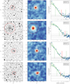 |
Fig. A.1. Same as Fig. 2, but for BER73, BER25, BER75, and BER26. |
| In the text | |
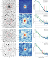 |
Fig. A.2. Same as Fig. 2, but for TOMB2, BER76, F1212, and SAU1. |
| In the text | |
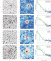 |
Fig. A.3. Same as Fig. 2, but for CZER30, ARPM2, BH4, and F1419. |
| In the text | |
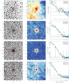 |
Fig. A.4. Same as Fig. 2, but for BH37, E9205, E9218, and SAU3. |
| In the text | |
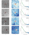 |
Fig. A.5. Same as Fig. 2, but for KRON39, E9308, BH144, and BH176. |
| In the text | |
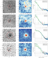 |
Fig. A.6. Same as Fig. 2, but for KRON31, SAU6, BER56, and BER102. |
| In the text | |
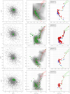 |
Fig. B.1. Same as Fig. 3, but for BER73, BER25, BER75, and BER26. |
| In the text | |
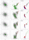 |
Fig. B.2. Same as Fig. 3, but for TOMB2, BER76, F1212, and SAU1. |
| In the text | |
 |
Fig. B.3. Same as Fig. 3, but for CZER30, ARPM2, BH4, and F1419. |
| In the text | |
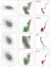 |
Fig. B.4. Same as Fig. 3, but for BH37, E9205, E9218, and SAU3. |
| In the text | |
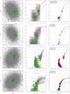 |
Fig. B.5. Same as Fig. 3 for KRON39, E9308, BH144, and BH176. |
| In the text | |
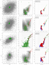 |
Fig. B.6. Same as Fig. 3, but for KRON31, SAU6, BER56, and BER102. |
| In the text | |
Current usage metrics show cumulative count of Article Views (full-text article views including HTML views, PDF and ePub downloads, according to the available data) and Abstracts Views on Vision4Press platform.
Data correspond to usage on the plateform after 2015. The current usage metrics is available 48-96 hours after online publication and is updated daily on week days.
Initial download of the metrics may take a while.