| Issue |
A&A
Volume 663, July 2022
|
|
|---|---|---|
| Article Number | A12 | |
| Number of page(s) | 19 | |
| Section | Extragalactic astronomy | |
| DOI | https://doi.org/10.1051/0004-6361/202243117 | |
| Published online | 01 July 2022 | |
The halo of M 105 and its group environment as traced by planetary nebula populations
II. Using kinematics of single stars to unveil the presence of intragroup light around the Leo I galaxies NGC 3384 and M 105⋆
1
European Southern Observatory, Alonso de Cordova 3107 Vitacura, Casilla, 19001 Santiago de Chile, Chile
e-mail: This email address is being protected from spambots. You need JavaScript enabled to view it.
2
European Southern Observatory, Karl-Schwarzschild-Str. 2, 85748 Garching, Germany
3
Max-Planck-Institut für Extraterrestrische Physik, Giessenbachstraße, 85748 Garching, Germany
4
School of Physics and Astronomy, University of Nottingham, NG7 2RD Nottingham, UK
5
Leiden Observatory, Leiden University, PO Box 9513 2300 RA Leiden, The Netherlands
6
DARK, Niels Bohr Institute, University of Copenhagen, Lyngbyvej 2, 2100 Copenhagen, Denmark
7
Inter University Centre for Astronomy and Astrophysics, Ganeshkhind, Post Bag 4, Pune 411007, India
8
Department of Physics, University of Oxford, Denys Wilkinson Building, Keble Road, Oxford OX1 3RH, UK
9
INAF – Osservatorio Astronomico di Capodimonte, Via Moiariello 16, 80131 Naples, Italy
10
Departamento de Astronomia, Instituto de Astronomia, Geofisica e Ciencias Atmosfericas da USP, Cidade Universitaria, 05508900 Sao Paulo, Brazil
11
Research School of Astronomy & Astrophysics Mount Stromlo Observatory, Cotter Road, 2611 Canberra, Australia
12
School of Physics and Astronomy, Sun Yat-sen University, DaXue Road 2, 519082 Zhuhai, PR China
13
CSST Science Center for the Guangdong-Hongkong-Macau Greater Bay Area, DaXue Road 2, 519082 Zhuhai, PR China
14
Department of Physics & Astronomy, San José State University, One Washington Square, San Jose, CA 95192, USA
15
University of California Observatories, 1156 High St., Santa Cruz, CA 95064, USA
16
Department of Astronomy and Astrophysics, University of California, Santa Cruz, CA 95064, USA
Received:
14
January
2022
Accepted:
14
February
2022
Abstract
Context. M 105 (NGC 3379) is an early-type galaxy in the nearby Leo I group, the closest galaxy group to contain all galaxy types and therefore an excellent environment to explore the low-mass end of intra-group light (IGL) assembly.
Aims. We present a new and extended kinematic survey of planetary nebulae (PNe) in M 105 and the surrounding 30′×30′ in the Leo I group with the Planetary Nebula Spectrograph (PN.S) to investigate kinematically distinct populations of PNe in the halo and the surrounding IGL.
Methods. We use PNe as kinematic tracers of the diffuse stellar light in the halo and IGL, and employ photo-kinematic Gaussian mixture models to (i) separate contributions from the companion galaxy NGC 3384, and (ii) associate PNe with structurally defined halo and IGL components around M 105.
Results. We present a catalogue of 314 PNe in the surveyed area and firmly associate 93 of these with the companion galaxy NGC 3384 and 169 with M 105. The PNe in M 105 are further associated with its halo (138) and the surrounding exponential envelope (31). We also construct smooth velocity and velocity dispersion fields and calculate projected rotation, velocity dispersion, and λR profiles for the different components. PNe associated with the halo exhibit declining velocity dispersion and rotation profiles as a function of radius, while the velocity dispersion and rotation of the exponential envelope increase notably at large radii. The rotation axes of these different components are strongly misaligned.
Conclusions. Based on the kinematic profiles, we identify three regimes with distinct kinematics that are also linked to distinct stellar population properties: (i) the rotating core at the centre of the galaxy (within 1Reff) formed in situ and is dominated by metal-rich ([M/H] ≈ 0) stars that also likely formed in situ, (ii) the halo from 1 to 7.5Reff consisting of a mixture of intermediate-metallicity and metal-rich stars ([M/H] > −1), either formed in situ or was brought in via major mergers, and (iii) the exponential envelope reaching beyond our farthest data point at 16Reff, predominately composed of metal-poor ([M/H] < −1) stars. The high velocity dispersion and moderate rotation of the latter are consistent with those measured for the dwarf satellite galaxies in the Leo I group, indicating that this exponential envelope traces the transition to the IGL.
Key words: galaxies: individual: M 105 / galaxies: elliptical and lenticular / cD / galaxies: groups: individual: Leo I / galaxies: halos / planetary nebulae: general
Full Tables A.1 and A.2 are only available at the CDS via anonymous ftp to cdsarc.u-strasbg.fr (130.79.128.5) or via http://cdsarc.u-strasbg.fr/viz-bin/cat/J/A+A/663/A12
© ESO 2022
1. Introduction
The galaxy M 105 (NGC 3379) of the Leo I group prominently featured in a lively debate over the dark matter (DM) content and its spatial distribution in massive early-type galaxies (ETGs; Romanowsky et al. 2003; Dekel et al. 2005; de Lorenzi et al. 2009; Napolitano et al. 2009; Morganti et al. 2013). Using data obtained with the Planetary Nebula Spectrograph (PN.S), Romanowsky et al. (2003) and Douglas et al. (2007) found that several intermediate-luminosity elliptical galaxies – M 105 among them – appeared to have low-mass and low-concentration DM halos, if any, based on their rapidly falling velocity dispersion profiles. This is in contrast with inferences made for the massive dark halos of giant elliptical galaxies from multiple tracers, such as the spectra of integrated light (e.g., Kronawitter et al. 2000; Gerhard et al. 2001; Cappellari et al. 2006), X-ray profiles of the hot gas atmospheres (e.g., Awaki et al. 1994; Loewenstein 1999; Humphrey et al. 2012), and weak and strong gravitational lensing (e.g., Hoekstra et al. 2004; Mandelbaum et al. 2006; Wilson et al. 2001; Koopmans et al. 2006; Tortora et al. 2010, 2014). Follow-up studies discussed whether the apparent lack of DM in the halo of M 105 was linked to the gravitational potential-orbital anisotropy degeneracy and viewing-angle effects (Dekel et al. 2005; Douglas et al. 2007; de Lorenzi et al. 2009; Weijmans et al. 2009; Morganti et al. 2013). Furthermore, the strong decrease in the line-of-sight (LOS) velocity dispersion may not continue in the outer halo; Pulsoni et al. (2018) identified several ETGs where the decline in the LOS velocity dispersion was followed by an increase in the outer halo (e.g., NGC 1023, NGC 2974, NGC 4374, NGC 4472). As the measurements of Romanowsky et al. (2003) were confined within eight effective radii (i.e. within the field of view of a single PN.S pointing and assuming an effective radius of  , Capaccioli et al. 1990), they may have missed a kinematic transition at larger radii.
Using new, extended imaging and kinematic samples of planetary nebulae (PNe), we aim to investigate whether the LOS velocity dispersion profile decline in M 105 continues in the outer halo or whether a change in kinematics is observed. Our work builds on the first paper in this series, in which Hartke et al. (2020, hereafter H+2020), presented a wide-field photometric survey of PN candidates in M 105 and the surrounding 0.5 × 0.5deg2. H+2020 found a variation of the luminosity-specific PN number α (as defined in Sect. 3.4) with radius in the halo of M 105, with the α-parameter being seven times higher in the extended halo than in the inner halo. These authors inferred that the PN population with a high α-parameter is linked to a diffuse population of metal-poor stars ([M/H] ≤ −1.0, Lee & Jang 2016), whose light distribution is governed by an exponential surface brightness (SB) profile. The light distribution in the inner halo is dominated by intermediate-metallicity and metal-rich stars ([M/H] > −1.0, Lee & Jang 2016) following a Sérsic SB profile and a low-α-parameter population of PNe. In this paper, which is the second of the series, we wish to investigate whether the two PN populations that H+2020 identified also possess distinct kinematic signatures and which constraints these would place on the assembly history of M 105 and its group environment, the Leo I group.
The Leo I group is the closest group that contains all (i.e. early and late) galaxy types (de Vaucouleurs 1975). The eleven brightest and most massive member galaxies can be further divided into two subgroups. Four are associated with the so-called Leo Triplet. The remaining seven, among them M 105 and NGC 3384, which are the main subjects of this paper, are associated with the M 96 (NGC 3368) group. In addition to these bright member galaxies, dwarf galaxies make up the largest number of group members: Müller et al. (2018) compiled the most recent catalogue of dwarf galaxies in the group, adding 36 new candidates to the previously known 52 dwarf galaxies.
With its low mass and proximity, the Leo I group is an excellent environment in which to explore the low-mass end of intra-group light (IGL) assembly. Based on deep and wide-field photometry, Watkins et al. (2014) attributed at most a few per cent of the light in their survey footprint to the IGL. Assuming that all PNe associated with the exponential SB profile trace the IGL, H+2020 determine the fraction of PNe associated with the IGL to be 22%, while the fraction in terms of stellar SB is 3.8%. This low IGL fraction seemingly contradicts results from numerical simulations, which predict IGL fractions of between 12% and 45% (Sommer-Larsen 2006; Rudick et al. 2006). However, it is unclear whether this mismatch is a resolution effect or whether a dimmer IGL is expected in lower mass groups compared to more massive environments such as galaxy clusters (Purcell et al. 2007; Watkins et al. 2014). Evaluating the dynamical status of the PNe populations at large radii is imperative for constraining the IGL properties in the Leo I group.
This paper is organised as follows: in Sect. 2, we describe the data from photometric and slitless spectroscopic surveys in the Leo I group and the compilation of the final cross-matched data catalogues. Section 3 describes the decomposition of the sample into PNe associated with NGC 3384 and M 105 based on photo-kinematic models. We describe the kinematics of PNe in the halo and envelope of M 105 in Sect. 4. We discuss our results in Sect. 5 and put them into the context of the Leo I group at large. We summarise and conclude our findings in Sect. 6.
In this paper, we adopt a physical distance of 10.23 Mpc to M 105. The corresponding physical scale is 49.6 pc/″. This tip of the red giant branch (TRGB) distance was independently determined by Harris et al. (2007a,b) and Lee & Jang (2016) and agrees well with that determined from the bright cut-off of the planetary nebula luminosity function (PNLF) determined by H+2020 as well as with that derived from SB fluctuation measurements (SBF; Tonry et al. 2001). The effective radius of M 105 derived from broad-band photometry is  (Capaccioli et al. 1990), corresponding to a physical scale of 2.7 kpc.
2. The data
2.1. Photometric survey
H+2020 presented the Subaru Surprime-Cam survey for PNe candidates in the Leo I group. Here, we only briefly summarise the survey objectives, data reduction, and PN candidate identification and validation. H+2020 identified PN candidates from the combined use of narrow- [O III] (λc,on = 5500 Å) and broad-band V-band (λc,off = 5029 Å) images. Using CMD-based automated detection techniques (Arnaboldi et al. 2002, 2003), these authors identified 226 PNe candidates within a limiting magnitude of m5007, lim = 28.1. These candidates are denoted by grey crosses in the right panel of Fig. 1. The photometric survey thus covers 2.6 magnitudes from the bright cut-off of the PNLF at  . The unmasked survey area (excluding image artefacts and regions with a high background value) covered 0.2365 deg2 on the sky, which corresponds to 67.7 kpc along the major axis of M 105. The survey also covers the halos of NGC 3384 and NGC 3389. The survey footprint is outlined by the grey dashed rectangle in the left panel of Fig. 1. The IDs, coordinates, and magnitudes of the PNe candidates brighter than the limiting magnitude are presented in Table A.1.
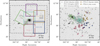 |
Fig. 1. DSS image of the Leo I group with a scale-bar in the lower-right corner indicating a physical scale of 10 kpc. North is up, east to the left. Left: rectangles show the field outlines of the Surprime-Cam photometry survey (grey dashed outline), individual fields of the e2PN.S survey (solid outlines), and the HST fields analysed by Lee & Jang (2016, hashed rectangles). Right: overplotted are the PN candidates detected with Surprime-Cam (Hartke et al. 2020, grey plus symbols). The data from the ePN.S survey (Pulsoni et al. 2018) for NGC 3384 (first published by Cortesi et al. 2013a) and M 105 (first published by Douglas et al. 2007) are indicated by cyan and green points and diamonds respectively. Squares denote the PNe from the e2PN.S survey already presented in (H+2020) and bold crosses newly detected PNe from this work. The colours of the symbols correspond to those of the field outlines in the left panel. |
2.2. The extremely extended PN.S ETG survey in M 105 and NGC 3384
The extremely extended PN.S ETG (e2PN.S) survey includes data from the ePN.S survey (Arnaboldi et al. 2017; Pulsoni et al. 2018), namely two fields centred on M 105 and NGC 3384 respectively. The first PN.S observations of M 105 were part of the PN.S ETG survey (Douglas et al. 2007). The resulting 214 PNe are indicated with cyan circles in the right panel of Fig. 1 and in the left panel, where the field is outlined in the same colour and denoted M 105-C.
In 2017, we observed two additional fields (M 105-W and M 105-S). These are indicated by the brown and red rectangles in the left panel of Fig. 1. These data were used to independently validate the photometric sample in H+2020. In 2019, M 105-W was observed again, along with the fields M 105-SW (blue rectangle) and M 105-N (purple rectangle). The total exposure times per field are given in Table 1. NGC 3384 was first observed as part of the PN.S survey of S0 galaxy kinematics (Cortesi et al. 2013a). In total, 101 PNe were observed; these are shown with green diamonds in the right panel of Fig. 1. The availability of these data will enable an improved photo-kinematic decomposition of the PN sample (see Sect. 3).
Summary of the PN.S observations used in this paper.
2.2.1. Field-to-field variation and catalogue matching within the e2PN.S survey
The PN.S pipeline processes the survey data field by field. We therefore had to cross-match the individual catalogues to create a homogeneous master catalogue encompassing data from the six fields. We used an iterative coordinate-matching algorithm with a matching radius of 5″. We chose this seemingly large radius due to the positional uncertainties on the PN.S data. As already stated in H+2020, we identify the 30 PNe with measurements in the fields M 105-C and N3384. In addition to that, we identify 2 PNe in M 105-S and M 105-SW, 1 PN in M 105-N and M 105-W, and 6 in M 105-C and M 105-W.
Figure 2 shows a field-to-field comparison of the velocities. The velocity measurements generally scatter about the one-to-one line, and the scatter is within the 2σ PN.S velocity error (light grey shaded region). H+2020 already discussed the nature of the 11 measurements that lie outside of the grey shaded region: these 11 PNe were observed close to one of the field edges in either of the two fields. For these objects, only the measurements taken closer to the respective field centre were included in the final catalogue. For the other PNe with repeat measurements, we included the mean velocities and magnitudes instead. The IDs of PNe with repeated measurements were concatenated in the final catalogue.
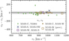 |
Fig. 2. Comparison of the velocity measurements obtained for PNe that lie in the areas of intersection of the two fields. The grey shaded regions indicate the nominal 1σ and 2σ PN.S velocity uncertainties of ±20 and ±40 km s−1, respectively. For the M 105-W field, ‘prev.’ indicates the previous measurements by H+2020. |
We also identified 5 PNe in the western field based on 2017 data alone (H+2020) and in the deeper stack, including the data from 2019. These are denoted with orange squares in Fig. 2. They all scatter about the one-to-one line, and the scatter is within the velocity error of the PN.S. We conclude that there is no velocity offset between the observations taken in 2017 and 2019.
2.2.2. Photometric calibration and catalogue matching with Surprime-Cam photometry
We matched the kinematic catalogue compiled in the previous section with the photometric one from H+2020. Like H+2020, we used a matching radius of 5″ due to the relatively large positional uncertainty on the PN.S data. We used this matched sample to determine the zero-point magnitude of each of the newly observed PN.S fields. Figure 3 shows a comparison of the AB magnitudes obtained with the PN.S after applying the zero-point offset with those from Surprime-Cam. The colour-coding is the same as in Fig. 1.
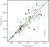 |
Fig. 3. Comparison of the AB magnitudes of PN candidates from H+2020 with those from the e2PN.S survey. The colour coding is the same as in the left panel of Fig. 1. The grey shaded region indicates where 99% of Subaru sources would fall if one plotted two independent measurements of their magnitudes mAB, Subaru against each other H+2020. The error bar in the lower right corner denotes the typical magnitude uncertainty of the PN.S. |
The large scatter about the one-to-one line is not surprising, as the PN.S had not been optimised to obtain accurate photometry. While the photometric accuracy is acceptable in nearby galaxies (e.g., Merrett et al. 2006), Hartke et al. (2018) found a similarly large scatter of PN.S magnitudes compared to accurate Surprime-Cam ones in the Virgo galaxy M49. In order to convert the AB magnitudes to m5007, we used the relation determined by Arnaboldi et al. (2003): m5007 = mAB + 2.49.
To gauge the depth of the e2PN.S survey, we constructed the PNLF of each of the fields. Figure 4 shows the PNLF for each field with the same colour coding as in Fig. 1. The black histogram denotes the PNLF of all e2PN.S PNe. For comparison, we also show the PNLF based on the Surprime-Cam photometry in grey. We only included data brighter than the limiting magnitude m5007, lim = 28.1. The vertical dotted lines denote the PNLF bright cut-offs corresponding to the distances to M 105 (black,  ) and NGC 3384 (grey,
  ) respectively. Except for one over-luminous object, all PNe are fainter than the bright cut-off
  .
.
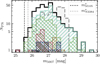 |
Fig. 4. PNLF of all PNe from the e2PN.S survey (black histogram) and its individual fields. The colour-coding of the histograms corresponds to that in Fig. 1. The dashed grey histogram denotes the PNLF from the Surprime-Cam photometry. No completeness corrections have been applied to any of the LFs. The black and grey dotted vertical lines denote the PNLF bright cut-offs corresponding to the distance of M 105 and NGC 3384, respectively. |
The deepest fields are centred on M 105 and NGC 3384, with the faintest object nearly reaching 30th magnitude. However, the e2PN.S survey is likely only complete to a limiting magnitude of m5007, lim = 27.5. This is the magnitude at which the number of PNe starts to decrease as a function of magnitude, contrary to the exponential increase that is theoretically expected (see also H+2020).
2.2.3. Excluding velocity outliers
To remove velocity outliers that may be sources of contamination, we first calculated the mean velocity and velocity dispersion σ of the whole sample – including PNe associated with M 105 and NGC 3384 – using a robust fitting technique (McNeil et al. 2010). The left panel of Fig. 5 shows the phase-space of PN candidates in the e2PN.S footprint with the x-coordinate along the major axis of M 105. The right panel of Fig. 5 shows the corresponding LOS velocity distribution (LOSVD) with the 1, 2, and 3σ intervals shaded in blue. The velocity range covered by the different filter configurations is −400 < v ≤ 2400 km s−1. We clipped four PNe with velocities outside the velocity range of ±3σ about the robust mean. Table 1 contains the final e2PN.S catalogue after combining observations from multiple fields, correcting the magnitude zero-point, and 3σ-clipping. In summary, the final catalogue provided in Table A.2 contains coordinates, velocities, and magnitudes for 319 PNe.
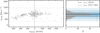 |
Fig. 5. Left: phase-space of PN candidates in the e2PN.S survey footprint, including PNe associated with M 105 and NGC 3384. The major axis of M 105 is denoted with xM 105. Right: line-of-sight velocity histogram of the objects shown in the left panel. The dashed line denotes the systemic velocity of M 105, and the solid blue line the mean velocity of the sample. The blue shaded regions denote the 1, 2, and 3σ intervals from the mean. Objects beyond 3σ of the mean velocity are likely redshifted background emission-line galaxies. |
2.2.4. Completeness and sources of contamination
The completeness of the photometric catalogue was extensively discussed in H+2020. Due to the nature of the PN.S instrument, we can immediately discard objects with a continuum, as the continuum appears as a stripe in slitless spectroscopy. This requirement excludes the majority of Ly-α emitters with a continuum redder than the [O III]5007 Å emission line. Background [O II] emitters at z ≃ 0.34 can be discarded as the spectral resolution of the PN.S is sufficient to resolve both emissions from the redshifted [O II] 3727 Å doublet. However, we cannot use the second bluer line of the [O III] doublet commonly used to distinguish PNe from contaminants as it is not covered by the PN.S bandpass. We therefore resorted to statistical methods to estimate the contamination from Ly-α galaxies without a measurable continuum, assuming that the number of background galaxies is uniformly distributed in a velocity histogram (Spiniello et al. 2018).
Based on the presence of three objects in the velocity range 1400 < v ≤ 2400 km s−1 and one in the velocity range −400 < v ≤ 400 km s−1 (see Fig. 5), which are likely not PNe, we expect 7 objects such as background galaxies in the full velocity range, corresponding to a fraction of 2.2%. The result is very similar to that estimated by H+2020 (2.6%) based on a subset of the data and the estimate of Spiniello et al. (2018, ≈2%) for slitless spectroscopy of PNe in the Fornax cluster.
3. Galaxy membership assignment based on photo-kinematic models
In order to decompose the kinematic PN sample into subcomponents associated with M 105 and NGC 3384, we modelled the observed PN in position–velocity space using a luminosity-weighted multi-Gaussian model. The luminosity weights are pre-determined from broad-band photometry, while the kinematic parameters are free parameters of the Gaussian-mixture model. Gaussian-mixture models are widespread in the astronomical literature to disentangle multi-component LOSVDs (see e.g., Walker & Peñarrubia 2011; Amorisco & Evans 2012; Watkins et al. 2013; Agnello et al. 2014; Hartke et al. 2018; Longobardi et al. 2018a). In the following simple modelling, we assume that there is no strong ongoing interaction between the two galaxies. This assumption is supported by the absence of strong tidal features or bridges of stars connecting the two galaxies (Watkins et al. 2014).
3.1. Disk–bulge decomposition of NGC 3384
To model the kinematics of NGC 3384, we use the disk-bulge decomposition method developed by Cortesi et al. (2011) and subsequently applied to the PN.S survey of S0 galaxy kinematics (Cortesi et al. 2013b), including the decomposition of NGC 3384 into its disk and bulge components.
The LOS velocity of the disk as function of azimuthal angle ϕ3384 and radius r3384 measured with respect to the centre of NGC 3384 can be expressed as
 (1)
(1)
where vrot is the mean rotation velocity of the galaxy and i the inclination at which the disk is observed. The corresponding velocity dispersion is
 (2)
(2)
where σr, σϕ, and σz are its components in cylindrical coordinates. In edge-on galaxies, the contribution along the z-axis is small. Hence, in the following the term  can be dropped. Assuming a Gaussian LOSVD, the disk kinematics can be described as
 (3)
(3)
The contribution from the bulge is described as a Gaussian centred on the systemic velocity of NGC 3384 with velocity dispersion σN3384, bulge, assuming it does not rotate significantly:
 (4)
(4)
The two kinematic components of the LOSVD are weighted by the SB profiles as described in Sect. 3.3. In order to account for the variation of the LOSVD as a function of radius, we evaluate it in five concentric elliptical bins with the same geometry as the galaxy’s isophotes centred on NGC 3384. Therefore, the parameters vrot, σr, σϕ, and σN3384, bulge are evaluated independently in each of the five bins. Following Cortesi et al. (2011, 2013b), we can reduce the parameter space using the epicycle approximation that holds for disk galaxies with approximately flat rotation curves (see, e.g., Binney & Tremaine 1987) and links the radial velocity dispersion with the tangential one:  .
.
3.2. Kinematic model of M 105
Following the discovery of a PN population associated with an exponential SB profile in addition to the Sérsic halo (H+2020), we model M 105’s kinematics LOSVD with two Gaussians; both centred on the galaxy’s systemic velocity vsys, M 105. They differ in their velocity dispersions, which we denote with σM 105, Ser and σM 105, Exp, respectively:
 (5)
(5)
 (6)
(6)
Again, in order to account for any variation of the LOSVD with radius, the parameters σM 105, Ser and σM 105, Exp are evaluated in five concentric elliptical annuli with the same geometry as the galaxy’s isophotes, but this time centred on M 105. We assume that the LOS velocity dispersion of the exponentially distributed PN population is larger than that of the one following a Sérsic profile in each bin.
3.3. Constraints on galaxy membership from broad-band photometry and RGB star number counts
As the number density distribution of PNe is closely linked to the stellar light distribution, i.e. the galaxies’ SB profiles (see e.g., Coccato et al. 2009, and Fig. 7), we can obtain further constraints on which PN belongs to which galaxy component from broad-band photometry. The SB profiles of M 105 and NGC 3384 are described by a combination of Sérsic profiles (Sérsic 1963). The intensity I as a function of radius R is:
![Mathematical equation: $$ \begin{aligned} I_{\mathrm{Ser}} (R) = I_{\mathrm{eff}} \exp \left( -b_n \left[\left(\frac{R}{R_{\mathrm{eff}} }\right)^{1/n} -1\right]\right), \end{aligned} $$](/articles/aa/full_html/2022/07/aa43117-22/aa43117-22-eq15.gif) (7)
(7)
with
 (8)
(8)
The effective intensity Ieff is measured at the effective radius Reff at which half the luminosity is enclosed, and the steepness of the profile is controlled by the Sérsic index n. The corresponding SB profile is
![Mathematical equation: $$ \begin{aligned} \mu _{\mathrm{Ser}} (R) = \mu _{\mathrm{eff}} + \frac{2.5 b_n}{\ln 10}\left[\left(\frac{R}{R_{\mathrm{eff}} }\right)^{1/n} -1\right], \end{aligned} $$](/articles/aa/full_html/2022/07/aa43117-22/aa43117-22-eq17.gif) (9)
(9)
with the effective SB μeff = −2.5 log Ieff.
An exponential SB profile with scale length h is a special case of the Sérsic profile with index n = 1:
 (10)
(10)
The scale length h and central SB μ0 are related to the Sérsic quantities as follows:
 (11)
(11)
In the following, we describe the structural parameters of NGC 3384 and M 105 that were derived in previous works. Table 2 provides a summary in terms of Sérsic structural parameters, and Fig. 6 shows the resulting SB maps for the two galaxies separately, as well as a composite SB map.
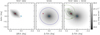 |
Fig. 6. Modelled SB maps of NGC 3384 (left) and M 105 (centre), with the centres of the galaxies marked with red and blue crosses, respectively. Right panel: composite SB map from both galaxies and green contours where M 105 contributes 90%, 50%, and 10% of the total light distribution. |
Structural parameters of M 105 and NGC 3384 derived from broad-band surface photometry (Watkins et al. 2014; Cortesi et al. 2013b; Skrutskie et al. 2006) and PN number counts (H+2020) used as input for the photo-kinematic decomposition.
3.3.1. NGC 3384
Cortesi et al. (2013b) analysed 2MASS K-band images (Skrutskie et al. 2006) with GALFIT (Peng et al. 2010) for the disk–bulge decomposition of NGC 3384. These authors found that the light distribution of the bulge in the K-band is best described by a Sérsic profile with effective SB μeff, bulge = 15.9, Sérsic index n = 4, effective radius  , ellipticity ϵbulge = 0.17, and position angle
  .
.
The light distribution of the disk is described with an exponential profile with central SBs μ0, disk = 18.25, scale length  , ellipticity ϵN3384, disk = 0.66, inclination i = 70°, and
  . H+2020 determined a colour correction of B − K = −3.75 for the profiles derived from the 2MASS data by Cortesi et al. (2013b). The left panel of Fig. 7 shows the total B-band SB profile of NGC 3384 (grey line) and the contributions from the galaxy disk (blue dashed line) and bulge (red dotted line).
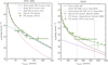 |
Fig. 7. Stellar SB profiles of NGC 3384 and M 105 in comparison with PN number density profiles scaled by the respective α-parameters. In both panels, the solid grey line denotes the total stellar SB, and the dark green error bars show the PN number density based on data from the PN.S. Left: stellar SB profile of NGC 3384 decomposed into bulge (dotted red line) and disk (dashed blue line) by Cortesi et al. (2013b) and the best-fit PN number density profile is denoted by the dash-dotted green line. Right: stellar SB profile of M 105 decomposed into Sérsic (dotted orange line) and exponential (dashed purple line) components by H+2020 with priors on the number-densities of metal-poor and metal-rich RGB stars from Lee & Jang (2016) and fit to the PN number density from Surprime-Cam data alone (light green error bars). The grey dotted vertical line denotes the radius at which the PN number density starts to deviate from the stellar SB profile and the dashed vertical line where the exponential SB starts to dominate the total light distribution. |
3.3.2. M 105
The light distribution of M 105 was first analytically described by de Vaucouleurs (1948), and is still regarded as one of the cornerstones of the de Vaucouleurs law today. Combining number density profiles of resolved red giant branch (RGB) stellar populations (Lee & Jang 2016) with deep wide-field imaging (Watkins et al. 2014), and their wide-field photometric survey for PNe, H+2020 established a two-component model for the SB profile of M 105. The light distribution in the inner halo is dominated by metal-rich stars following a Sérsic profile with nSer = 2.75, Reff, Ser = 57″, and μeff, Ser = 21.73, denoted by the dotted orange line in the right panel of Fig. 7. The fractional contribution from metal-poor stars increases in the outer halo. Their light distribution is modelled with an exponential profile with hExp = 358″ and μ0, Exp = 27.7. Watkins et al. (2014) derived a constant ellipticity of ϵM 105 = 0.111 ± 0.005 and a position angle of  in the outer halo of M 105.
3.4. PN-specific frequency dependency on stellar population parameters
As the number of PNe has been shown to systematically vary with the colour of the parent stellar population (Buzzoni et al. 2006; Longobardi et al. 2015; Hartke et al. 2017), such dependency must be taken into account when using SB profiles derived from integrated starlight as weights for the kinematic model. The connection between a PN population and the underlying stellar population is given by the luminosity-specific PN number, referred to here as the α-parameter, which relates the total number of PNe NPN to the total bolometric luminosity Lbol of the parent stellar population:
 (12)
(12)
For the bolometric correction, we use that derived from theoretical template galaxy models as a function of galaxy colour (Buzzoni 2005; Buzzoni et al. 2006). In the following, we refer to α2.5 values, which are calculated in the magnitude interval m* < m5007 ≤ m* + 2.5. The observed PN number densities for NGC 3384 and M 105 are indicated with green error bars in the left and right panels of Fig. 7, respectively.
For NGC 3384, we assume that the α-parameters for disk and bulge are equal (because incompleteness in the centre of the galaxy means we cannot calculate αbulge separately) and determined  . We only considered PNe that lie within the green 50% contour shown in the right panel of Fig. 6. The resulting best-fit PN number density profile is indicated by the green dash-dotted line in the left panel of Fig. 7.
For M 105, H+2020 determined α-parameters for PNe associated with the Sérsic and exponential SB profiles and found  and
and  . The resulting best-fit PN number density profile is indicated by the green dash-dotted line in the right panel of Fig. 7. As the bulk of the light in M 105 is contributed by metal-rich stars following the Sérsic profile, we use αM 105, Ser as the denominator of the normalisation. We therefore include the parameters
  and
and  which characterise the variation of α in the bulge and disk components of NGC 3384, as well as in the outer halo of M 105 with respect to the α-parameter of the main halo of M 105.
3.5. Bayesian likelihood
The likelihood of a PN k with observed position RA, Dec and velocity vk ± δvk can be expressed in terms of the velocity and surface-brightness distributions that we define in the previous three sections. The model component weights are defined as follows:
 (13a)
(13a)
 (13b)
(13b)
 (13c)
(13c)
 (13d)
(13d)
where both the α-parameters and the surface-brightness profiles Σ are completely determined by the broad- and narrow-band photometry as described in Sects. 3.3 and 3.4. The weights are normalised by
 (14)
(14)
The corresponding likelihood for a PN k at its position in phase-space is
 (15)
(15)
The total likelihood is the product of the individual likelihoods calculated for each individual PN with coordinates (RA, Dec) and LOS velocity v ± δv:
 (16)
(16)
This method allows us to exploit the information available for every PN without the explicit need for binning in velocity space. As discussed in Sects. 3.1 and 3.2, we evaluate the five LOSVD parameters vrot, σr, σN3384, bulge, σM 105, Ser, and σM 105, Exp independently in five elliptical annuli centred on the respective galaxies (solid and dashed ellipses in Fig. 9). This results in a parameter space of 25 dimensions, which is explored using the ensemble-based MCMC sampler EMCEE (Foreman-Mackey et al. 2013).
3.6. Priors and posteriors
As Cortesi et al. (2013b) already carried out a bulge–disk decomposition of NGC 3384 based on the single PN.S field available to them at the time, we use their best-fit parameters and corresponding errors as Gaussian priors on vrot, σr, σϕ, σN3384, bulge. As we evaluate the LOSVD in five elliptical bins instead of three, we interpolated their best-fit profiles as a function of radius and used the interpolated values at the bin centres. An example of the Gaussian priors for the innermost of the five elliptical bins is indicated with red solid lines in Fig. 8. We place uniform priors on σM 105, Ser and σM 105, Exp, but require σM 105, Ser ≤ σM 105, Exp in each of the bins.
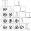 |
Fig. 8. Posterior probability distribution of the parameters σsph (the velocity dispersion of the bulge of NGC 3384), σr, and vrot (the radial velocity dispersion and circular velocity of the disk of NGC 3384), and σM 105, Ser and σM 105, Exp (the velocity dispersions of the Sérsic and exponential populations in M 105) in the innermost of the five elliptical bins. To illustrate the Gaussian priors on the LOSVD parameters of NGC 3384, which cover a larger range in parameter space, we inserted three additional subplots showing the priors with red solid lines and the posteriors with black histograms, utilising the same binning as the corner plots. The red shaded regions below the Gaussians denote 1σ from the mean. On all plots, the velocities or velocity dispersions are in units of [km s−1]. |
The posterior probability distributions are calculated with EMCEE (Foreman-Mackey et al. 2013) using 52 walkers (2Ndim + 2) and 2000 steps. Figure 8 shows the resulting distributions visualised as a corner plot for the innermost of the five elliptical bins. This is a convenient representation of a subset of the parameter space. However, we stress that the 25-dimensional space is explored simultaneously for data over the entire radial range. The best-fit parameters and their errors are the 50% and (16%, 84%) quantiles. While the best-fit parameters give a good first estimate of the LOS velocity dispersion of the Sérsic and exponential PN populations in the halo of M 105, we calculate more accurate radial velocity dispersion profiles with robust methods and based on the final membership assignment presented in the following.
3.7. Final membership assignment
For each PN, we determine the probabilistic fraction fi to belong to one of the four populations (the disk and bulge of NGC 3384, and the Sérsic and exponential halos of M 105) based on its position and LOS velocity. Figure 9a illustrates the probability space populated by our observations, with fM 105, Ser > 0.5 coloured in orange (138 PNe), fM 105, Exp > 0.5 coloured in purple (31 PNe), and fNGC 3384 > 0.5 being represented by crosses on a red-to-blue colour scale with red colours for fNGC 3384, bulge > 0.5 (37 PNe) and blue colours for fNGC 3384, disk > 0.5 (56 PNe). Points that cannot be uniquely associated with any of the four components outlined previously are colour-coded in grey (7 PNe). Figure 9b shows the distribution of PNe colour-coded by fi in position-space, and Fig. 9c,d in phase-space along the major and minor axes of M 105, respectively.
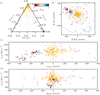 |
Fig. 9. Panel a: ternary plot of the probabilistic fractions fi with fM 105, Ser > 0.5 coloured in orange, fM 105, Exp > 0.5 coloured in purple, and fNGC 3384 > 0.5 represented by crosses on a red-to-blue colour scale with red colours for fNGC 3384, bulge > 0.5 and blue colours for fNGC 3384, disk > 0.5. Points coloured in grey do not satisfy any of the four criteria, and their association with any of the components cannot be conclusively ascertained. Panel b: spatial distribution of PNe with the same colour coding as in panel a. Panel c: velocity phase-space along the major axis of M 105 with the same colour coding as in panel a. Panel d: velocity phase-space along the minor axis of M 105 with the same colour coding as in panel a. |
Both in position- and phase-space, PNe can be robustly separated into those associated with M 105 and those with NGC 3384. This is important for the study of the LOSVD of M 105, which is presented in the following sections. We maximised the number of PNe to be considered for follow-up analysis compared to conventional cuts in position space (as e.g., done by Douglas et al. 2007), while ensuring that the derived LOSVDs are of sufficient quality. The final column of Table A.2 provides the probabilistic fraction to be assigned to M 105 fM 105 = fM 105, Ser + fM 105, Exp for each PN in the final sample. This can be easily translated to the probabilistic fraction to be assigned to NGC 3384 fNGC 3384 = 1 − fM 105.
4. Kinematics in the outer halo of M 105
In the following section, we only consider PNe that we assigned to the M 105 halo and envelope in the previous section. For the calculation of the smoothed 2D velocity and velocity dispersion fields and the extraction of the rotation profiles, we assume that M 105 is point-symmetric in the position-velocity phase-space, as commonly done when constructing velocity fields based on PN kinematics (e.g., Arnaboldi et al. 1998; Coccato et al. 2009; Pulsoni et al. 2018). This implies that each point (x, y, v) in this phase-space has a ‘mirror point’ ( − x, −y, −v) and that the number of data points with which the kinematic quantities are calculated is doubled. The resulting catalogue, that is, the concatenation of the original and mirrored catalogues, is called the folded catalogue.
4.1. Smoothed 2D velocity and velocity dispersion fields
We calculate kernel-smoothed velocity and velocity dispersion fields for all PNe associated with M 105 and for the Sérsic and exponential components separately from the folded catalogues. We use a distance-dependent Gaussian kernel as defined in Coccato et al. (2009)
 (17)
(17)
where the kernel width k(x, y) is proportional to the distance Ri, M to the Mth closest tracers located at (xM, yM):
 (18)
(18)
We use the optimised kernel parameters A = 0.34 and B = 16.2 for the M = 20 closest tracers, which were determined by Pulsoni et al. (2018) based on Monte Carlo simulations of discrete velocity fields, allowing for the best compromise between noise smoothing and spatial resolution.
Figure 10 shows the resulting smoothed velocity vs (top row) and velocity dispersion σs fields (bottom row) for all PNe associated with M 105 in the left column, and the Sérsic and exponential components shown in the middle and right columns, respectively. The smoothed velocity and velocity dispersion fields of the Sérsic and exponential components show distinct features. As expected from the method with which PNe were associated to either component, the LOS velocity dispersion of PNe in the exponential component is much larger than that of those in the Sérsic one, even at comparable radial ranges. The rotation signatures in the velocities are also different, suggesting that different mechanisms contributed to the formation of the Sérsic and exponential components in the halo of M 105.
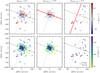 |
Fig. 10. Kernel-smoothed velocity (top row) and velocity dispersion fields (bottom row) for PNe associated with M 105 in general (left column), the Sérsic component (middle column), and the exponential component (left column). Each point denotes the position of an observed PN, and is colour coded according to the value of the smoothed field. The solid (dotted) grey lines denote the photometric major (minor) axis and the dashed red line shows the kinematic major axis. North is up, and east is to the left. |
4.2. Line-of-sight velocity dispersion profiles
To determine the LOS velocity dispersion profiles, we again only consider PNe with fM 105 = fM 105, Ser + fM 105, Exp > 0.5, that is, PNe firmly associated with M 105 and the exponential envelope both in position and velocity space. We already obtained velocity dispersions in the five elliptical bins from the likelihood analysis presented in Sect. 3.7 for the Sérsic and exponential components separately. However, to explore a finer resolution along the radial direction and be more robust to potential outliers, we re-bin the data and use robust estimation methods (McNeil et al. 2010) with a clipping range of 2σ.
Figure 11 shows the resulting LOS velocity dispersion for all PNe associated with M 105 and the corresponding uncertainty. The overall velocity dispersion agrees well with that presented in de Lorenzi et al. (2009) where the data overlaps, as well as with long-slit data in the innermost region of the galaxy from Statler & Smecker-Hane (1999) and Kronawitter et al. (2000) as well as with SAURON integral-field spectroscopic data (Weijmans et al. 2009).
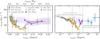 |
Fig. 11. Left: LOS velocity dispersion profiles of M 105 calculated with robust techniques for the total sample of PNe associated with M 105 (solid lines with grey dots), its Sérsic component (solid lines with orange squares), and the exponential envelope (solid lines with purple diamonds). The transparent bands denote the errors on the derived LOS velocity dispersions estimated with robust methods. For comparison, we also show the LOS velocity dispersion used by de Lorenzi et al. (2009, black error bars) from the M 105-C field, and the ones derived from long-slit spectroscopy (Kronawitter et al. (2000, filled black circles with error bars), Statler & Smecker-Hane (1999, open black circles with error bars)) and integral-field spectroscopy (Weijmans et al. 2009, filled grey squares with error bars), as well as the GC velocity dispersion from (Bergond et al. 2006, shown with green triangles with error bars). Right: as in the left panel, but with a logarithmic scale for the major-axis radius. The blue error bars denote the velocity dispersion calculated from the LOS velocities of satellites in the Leo I group (compiled by Müller et al. 2018). In both panels, shaded regions indicate the robust errors. The dotted grey lines denote the radius at which the α-parameter changes, and the grey dashed vertical lines where the exponential SB starts to dominate the total light distribution. The dotted red vertical line denotes the kinematic transition radius determined by Pulsoni et al. (2018). |
The velocity dispersion increases strongly beyond 400″ (corresponding to ≈7.5Reff), which also corresponds to the radius at which the PN number density starts to flatten due to a higher α-parameter value at large radii, as indicated by the dotted vertical line. The rise in the LOS velocity at large radii is thus driven by PNe associated with the exponential envelope (indicated by purple triangles on Fig. 11). These PNe have a larger LOS velocity dispersion than those associated with the Sérsic halo (orange squares). The strong decline of the LOS velocity dispersion in the inner halo is instead driven by PNe associated with the latter component.
4.3. Rotation
We first assess the different rotation signatures by separately fitting rotation curves to the smoothed velocities vs for the Sérsic and exponential populations separately as a function of position angle Θ as shown in Fig. 12, excluding the 2σ outliers identified in the previous Sect. 4.2 from further analysis. Following Pulsoni et al. (2018), we fit the mean velocity fields with the following function:
 (19)
(19)
 |
Fig. 12. Radially integrated rotation profiles of PNe associated with the Sérsic (top panel) and exponential (middle panel) populations from the kernel-smoothed velocity maps (dots with error bars). The bottom panel shows unsmoothed LOS velocities of satellite galaxies in the Leo I group colour-coded by their on-sky distance to the centre of M 105 (compiled by Müller et al. 2018). In each panel, the best-fit rotation profiles are denoted with solid grey curves, and the corresponding best-fit kinematic position angles (with respect to the photometric one) and systemic velocities are denoted with dashed and dotted grey lines. Open symbols denote PNe excluded from the fit as they lie outside of the 2σ limits determined in Sect. 4.2. |
where vsys is the systemic velocity, vrot the amplitude of the rotation, and Θ0 the kinematic position angle with respect to the photometric position angle. These parameters describe the rotation around the kinematic major axis, while s3 and a3 are the amplitudes of the third-order terms1.
Figure 12 shows the smoothed velocity as a function of the position angle Θ for the observed PNe in each of the two components. We fit rotation profiles to these data, only considering the azimuthal dependence of Eq. (19). We evaluate whether the goodness of the fit is improved by including the higher order terms with amplitudes a3 and s3 using the Bayesian information criterion (BIC). Table 3 summarises the best-fit parameters fit to the velocity fields, and the resulting best-fit rotation curves are shown in Fig. 12. Models including higher moments are preferred for both components. In the case of the Sérsic component, the fit with higher moments has both lower BIC and reduced χ2 values. For the exponential envelope, the BIC values are indistinguishable, but the fit with higher moments has a lower reduced χ2 value.
Best-fit parameters for the rotation models fit to the Sérsic and exponential velocity fields.
The Sérsic component has a rotation amplitude of vrot, Ser = 16.0 ± 1.8 km s−1 and a kinematic major axis that is aligned with the photometric major axis within the errors. This component also has a systemic velocity of vsys, Ser = 935.1 ± 1.4 km s−1 that agrees with that determined by Pulsoni et al. (2018) based on the central field of M 105. In contrast to this, the rotation amplitude of the PNe in the exponential envelope is more than three times higher, being vrot, Exp = 49.2 ± 6.7 km s−1, and the kinematic major axis is aligned with the photometric minor axis of M 105, while their systemic velocity of vsys, Exp = 934.2 ± 9.9 km s−1 agrees with that of the Sérsic component within the errors. To visualise the on-sky orientation of the photometric and kinematic major axes, they are overplotted on top of the smoothed velocity fields in Fig. 10.
To evaluate the radial dependence of the rotation profile, we again fitted Eq. (19) to the data, but in elliptical bins, for all PNe associated with M 105. We also fitted Eq. (16) to the Sérsic and exponential populations separately. Because of the smaller number of tracers per bin, we did not fit the third-order modes, as this led to noisier fits. The resulting best-fit profiles of the rotation amplitude vrot, systemic velocity vsys, and kinematic position angle Θ0 are shown in Fig. 13 from top to bottom. As already observed by Pulsoni et al. (2018), the rotation amplitude decreases in the inner halo with hints for growing rotation in the outskirts. This decrease was also inferred from long-slit spectroscopy (Statler & Smecker-Hane 1999). Our new extended data reveal that there is a transition region where the rotation amplitude remains small, followed by a strong increase of the rotation amplitude in the exponential envelope which is driven by the PNe associated with this component (purple diamonds).
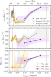 |
Fig. 13. Top: rotation amplitude along the major axis of M 105 for all PNe associated with the galaxy (grey circles), and the Sérsic (orange squares) and exponential (purple diamonds) components. The black circles with associated error bars denote the rotation profile derived from long-slit spectroscopy (Kronawitter et al. (2000, filled symbols), (Statler & Smecker-Hane 1999, open symbols)) and the grey squares that from integral-field spectroscopy (Weijmans et al. 2009). Middle: systemic velocity as a function of major-axis radius with the same colour coding as in the top panel. Bottom: best-fit kinematic position angle with respect to the photometric one as a function of major-axis radius with the same colour coding as in the top panel. In both panels, shaded regions indicate the standard errors from the maximum-likelihood fit and the vertical lines are the same as in Fig. 11. |
This transition goes hand in hand with a twisting of the kinematic position angle that is illustrated in the bottom panel of Fig. 13. In the inner halo, where the Sérsic population dominates, the kinematic position angle is aligned with the photometric one. In contrast, in the outer halo, the position angle twists by more than 90° and is more or less aligned with the photometric minor axis of the inner high SB regions.
4.4. Angular-momentum content
Emsellem et al. (2007) introduced a kinematic classification scheme for galaxies based on the so-called λR parameter, which quantifies rotational support and can be used as a proxy to quantify the observed projected stellar angular momentum. To infer the angular momentum content locally, i.e. in elliptical bins with mean radius Rmean and bin edges Rmin and Rmax, λR can be calculated from the smoothed velocity and velocity dispersion fields V and σ:
 (20)
(20)
The cumulative λR profiles are instead calculated from the centre of the galaxy to the outer bin edge Rmax and corrected for geometric incompleteness cgeo:
 (21)
(21)
The cumulative λR is weighted by the flux associated with each radial bin. For PNe, this is implicitly incorporated as the PN number density traces the light distribution (Coccato et al. 2009). When ordered motion dominates (i.e. rotation), λR approaches unity. Within one effective radius, λR can be used as a proxy to divide galaxies into the categories of fast (λR > 0.1) and slow rotators (λR < 0.1). M 105 has been classified as a fast rotator (Emsellem et al. 2007; Coccato et al. 2009; Pulsoni et al. 2018).
The left panel of Fig. 14 shows the local λR profiles for all PNe associated with M 105, the Sérsic halo, and the exponential envelope, evaluated in the same elliptical annuli as used in Figs. 13 and 11. In the inner halo, the kinematic transition radius identified by Pulsoni et al. (2018) is marked by a decrease in the local λR profile, which persists until ∼2Reff. At ∼4Reff, the λR profile peaks again. At large radii, that is, in the exponential envelope, λR increases, reaching values of λR = 0.4 in the outermost bin. The right panel of Fig. 14 shows the cumulative λR profiles. Based on the two panels, we identify three distinct kinematic components, which are discussed further in the following section: the rotating core within 1Reff, the halo from 1Reff to 7.5Reff, and the exponential envelope from 7.5Reff to the last data point at 16Reff.
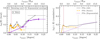 |
Fig. 14. Left: local λR profiles calculated for the total sample of PNe associated with M 105 (grey), its Sérsic component (orange), and the exponential envelope (purple). Horizontal error bars denote the bins in which λR was evaluated. Right: cumulative λR profiles, with the same colour coding as in the left panel. In both panels, the dotted grey line at λR = 0.1 separates fast from slow rotator regions assuming constant ellipticity (Emsellem et al. 2007). The vertical dotted lines are the same as in Fig. 11. |
5. Discussion
In this work, we efficiently associated PNe in the Leo I group to different subpopulations in the velocity phase-space centred on M 105. Vital for measuring the LOS kinematics at large radii from the centre of M 105 was the division of the sample into PNe associated with M 105, the exponential envelope, and with the companion galaxy NGC 3384. We refer the reader to Cortesi et al. (2013a,b) for a discussion of the kinematics of the S0 galaxy NGC 3384 and discuss the kinematics of M 105 and the surrounding IGL in what follows.
5.1. Metal-rich and intermediate-metallicity populations in the inner halo of M 105
Pulsoni et al. (2018) identified a kinematic transition in the inner halo at 1Reff, which is marked by a decrease in the rotation amplitude (Fig. 13), the LOS velocity dispersion (Fig. 11), and the local λR parameter (Fig. 14) with radius. The first kinematic component of M 105 that we identified is thus the rotating core in the centre of the galaxy. Our measurements of V and σ agree with those of Weijmans et al. (2009) based on SAURON integral-field spectroscopy in the regions of overlap and the long-slit data from Statler & Smecker-Hane (1999). Weijmans et al. (2009) inferred an age of ≈12 Gyr and approximately solar metallicity for the rotating core.
Beyond the transition at 1Reff, the metallicity decreases, reaching 20% of the solar value, i.e. ≈ − 0.7 at 3 − 4Reff (Weijmans et al. 2009), which is similar to the peak of the metallicity distribution function in the inner HST field located at 4 ≲ Reff ≲ 6 to the northeast of the centre of M 105 (Lee & Jang 2016, see also the hatched regions in the right panel of Fig. 1). The PN population in the inner halo is characterised by a low α-parameter  and a shallow PNLF slope, albeit still steeper than the ‘standard’ Ciardullo et al. (1989) PNLF (H+2020).
In the λR profile shown in Fig. 14, a second peak is visible at around 4Reff. This peak is due to an increase in rotation at these radii, while the LOS velocity dispersion profile monotonously declines in the inner halo. This peak is co-spatial with a change in position angle of the isophotes of M 105 and an increased ellipticity (Ragusa et al. 2022) and may be related to a secondary rotating component, reviving the original suggestion of Capaccioli et al. (1991) that M 105 may be a S0 galaxy observed face-on.
Based on results from the IllustrisTNG cosmological hydrodynamical simulations, Pulsoni et al. (2021) argued that the observed kinematic transition radii do not trace the transition between in situ and ex situ dominated regions. The innermost transition radius at 1Reff therefore does not necessarily represent a transition to a component dominated by accreted stars. Instead, the characteristic peaked and outwardly decreasing rotation profile of stars in the inner halo (see top panel of Fig. 13) is similar to that of the in situ stars in low-mass ETGs in cosmological hydrodynamical simulations (Pulsoni et al. 2021).
5.2. The extended, metal-poor envelope in the outer halo of M 105 and the IGL of the Leo I group
The more extended PN.S data in the halo of M 105 allowed us to reveal a second kinematic transition at ≈7.5Reff, where both the LOS velocity dispersion and the rotation amplitude increase significantly. These increases are driven by the exponential envelope; a population of PNe associated with a metal-poor population ([M/H] ≤ −1) of RGB stars following an exponential SB profile (H+2020). As M 105 is a member of the Leo I group, we now place these findings in the context of the kinematics of the group at large.
The increase in the velocity dispersion at large radii may indicate that PNe in the exponential envelope of M 105 are bound to the gravitational potential of the Leo I group and thus part of its IGL. We therefore compare the kinematics in the outer halo of M 105 with that of satellite galaxies in the Leo I group. We use the compilation of Müller et al. (2018, see Table A.4) and selected dwarf galaxies in the M 96 subgroup with LOS velocity measurements (from Ferguson et al. 1998; Staveley-Smith et al. 1992; Huchtmeier et al. 2003; Karachentsev et al. 2004, 2013; Karachentsev & Karachentseva 2004; Haynes et al. 2011). Unfortunately, the majority of the dwarf galaxies in this sample did not have accurate (if any) distance measurements. With this caveat in mind, we fitted the overall rotation profile and determined the LOS velocity dispersion of these 27 galaxies. The bottom panel of Fig. 12 shows their unsmoothed LOS velocities colour coded by the on-sky distance to the centre of M 105. We fitted Eq. (19) to the data and determine a best-fit systemic velocity of vsys, Leo I = 850 ± 35 km s−1 (dotted horizontal line on Fig. 12), which is lower than that of the PNe in the Sérsic halo of M 105 vsys, Ser = 935.1 ± 1.4 km s−1 and in the exponential envelope vsys, Exp = 934.2 ± 9.9 km s−1. The rotation amplitude of the dwarf galaxies vrot, Leo I = 148 ± 53 km s−1 is significantly larger than that in the outer halo of M 105 (83 ± 5 km s−1 at the last data point). The kinematic position angle of the dwarf galaxies is PA = 125 ± 17° (dashed vertical line), which is nearly aligned with the photometric minor axis of the inner high SB region of M 105 and thus also with the kinematic position angle of the exponential envelope, within the errors. The best fit is indicated by the solid grey line in the bottom panel of Fig. 12.
The blue error bars in the right panel of Fig. 11 denote the LOS velocity dispersion of the dwarf galaxies that was determined in three elliptical bins with the same position angle and ellipticity as used when binning the PN data. The LOS velocity dispersion of PNe tracing the exponential envelope (purple diamonds) reaches that of the Leo I group as traced by the dwarf galaxies. This indicates that both the PNe in the exponential envelope and the surrounding dwarf galaxies trace the group potential. This is corroborated by the similar rotation properties (cf. Fig. 12).
The increase in LOS velocity dispersion profile at large radii inferred from PNe is corroborated by velocity measurements of globular clusters (GCs). Bergond et al. (2006) obtained radial velocities of 42 GCs in the Leo I group, of which they associated 30 with M 105, and combined those with previous velocity measurements of 8 GCs centred on M 105 (Puzia et al. 2004). The LOS velocity dispersion measurement of Bergond et al. (2006) is indicated by green triangles with error bars in the left panel of Fig. 11. At large radii, the measurements from GCs and PNe are in excellent agreement, while the velocity dispersion measured from GCs in the inner halo is larger than that from PNe. This is expected, because the GCs have a shallower number density profile than the PNe at these radii (Puzia et al. 2004; Bergond et al. 2006). Dividing the sample by colour into blue (and metal-poor) and red (and metal-rich) GCs, Puzia et al. (2004) find the blue GCs to have a shallower number density profile than the red ones, and in agreement with the measurements from resolved stellar populations (Lee & Jang 2016) the fraction of blue and metal-poor GCs increases with radius (Bergond et al. 2006). Because of the small number of GC radial velocities around M 105, it is not possible to robustly establish whether the projected rotation of the GCs, which is co-spatial with the exponential outer envelope, is consistent with that measured using PNe.
Similar trends of increasing LOS velocity dispersion profiles have been observed for discrete tracers such as PNe and GCs of the IGL or intra-cluster light (ICL) in the Virgo (Hartke et al. 2018; Longobardi et al. 2018a,b) and Fornax Clusters (Spiniello et al. 2018; Pota et al. 2018), as well as based on integrated light in more distant clusters (Dressler 1979; Kelson et al. 2002; Bender et al. 2015). While the ICL fraction in these environments is much higher and measured at higher SB levels than that in the Leo I group, the kinematic signature of halo-to-ICL transition is the same in the low-mass Leo I group.
H+2020 argued that the high α-parameter value and steeper PNLF slope of the exponential envelope traced by the metal-poor stellar population is indicative of a distinct origin compared to the more metal-rich main halo. Furthermore, the metallicity distribution function of RGB stars in the western HST field in the outer halo (Harris et al. 2007b; Lee & Jang 2016) resembles that of the resolved intra-cluster RGB stars in the Virgo Cluster core (Williams et al. 2007). Combined with the stellar kinematics discussed previously, we therefore conclude that the population of PNe associated with the metal-poor exponential envelope traces the IGL of the Leo I group.
5.3. Halo and IGL formation scenarios
Lee & Jang (2016) proposed a two-mode formation scenario for the metal-rich and metal-poor stellar populations in M 105, in which the metal-rich inner halo was formed in situ or through major mergers or relatively massive and thus metal-rich progenitors. Later, the blue and metal-poor halo that we identify as the exponential envelope in this work was assembled through dissipationless mergers and accretion.
In addition to the inferences based on their metal-rich nature, the kinematics of stars in the inner halo point towards an in situ origin, or they may have been brought in through a few massive and ancient mergers. The outwardly decreasing rotation and LOS velocity dispersion profiles are similar to those of in situ stars in massive ETGs in cosmological hydrodynamical simulations such as IllustrisTNG (Pulsoni et al. 2021). The formation of the metal-rich inner stellar halo through massive and ancient mergers is also observed in IllustrisTNG (Zhu et al. 2022). The PN population properties, such as the lower α-parameter value and shallower PNLF slope, are consistent with relatively massive and old parent stellar populations (Buzzoni et al. 2006).
The blue and metal-poor exponential envelope instead is traced by a PN-rich population, whose high α-parameter value is similar to that of Local Group dwarf irregular galaxies (such as Leo I, and Sextans A and B; Buzzoni et al. 2006). The high velocity dispersion and moderate rotation of these PNe corroborate the late accretion scenario of Lee & Jang (2016). Lastly, H+2020 already noted that their luminosity estimate for the exponential envelope (2.04 × 10⁹ L⊙) is similar to the luminosity of single ultra-faint galaxies (UFGs) in group and cluster environments (Mihos et al. 2015). Lee & Jang (2016) postulate that UFGs are strong candidates to be responsible for the metal-poor stellar population in the exponential envelope of M 105, as they have comparable metallicity distribution functions (e.g., Jang & Lee 2014). Because of their low mass and density, UFGs are easily stripped, and their debris can be deposited at large radii from the massive ETG (Amorisco 2017), making them viable progenitors of the IGL stars.
5.4. The case of the ICL surrounding M 49 in the Virgo Cluster
Hartke et al. (2017) showed that PN populations in the inner halo (within 60 kpc, corresponding to ≈2.8Reff) and the outskirts of the ETG M49 in the massive (1015 M⊙) Virgo Cluster have distinct spatial distributions and arise from stellar populations with different α-parameters and with distinct PNLF slopes. Based on data from the PN.S, Hartke et al. (2018) also showed that bright and faint PN populations have distinct kinematics, with the faint population tracing the transition to the ICL of the Virgo Subcluster B signalled by an increase in the LOS velocity dispersion as a function of radius, reaching that of satellite galaxies orbiting the subcluster at large radii.
In the case of M 49, Hartke et al. (2018) had to rely on the combination of galaxy colours and PN dynamics to infer a link between the high α-parameter measured in the transition region between the halo and ICL and an old, metal-poor underlying stellar population to explain the blue colours observed in the outer halo of M 49 (Mihos et al. 2013). However, by studying the nearby galaxy M 105 in the much less massive (4.7 × 10¹³ M⊙; Kourkchi & Tully 2017) Leo I group of galaxies, it is now possible to unambiguously link the presence of a PN population with a high α-parameter (H+2020) to a co-spatial metal-poor stellar population forming part of the IGL of the Leo I group.
6. Summary and conclusions
In this paper, we present a new wide-field kinematic survey of PNe in the Leo I group. We discuss the sample selection and catalogue construction, as well as the overlap with previous photometric and kinematic surveys. The photometric and kinematic catalogues are included in Appendix A and are available in electronic form at the CDS. We have separated PNe into populations associated with the bulge and disk of the group galaxy NGC 3384, and with the Sérsic halo and exponential envelope of our main target, M 105.
We identify three kinematically distinct populations of PNe in the halo of M 105, whose properties can be summarised in turn, as follows.
-
The rotating core within 1Reff (2.7 kpc), characterised by a solar-metallicity stellar population that was likely formed in situ.
-
The inner halo, from 1Reff to 7.5Reff (2.7–20.25 kpc), made up by old intermediate-metallicity and metal-rich stars and characterised by low rotation and LOS velocity dispersion PNe with a low α-parameter. The inner halo was either entirely formed in situ, or through notable contributions from massive and metal-rich merging events.
-
The exponential envelope, from 7.5Reff (20.25 kpc) to the last data point at 16Reff (43.2 kpc), containing a metal-poor and PN-rich stellar population with increasing rotation and constantly high LOS velocity dispersion. The exponential envelope was formed through dissipationless mergers and accretion of dwarf galaxies and very likely forms part of the extended IGL of the Leo I group.
Future work will focus on dynamical modelling of the PN subpopulations to determine the mass and orbital anisotropy profile of M 105 and its group environment. We also carry out an in-depth comparison of the kinematic transitions identified in this work with new deep photometry. Lastly, this data set will also allow us to investigate changes of the PNLF bright cut-off for the kinematically distinct populations of PNe in the inner halo and exponential envelope.
As we assume that the phase-space is point-symmetric, this prohibits even contributions to the higher-order terms.
Acknowledgments
We are grateful to Nigel G. Douglas for his fundamental contribution to the Planetary Nebula Spectrograph. We thank the referee S. Samurović for the careful reading of the manuscript and constructive comments. This research is based on data collected at the Subaru Telescope, which is operated by the National Astronomical Observatory of Japan. We are honoured and grateful for the opportunity to observe the Universe from Maunakea, which is of cultural, historical, and natural significance in Hawaii. Our research is also based on observations made with the William Herschel Telescope operated on the island of La Palma by the Isaac Newton Group of Telescopes in the Spanish Observatorio del Roque de los Muchachos of the Instituto de Astrofísica de Canarias. We greatly acknowledge the support and advice of the staff of the Isaac Newton Group on La Palma. We thank E. Iodice, R. Ragusa, and M. Spavone for the insightful discussions about the deep photometry of M 105 from the VEGAS survey. AA was supported by Villum Investogator grant (proj.n. 16599) and a Villum Experiment grant (proj.n. 36225). JH acknowledges the hospitality of the Sub-department of Astrophysics of the University of Oxford. AJR was supported as a Research Corporation for Science Advancement Cottrell Scholar. CS is supported by a ‘Hintze Fellowship’ at the Oxford Centre for Astrophysical Surveys, which is funded through generous support from the Hintze Family Charitable Foundation. This research made use of ASTROPY (Astropy Collaboration 2013, 2018), ASTROPLAN (Morris et al. 2018), ASTROQUERY (Ginsburg et al. 2019), ASTROMATIC-WRAPPER, CORNER (Foreman-Mackey 2016), EMCEE (Foreman-Mackey et al. 2013), LMFIT (Newville et al. 2014), MATPLOTLIB (Hunter 2007), and NUMPY (Van Der Walt et al. 2011). This research has made use of the SIMBAD database, operated at CDS, Strasbourg, France (Wenger et al. 2000). This research has made use of the VizieR catalogue access tool, CDS, Strasbourg, France. The original description of the VizieR service was published in Ochsenbein et al. (2000). This publication has made use of data products from the Two Micron All Sky Survey, which is a joint project of the University of Massachusetts and the Infrared Processing and Analysis Center/California Institute of Technology, funded by the National Aeronautics and Space Administration and the National Science Foundation. The Digitized Sky Surveys were produced at the Space Telescope Science Institute under U.S. Government grant NAG W-2166. The images of these surveys are based on photographic data obtained using the Oschin Schmidt Telescope on Palomar Mountain and the UK Schmidt Telescope. The plates were processed into the present compressed digital form with the permission of these institutions. This research has made use of NASA’s Astrophysics Data System.
References
- Agnello, A., Evans, N. W., Romanowsky, A. J., & Brodie, J. P. 2014, MNRAS, 442, 3299 [NASA ADS] [CrossRef] [Google Scholar]
- Amorisco, N. C. 2017, MNRAS, 464, 2882 [Google Scholar]
- Amorisco, N. C., & Evans, N. W. 2012, MNRAS, 419, 184 [NASA ADS] [CrossRef] [Google Scholar]
- Arnaboldi, M., Freeman, K. C., Gerhard, O., et al. 1998, ApJ, 507, 759 [NASA ADS] [CrossRef] [Google Scholar]
- Arnaboldi, M., Aguerri, J. A. L., Napolitano, N. R., et al. 2002, AJ, 123, 760 [Google Scholar]
- Arnaboldi, M., Freeman, K. C., Okamura, S., et al. 2003, AJ, 125, 514 [Google Scholar]
- Arnaboldi, M., Pulsoni, C., Gerhard, O., & PN.S Consortium 2017, in Planetary Nebulae: Multi-Wavelength Probes of Stellar and Galactic Evolution, eds. X. Liu, L. Stanghellini, & A. Karakas, IAU Symp., 323, 279 [NASA ADS] [Google Scholar]
- Astropy Collaboration (Robitaille, T. P., et al.) 2013, A&A, 558, A33 [NASA ADS] [CrossRef] [EDP Sciences] [Google Scholar]
- Astropy Collaboration (Price-Whelan, A. M., et al.) 2018, AJ, 156, 123 [Google Scholar]
- Awaki, H., Mushotzky, R., Tsuru, T., et al. 1994, PASJ, 46, L65 [NASA ADS] [Google Scholar]
- Bender, R., Kormendy, J., Cornell, M. E., & Fisher, D. B. 2015, ApJ, 807, 56 [Google Scholar]
- Bergond, G., Zepf, S. E., Romanowsky, A. J., Sharples, R. M., & Rhode, K. L. 2006, A&A, 448, 155 [NASA ADS] [CrossRef] [EDP Sciences] [Google Scholar]
- Binney, J., & Tremaine, S. 1987, Galactic Dynamics (Princeton, N.J: Princeton University Press) [Google Scholar]
- Buzzoni, A. 2005, MNRAS, 361, 725 [CrossRef] [Google Scholar]
- Buzzoni, A., Arnaboldi, M., & Corradi, R. L. M. 2006, MNRAS, 368, 877 [Google Scholar]
- Capaccioli, M., Held, E. V., Lorenz, H., & Vietri, M. 1990, AJ, 99, 1813 [NASA ADS] [CrossRef] [Google Scholar]
- Capaccioli, M., Vietri, M., Held, E. V., & Lorenz, H. 1991, ApJ, 371, 535 [NASA ADS] [CrossRef] [Google Scholar]
- Cappellari, M., Bacon, R., Bureau, M., et al. 2006, MNRAS, 366, 1126 [Google Scholar]
- Ciardullo, R., Jacoby, G. H., Ford, H. C., & Neill, J. D. 1989, ApJ, 339, 53 [Google Scholar]
- Coccato, L., Gerhard, O., Arnaboldi, M., et al. 2009, MNRAS, 394, 1249 [Google Scholar]
- Cortesi, A., Merrifield, M. R., Arnaboldi, M., et al. 2011, MNRAS, 414, 642 [NASA ADS] [CrossRef] [Google Scholar]
- Cortesi, A., Arnaboldi, M., Coccato, L., et al. 2013a, A&A, 549, A115 [NASA ADS] [CrossRef] [EDP Sciences] [Google Scholar]
- Cortesi, A., Merrifield, M. R., Coccato, L., et al. 2013b, MNRAS, 432, 1010 [CrossRef] [Google Scholar]
- de Lorenzi, F., Gerhard, O., Coccato, L., et al. 2009, MNRAS, 395, 76 [NASA ADS] [CrossRef] [Google Scholar]
- de Vaucouleurs, G. 1948, Ann. Astrophys., 11, 247 [Google Scholar]
- de Vaucouleurs, G. 1975, ApJ, 202, 610 [NASA ADS] [CrossRef] [Google Scholar]
- Dekel, A., Stoehr, F., Mamon, G. A., et al. 2005, Nature, 437, 707 [CrossRef] [Google Scholar]
- Douglas, N. G., Napolitano, N. R., Romanowsky, A. J., et al. 2007, ApJ, 664, 257 [NASA ADS] [CrossRef] [Google Scholar]
- Dressler, A. 1979, ApJ, 231, 659 [Google Scholar]
- Emsellem, E., Cappellari, M., Krajnović, D., et al. 2007, MNRAS, 379, 401 [Google Scholar]
- Ferguson, H. C., Tanvir, N. R., & von Hippel, T. 1998, Nature, 391, 461 [NASA ADS] [CrossRef] [Google Scholar]
- Foreman-Mackey, D. 2016, J. Open Sour. Software, 1 [Google Scholar]
- Foreman-Mackey, D., Hogg, D. W., Lang, D., & Goodman, J. 2013, PASP, 125, 306 [Google Scholar]
- Gerhard, O., Kronawitter, A., Saglia, R. P., & Bender, R. 2001, AJ, 121, 1936 [Google Scholar]
- Ginsburg, A., Sipócz, B. M., Brasseur, C. E., et al. 2019, AJ, 157, 98 [NASA ADS] [CrossRef] [Google Scholar]
- Harris, W. E., Harris, G. L. H., Layden, A. C., & Stetson, P. B. 2007a, AJ, 134, 43 [NASA ADS] [CrossRef] [Google Scholar]
- Harris, W. E., Harris, G. L. H., Layden, A. C., & Wehner, E. M. H. 2007b, ApJ, 666, 903 [NASA ADS] [CrossRef] [Google Scholar]
- Hartke, J., Arnaboldi, M., Longobardi, A., et al. 2017, A&A, 603, A104 [NASA ADS] [CrossRef] [EDP Sciences] [Google Scholar]
- Hartke, J., Arnaboldi, M., Gerhard, O., et al. 2018, A&A, 616, A123 [NASA ADS] [CrossRef] [EDP Sciences] [Google Scholar]
- Hartke, J., Arnaboldi, M., Gerhard, O., et al. 2020, A&A, 642, A46 [NASA ADS] [CrossRef] [EDP Sciences] [Google Scholar]
- Haynes, M. P., Giovanelli, R., Martin, A. M., et al. 2011, AJ, 142, 170 [Google Scholar]
- Hoekstra, H., Yee, H. K. C., & Gladders, M. D. 2004, ApJ, 606, 67 [Google Scholar]
- Huchtmeier, W. K., Karachentsev, I. D., & Karachentseva, V. E. 2003, A&A, 401, 483 [CrossRef] [EDP Sciences] [Google Scholar]
- Humphrey, P. J., Buote, D. A., O’Sullivan, E., & Ponman, T. J. 2012, ApJ, 755, 166 [NASA ADS] [CrossRef] [Google Scholar]
- Hunter, J. D. 2007, Comput. Sci. Eng., 9, 90 [NASA ADS] [CrossRef] [Google Scholar]
- Jang, I. S., & Lee, M. G. 2014, ApJ, 795, L6 [NASA ADS] [CrossRef] [Google Scholar]
- Karachentsev, I. D., & Karachentseva, V. E. 2004, Astron. Rep., 48, 267 [NASA ADS] [CrossRef] [Google Scholar]
- Karachentsev, I. D., Karachentseva, V. E., Huchtmeier, W. K., & Makarov, D. I. 2004, AJ, 127, 2031 [Google Scholar]
- Karachentsev, I. D., Makarov, D. I., & Kaisina, E. I. 2013, AJ, 145, 101 [Google Scholar]
- Kelson, D. D., Zabludoff, A. I., Williams, K. A., et al. 2002, ApJ, 576, 720 [NASA ADS] [CrossRef] [Google Scholar]
- Koopmans, L. V. E., Treu, T., Bolton, A. S., Burles, S., & Moustakas, L. A. 2006, ApJ, 649, 599 [Google Scholar]
- Kourkchi, E., & Tully, R. B. 2017, ApJ, 843, 16 [NASA ADS] [CrossRef] [Google Scholar]
- Kronawitter, A., Saglia, R. P., Gerhard, O., & Bender, R. 2000, A&AS, 144, 53 [NASA ADS] [CrossRef] [EDP Sciences] [Google Scholar]
- Lee, M. G., & Jang, I. S. 2016, ApJ, 822, 70 [NASA ADS] [CrossRef] [Google Scholar]
- Loewenstein, M. 1999, in Star Formation in Early Type Galaxies, eds. P. Carral, & J. Cepa, ASP Conf. Ser., 163, 153 [NASA ADS] [Google Scholar]
- Longobardi, A., Arnaboldi, M., Gerhard, O., & Hanuschik, R. 2015, A&A, 579, A135 [NASA ADS] [CrossRef] [EDP Sciences] [Google Scholar]
- Longobardi, A., Arnaboldi, M., Gerhard, O., Pulsoni, C., & Söldner-Rembold, I. 2018a, A&A, 620, A111 [NASA ADS] [CrossRef] [EDP Sciences] [Google Scholar]
- Longobardi, A., Peng, E. W., Côté, P., et al. 2018b, ApJ, 864, 36 [NASA ADS] [CrossRef] [Google Scholar]
- Mandelbaum, R., Hirata, C. M., Broderick, T., Seljak, U., & Brinkmann, J. 2006, MNRAS, 370, 1008 [Google Scholar]
- McNeil, E. K., Arnaboldi, M., Freeman, K. C., et al. 2010, A&A, 518, A44 [NASA ADS] [CrossRef] [EDP Sciences] [Google Scholar]
- Merrett, H. R., Merrifield, M. R., Douglas, N. G., et al. 2006, MNRAS, 369, 120 [NASA ADS] [CrossRef] [Google Scholar]
- Mihos, J. C., Harding, P., Rudick, C. S., & Feldmeier, J. J. 2013, ApJ, 764, L20 [NASA ADS] [CrossRef] [Google Scholar]
- Mihos, J. C., Durrell, P. R., Ferrarese, L., et al. 2015, ApJ, 809, L21 [Google Scholar]
- Morganti, L., Gerhard, O., Coccato, L., Martinez-Valpuesta, I., & Arnaboldi, M. 2013, MNRAS, 431, 3570 [NASA ADS] [CrossRef] [Google Scholar]
- Morris, B. M., Tollerud, E., Sipócz, B., et al. 2018, AJ, 155, 128 [NASA ADS] [CrossRef] [Google Scholar]
- Müller, O., Jerjen, H., & Binggeli, B. 2018, A&A, 615, A105 [Google Scholar]
- Napolitano, N. R., Romanowsky, A. J., Coccato, L., et al. 2009, MNRAS, 393, 329 [NASA ADS] [CrossRef] [Google Scholar]
- Newville, M., Stensitzki, T., Allen, D. B., & Ingargiola, A. 2014, LMFIT: Non-Linear Least-Square Minimization and Curve-Fitting for Python [Google Scholar]
- Ochsenbein, F., Bauer, P., & Marcout, J. 2000, A&AS, 143, 23 [NASA ADS] [CrossRef] [EDP Sciences] [Google Scholar]
- Peng, C. Y., Ho, L. C., Impey, C. D., & Rix, H.-W. 2010, AJ, 139, 2097 [Google Scholar]
- Pota, V., Napolitano, N. R., Hilker, M., et al. 2018, MNRAS, 481, 1744 [Google Scholar]
- Pulsoni, C., Gerhard, O., Arnaboldi, M., et al. 2018, A&A, 618, A94 [NASA ADS] [CrossRef] [EDP Sciences] [Google Scholar]
- Pulsoni, C., Gerhard, O., Arnaboldi, M., et al. 2021, A&A, 647, A95 [EDP Sciences] [Google Scholar]
- Purcell, C. W., Bullock, J. S., & Zentner, A. R. 2007, ApJ, 666, 20 [Google Scholar]
- Puzia, T. H., Kissler-Patig, M., Thomas, D., et al. 2004, A&A, 415, 123 [NASA ADS] [CrossRef] [EDP Sciences] [Google Scholar]
- Ragusa, R., Mirabile, M., Spavone, M., et al. 2022, Frontiers Astronomy Space Sciences, 9, 852810 [NASA ADS] [CrossRef] [Google Scholar]
- Romanowsky, A. J., Douglas, N. G., Arnaboldi, M., et al. 2003, Science, 301, 1696 [NASA ADS] [CrossRef] [Google Scholar]
- Rudick, C. S., Mihos, J. C., & McBride, C. 2006, ApJ, 648, 936 [NASA ADS] [CrossRef] [Google Scholar]
- Sérsic, J. L. 1963, Boletin de la Asociacion Argentina de Astronomia La Plata Argentina, 6, 41 [Google Scholar]
- Skrutskie, M. F., Cutri, R. M., Stiening, R., et al. 2006, AJ, 131, 1163 [NASA ADS] [CrossRef] [Google Scholar]
- Sommer-Larsen, J. 2006, MNRAS, 369, 958 [Google Scholar]
- Spiniello, C., Napolitano, N. R., Arnaboldi, M., et al. 2018, MNRAS, 477, 1880 [Google Scholar]
- Statler, T. S., & Smecker-Hane, T. 1999, AJ, 117, 839 [NASA ADS] [CrossRef] [Google Scholar]
- Staveley-Smith, L., Davies, R. D., & Kinman, T. D. 1992, MNRAS, 258, 334 [NASA ADS] [CrossRef] [Google Scholar]
- Tonry, J. L., Dressler, A., Blakeslee, J. P., et al. 2001, ApJ, 546, 681 [Google Scholar]
- Tortora, C., Napolitano, N. R., Romanowsky, A. J., & Jetzer, P. 2010, ApJ, 721, L1 [NASA ADS] [CrossRef] [Google Scholar]
- Tortora, C., Napolitano, N. R., Saglia, R. P., et al. 2014, MNRAS, 445, 162 [NASA ADS] [CrossRef] [Google Scholar]
- Van Der Walt, S., Colbert, S. C., & Varoquaux, G. 2011, Comp. Sci. Eng., 13, 22 [NASA ADS] [CrossRef] [Google Scholar]
- Walker, M. G., & Peñarrubia, J. 2011, ApJ, 742, 20 [CrossRef] [Google Scholar]
- Watkins, L. L., van de Ven, G., den Brok, M., & van den Bosch, R. C. E. 2013, MNRAS, 436, 2598 [Google Scholar]
- Watkins, A. E., Mihos, J. C., Harding, P., & Feldmeier J.J. 2014, J. J., ApJ, 791 [NASA ADS] [Google Scholar]
- Weijmans, A.-M., Cappellari, M., Bacon, R., et al. 2009, MNRAS, 398, 561 [Google Scholar]
- Wenger, M., Ochsenbein, F., Egret, D., et al. 2000, A&AS, 143, 9 [NASA ADS] [CrossRef] [EDP Sciences] [Google Scholar]
- Williams, B. F., Ciardullo, R., Durrell, P. R., et al. 2007, ApJ, 656, 756 [NASA ADS] [CrossRef] [Google Scholar]
- Wilson, G., Kaiser, N., & Luppino, G. A. 2001, ApJ, 556, 601 [NASA ADS] [CrossRef] [Google Scholar]
- Zhu, L., Pillepich, A., van de Ven, G., et al. 2022, A&A, 660, A20 [NASA ADS] [CrossRef] [EDP Sciences] [Google Scholar]
Appendix A: Tabular data
In this Appendix we present the catalogues of PNe observed in the Leo I group with Surprime-Cam at Subaru Telescope and the PN.S at the William Herschel Telescope. Table A.1 provides the IDs, coordinates (J2000 with the 2MASS catalogue as astrometric reference), and AB [O III] and V-band magnitudes of all PN candidates brighter than the limiting magnitude m5007, lim = 28.1, which were discovered based on Surprime-Cam observations. The survey objectives, data reduction, and PN candidate identification and validation are described in detail in the companion paper H+2020 and briefly summarised in Sect. 2.1 of this work.
IDs, coordinates, and magnitudes of PN candidates from Surprime-Cam photometry (H+2020). Only objects brighter than the limiting magnitude are included. The full table is only available in electronic form at the CDS.
Table A.2 provides the IDs, coordinates (J2000 with the 2MASS catalogue as astrometric reference), AB [O III] magnitudes, LOS velocities, and corresponding errors, as well as the membership probability to be associated with M 105 (see Sect. 3). Two concatenated IDs denote PNe that were observed in two fields, and objects with IDs starting with M 105-C and N3384 were observed first by Douglas et al. (2007) and Cortesi et al. (2013a) respectively. The catalogue only contains PNe with velocities within 3σ about the robust mean (see Sect. 2.2.1). The full tables are only available in electronic form at the CDS.
IDs, coordinates, magnitudes, velocities and membership probabilities of PNe in the Leo I galaxies M 105 and NGC 3384. Objects with IDs starting with M 105-C and N3384 were observed first by Douglas et al. (2007) and Cortesi et al. (2013a) respectively. Two concatenated IDs denote PNe that were observed in two fields. The catalogue only contains PNe with velocities within 3σ about the robust mean (see Sect. 2.2.1). The full table is only available in electronic form at the CDS.
All Tables
Structural parameters of M 105 and NGC 3384 derived from broad-band surface photometry (Watkins et al. 2014; Cortesi et al. 2013b; Skrutskie et al. 2006) and PN number counts (H+2020) used as input for the photo-kinematic decomposition.
Best-fit parameters for the rotation models fit to the Sérsic and exponential velocity fields.
IDs, coordinates, and magnitudes of PN candidates from Surprime-Cam photometry (H+2020). Only objects brighter than the limiting magnitude are included. The full table is only available in electronic form at the CDS.
IDs, coordinates, magnitudes, velocities and membership probabilities of PNe in the Leo I galaxies M 105 and NGC 3384. Objects with IDs starting with M 105-C and N3384 were observed first by Douglas et al. (2007) and Cortesi et al. (2013a) respectively. Two concatenated IDs denote PNe that were observed in two fields. The catalogue only contains PNe with velocities within 3σ about the robust mean (see Sect. 2.2.1). The full table is only available in electronic form at the CDS.
All Figures
|
Fig. 1. DSS image of the Leo I group with a scale-bar in the lower-right corner indicating a physical scale of 10 kpc. North is up, east to the left. Left: rectangles show the field outlines of the Surprime-Cam photometry survey (grey dashed outline), individual fields of the e2PN.S survey (solid outlines), and the HST fields analysed by Lee & Jang (2016, hashed rectangles). Right: overplotted are the PN candidates detected with Surprime-Cam (Hartke et al. 2020, grey plus symbols). The data from the ePN.S survey (Pulsoni et al. 2018) for NGC 3384 (first published by Cortesi et al. 2013a) and M 105 (first published by Douglas et al. 2007) are indicated by cyan and green points and diamonds respectively. Squares denote the PNe from the e2PN.S survey already presented in (H+2020) and bold crosses newly detected PNe from this work. The colours of the symbols correspond to those of the field outlines in the left panel. |
| In the text | |
|
Fig. 2. Comparison of the velocity measurements obtained for PNe that lie in the areas of intersection of the two fields. The grey shaded regions indicate the nominal 1σ and 2σ PN.S velocity uncertainties of ±20 and ±40 km s−1, respectively. For the M 105-W field, ‘prev.’ indicates the previous measurements by H+2020. |
| In the text | |
|
Fig. 3. Comparison of the AB magnitudes of PN candidates from H+2020 with those from the e2PN.S survey. The colour coding is the same as in the left panel of Fig. 1. The grey shaded region indicates where 99% of Subaru sources would fall if one plotted two independent measurements of their magnitudes mAB, Subaru against each other H+2020. The error bar in the lower right corner denotes the typical magnitude uncertainty of the PN.S. |
| In the text | |
|
Fig. 4. PNLF of all PNe from the e2PN.S survey (black histogram) and its individual fields. The colour-coding of the histograms corresponds to that in Fig. 1. The dashed grey histogram denotes the PNLF from the Surprime-Cam photometry. No completeness corrections have been applied to any of the LFs. The black and grey dotted vertical lines denote the PNLF bright cut-offs corresponding to the distance of M 105 and NGC 3384, respectively. |
| In the text | |
|
Fig. 5. Left: phase-space of PN candidates in the e2PN.S survey footprint, including PNe associated with M 105 and NGC 3384. The major axis of M 105 is denoted with xM 105. Right: line-of-sight velocity histogram of the objects shown in the left panel. The dashed line denotes the systemic velocity of M 105, and the solid blue line the mean velocity of the sample. The blue shaded regions denote the 1, 2, and 3σ intervals from the mean. Objects beyond 3σ of the mean velocity are likely redshifted background emission-line galaxies. |
| In the text | |
|
Fig. 6. Modelled SB maps of NGC 3384 (left) and M 105 (centre), with the centres of the galaxies marked with red and blue crosses, respectively. Right panel: composite SB map from both galaxies and green contours where M 105 contributes 90%, 50%, and 10% of the total light distribution. |
| In the text | |
|
Fig. 7. Stellar SB profiles of NGC 3384 and M 105 in comparison with PN number density profiles scaled by the respective α-parameters. In both panels, the solid grey line denotes the total stellar SB, and the dark green error bars show the PN number density based on data from the PN.S. Left: stellar SB profile of NGC 3384 decomposed into bulge (dotted red line) and disk (dashed blue line) by Cortesi et al. (2013b) and the best-fit PN number density profile is denoted by the dash-dotted green line. Right: stellar SB profile of M 105 decomposed into Sérsic (dotted orange line) and exponential (dashed purple line) components by H+2020 with priors on the number-densities of metal-poor and metal-rich RGB stars from Lee & Jang (2016) and fit to the PN number density from Surprime-Cam data alone (light green error bars). The grey dotted vertical line denotes the radius at which the PN number density starts to deviate from the stellar SB profile and the dashed vertical line where the exponential SB starts to dominate the total light distribution. |
| In the text | |
|
Fig. 8. Posterior probability distribution of the parameters σsph (the velocity dispersion of the bulge of NGC 3384), σr, and vrot (the radial velocity dispersion and circular velocity of the disk of NGC 3384), and σM 105, Ser and σM 105, Exp (the velocity dispersions of the Sérsic and exponential populations in M 105) in the innermost of the five elliptical bins. To illustrate the Gaussian priors on the LOSVD parameters of NGC 3384, which cover a larger range in parameter space, we inserted three additional subplots showing the priors with red solid lines and the posteriors with black histograms, utilising the same binning as the corner plots. The red shaded regions below the Gaussians denote 1σ from the mean. On all plots, the velocities or velocity dispersions are in units of [km s−1]. |
| In the text | |
|
Fig. 9. Panel a: ternary plot of the probabilistic fractions fi with fM 105, Ser > 0.5 coloured in orange, fM 105, Exp > 0.5 coloured in purple, and fNGC 3384 > 0.5 represented by crosses on a red-to-blue colour scale with red colours for fNGC 3384, bulge > 0.5 and blue colours for fNGC 3384, disk > 0.5. Points coloured in grey do not satisfy any of the four criteria, and their association with any of the components cannot be conclusively ascertained. Panel b: spatial distribution of PNe with the same colour coding as in panel a. Panel c: velocity phase-space along the major axis of M 105 with the same colour coding as in panel a. Panel d: velocity phase-space along the minor axis of M 105 with the same colour coding as in panel a. |
| In the text | |
|
Fig. 10. Kernel-smoothed velocity (top row) and velocity dispersion fields (bottom row) for PNe associated with M 105 in general (left column), the Sérsic component (middle column), and the exponential component (left column). Each point denotes the position of an observed PN, and is colour coded according to the value of the smoothed field. The solid (dotted) grey lines denote the photometric major (minor) axis and the dashed red line shows the kinematic major axis. North is up, and east is to the left. |
| In the text | |
|
Fig. 11. Left: LOS velocity dispersion profiles of M 105 calculated with robust techniques for the total sample of PNe associated with M 105 (solid lines with grey dots), its Sérsic component (solid lines with orange squares), and the exponential envelope (solid lines with purple diamonds). The transparent bands denote the errors on the derived LOS velocity dispersions estimated with robust methods. For comparison, we also show the LOS velocity dispersion used by de Lorenzi et al. (2009, black error bars) from the M 105-C field, and the ones derived from long-slit spectroscopy (Kronawitter et al. (2000, filled black circles with error bars), Statler & Smecker-Hane (1999, open black circles with error bars)) and integral-field spectroscopy (Weijmans et al. 2009, filled grey squares with error bars), as well as the GC velocity dispersion from (Bergond et al. 2006, shown with green triangles with error bars). Right: as in the left panel, but with a logarithmic scale for the major-axis radius. The blue error bars denote the velocity dispersion calculated from the LOS velocities of satellites in the Leo I group (compiled by Müller et al. 2018). In both panels, shaded regions indicate the robust errors. The dotted grey lines denote the radius at which the α-parameter changes, and the grey dashed vertical lines where the exponential SB starts to dominate the total light distribution. The dotted red vertical line denotes the kinematic transition radius determined by Pulsoni et al. (2018). |
| In the text | |
|
Fig. 12. Radially integrated rotation profiles of PNe associated with the Sérsic (top panel) and exponential (middle panel) populations from the kernel-smoothed velocity maps (dots with error bars). The bottom panel shows unsmoothed LOS velocities of satellite galaxies in the Leo I group colour-coded by their on-sky distance to the centre of M 105 (compiled by Müller et al. 2018). In each panel, the best-fit rotation profiles are denoted with solid grey curves, and the corresponding best-fit kinematic position angles (with respect to the photometric one) and systemic velocities are denoted with dashed and dotted grey lines. Open symbols denote PNe excluded from the fit as they lie outside of the 2σ limits determined in Sect. 4.2. |
| In the text | |
|
Fig. 13. Top: rotation amplitude along the major axis of M 105 for all PNe associated with the galaxy (grey circles), and the Sérsic (orange squares) and exponential (purple diamonds) components. The black circles with associated error bars denote the rotation profile derived from long-slit spectroscopy (Kronawitter et al. (2000, filled symbols), (Statler & Smecker-Hane 1999, open symbols)) and the grey squares that from integral-field spectroscopy (Weijmans et al. 2009). Middle: systemic velocity as a function of major-axis radius with the same colour coding as in the top panel. Bottom: best-fit kinematic position angle with respect to the photometric one as a function of major-axis radius with the same colour coding as in the top panel. In both panels, shaded regions indicate the standard errors from the maximum-likelihood fit and the vertical lines are the same as in Fig. 11. |
| In the text | |
|
Fig. 14. Left: local λR profiles calculated for the total sample of PNe associated with M 105 (grey), its Sérsic component (orange), and the exponential envelope (purple). Horizontal error bars denote the bins in which λR was evaluated. Right: cumulative λR profiles, with the same colour coding as in the left panel. In both panels, the dotted grey line at λR = 0.1 separates fast from slow rotator regions assuming constant ellipticity (Emsellem et al. 2007). The vertical dotted lines are the same as in Fig. 11. |
| In the text | |
Current usage metrics show cumulative count of Article Views (full-text article views including HTML views, PDF and ePub downloads, according to the available data) and Abstracts Views on Vision4Press platform.
Data correspond to usage on the plateform after 2015. The current usage metrics is available 48-96 hours after online publication and is updated daily on week days.
Initial download of the metrics may take a while.