| Issue |
A&A
Volume 661, May 2022
The Early Data Release of eROSITA and Mikhail Pavlinsky ART-XC on the SRG mission
|
|
|---|---|---|
| Article Number | A15 | |
| Number of page(s) | 18 | |
| Section | Extragalactic astronomy | |
| DOI | https://doi.org/10.1051/0004-6361/202141547 | |
| Published online | 18 May 2022 | |
The eROSITA Final Equatorial-Depth Survey (eFEDS)
A multiwavelength view of WISE mid-infrared galaxies/active galactic nuclei
1
Department of Astronomy, Kyoto University, Kitashirakawa-Oiwake-cho,
Sakyo-ku, Kyoto
606-8502, Japan
e-mail: This email address is being protected from spambots. You need JavaScript enabled to view it.
2
Academia Sinica Institute of Astronomy and Astrophysics,
11F of Astronomy-Mathematics Building, AS/NTU, No.1, Sect. 4, Roo-sevelt Road,
Taipei 10617, Taiwan
3
Research Center for Space and Cosmic Evolution, Ehime University,
2–5 Bunkyo-cho,
Matsuyama, Ehime 790-8577, Japan
4
Department of Physics, Nara Women’s University,
Kitauoyanishimachi, Nara,
Nara 630-8506, Japan
5
Max-Planck-Institut für Extraterrestrische Physik (MPE),
Giessenbachstrasse 1,
85748
Garching bei München, Germany
6
Leibniz-Institut für Astrophysik, Potsdam (AIP),
An der Sternwarte 16,
14482
Potsdam, Germany
7
CAS Key Laboratory for Research in Galaxies and Cosmology, Department of Astronomy, University of Science and Technology of China,
Hefei 230026, PR China
8
Kavli Institute for the Physics and Mathematics of the Universe (WPI), The University of Tokyo,
Kashiwa, Chiba 277-8583, Japan
9
School of Astronomy and Space Science, University of Science and Technology of China,
Hefei 230026, PR China
10
Dipartimento di Fisica e Astronomia, Università di Bologna,
via Gobetti 93/2,
40129
Bologna, Italy
11
INAF – Osservatorio di Astrofisica e Scienza dello Spazio di Bologna,
via Gobetti 93/3,
40129
Bologna, Italy
12
Kagoshima University, Graduate School of Science and Engineering,
Kagoshima 890-0065, Japan
13
Hokkaido University, Faculty of Science,
Sapporo 060-0810, Japan
14
Institute for Advanced Research, Nagoya University,
Furo-cho, Chikusa-ku, Nagoya,
Aichi 464-8602, Japan
15
Astronomical Institute, Tohoku University,
6–3 Aramaki, Aoba-ku, Sendai,
Miyagi 980-8578, Japan
16
Frontier Research Institute for Interdisciplinary Sciences, Tohoku University,
Sendai 980-8578, Japan
17
National Astronomical Observatory of Japan, National Institutes of Natural Sciences (NINS),
2-21-1 Osawa, Mitaka,
Tokyo 181-8588, Japan
18
Department of Astronomy, School of Science, The Graduate University for Advanced Studies,
SOKENDAI, Mitaka,
Tokyo 181-8588, Japan
19
Faculty of Science and Engineering, Kindai University,
Higashi-Osaka,
577-8502, Japan
20
Department of Economics, Management and Information Science, Onomichi City University,
Hisayamada 1600-2,
Onomichi, Hiroshima 722-8506, Japan
21
Department of Astronomy, School of Science,
The University of Tokyo, 7-3-1 Hongo, Bunkyo,
Tokyo 113-0033, Japan
Received:
15
June
2021
Accepted:
24
August
2021
Abstract
Aims. We investigate the physical properties – such as the stellar mass (M*), star-formation rate, infrared (IR) luminosity (LIR), X-ray luminosity (LX), and hydrogen column density (NH) – of mid-IR (MIR) galaxies and active galactic nuclei (AGN) at z < 4 in the 140 deg2 field observed by eROSITA on SRG using the Performance-and-Verification-Phase program named the eROSITA Final Equatorial Depth Survey (eFEDS).
Methods. By cross-matching the WISE 22 μm (W4)-detected sample and the eFEDS X-ray point-source catalog, we find that 692 extragalactic objects are detected by eROSITA. We have compiled a multiwavelength dataset extending from X-ray to far-IR wavelengths. We have also performed (i) an X-ray spectral analysis, (ii) spectral-energy-distribution fitting using X-CIGALE, (iii) 2D image-decomposition analysis using Subaru Hyper Suprime-Cam images, and (iv) optical spectral fitting with QSFit to investigate the AGN and host-galaxy properties. For 7088 WISE 22 μm objects that are undetected by eROSITA, we have performed an X-ray stacking analysis to examine the typical physical properties of these X-ray faint and probably obscured objects.
Results. We find that (i) 82% of the eFEDS–W4 sources are classified as X-ray AGN with log LX > 42 erg s−1 ; (ii) 67 and 24% of the objects have log(LIR/L⊙) > 12 and 13, respectively; (iii) the relationship between LX and the 6 μm luminosity is consistent with that reported in previous works; and (iv) the relationship between the Eddington ratio and NH for the eFEDS–W4 sample and a comparison with a model prediction from a galaxy-merger simulation indicates that approximately 5.0% of the eFEDS–W4 sources in our sample are likely to be in an AGN-feedback phase, in which strong radiation pressure from the AGN blows out the surrounding material from the nuclear region.
Conclusions. Thanks to the wide area coverage of eFEDS, we have been able to constrain the ranges of the physical properties of the WISE 22 μm-selected sample of AGNs at z < 4, providing a benchmark for forthcoming studies on a complete census of MIR galaxies selected from the full-depth eROSITA all-sky survey.
Key words: galaxies: active / X-rays: galaxies / infrared: galaxies
© ESO 2022
1 Introduction
Since infrared (IR) all-sky surveys were originally conducted with the Infrared Astronomical Satellite (IRAS; Neugebauer et al. 1984) and the AKARI satellite (Murakami et al. 2007) as well as deep IR observations with the Infrared Space Observatory (ISO; Kessler et al. 1996), IR galaxies have been established as an important population for understanding both galaxy formation and evolution and the co-evolution of galaxies and supermassive black holes (SMBHs; Sanders & Mirabel see e.g., 1996; Goto et al. see e.g., 2011; Chen et al. see e.g., 2020, and references therein). The IR galaxies are mainly powered by star formation (SF), active galactic nuclei (AGN), or both, and these emissions contribute to the cosmic IR background (e.g., Lagache et al. 2005).
Following the abovementioned pioneering works, the Spitzer Space Telescope (Werner et al. 2004) has shed light on mid-IR (MIR) objects in the high-z Universe (see the review by Soifer et al. 2008, and references therein). More than 300000 MIR galaxies have been found with flux densities at 24 μm (f24) ranging down to several tens of μJy, and their number counts, energy (AGN-dominant or SF-dominant) diagnostics, and contributions to the cosmic star formation rate (SFR) density have been investigated extensively (e.g., Chary et al. 2004; Donley et al. 2008; Le Floc'h et al. 2009; Magnelli et al. 2011). A relevant result of these studies on “faint” IR galaxies is that the number fraction of AGN increases with increasing MIR flux (e.g., Brand et al. 2006; Treister et al. 2006) (see also Veilleux et al. 1999).
The advent of the Wide-field Infrared Survey Explorer (WISE; Wright et al. 2010) has provided an avenue for detecting an enormous number of MIR AGN (see e.g., Assef et al. 2018). In particular, MIR-bright (f22 > a few mJy) but optically faint WISE objects (which are often called dust-obscured galaxies (DOGs)1), have been reported to harbor a strong AGN surrounded by a large amount of dust (e.g., Eisenhardt et al. 2012; Wu et al. 2012; Toba et al. 2015, 2017a; Toba & Nagao 2016; Noboriguchi et al. 2019; Yutani et al. 2021). Some dusty AGN are located at 1 < z < 4, where the cosmic SFR density and BH mass-accretion rate density reach a maximum (e.g., Madau & Dickinson 2014; Ueda et al. 2014). Thus, these objects may be a crucial population for unveiling the growth history of SMBHs and their host masses in the dusty Universe.
From an X-ray study point of view, a large fraction of (dusty) IR galaxies was not detected at X-ray wavelengths (see the review by Hickox & Alexander 2018). According to deep X-ray observations with Chandra, a fraction of the Spitzer-detected IR-faint AGN may be expected to have a hydrogen column density as large as NH = 1023 cm−2. Some are even Compton-thick (CT) AGN, with NH > 1.5 × 1024 cm−2, although the fraction of CT-AGN has quite a large variation – from 10 to 90% – possibly caused by differences in sample selection and analyses (Fiore et al. 2008; Lanzuisi et al. 2009; Treister et al. 2009; Corral et al. 2016). In particular, the fraction of CT-AGN among DOGs may increase with increasing IR luminosity (Fiore et al. 2008). Recently, Carroll et al. (2021) reported that about 62% of IR-bright WISE AGN are not detected in X-rays. Using the intrinsic-to-observed X-ray luminosity ratio, they found that those AGN have high NH, approaching the CT-AGN regime, which is supported by survival analysis and X-ray stacking analysis. Toba et al. (2020a) indeed discovered a CT-AGN using deep NuSTAR observations of an IR-bright DOG. However, studies of MIR galaxies at z < 4 with moderately deep X-ray surveys are still based on a limited survey area, <50 deg2 (e.g., LaMassa et al. 2019; Mountrichas et al. 2020, and references therein), which prevents us from obtaining a complete picture of the X-ray properties of MIR galaxies, such as their X-ray luminosity, over a wide parameter range.
The extended ROentgen Survey with an Imaging Telescope Array (eROSITA; Merloni et al. 2012, 2020; Predehl et al. 2021) provides a valuable probe for determining the X-ray properties of galaxies. eROSITA is the primary instrument on the Spectrum-Roentgen-Gamma (SRG) mission (Sunyaev et al. 2021), which was successfully launched on July 13, 2019 (see also Pavlinsky et al. 2021). The combination of WISE and eROSITA provides a complete census of MIR galaxies over a wide range of X-ray luminosities. Because of the all-sky surveys, even if WISE MIR sources are not detected by eROSITA, an X-ray stacking analysis can still yield estimates of the typical X-ray properties of this possibly heavily obscured population, as successfully achieved with X-ray deep fields (e.g., Daddi et al. 2007; Eckart et al. 2010).
In this paper, we report a multiwavelength analysis of MIR galaxies at z < 4 in the GAMA-09 field observed by eROSITA using the Performance-and-Verification-Phase program named the “eROSITA Final Equatorial Depth Survey (eFEDS: Brunner et al. 2022).” The eFEDS main X-ray catalog contains 27 369 X-ray point sources detected over an area of 140 deg2 in a single broad band, with a 5σ sensitivity of f0.3–2.3 kev ~ 9 × 10⁻¹⁵ erg s−1 cm−2 (Liu et al. 2022; Salvato et al. 2022), which reveals X-ray properties of more than 500 MIR-detected AGN. The structure of this paper is as follows. Section 2 describes sample selection, the multiwavelength dataset, and the methodology of (i) X-ray spectral fitting, (ii) spectral-energy-distribution (SED) modeling, (iii) 2D image decomposition, and (iv) X-ray stacking analysis. The results of these analyses are summarized in Sect. 3. In Sect. 4, we discuss the physical properties of AGN and their hosts and characterize the eROSITA-detected and -undetected WISE MIR galaxies by comparison with a model prediction from a galaxy-merger simulation. Finally, our conclusions and a summary are given in Sect. 5. Throughout this paper, the adopted cosmology is a flat Universe with H0 = 70km s−1 Mpc−1, Ωμ =0.3, and Ωλ = 0.7, which are the same as those adopted in Liu et al. (2022) and Salvato et al. (2022). We assume the initial mass function (IMF) of Chabrier (2003). Unless otherwise noted, all magnitudes refer to the AB system.
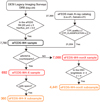 |
Fig. 1 Flowchart of the sample-selection process. |
2 Data and Analysis
2.1 Sample Selection
Figure 1 shows a flowchart of our sample-selection process. Our sample is drawn from the DESI Legacy Imaging Surveys Data Release (DR) 82 (LS8: Dey et al. 2019). LS8 provides optical photometry (g, r, and z) taken from the Dark Energy Camera Legacy Survey (DECaLS) and WISE forced photometry from imaging through NEOWISE-Reactivation (NEOWISE-R; Mainzer et al. 2014) that is measured in the unWISE maps (Lang 2014; Lang et al. 2016) at the locations of the optical sources. WISE provides four-band MIR photometry at 3.4 μm (W1), 4.6 μm (W2), 12 μm (W3), and 22 μm (W4). In addition, LS8 provides photometry, parallaxes, and proper motions from Gaia DR2 (Gaia Collaboration 2018).
We first prepared a WISE 22 μm (W4)-detected sample with a signal-to-noise ratio (SN) of f22 > 5 from LS8. We then excluded the objects for which f22 was severely affected by contributions from their neighborhoods by adopting fracflux_w43 <0.5, which yielded 7780 objects (hereafter referred to as the eFEDS-W4 sample) in the eFEDS foot-print4. Next, we connected the eFEDS-W4 sample and the eFEDS main X-ray catalog with optical-to-MIR counterparts (Salvato et al. 2022) through a unique ID for objects in LS8. The counterparts were assigned after comparing the results of associations obtained using two independent methods: a Bayesian-statistics-based algorithm (NWAY5; Salvato et al. 2018) and a maximum-likelihood method (Sutherland & Saunders 1992) (astromatch6; Ruiz et al. 2018). Both of the methods used LS8; in particular, they were trained on the LS8 properties of a sample of more than 23 000 X-ray sources with secure counterparts (see Salvato et al. 2022, for more details). Based on the comparison of the two methods, each object was set to a counterpart reliability flag (CTP_quality). Salvato et al. (2022) also provided a classification of counterparts (i.e., galactic or extragalactic source) based on optical spectra (if available), Gaia parallaxes, and multicolor information, which can be referred to as a classification flag (CTP_CLASSIFICATION). Before connecting the catalog, we reduced the eFEDS main X-ray sample to 21 934 extragalactic sources that had reliable optical counterparts by adopting CTP_quality ≥2 and CTP_CLASSIFICATION ≥ 2 (see Liu et al. 2022; Salvato et al. 2022, for more details).
As a result of the cross-matching, 692 objects with eROSITA counterparts (hereafter referred to as the eFEDS–W4-X sample) were left; the corresponding sky distribution is presented in Fig. 2. For the 7088 objects that were not detected by eROSITA (hereafter referred to as the eFEDS–W4-nonX sample), we performed the stacking analysis described in Sect. 2.7. We then compiled redshifts and multiwavelength photometric data7 for the eFEDS-W4 sample.
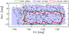 |
Fig. 2 Sky distribution of the 692 eFEDS–W4-X sample (black points) in the eFEDS catalog. The blue-shaded region represents the survey footprint of the HSC-SSP S19A, while the green and red outlines represent those of KiDS DR4 and H-ATLAS DR1, respectively. |
2.2 Spectroscopic Redshifts
Spectroscopic redshifts (zspec8) were compiled from the Two-Micron All-Sky Survey (2MASS; Skrutskie et al. 2006) Redshift Survey (2MRS; Huchra et al. 2012), LAMOST DR4 (Cui et al. 2012), Sloan Digital Sky Survey (SDSS; York et al. 2000) DR16 (Ahumada et al. 2020), the 2dF-SDSS LRG and QSO Survey (2SLAQ; Croom et al. 2009), Galaxy and Mass Assembly (GAMA; Driver et al. 2011) DR3 (Baldry et al. 2018), 6dF Galaxy Survey (6dFGS; Jones et al. 2004) DR3 (Jones et al. 2009), and WiggleZ Dark Energy Survey project DR1 (Drinkwater et al. 2010).
In this work, we focused on objects whose redshifts were spectroscopically confirmed to derive reliable physical quantities and draw an accurate conclusion. Therefore, we only considered 360 objects with zspec (hereafter referred to the eFEDS–W4-X subsample) in Sects. 3 and 4. The redshift distribution of the eFEDS–W4-X subsample is presented in Fig. 3. The eFEDS–W4-X sources distribute the redshifts up to zspec ~ 3.4 with a mean redshift value of 0.63.
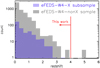 |
Fig. 3 Redshift distribution of the eFEDS–W4-X subsample (blue) and the eFEDS-W4-non X sample (gray). Objects at z < 4 are used for the multiwavelength analysis. |
2.3 Multiwavelength Dataset
2.3.1 UV Data
Far-UV (FUV) and near-UV (NUV) data were taken from the Galaxy Evolution Explorer (GALEX; Martin et al. 2005). We used the revised catalog9 from the GALEX All-Sky Survey (AIS) (GUVcat_AIS; Bianchi et al. 2017), which contains 82992086 sources with 5σ limiting magnitudes of 19.9 in the FUV and 20.8 in the NUV. Before cross-matching, we extracted 80 315723 sources with (i) GRANK ≤ 1 and (ii) fuv_artifact =0 and fuv_flags =0 or nuv_artifact = 0 and nuv_flags = 0, where GRANK, f/nuv_artifact, and f/nuv_flags are the primary-source, artifact, and extraction flags, respectively. This eliminated spurious and duplicate sources (see Sect. 6.2 and Appendix A in Bianchi et al. 2017, for more detail).
2.3.2 u-Band Data
The u-band data were taken from the SDSS and the Kilo-Degree Survey (KiDS; de Jong et al. 2013). We used the SDSS PhotoPrimary table in DR16 (Ahumada et al. 2020) and KiDS DR410 (Kuijken et al. 2019), which contain 469 053 874 and 100 350 871 sources, respectively. The 5σ limiting u-band magnitudes of the SDSS and KiDS DR4 are approximately 22.0 and 24.2, respectively. Because KiDS DR4 does not cover the entire region of the eFEDS (see Fig. 2), we used the SDSS u-band data for objects outside the KiDS footprint. Before cross-matching, we extracted sources with FLAG_GAAP_u = 0 to ensure reliable u-band fluxes for the KiDS sources (see Kuijken et al. 2019) (see also Sect. 2.3.4).
2.3.3 Optical Data
In addition to DECaLS-LS8 (g, r, and z), we used KiDS DR4 (g, r, i, z, and y), where objects with FLAG_GAAP_g/r/i/z/y = 0 were extracted in each band for cross-matching. Additionally, we utilized deep optical data obtained from the Hyper Suprime-Cam (HSC; Miyazaki et al. 2018) Subaru Strategic Program survey (HSC-SSP; Aihara et al. 2018a) (see also Furusawa et al. 2018; Kawanomoto et al. 2018; Komiyama et al. 2018). The HSC-SSP is an ongoing optical imaging survey with five broadband filters (g-, r-, i-, z-, and y-band) and four narrowband filters (see Aihara et al. 2018a; Bosch et al. 2018; Coupon et al. 2018; Huang et al. 2018). In this work, we used S19A wide-layer data obtained from March 2014 to April 2019, for which the survey footprint mostly overlaps with eFEDS (see Fig. 2). The HSC catalog provides forced photometry for the g-, r-, i-, z-, and y-bands with 5σ limiting magnitudes of 26.8, 26.4, 26.4, 25.5, and 24.7, respectively (Aihara et al. 2018b, 2019). These are approximately 15 times deeper than those from LS8. The typical seeing is approximately 0″.6 in the i-band, and the astrometric uncertainty is approximately 40 mas in rms.
We first narrowed down the sample to unique HSC objects with isprimary = True. We then adopted five flags for each band: (i) sdsscentroid_flag =False (i.e., an object has a clean measurement of the centroid position), (ii) pixelflags_edge = False (i.e., an object is not at the edge of a CCD or a co-added patch), (iii) pixelflags_saturatedcenter = False (i.e., the central 3 × 3 pixels of an object are not saturated, (iv) pixelflags_crcenter = False (i.e., the central 3 × 3 pixels of an object are not affected by cosmic rays, and (v) pixelflags_bad=False (i.e., none of the pixels in the footprint of an object is labeled as bad). This left 422 260 020 HSC sources for cross-matching. We employed clean optical data as much as possible for the SED fitting regardless of overlap of the survey footprints for LS8, KiDS, and HSC (see Sect. 2.5).
2.3.4 Near-IR Data
We compiled near-IR (NIR) data from the VISTA Kilo-degree Infrared Galaxy Survey (VIKING; Arnaboldi et al. 2007; Edge et al. 2013). The VIKING data were incorporated into KiDS DR4, for which aperture-matched optical-NIR forced photometry was available. We used J-, H-, and KS -band data with 5σ limiting magnitudes of approximately 23 in J and 22 in KS (Kuijken et al. 2019). Before cross-matching, we extracted sources with FLAG_GAAP_J =0, FLAG_GAAP_H = 0, or FLAG_GAAP_Ks = 0 to ensure reliable photometry (see Kuijken et al. 2019).
Because the KiDS-VIKING catalog (KiDS DR4) partially covers the eFEDS footprint (see Fig. 2), we also used the UKIRT Infrared Deep Sky Survey (UKIDSS; Lawrence et al. 2007) data. We utilized the UKIDSS Large Area Survey DR11plus, which we obtained through the WSA–WFCAM Science Archive11, which contains 88 298 646 sources. The limiting magnitudes of UKIDSS are 20.2, 19.6, 18.8, and 18.2 Vega mag in the Y-, J-, H-, and K-bands, respectively. The UKIDSS catalog contains the Vega magnitudes for each source, and we converted them into
AB magnitudes using offset values Δm (mAB = mVega + Δm) for the Y-, J-, H-, and K-bands of 0.634, 0.938, 1.379, and 1.900, respectively, according to Hewett et al. (2006). Before cross-matching, we extracted 77 276542 objects with (priOrSec ≤ 0 or = frameSetID) and (jpperrbits < 256 or hpperrbits < 256 or kpperrbits < 256) to ensure clean photometry for uniquely detected objects in the same manner as in Toba et al. (2015, 2019b). If an object lay outside the KiDS–VIKING footprint, its NIR flux densities were taken from UKIDSS; otherwise, we always referred to the KiDS–VIKING NIR data.
2.3.5 Far-IR Data
We obtained the FIR data from a project of the Herschel Space Observatory (Pilbratt et al. 2010) Astrophysical Terahertz Large Area Survey (H-ATLAS; Eales et al. 2010; Bourne et al. 2016). This survey provides flux densities at 100 and 160 μm – obtained using a photoconductor array camera and spectrometer (PACS; Poglitsch et al. 2010) – and at 250, 350, and 500 μm – obtained using the Spectral and Photometric Imaging Receiver (SPIRE; Griffin et al. 2010). We used H-ATLAS DR1 (Valiante et al. 2016), which contains 120230 sources in the GAMA fields. The 1σ noise levels for source detection (which include both confusion and instrumental noise) are 44, 49, 7.4, 9.4, and 10.2 mJy at 100, 160, 250, 350, and 500 μm respectively (Valiante et al. 2016).
Because H-ATLAS partially overlaps the eFEDS region (see Fig. 2), we also utilized all-sky data from the AKARI FIR Surveyor (FIS; Kawada et al. 2007) Bright Source Catalog version 2.0 (Yamamura et al. 2018), which includes 918 054 FIR sources. This catalog provides the positions and flux densities in four FIR wavelengths centered at 65, 90, 140, and 160 μm with 5σ sensitivities in each band of approximately 2.4, 0.55, 1.4, and 6.3 Jy, respectively; these are the deepest FIR all-sky data. Following Toba et al. (2017b), we selected 501 444 sources with high detection reliability (GRADE = 3) for cross-matching, that is, sources that were detected in at least two wavelength bands or in four or more scans in one wavelength band.
2.3.6 Cross Identification of Multi-band Catalogs
We cross-identified the GALEX, KiDS-VIKING, SDSS, HSC, UKIDSS, AKARI, and H-ATLAS catalogs with the eFEDS–W4-X sample, always using the LS8 coordinates of the eFEDS–W4-X sample, which we refer to as RA and Dec. Using a search radius of 1″ for KiDS–VIKING, SDSS, and HSC, 3″ for GALEX, 10″ for H-ATLAS, and 20″ for AKARI in the same manner as in Toba et al. (2017b, 2019a,b), we cross-identified 382 (55.2%), 321 (46.4%), 635 (91.8%), 655 (94.7%), 681 (98.4%), 22 (3.2%), and 119 (17.2%) objects with those from GALEX, KiDS–VIKING, SDSS, HSC, UKIDSS, AKARI, and H-ATLAS, respectively. We note that 3/382 (0.8%), 33/635 (5.2%), and 6/681 (0.9%) objects had two candidates within the search radius as counterparts for the GALEX, HSC, and UKIDSS sources, respectively. For cross-matching with other catalogs (SDSS, KiDS-VIKING, AKARI, and H-ATLAS), we obtained one-to-one identification. We found that the multiple fractions of HSC sources were relatively large, possibly due to the high number density of HSC sources. Therefore, we estimated the chance coincidence of cross-matching with the HSC catalog by generating a mock catalog with random positions in the same manner as in Toba et al. (2019b), where the source position in the HSC catalog was shifted from the original position to ± 1° or ±2° along the right assignation direction. Consequently, the chance coincidence was estimated to be <0.2%. We chose the nearest object as the counterpart for this case.
2.4 X-ray Spectral Analysis
Liu et al. (2022) analyzed the X-ray spectra of all eFEDS X-ray sources (see also Nandra et al., in prep.), including those of our eFEDS–W4-X sample. The methodology is summarized below. We extracted the X-ray spectra using srctool v1.63 of the eROSITA Science Analysis Software System (eSASS; Brunner et al. 2022). We used multiple models to fit the spectra of the AGN, and the baseline model was an absorbed power-law. To model bright sources with a soft excess, we added an additional power-law component to the baseline model, creating a “double-power-law” model. To model faint sources for which we could not constrain the spectral shape parameters of the “single-power-law” model, we fixed the power-law slope Γ, the absorbing column density NH, or both at typical values for the sample (Γ = 2.0 and Nh = 0).
We employed the Bayesian method BXA (Buchner et al. 2014; Buchner 2019) to derive constraints on the spectral parameters. For each parameter, we measured the median and 1σ confidence intervals from the posterior distribution. In the spectral analysis, we always modeled the galactic absorption using NH, as measured by the HI4PI (HI4PI Collaboration 2016), and adopted the photoionization cross-sections provided in Verner et al. (1996) and the abundances provided in Wilms et al. (2000).
Based on a detailed analysis of the parameter posterior distributions, Liu et al. (2022) provided an NH measurement flag for each source, dividing the sources into four classes: (1) uninformative, (2) unobscured, (3) mildly-measured, and (4) well-measured. Following Liu et al. (2022), we considered unobscured sources with a median log NH < 21.5 cm−2 as X-ray unobscured (or type 1) AGN and mildly-measured or well-measured sources with a median log NH ≥ 21.5 cm−2 as X-ray obscured (or type 2) AGN. For each source, based on the parameter constraints of the data, we chose the most suitable model to estimate the X-ray luminosities. Generally, we adopted the flexible double-power-law model for high-quality data and the single-power-law model with one or more parameters fixed for low-quality data. However, in the case of X-ray type 2 AGN, we adopted the single-power-law model instead of the flexible double-power-law model to avoid strong degeneracy between the soft excess and the absorption. A full description of the X-ray data reduction and analysis is provided in Liu et al. (2022).
2.5 SED Fitting with X-CIGALE
To derive the physical properties of our sample, we performed SED fitting in which we employed a new version of the Code for Investigating GALaxy Emission (CIGALE; Burgarella et al. 2005; Noll et al. 2009; Boquien et al. 2019), known as X-CIGALE12 (Yang et al. 2020). X-CIGALE implements an X-ray module that enables fitting from X-ray to FIR wavelengths in a self-consistent framework by considering the energy balance between the UV–optical and IR wavelengths. This code can handle many parameters, such as the star formation history (SFH), single stellar population (SSP), attenuation law, AGN emission, dust emission, and radio synchrotron emission (see e.g., Boquien et al. 2014, 2016; Buat et al. 2015; Lo Faro et al. 2017; Toba et al. 2019b, 2020c). The parameter ranges used in the SED fitting are listed in Table 1.
We assumed a SFH comprising two exponentially decreasing SFRs with different e-folding times (e.g., Ciesla et al. 2015, 2016). We chose the SSP model of Bruzual & Charlot (2003), assumed the IMF of Chabrier (2003), and used the standard nebular emission model included in X-CIGALE (see Inoue 2011).
For attenuation by the dust associated with the host galaxy, we utilized a starburst attenuation curve (Calzetti et al. 2000; Leitherer et al. 2002) in which we parameterized the color excess of the nebular emission lines [E(B − V)lines], extended with the Leitherer et al. (2002) curve. The color excess of stars, E(B − V)*, can be converted from E(B − V)lines by assuming a simple reduction factor  (Calzetti 1997).
We modeled the IR emission from dust (reprocessed from the absorbed UV–optical stellar emission) using the dust templates provided by Dale et al. (2014). This model is formulated as dMd (U) ∝ U−αdU, where Md is the dust mass, U is the intensity of the radiation field, and α is a dimensionless parameter.
We modeled the AGN emission using SKIRTOR (Baes et al. 2011; Camps & Baes 2015; Stalevski et al. 2012, 2016), a two-phase medium torus model with high-density clumps embedded in a low-density component, with seven parameterized quantities (see Stalevski et al. 2016; Yang et al. 2020, for details). As parameters, we used the torus optical depth at 9.7 μm (τ9.7), the torus density radial parameter (p), the torus density angular parameter (q), the angle between the equatorial plane and the edge of the torus (Δ), the ratio of the maximum to minimum radii of the torus (Rmax/Rmin), the viewing angle (θ), and the AGN fraction of the total IR luminosity (fAGN), all of which are listed in Table 1.
We modeled the X-ray emission using a combination of (i) an AGN with a power-law photon index (Γ) defined as fv ∝ ν1−Γ, (ii) low-mass X-ray binaries (LMXBs), (iii) high-mass X-ray binaries (HMXBs), and (iv) hot gas. The X-ray emissions from the LMXBs and HMXBs were connected to the assumed SFH and SSP, and the hot-gas emission was modeled using free-free and free-bound emission from optically-thin plasma with Γ = 1. To connect the continuum emission from X-rays with other wavelengths, X-CIGALE employs an empirical relation between αOX and L2500Å (Just et al. 2007), where L2500Å is the intrinsic (dereddened) AGN luminosity density at 2500 Å, and αOX is the SED slope between 2500 Å and 2 keV. The derived value of αOX is allowed to deviate from that expected from the αOX−L2500Å relation (Just et al. 2007) by up to ~2σ (i.e., |Δ αOX|max = |αOX − αOX (L2500Å)|max = 0.2), following Yang et al. (2020).
Using the parameter settings listed in Table 1, we fitted the stellar, nebular, AGN, SF, and X-ray components to at most 25 photometric points from X-ray to FIR wavelengths of the eFEDS-W4-X subsample. Below, we explain the photometry used for each dataset employed for the SED fitting. For the X-ray data, we used FluxCorr_S and FluxCorr_H, which are the absorption-corrected fluxes in the 0.5–2 and 2–10 keV bands, respectively (see Liu et al. 2022). For the UV data, we used FUV_mag and NUV_mag, which are the GALEX calibrated magnitudes in the FUV and NUV wavelengths (see Bianchi et al. 2017). For the optical (DECaLS) and MIR (unWISE) data in LS8, we used forced photometry at the positions of the optical counterparts (see Dey et al. 2019). For the SDSS and HSC optical data, we used the cModel magnitude, whose HSC five-band photometry was forced photometry (see e.g., Bosch et al. 2018). For the optical–NIR data taken from KiDS, we used aperture-matched forced photometry at the positions of the optical counterparts (MAG_GAAP_u/g/r/i/z/y/j/h/ks) (see Kuijken et al. 2019). For the NIR data taken from UKIDSS, we utilized the Petrosian (1976) magnitudes (j/h/kPetroMag) (see also Lawrence et al. 2007). For the FIR data, we used the default fluxes (i.e., FLUX_65/90/140/160 for AKARI and F1SS/16S/25S/35S/5SSB for Herschel) (see Valiante et al. 2016; Yamamura et al. 2018). The flux densities at 250, 350, and 500 μm can be boosted, especially for faint sources (known as flux boosting or flux bias), which are caused by confusion noise and instrument noise. Hence, we corrected this effect using the correction term provided in Table 6 of Valiante et al. (2016). We corrected all the flux densities from X-ray to MIR wavelengths for galactic extinction.
Further, we examined the consistency of optical and NIR photometry for objects detected using the same band taken from different surveys (e.g., KiDS–VIKING u-band and SDSS u-band). For the u-band magnitude, the median value of the difference between KiDS-VIKING and SDSS was 0.08 mag. For the optical data, the median values of the differences between (i) KiDS–VIKING and LS8 (g, r, and z), (ii) HSC and LS8 (g, r, and z), and (iii) KiDS–VIKING and HSC (g, r, i, z, and y) were typically 0.09, 0.05, and 0.03 mag, respectively, which is acceptable in this work. However, the median values of the differences between KiDS-VIKING and UKIDSS for the J, H, and K-bands were 0.12, 0.15, and 0.11 mag, respectively, which is a relatively large discrepancy. Although the differences in optical and NIR photometry did not significantly affect the resulting physical values, as discussed in Sect. 3.2, we should consider the possible systematic differences in NIR photometry in this work.
Following Toba et al. (2019b), we used the flux density at a given wavelength when SN was greater than 3 at that wavelength. If an object was undetected, we placed 3σ upper limits at those wavelengths13. Although the photometry employed in each catalog is different, they may trace the total flux densities. Therefore, the influence of differences in the photometry is expected to be small. Nevertheless, it is worth addressing whether physical properties are actually estimated in a reliable way given the uncertainties in each source of photometry, which we discuss in Sect. 3.2.
Parameter ranges used in the SED fitting with X-CIGALE.
2.6 2D Image Decomposition
We performed 2D image analysis in the same manner as in Li et al. (2021), which involved an automated fitting routine based on the image modeling tool Lenstronomy (Birrer et al. 2015; Birrer & Amara 2018) to decompose the image into a point source and a host-galaxy component. A full description is provided in Ding et al. (2020) and Li et al. (2021). We briefly summarize the analysis here. For image decomposition, we used a cut-out image obtained from the HSC i-band14, for which the image size was automatically optimized in the procedure.
We performed 2D brightness profile fitting for the background-subtracted cut-out images using a point spread function (PSF) (for the point source) and a single elliptical Sérsic model (for the host galaxy) to determine galactic structural properties, such as the Sérsic index (n) and half-light radius (Re) as well as the flux densities of the central point source and the host galaxy (see Eq. (1) in Li et al. 2021). The best-fit model image was obtained using χ2 minimization based on the particle swarm optimization algorithm (Kennedy & Eberhar 1995). The 1σ error of the best-fit structural parameters and the flux density of each component could be inferred through the Markov-chain Monte Carlo (MCMC) sampling procedure in Lenstronomy (Foreman-Mackey et al. 2013). However, we eventually employed a 10% error for each quantity because the derived errors based on the MCMC procedure were found to be unrealistically small, possibly due to adopting a fixed PSF in our 2D profile fitting (see Sect. 3.1 in Li et al. 2021).
Figure 4 presents examples of quasar-host decomposition based on the HSC i-band image. We found that the reduced χ2  of the profile fitting worsened for objects at z < 0.1, probably because the radial profile of a low-z object is often difficult to explain with a single Sérsic model (Li et al. 2021). Moreover, it was difficult, even when using the HSC data, to decompose the host emission for objects at z > 1 given the angular resolution of the HSC. Following Li et al. (2021), we used products (e.g., host flux densities) for objects at 0.2 < z < 0.8 with reduced
  to ensure reliable host properties (see Sect. 4.2).
2.7 X-ray Stacking Analysis
Among the 7088 objects in the eFEDS–W4-nonX sample, 5822 objects were in the survey footprint of the HSC-SSP. Because 4288/5822 (~74%) sources did not have zspec, we computed photometric redshifts (zphoto) for them. We utilized zphoto calculated using the machine learning code Deep Neural Network Photo-z (DNNz; Nishizawa et al., in prep.). The DNNz comprises multilayered perceptrons with four fully connected hidden layers, with each layer having 100 nodes. For the inputs, we have used the cmodel fluxes and PSF-convolved aperture fluxes for five HSC broadband filters, translated into asinh magnitudes (Lupton et al. 1999), as well as the sizes derived from second-order moments for each filter. The output is the probability of an individual galaxy being in a certain redshift bin, with redshifts divided linearly from z = 0–7. With the spectroscopic-redshift sample and the high-quality photometric-redshift sample in COSMOS, which are summarized in Nishizawa et al. (2020), the code is trained so that the output probability approaches a Dirac delta function at the true redshift.
Figure 5 shows a comparison between zspec and zphoto for the eFEDS-W4-nonX sample, in which we compiled zspec from the SDSS DR15, GAMA DR3, and WiggleZ DR1. The resulting accuracy of zphoto, the normalized median absolute deviation defined as σΔz/(1+zspec) = 1.48 × median(|Δz|/(1+zspec)) (e.g., Ilbert et al. 2006), is 0.03. The outlier fraction (i.e., the fraction of sources with |Δz|/(1+zspec) > 0.15) is 3.98%, which is acceptable in this work (see also Sect. 2.4). However, we have verified the performance of zphoto only for the objects at z < 4. Therefore, we only considered the objects at z < 4 to ensure the reliability of zphoto for these high-z sources (see Fig. 3). Moreover, we adopted brightblob15 ≠ 3 to extract extragalactic objects with reliable redshifts (see also Sect. 2.2). Accordingly, 4441 objects (hereafter referred to as the eFEDS–W4-nonX subsample) remained for the stacking analysis. The sample was separated into five subsamples using the following redshift bins: (i) z < 0.1, (ii) 0.1 < z < 0.25, (iii) 0.25 < z < 0.5, (iv) 0.5 < z < 1.0, and (v) z > 1.0, and we then stacked each subsample as follows.
We first masked the previously detected sources using the position from the catalog (Salvato et al. 2022) in the X-ray images (30″ radius for point source and a spatial extent for extended sources). This ensured that we could properly characterize the background. We performed masking on four bands, that is, full (0.2–10 keV), soft (0.2–0.6 keV), mid (0.6–2.3 keV), and hard (2.3–5.0 keV) (see Brunner et al. 2022). We then stacked images in all four bands by taking the mean of the inverse exposure weighted 2′ × 2′ cutouts centered on each LS8 position, essentially creating count-rate stacked images. To not overly weigh sources at the edges of the field, we required a minimum exposure time of 180 s, which reduced the number of stacked sources by 3–5%, with the larger percentage in the hard band, which experienced a lot of vignetting (see Sect. 3.3).
Thereafter, we attempted to detect the source in the stacked image by PSF-matching the center to the background. We selected a boundary SN of 1.8 as our boundary, which corresponded to a matched detection significance of 5.0. Lastly, we determined the (limiting) fluxes above the background using the following energy conversion factors: full, 5.03 × 10¹¹; soft, 9.61 × 10¹¹; mid, 1.06 × 10¹²; and hard, 1.13 × 10¹³. They were calculated using an absorbed power-law model with log Nh = 20 cm−2 and Γ of 1.7.
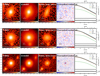 |
Fig. 4 Examples of quasar-host decomposition based on the HSC i-band image. From left to right: (i) the observed HSC i-band image, (ii) the best-fit point source + host galaxy model, (iii) the data minus the point source model (the pure-galaxy image), (iv) fitting residuals divided by the variance map, and (v) one-dimensional surface brightness profiles (top) and the corresponding residuals (bottom). |
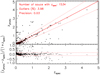 |
Fig. 5 Comparison between zspec and zphoto for the eFEDS-W4-nonX sample. The red solid line represents zspec = zphoto. The red dotted lines denote Δz/(1+zspec) = ±0.15. The bottom panel shows Δz/(1+zspec) as a function of zspec. |
3 Results
As described in Sects. 2.2 and 2.7, we conservatively narrowed down the eFEDS–W4 sample to 360 objects in the eFEDS–W4-X subsample and to 4441 objects in the eFEDS–W4-nonX subsample with z < 4 to ensure the reliability of the determined physical quantities (see also Fig. 1). We present the results of X-ray spectral analysis, SED fitting, and X-ray stacking analysis, which characterize eROSITA-detected and -undetected WISE galaxies and AGN.
3.1 Results of X-ray Spectral Analysis
Figure 6 presents examples of the X-ray spectra. We estimated the absorption-corrected X-ray luminosities in the rest-frame soft (0.5–2 keV) band (LX (0.5–2 keV)) and hard (2–10 keV) band (LX (2–10 keV)) for all the 360 objects. However, for 21 objects (with a class of uninformative), LX has large uncertainties because the shapes of the X-ray spectra have been fixed (see Liu et al. 2022). We therefore exclude them from the following analysis. The luminosities of these 360–21 = 339 objects are presented as a function of redshift in Figs. 7 and 8. The mean values and standard deviations of these luminosities are log LX (0.5–2 keV) = 43.4 ± 1.41 erg s−1 and log LX (2–10 keV) = 43.4 ± 1.37 erg s−1. If we consider objects with log LX (2–10 keV) > 42 erg s−1 as AGN (e.g., Barger et al. 2005), 278/339 (~82%) objects satisfy the criterion. We find that approximately 86 and 14% of X-ray AGN are classified as X-ray type 1 and type 2 AGN according to the best-fit model (see Sect. 2.4).
We present NH for 339 objects in the eFEDS–W4-X subsample in Fig. 9. The mean value and standard deviation of log NH for our AGN sample is log NH = 20.6 ± 0.69 cm−2, and the mean value and standard deviation of the photon index is Γ = 2.0 ± 0.3; both are in good agreement with a previous work on X-ray AGN (Trump et al. 2011).
3.2 Results of SED Fitting
Figure 10 shows examples of the SED fits obtained with X-CIGALE. We confirmed that 197/360 (~55%) objects reduced χ2 ≤ 3, while 263/360 (~73%) objects have reduced χ2 ≤ 5. This suggests that the data are moderately well fitted by X-CIGALE with a combination of stellar, nebular, AGN, SF, and X-ray components. Hereafter, we focus on the subsample of 263 eFEDS–W4-X sources with reduced χ2 smaller than 5 for the SED fitting, in the same manner as in Toba et al. (2019b, Toba et al. 2020c).
Figure 11 shows the IR luminosity (LIR). LIR is traditionally defined as the luminosity integrated over the wavelength range 8–1000 μm (e.g., Sanders & Mirabel 1996; Chary et al. 2004). However, because this definition includes contributions from stellar emissions, we did not adopt any wavelength boundary for the integration range. Instead, we employed a physically oriented approach to estimate LIR as a function of redshift based on X-CIGALE by considering the energy re-emitted by dust that has absorbed UV–optical emission from SF–AGN (see e.g., Toba et al. 2020b, Toba et al. 2021b). We found that approximately 67% of our samples are ultraluminous IR galaxies (ULIRGs: Sanders & Mirabel 1996) and 24% are hyperluminous IR galaxies (HyLIRGs: Rowan-Robinson 2000), with LIR > 1012 and >1013 L⊙, respectively. This suggests that a large fraction of X-ray-detected WISE 22 μm sources are ULIRGs and may even be HyLIRGs. Furthermore, we discovered two candidates (0.8% of our sample) that are extremely luminous IR galaxies (ELIRGs: Tsai et al. 2015), with LIR greater than 1014 L⊙; indeed, Toba et al. (2021b) confirm that the object named WISEJ0909+0002 at zspec = 1.871 is an ELIRG. However, we note that CIGALE would overestimate FIR emission from SF for objects that do not have FIR photometry (e.g., Masoura et al. 2018). Only 26/263 objects in the eFEDS–W4–X subsample were detected by Herschel or AKARI (see objects with red circles in Fig. 11). The remaining 237 sources had upper limits given by Herschel and AKARI, which would be insufficient to constrain the FIR SEDs. We confirmed that the mean value of LIR for these objects without FIR detections is log (LIR/L⊙) = 12.4, which is approximately 0.4 dex larger than that of the objects with FIR detections, which should be kept in mind as the potential systematic uncertainty of LIR (and SFR) in this work.
We performed a mock analysis to check whether the physical properties can be reliably estimated in the same manner as in Toba et al. (2019b, 2020c). To create the mock catalog, X-CIGALE first uses the photometric data for each object based on the best-fit SED and then modifies the photometry for each one by adding a value taken from a Gaussian distribution with the same standard deviation as the observation. This mock catalog is then analyzed in exactly the same way as for the original observations (i.e., the mock analysis uses the same simulation model as the fitting model) (see Boquien et al. 2019, for more details). This analysis also enables us to examine the influence of photometric uncertainties on the derived physical quantities (see Sect. 2.5).
Figure 12 presents the differences in E(B − V)*, the stellar mass, the SFR, and LIR derived from X-CIGALE in this work and those derived from the mock catalog as a function of redshift. The mean values are ΔE(B − V)* = 0.05, ∆ log M* = 0.004, ∆ log SFR = 0.16, and ∆ log LIR = 0.11. Although there is no significant dependence on redshift, the relatively large offsets for SFR and LIR suggest that these quantities may be sensitive to photometric uncertainties. This may be a limitation of our SED fitting method given the limited number of data points. This possible uncertainty should be kept in mind in the following discussion.
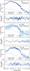 |
Fig. 6 Examples of the X-ray spectra from eROSITA. The best-fit model and its 99% confidence interval are displayed as blue-shaded regions. For each source, the lower panel shows comparison of the data with the best-fit model in terms of (data–model)/error, where error is calculated as the square root of the model predicted number of counts. |
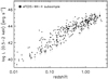 |
Fig. 7 Absorption-corrected X-ray luminosity in the 0.5–2 keV band for the 339 objects in the eFEDS–W4-X subsample as a function of redshift. |
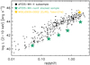 |
Fig. 8 Absorption-corrected X-ray luminosity in the 2–10 keV band for the 339 objects in the eFEDS–W4-X subsample as a function of redshift. The green stars represent the eFEDS–W4-nonX subsample used in the X-ray stacking analysis, for which we calculated LX by assuming NH = 0 cm−2 and Γ = 2.0. The yellow star denotes the ELIRG (WISEJ0909+0002) reported in Toba et al. (2021b). |
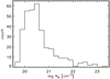 |
Fig. 9 Histogram of hydrogen column density (NH) measured from the eROSITA X-ray spectra for 339 objects. |
3.3 Results of X-ray Stacking Analysis
Figure 13 shows the stacked images in the observed frame of all the eFEDS–W4-nonX samples as functions of redshift. The resulting X-ray flux in each band is tabulated in Table 2. X-ray photons are detected in the 0.2–0.5-, 0.6–2.3-, and 0.2–10-keV bands for objects at z < 1, while 3σ upper limits are obtained for the 2.3–5.0-keV band regardless of redshift. Using the stacked spectra at these five redshift bins, we estimated the mean intrinsic (absorption-corrected) 2–10 keV luminosities of the eFEDS–W4-nonX subsamples. To convert the observed count rates into luminosities, we consider an absorbed power-law model with a 1% unabsorbed scattered component, assuming Γ = 2.0 and four different values of absorption at the source redshift, Nh = 0, 1022, 1023, and 1024 cm−2, in addition to the Galactic absorption of Nh = 2.58 × 1020 cm−2 (Liu et al. 2022). For simplicity, we ignore other components such as opticallythin thermal emission and emissions from X-ray binaries in the host galaxies. Thus, our estimates of the AGN luminosities must be taken to be upper limits. We basically refer to the count rates in the 0.6–2.3 keV band, where eROSITA is the most sensitive and all the stacked spectra are significantly detected. If the 3σ upper limit of the 2.3–5.0 keV count rate gives a smaller luminosity than the estimate from the 0.6–2.3 keV count rate, then we adopt the former value as an upper limit (which is the case only for z < 0.1 and NH = 1023 cm−2). The results are summarized in Table 3. It is noteworthy that the presence of obscured AGN with L2–10 > 1042 erg s−1 in these X-ray-undetected sources is possible, although the inferred mean AGN luminosity is highly dependent on the assumed absorption column density.
We present the resulting values of LX for the eFEDS–W4-nonX stacked sample as a function of redshift in Fig. 8, where LX is plotted assuming NH =0 cm−2. We observe that the values of LX for this stacked sample are smaller than those for the eFEDS–W4-X sample. Given the fact that the majority of the eFEDS–W4-X sample is expected to be unobscured AGN (see Sect. 3.1 and Fig. 9), this result indicates that the estimates of LX for the eFEDS–W4-nonX stacked sample are reasonable. Figure 11 presents the resulting values of LIR for the eFEDS–W4-nonX subsample as a function of redshift. Because LIR can be estimated for individual sources in the sample (see below), we plotted the mean values and standard deviations of log LIR for each redshift bin in addition to plotting individual sources. We can see that the values of LIR for the eFEDS–W4-nonX sub-sample are smaller than those for the eFEDS–W4-X subsample, although there is large dispersion. This is possibly because our eFEDS–W4-X subsample was limited to objects with zspec; thus, their LIR would be biased toward higher luminosity, which is confirmed via the stacked SED described below.
To compare the shapes of the SEDs between the eFEDS–W4 samples with and without eROSITA detections, we performed SED fitting for the eFEDS–W4-nonX subsample. We compiled the multiwavelength data and performed SED fitting to the UV-FIR data in the same manner as described in Sects. 2.3 and 2.5. We created the composite SED by stacking the best-fit SEDs for all the objects. The composite SEDs of the eFEDS–W4-X and eFEDS–W4-nonX subsamples are displayed in Fig. 14, where we do not use ~0.005–0.1 μm for stacking the SEDs because there are no data points in that wavelength range. No significant differences are observed in the NIR and FIR SEDs among these sources.
In the optical region, however, the eFEDS–W4-X subsample exhibits a power-law SED caused by emission from the AGN accretion disk, while the eFEDS–W4-nonX subsample exhibits Balmer and 4000 Å break features caused by emission from the AGN host. In addition, the strength of the silicate feature at 9.7 μm (i.e., τ9.7) is larger for the eFEDS–W4-nonX subsample than for the eFEDS–W4-X subsample (see the inset of Fig. 14). The power-law feature of the eFEDS–W4-X subsample is consistent with the fact that the majority of the sample comprises X-ray type 1 AGN (see Sect. 3.1). However, some eFEDS-W4-nonX sources may be dust-obscured type 2 AGN, including CT-AGN (see Sect. 4.3). This is supported by the relatively strong 9.7 μm silicate dust absorption seen in their composite SED. Nevertheless, this is inconclusive because NH cannot be constrained for the eFEDS–W4-nonX subsample given the current dataset.
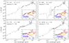 |
Fig. 10 Examples of SED fitting. The black points are photometric data, and the gray solid line represents the resulting best-fit SED. The inset shows the SED at 0.1–500 μm, with the contributions from the stellar, AGN, and SF components to the total SED shown as blue, yellow, and red lines, respectively. |
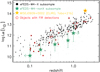 |
Fig. 11 IR luminosity as a function of redshift. The green stars represent the eFEDS–W4-nonX subsample, for which the values of LIR are the mean and standard deviation for sources (indicated by green dots) in each redshift bin, as given in Table 2. The yellow star represent the ELIRG (WISEJ0909+0002) reported in Toba et al. (2021b). Objects with red circles have FIR detections from Herschel or AKARI. |
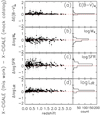 |
Fig. 12 Differences in E(B − V),, the stellar mass (M*), the SFR, and LIR derived from X-CIGALE in this work and those derived from the mock catalog. (a) ΔΕ(Β − V),, (b) M*, (c) SFR, and (d) LIR as functions of redshift. Right-hand panels: histograms of each quantity. The red dotted lines correspond to Δ = 0. |
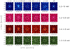 |
Fig. 13 Stacked X-ray images (2′ × 2′) of the eFEDS–W4-nonX samples as a function of redshift bin. From left to right: bins are z < 0.1, 0.1 < z < 0.25, 0.25 < z < 0.5, 0.5 < z < 1.0, z > 1.0, and all the samples. The energy bands (in the observed frame) of the subsample are 0.2–10, 0.2–0.5, 0.6–2.3, and 2.3–5.0 keV from top to bottom. |
X-ray fluxes of the stacked eFEDS–W4-nonX subsample.
4 Discussion
4.1 Relationship Between MIR and X-ray Luminosities
The MIR luminosity (e.g., the 6 μm luminosity L6) and the hard X-ray luminosity [e.g., LX (2–10 keV)] of the AGN are positively correlated over a wide luminosity range, regardless of the AGN type (e.g., Gandhi et al. 2009; Asmus et al. 2015; Mateos et al. 2015; Stern 2015; Chen et al. 2017; Ichikawa et al. 2017; Toba et al. 2019a). Because our AGN sample has a wide range of X-ray and IR luminosities, as shown in Figs. 8 and 11, it is worth investigating whether our eFEDS–W4-X sample also follows this relationship. We show the resulting relationship between the rest-frame 6 μm luminosity and the rest-frame 2–10 keV luminosity in Fig. 15. The plotted points represent X-ray AGN (with log Lx (2–10 keV) > 42 erg s−1) with reliable Lx (i.e., which are classified as unobscured, mildly-measured, or well-measured). The X-ray luminosity is corrected for absorption (see Sect. 2.4), while the 6 μm luminosity is corrected for contamination from the host galaxy in the same manner as in Toba et al. (2019a).
We also plot the best-fit L6−Lx relation for AGN samples taken from the Bright Ultra-hard XMM–Newton Survey (BUXS; Mateos et al. 2015), the SDSS quasars (Stern 2015), and data compiled for some deep fields (Chen et al. 2017). We performed a linear regression in log–log space for the eFEDS–W4-X AGN sample by considering the errors in L6 and Lx obtained from a Bayesian maximum-likelihood method provided by Kelly (2007). The resulting linear relation is as follows:
 (1)
(1)
and the correlation coefficient is r ~ 0.91, which confirms the tight correlation between L6 and LX for our X-ray AGN sample. We note that the slope of this relation (i.e., Lx/L6) is flatter than for the X-ray AGN detected by the ROSAT all-sky survey (RASS) reported in Toba et al. (2019a), while it is steeper than that of the AGN detected by deep X-ray observations such as XMM-COSMOS (Chen et al. 2017). Chen et al. (2017) suggested that X-ray flux limits may affect the slopes, as the ratio Lx/L6 determined using shallower X-ray flux limits tends to be larger. Because the flux limit of eROSITA–eFEDS is more than one order of magnitude deeper than that of RASS, while it is about one order of magnitude shallower than that of XMM–COSMOS (although the survey area of eFEDS is about 65 times larger than XMM–COSMOS), this result may support the explanation suggested by Chen et al. (2017).
We also plot the 6 μm and hard X-ray luminosities of the eFEDS–W4-nonX stacked sample. The mean values of Lx for this stacked sample (with NH = 0–1023 cm−2) in each redshift bin, and their standard deviations, are plotted on the y-axis. The weighted means and standard deviations of the L6 values in each redshift bin are plotted on the x-axis. We find that the best-fit slope of the stacked AGN sample with log Lx > 42 erg s−1 is −0.47, which is consistent with that for the XMM–COSMOS sample, which further supports the explanation suggested by Chen et al. (2017).
Absorption-corrected X-ray luminosities in the 2–10 keV band of the stacked eFEDS–W4-nonX subsample.
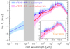 |
Fig. 14 Composite SEDs of the eFEDS-W4-X subsample (blue) and eFEDS-W4-nonX subsample (red). The shaded regions represent the standard deviations of the stacked SED medians. There are no data points in the gray region, and composite SEDs are excluded. The inset displays a magnified view of the rest-frame optical-to-FIR SEDs. |
4.2 Structural Properties of AGN Host Galaxies
In Sect. 2.6, we described the 2D image decomposition of the HSC images used to distinguish emission from a central point source and an extended component. This analysis provides flux-density data for the AGN and its host separately, which enables us to estimate the stellar mass reliably without it being affected by the AGN emission.
4.2.1 Correlation of the AGN Fraction Derived from X-CIGALE and 2D Image Decomposition
Figure 16 shows the relationship between the point-source fraction of the i-band flux density  derived from the image decomposition and the AGN fraction derived from the SED fitting with X-CIGALE. The AGN fraction is defined as Lir(AGN)/Lir. The sources plotted in this figure are limited to those with reduced
  at 0.2 < z < 0.8 (see Sect. 2.6). In particular, it is worth investigating how the AGN fraction froman optical decomposed-image point of view is associated with that from the IR SED-fitting point of view for type 1 AGN. Hence, we focus on X-ray type 1 AGN, as classified in Sect. 3.1. We find these quantities to be weakly correlated, with correlation coefficients r ~ 0.26 where r is derived using the Bayesian method (Kelly 2007) (see Sect. 4.1). This result indicates that the 2D image decomposition and SED fitting with X-CIGALE work consistently to evaluate the contributions of the AGN to the optical and IR bands.
In addition, we find that even for objects with  0.8 the AGN fraction rarely exceeds 0.6, which is consistent with what is reported in previous works (e.g., Lyu et al. 2017; Ichikawa et al. 2019). The SF activity is expected to contribute significantly to the IR fluxes for luminous AGNs, suggesting an AGN–SF connection; that is the co-existence of gas consumption into SF and SMBHs (see e.g., Imanishi et al. 2011; Stemo et al. 2020).
Further, we compare the AGN fraction measured at the restframe i-band from the best-fit SEDs and image decomposition  . We observe a weak correlation with correlation coefficient r ~ 0.2 for X-ray type 1 AGN. By contrast, we observe a moderately strong correlation (r ~ 0.3) for X-ray type 2 AGN, which may indicate that SED decomposition (to distinguish between emissions from the accretion disk and stellar component) in the optical bands has a large uncertainty, particularly for type 1 AGN (see Sect. 4.2.2).
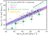 |
Fig. 15 Relationship between the rest-frame 6 μm luminosity contributed by AGN and the absorption-corrected, rest-frame 2–10-keV luminosity for the eFEDS–W4 sample. The best-fit linear function in log–log space and its 1er dispersion are shown as the solid blue line and the shaded blue band, respectively. The cyan line represents the best-fit for an X-ray-selected AGN sample from the BUXS catalog (Mateos et al. 2015). The orange and magenta lines show two-dimensional polynomial and bilinear relations from Stern (2015) and Chen et al. (2017), respectively. The green stars represent the eFEDS–W4-nonX subsample used for the X-ray stacking analysis in which we obtained the weighted mean and standard deviation in each redshift bin by taking into account the uncertainties in NH (NH = 0–1023 cm−2). The black dotted line represents a one-to-one correspondence between the 6 μm and 2–10 keV luminosities. The yellow star denotes the ELIRG (WISEJ0909+0002) reported in Toba et al. (2021b). |
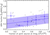 |
Fig. 16 AGN fraction (LIR(AGN)/LIR) of the eFEDS–W4-X sample at 0.2 < z < 0.8 versus the point-source fraction of the i-band flux density |

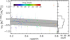 |
Fig. 17 Ratio of the stellar mass derived from SED fitting with all the data |


4.2.2 Consistency of Stellar Mass Based on the Host Flux Densities
Many works have reported that estimates of stellar masses based on SED fitting – particularly for type 1 AGN – may have large uncertainties because it is often difficult to distinguish the accretion disk and the stellar component given a limited number of photometric bands (see e.g., Merloni et al. 2010; Bongiorno et al. 2012; Toba et al. 2018). This motivated an investigation to determine how to estimate securely the stellar mass derived from SED fitting with X-CIGALE. The host flux information provided by the 2D image decomposition enables us to estimate the stellar mass reliably (e.g., Li et al. 2021). Accordingly, we performed SED fitting to the HSC five-band photometry of each AGN host to obtain the stellar mass  without being affected by AGN emission. To obtain a better estimate of the stellar mass, we parameterized the SFH and SSP over narrow intervals.
Figure 17 shows a comparison of the stellar mass derived from the SED fitting with all the data ( see Sect. 2.5) and from the HSC five-band flux density for the AGN host from the eFEDS–W4-X sample at 0.2 < z < 0.8 as a function of red-shift. This comparison shows that the stellar mass derived in this work may be systematically underestimated by ~0.3 dex. The resulting correlation coefficient (r = − 0.20 ± 0.17) indicates that this offset does not considerably depend on redshift, at least up to z = 0.8. Nevertheless, a faint (i-mag > 23) object at z > 0.7 deviates considerably from the typical offset, which should be kept in mind as indicative of the uncertainty in the stellar mass.
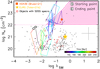 |
Fig. 18 Relation between log NH and λEdd for the eFEDS–W4 sample. The yellow star represents the ELIRG (Toba et al. 2021b), and the orange square shows the location of XID439 (see text). Objects with red circles have optical spectra from SDSS DR16. Typical uncertainties in log NH and λEdd are shown at the bottom right. The dotted line denotes the effective Eddington limit ( |


4.3 Evolutionary Stage of the eROSITA-detected MIR Galaxies
Finally, we discuss the evolutionary phase of the eFEDS–W4 sample using the Eddington ratio (λEdd) and NH. The Eddington ratio is defined as λEdd = Lbol/LEdd, where Lbol is the bolometric luminosity and LEdd is the Eddington luminosity. For 32 quasars that are cataloged in the SDSS DR16 quasar catalog (Lyke et al. 2020), we estimate the single-epoch virial black-hole mass (MBH) based on a few recipes using the continuum luminosities at 1450, 3000, and 5100 Å, as well as the full width at half maximum (FWHM) of the C IV, Mg II, and Hβ lines (Vestergaard & Peterson 2006; Shen et al. 2011) (see also Sect. 5.2 in Rakshit et al. 2020). We employed the quasar spectral-fitting package (QSFit v1.3.0; Calderone et al. 2017) to determine the line widths and continuum luminosities in the same manner as in Toba et al. (2021a). The values of MBH for the remaining sources are obtained from the stellar mass using an empirical relation for AGN up to z ~ 2.5 provided in Suh et al. (2020). We use  as the stellar mass unless
  is available. The uncertainties in the stellar mass and the intrinsic scatter of M*−MBH (~0.5 dex) reported in Suh et al. (2020) are propagated to the uncertainty of the converted MBH. The value of Lbol is estimated by integrating the best-fit SED template for the AGN component output from X-CIGALE (see e.g., Toba et al. 2017c). The uncertainty in Lbol is calculated by error propagation of the uncertainty in the AGN luminosity.
Figure 18 shows the relation between λEdd and NH for the eFEDS–W4-X subsample, which tells us how the obscuration of the AGN is associated with mass accretion onto the SMBH (see e.g., Fabian et al. 2009). Objects in the pink shaded region in Fig. 18 are expected to blow out the surrounding gas and dust by strong radiation pressure (Fabian et al. 2006, 2009; Ishibashi et al. 2018). We estimate the fraction of objects located in this “blow-out region” (fblow–out). Note that obtained values of NH and λEdd have quite large uncertainties (0.5–1 dex). In addition, only 12% of the eFEDS–W4-X subsample plotted in Fig. 18 has a spectroscopically derived λEdd, and λEdd for the majority of the sample is empirically estimated by assuming an M*−MBH relation. Therefore, we take into account the uncertainties in NH and λEdd as well as statistical errors in the fraction through Monte Carlo randomization to estimate fblow–out. We find that fblow–out = 5.0 ± 2.5% (see Fig. 19). We note that this value should be considered a lower limit because we only investigated NH-−/λEdd for X-ray detected WISE 22 μm sources with zspec (i.e., eFEDS–W4-X subsample). In particular, a fraction of X-ray undetected WISE 22 μm sources (i.e., eFEDS-W4-nonX sample) is expected to be obscured AGN (see Sect. 3.3); thus, these AGN may be located in the blow-out region, which would increase fblow–out.
Nevertheless, the estimated fblow–out is larger than that reported by Ricci et al. (2017), who examined the λEdd−NH relation16 for hard-X-ray-selected AGN with a median redshift of z = 0.037 and reported that only 1.4% of the sources in their sample are found in this region. This discrepancy is probably caused by the difference in redshift; the fraction of X-ray-obscured AGN increases with increasing redshift (e.g., Hasinger 2008; Merloni et al. 2014; Ueda et al. 2014). Figure 19 shows the fraction of objects in the blow-out region as a function of redshift. There is a positive correlation: high-z obscured galaxies tend to reside in the AGN-feedback phase, which supports the above possibility. Recently, Jun et al. (2021) investigated the λEdd−NH relationship for optical, IR, and submillimeter-selected AGN as well as for X-ray selected ones with redshifts up to z ~ 3. They found that IR or submillimeter-bright red AGN tend to be located in the blow-out region. We note that the absence of local AGN in the blow-out region may also be coupled with the timescale of the blow-out phase (see Jun et al. 2021, for details). Given the fact that (i) the M*−MBH relation used to derive λEdd may be applicable up to z = 2.5 (Suh et al. 2020) and (ii) the number of objects in this redshift range is too small (see Fig. 3), we may need more sample spectra to determine whether this increasing trend is real.
Yutani et al. (2021) performed high-resolution N-body-SPH simulations with the ASURA code (Saitoh et al. 2008, 2009) and investigated the time evolution of the SEDs of galaxy mergers using the radiative transfer simulation code RADMC-3D (Dullemond et al. 2012). Although our eFEDS–W4-X sources may not always experience galaxy mergers in their lifetimes, it is still worth comparing observational results with model predictions. The evolutionary track of a merger as a function of time on the λEdd−NH diagram is presented in Fig. 18. This track is calculated from the final (~200 Myr) phase of evolution of the merger of two galactic central regions, each with MBH = 4 × 10⁷ M⊙. The stellar mass and the gas mass of the galactic core are M* = 4 × 10⁹ M⊙ and Mg = 8 × 10⁸ M⊙, respectively. The spatial resolution is 8 pc. The gas-to-dust mass ratio is assumed to be 50 (Toba et al. 2017d). We observe that approximately half of our eFEDS–W4–X subsample, including ELIRG, is not covered by evolutionary tracks. This is probably because the assumed MBH in Yutani et al. (2021) is smaller than that of objects considered in this work. The typical MBH for objects with spectroscopically derived Mbh is log (Mbh/M0) ~ 9.3. Indeed, Yutani et al. (2021) could not reproduce objects with LIR > 1013 L⊙ under the condition described above, which may indicate that more massive BH mergers are required to reproduce the λEdd−NH distribution for our sample. Additionally, we find that the track moves around significantly on the λEdd−NH plot. In particular, λEdd changes dramatically by 0.5 or even 1 dex in the blow-out region. The timescale for the blow-out or feedback phase is expected to be ~30 Myr, which is consistent with that reported in Jun et al. (2021).
Actually, Brusa et al. (2022) reported a powerful quasar (XID439) with red colors in the optical, MIR, and X-ray at z = 0.603 detected by eROSITA. Its SDSS spectrum shows a broad (FWHM ~ 1650 km s−1) component in the [O iii]λ5007 line, suggesting that XID439 is in the AGN-feedback phase. Multiwavelength SED fitting with X-CIGALE and X-ray spectral analysis yielded the values λEdd ~ 0.25 and NH = 2.75 × 1022 cm−2 for the quasar. XID439 is thus in the blow-out region and on the evolutionary track in the feedback phase in λEdd−NH plane (see Fig. 18), which supports the above idea. As mentioned before, however, the relatively small number of objects with spectroscopically derived values of λEdd still prevents us from drawing a definite conclusion about this argument. Our ongoing spectroscopic campaign through the SDSS IV-V collaboration will provide a more complete view of this figure.
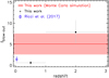 |
Fig. 19 Fraction of objects in the blow-out region (fblow–out) as a function of redshift. The blue square denotes the hard-X-ray-selected AGN sample (Ricci et al. 2017), while the black points are our eFEDS–W4-X sample. The red line and shaded region represent fblow–out calculated from the Monte Carlo simulation. |
5 Summary
In this work, we have investigated the physical properties of MIR galaxies at z < 4. The parent sample is drawn from 7780 WISE 22 μm (W4)-detected sources (the eFEDS–W4 sample) in the eFEDS catalog within a region of 140 deg2. By cross-matching the sample with the eFEDS main X-ray catalog, we find that 692 MIR galaxies (the eFEDS–W4-X sample) are detected and 7088 sources (the eFEDS–W4-nonX sample) are undetected by eROSITA. We compiled multiwavelength data from X-ray to FIR wavelengths and performed SED fitting with X-CIGALE. We performed X-ray spectral analysis for the eFEDS-W4 sample and X-ray stacking analysis for the eFEDS–W4-nonX sample. This multiwavelength approach provides AGN and host properties (such as the stellar mass, SFR, and NH) for the eFEDS–W4 galaxies.
Because of the wide-area data from eFEDS, we are able to determine various physical properties for the sample objects and find candidates of spatially rare populations such as ELIRGs. With all the caveats discussed in Sect. 4.3 in mind, the distribution of the eFEDS–W4 sample on the λEdd−NH plane, and a comparison with the output from a galaxy-merger simulation, indicate that approximately 5.0% of the sources in our sample are likely to be in a relatively short-lived (~30 Myr) feedback phase, in which nuclear material is blown out owing to radiation pressure from the AGN. The eROSITA all-sky survey (eRASS) is ongoing and is planned to continue until the end of 2023. Because eROSITA on SRG observes the entire sky in six months and will scan the entire sky eight times by the end of the mission, depth of the survey will increase progressively. The completion of eRASS (eRASS8) will thus provide a complete census of MIR galaxies over a wide luminosity and redshift range from the X-ray point of view. In that sense, this work establishes a benchmark for obtaining a full picture of such IR populations.
Acknowledgements
We thank the anonymous referee for the insightful comments and suggestions that improved the paper. We gratefully acknowledge Dr. Andy Goulding for useful discussion and comments, We also thank Dr. Claudio Ricci for helping to make Fig. 18. This work is based on data from eROSITA, the primary instrument aboard SRG, a joint Russian-German science mission supported by the Russian Space Agency (Roskosmos), in the interests of the Russian Academy of Sciences represented by its Space Research Institute (IKI), and the Deutsches Zentrum für Luft- und Raumfahrt (DLR). The SRG spacecraft was built by Lavochkin Association (NPOL) and its subcontractors, and is operated by NPOL with support from the Max-Planck Institute for Extraterrestrial Physics (MPE). The development and construction of the eROSITA X-ray instrument was led by MPE, with contributions from the Dr. Karl Remeis Observatory Bamberg & ECAP (FAU Erlangen-Nuernberg), the University of Hamburg Observatory, the Leibniz Institute for Astrophysics Potsdam (AIP), and the Institute for Astronomy and Astrophysics of the University of Tübingen, with the support of DLR and the Max Planck Society. The Argelander Institute for Astronomy of the University of Bonn and the Ludwig Maximilians Universität Munich also participated in the science preparation for eROSITA. The eROSITA data shown here were processed using the eSASS/NRTA software system developed by the German eROSITA consortium. The Hyper Suprime-Cam (HSC) collaboration includes the astronomical communities of Japan and Taiwan, and Princeton University. The HSC instrumentation and software were developed by the National Astronomical Observatory of Japan (NAOJ), the Kavli Institute for the Physics and Mathematics of the Universe (Kavli IPMU), the University of Tokyo, the High Energy Accelerator Research Organization (KEK), the Academia Sinica Institute for Astronomy and Astrophysics in Taiwan (ASIAA), and Princeton University. Funding was contributed by the FIRST program from the Japanese Cabinet Office, the Ministry of Education, Culture, Sports, Science and Technology (MEXT), the Japan Society for the Promotion of Science (JSPS), Japan Science and Technology Agency (JST), the Toray Science Foundation, NAOJ, Kavli IPMU, KEK, ASIAA, and Princeton University. This paper makes use of software developed for the Large Synoptic Survey Telescope. We thank the LSST Project for making their code available as free software at http://dm.lsst.org. This paper is based (in part) on data collected at the Subaru Telescope and retrieved from the HSC data archive system, which is operated by Subaru Telescope and Astronomy Data Center (ADC) at NAOJ. Data analysis was in part carried out with the cooperation of Center for Computational Astrophysics (CfCA), NAOJ. The Pan-STARRS1 Surveys (PS1) and the PS1 public science archive have been made possible through contributions by the Institute for Astronomy, the University of Hawaii, the Pan-STARRS Project Office, the Max Planck Society and its participating institutes, the Max Planck Institute for Astronomy, Heidelberg, and the Max Planck Institute for Extraterrestrial Physics, Garching, The Johns Hopkins University, Durham University, the University of Edinburgh, the Queen’s University Belfast, the Harvard-Smithsonian Center for Astrophysics, the Las Cumbres Observatory Global Telescope Network Incorporated, the National Central University of Taiwan, the Space Telescope Science Institute, the National Aeronautics and Space Administration under grant No. NNX08AR22G issued through the Planetary Science Division of the NASA Science Mission Directorate, the National Science Foundation grant No. AST-1238877, the University of Maryland, Eotvos Lorand University (ELTE), the Los Alamos National Laboratory, and the Gordon and Betty Moore Foundation. The Legacy Surveys consist of three individual and complementary projects: the Dark Energy Camera Legacy Survey (DECaLS; Proposal ID #2014B-0404; PIs: David Schlegel and Arjun Dey), the Beijing-Arizona Sky Survey (BASS; NOAO Prop. ID #2015A-0801; PIs: Zhou Xu and Xiaohui Fan), and the Mayall z-band Legacy Survey (MzLS; Prop. ID #2016A-0453; PI: Arjun Dey). DECaLS, BASS and MzLS together include data obtained, respectively, at the Blanco telescope, Cerro Tololo Inter-American Observatory, NSF’s NOIRLab; the Bok telescope, Steward Observatory, University of Arizona; and the Mayall telescope, Kitt Peak National Observatory, NOIRLab. The Legacy Surveys project is honored to be permitted to conduct astronomical research on Iolkam Du’ag (Kitt Peak), a mountain with particular significance to the Tohono O’odham Nation. NOIRLab is operated by the Association of Universities for Research in Astronomy (AURA) under a cooperative agreement with the National Science Foundation. This project used data obtained with the Dark Energy Camera (DECam), which was constructed by the Dark Energy Survey (DES) collaboration. Funding for the DES Projects has been provided by the U.S. Department of Energy, the U.S. National Science Foundation, the Ministry of Science and Education of Spain, the Science and Technology Facilities Council of the United Kingdom, the Higher Education Funding Council for England, the National Center for Supercomputing Applications at the University of Illinois at Urbana-Champaign, the Kavli Institute of Cosmological Physics at the University of Chicago, Center for Cosmology and Astro-Particle Physics at the Ohio State University, the Mitchell Institute for Fundamental Physics and Astronomy at Texas A&M University, Financiadora de Estudos e Projetos, Fundacao Carlos Chagas Filho de Amparo, Financiadora de Estudos e Projetos, Fundacao Carlos Chagas Filho de Amparo a Pesquisa do Estado do Rio de Janeiro, Conselho Nacional de Desenvolvimento Cientifico e Tecnologico and the Ministerio da Ciencia, Tecnologia e Inovacao, the Deutsche Forschungsgemeinschaft and the Collaborating Institutions in the Dark Energy Survey. The Collaborating Institutions are Argonne National Laboratory, the University of California at Santa Cruz, the University of Cambridge, Centro de Investigaciones Energeticas, Medioambientales y Tecnologicas-Madrid, the University of Chicago, University College London, the DES-Brazil Consortium, the University of Edinburgh, the Eidgenossische Technische Hochschule (ETH) Zurich, Fermi National Accelerator Laboratory, the University of Illinois at Urbana-Champaign, the Institut de Ciencies de l’Espai (IEEC/CSIC), the Institut de Fisica d’Altes Energies, Lawrence Berkeley National Laboratory, the Ludwig Maximilians Universitat Munchen and the associated Excellence Cluster Universe, the University of Michigan, NSF’s NOIRLab, the University of Nottingham, the Ohio State University, the University of Pennsylvania, the University of Portsmouth, SLAC National Accelerator Laboratory, Stanford University, the University of Sussex, and Texas A&M University. BASS is a key project of the Telescope Access Program (TAP), which has been funded by the National Astronomical Observatories of China, the Chinese Academy of Sciences (the Strategic Priority Research Program “The Emergence of Cosmological Structures” Grant # XDB09000000), and the Special Fund for Astronomy from the Ministry of Finance. The BASS is also supported by the External Cooperation Program of Chinese Academy of Sciences (Grant # 114A11KYSB20160057), and Chinese National Natural Science Foundation (Grant # 11433005). The Legacy Survey team makes use of data products from the Near-Earth Object Wide-field Infrared Survey Explorer (NEOWISE), which is a project of the Jet Propulsion Laboratory/California Institute of Technology. NEOWISE is funded by the National Aeronautics and Space Administration. The Legacy Surveys imaging of the DESI footprint is supported by the Director, Office of Science, Office of High Energy Physics of the U.S. Department of Energy under Contract No. DE-AC02-05CH1123, by the National Energy Research Scientific Computing Center, a DOE Office of Science User Facility under the same contract; and by the U.S. National Science Foundation, Division of Astronomical Sciences under Contract No. AST-0950945 to NOAO. Based on observations made with ESO Telescopes at the La Silla Paranal Observatory under programme IDs 177.A-3016, 177.A-3017, 177.A-3018 and 179.A-2004, and on data products produced by the KiDS consortium. The KiDS production team acknowledges support from: Deutsche Forschungsgemeinschaft, ERC, NOVA and NWO-M grants; Target; the University of Padova, and the University Federico II (Naples). Funding for the Sloan Digital Sky Survey IV has been provided by the Alfred P. Sloan Foundation, the U.S. Department of Energy Office of Science, and the Participating Institutions. SDSS-IV acknowledges support and resources from the Center for High Performance Computing at the University of Utah. The SDSS website is www.sdss.org. SDSS-IV is managed by the Astrophysical Research Consortium for the Participating Institutions of the SDSS Collaboration including the Brazilian Participation Group, the Carnegie Institution for Science, Carnegie Mellon University, Center for Astrophysics, Harvard & Smithsonian, the Chilean Participation Group, the French Participation Group, Instituto de Astrofisica de Canarias, The Johns Hopkins University, Kavli Institute for the Physics and Mathematics of the Universe (IPMU)/University of Tokyo, the Korean Participation Group, Lawrence Berkeley National Laboratory, Leibniz Institut für Astrophysik Potsdam (AIP), Max-Planck-Institut für Astronomie (MPIA Heidelberg), Max-Planck-Institut für Astrophysik (MPA Garching), Max-Planck-Institut für Extraterrestrische Physik (MPE), National Astronomical Observatories of China, New Mexico State University, New York University, University of Notre Dame, Observatário Nacional / MCTI, The Ohio State University, Pennsylvania State University, Shanghai Astronomical Observatory, United Kingdom Participation Group, Universidad Nacional Autόnoma de México, University of Arizona, University of Colorado Boulder, University of Oxford, University of Portsmouth, University of Utah, University of Virginia, University of Washington, University of Wisconsin, Vanderbilt University, and Yale University. The Herschel-ATLAS is a project with Herschel, which is an ESA space observatory with science instruments provided by European-led Principal Investigator consortia and with important participation from NASA. The H-ATLAS website is http://www.h-atlas.org/. This research is based on observations with AKARI, a JAXA project with the participation of ESA. Numerical computations/simulations were carried out (in part) using the SuMIRe cluster operated by the Extragalactic OIR group at ASIAA. This work is supported by JSPS KAKENHI grant Nos. 18J01050, 19K14759, and 19KK0076 (Y. Toba), 20H01946 (Y. Ueda), 20H01949 (T. Nagao), and 20K04014 (Y. Terashima).
References
- Ahumada, R., Allende Prieto, C., Almeida, A., et al. 2020, ApJS, 249, 3 [NASA ADS] [CrossRef] [Google Scholar]
- Aihara, H., Arimoto, N., Armstrong, R., et al. 2018a, PASJ, 70, S4 [NASA ADS] [Google Scholar]
- Aihara, H., Armstrong, R., Bickerton, S., et al. 2018b, PASJ, 70, S8 [NASA ADS] [Google Scholar]
- Aihara, H., AlSayyad, Y., Ando, M., et al. 2019, PASJ, 71, 114 [Google Scholar]
- Arnaboldi, M., Neeser, M. J., Parker, L. C., et al. 2007, The Messenger, 127, 28 [NASA ADS] [Google Scholar]
- Asmus, D., Gandhi, P., Hönig, S. F., Smette, A., & Duschl, W. J. 2015, MNRAS, 454, 766 [NASA ADS] [CrossRef] [Google Scholar]
- Assef, R. J., Stern, D., Noirot, G., et al. 2018, ApJS, 234, 23 [Google Scholar]
- Baes, M., Verstappen, J., de Looze, I., et al. 2011, ApJS, 196, 22 [NASA ADS] [CrossRef] [Google Scholar]
- Baldry, I. K., Liske, J., Brown, M. J. I., et al. 2018, MNRAS, 474, 3875 [Google Scholar]
- Barger, A. J., Cowie, L. L., Mushotzky, R. F., et al. 2005, AJ, 129, 578 [NASA ADS] [CrossRef] [Google Scholar]
- Bianchi, L., Shiao, B., & Thilker, D. 2017, ApJS, 230, 24 [Google Scholar]
- Birrer, S., & Amara, A. 2018, Phys. Dark Univ., 22, 189 [Google Scholar]
- Birrer, S., Amara, A., & Refregier, A. 2015, ApJ, 813, 102 [Google Scholar]
- Bongiorno, A., Merloni, A., Brusa, M., et al. 2012, MNRAS, 427, 3103 [Google Scholar]
- Boquien, M., Buat, V., & Perret, V. 2014, A&A, 571, A72 [NASA ADS] [CrossRef] [EDP Sciences] [Google Scholar]
- Boquien, M., Kennicutt, R., Calzetti, D., et al. 2016, A&A, 591, A6 [NASA ADS] [CrossRef] [EDP Sciences] [Google Scholar]
- Boquien, M., Burgarella, D., Roehlly, Y., et al. 2019, A&A, 622, A103 [NASA ADS] [CrossRef] [EDP Sciences] [Google Scholar]
- Bosch, J., Armstrong, R., Bickerton, S., et al. 2018, PASJ, 70, S5 [Google Scholar]
- Bourne, N., Dunne, L., Maddox, S. J., et al. 2016, MNRAS, 462, 1714 [NASA ADS] [CrossRef] [Google Scholar]
- Brand, K., Dey, A., Weedman, D., et al. 2006, ApJ, 644, 143 [NASA ADS] [CrossRef] [Google Scholar]
- Brunner, H., Liu, T., Lamer, G., et al. 2022, A&A, 661, A1 (eROSITA EDR SI) [NASA ADS] [CrossRef] [EDP Sciences] [Google Scholar]
- Brusa, M., Urrutia, T., Toba, Y., et al. 2022, A&A, 661, A9 (eROSITA EDR SI) [NASA ADS] [CrossRef] [EDP Sciences] [Google Scholar]
- Bruzual, G., & Charlot, S. 2003, MNRAS, 344, 1000 [NASA ADS] [CrossRef] [Google Scholar]
- Buat, V., Oi, N., Heinis, S., et al. 2015, A&A, 577, A141 [NASA ADS] [CrossRef] [EDP Sciences] [Google Scholar]
- Buchner, J., 2019, PASP, 131, 108005 [Google Scholar]
- Buchner, J., Georgakakis, A., Nandra, K., et al. 2014, A&A, 564, A125 [NASA ADS] [CrossRef] [EDP Sciences] [Google Scholar]
- Burgarella, D., Buat, V., & Iglesias-Páramo, J. 2005, MNRAS, 360, 1413 [NASA ADS] [CrossRef] [Google Scholar]
- Calderone, G., Nicastro, L., Ghisellini, G., et al. 2017, MNRAS, 472, 4051 [Google Scholar]
- Calzetti, D. 1997, AIP Conf. Ser., 408, 403 [NASA ADS] [CrossRef] [Google Scholar]
- Calzetti, D., Armus, L., Bohlin, R. C., et al. 2000, ApJ, 533, 682 [NASA ADS] [CrossRef] [Google Scholar]
- Carroll, C. M., Hickox, R. C., Masini, A. C., et al. 2021, ApJ, 908, 185 [NASA ADS] [CrossRef] [Google Scholar]
- Camps, P., & Baes, M. 2015, A&C, 9, 20 [NASA ADS] [Google Scholar]
- Chabrier, G. 2003, PASP, 115, 763 [Google Scholar]
- Chary, R., Casertano, S., Dickinson, M. E., et al. 2004, ApJS, 154, 80 [NASA ADS] [CrossRef] [Google Scholar]
- Chen, C.-T. J., Hickox, R. C., Goulding, A. D., et al. 2017, ApJ, 837, 145 [Google Scholar]
- Chen, X., Akiyama, M., Ichikawa, K., et al. 2020, ApJ, 900, 51 [NASA ADS] [CrossRef] [Google Scholar]
- Ciesla, L., Charmandaris, V., Georgakakis, A., et al. 2015, A&A, 576, A10 [NASA ADS] [CrossRef] [EDP Sciences] [Google Scholar]
- Ciesla, L., Boselli, A., Elbaz, D., et al. 2016, A&A, 585, A43 [NASA ADS] [CrossRef] [EDP Sciences] [Google Scholar]
- Corral, A., Georgantopoulos, I., Comastri, A., et al. 2016, A&A, 592, A109 [NASA ADS] [CrossRef] [EDP Sciences] [Google Scholar]
- Coupon, J., Czakon, N., Bosch, J., et al. 2018, PASJ, 70, S7 [Google Scholar]
- Croom, S. M., Richards, G. T., Shanks, T., et al. 2009, MNRAS, 392, 19 [CrossRef] [Google Scholar]
- Cui, X. Q., Zhao, Y. H., Chu, Y. Q., et al. 2012, Res. Astron. Astrophys., 12, 1197 [Google Scholar]
- Daddi, E., Alexander, D. M., Dickinson, M., et al. 2007, ApJ, 670, 173 [NASA ADS] [CrossRef] [Google Scholar]
- Dale, D. A., Helou, G., Magdis, G. E., et al. 2014, ApJ, 784, 11 [NASA ADS] [CrossRef] [Google Scholar]
- de Jong, J. T. A., Verdoes Kleijn, G. A., Kuijken, K. H., & Valentijn, E. A. 2013, Exp. Astron., 35, 25 [Google Scholar]
- Dey, A., Soifer, B. T., Desai, V., et al. 2008, ApJ, 677, 943 [NASA ADS] [CrossRef] [Google Scholar]
- Dey, A., Schlegel, D. J., Lang, D., et al. 2019, AJ, 157, 168 [Google Scholar]
- Ding, X., Silverman, J., Treu, T., et al. 2020, ApJ, 888, 37 [NASA ADS] [CrossRef] [Google Scholar]
- Donley, J. L., Rieke, G. H., Pérez-González, P. G., & Barro, G. 2008, ApJ, 687, 111 [NASA ADS] [CrossRef] [Google Scholar]
- Drinkwater, M. J., Jurek, R. J., Blake, C., et al. 2010, MNRAS, 401, 1429 [CrossRef] [Google Scholar]
- Driver, S. P., Hill, D. T., Kelvin, L. S., et al. 2011, MNRAS, 413, 971 [Google Scholar]
- Dullemond, C. P., Juhasz, A., Pohl, A., et al. 2012, Astrophysics Source Code Library [record ascl:1202.015] [Google Scholar]
- Eales, S., Dunne, L., Clements, D., et al. 2010, PASP, 122, 499 [NASA ADS] [CrossRef] [Google Scholar]
- Eckart, M. E., McGreer, I. D., Stern, D., Harrison, F. A., & Helfand, D. J. 2010, ApJ, 708, 584 [NASA ADS] [CrossRef] [Google Scholar]
- Edge, A., Sutherland, W., Kuijken, K., et al. 2013, The Messenger, 154, 32 [NASA ADS] [Google Scholar]
- Eisenhardt, P. R. M., Wu, J., Tsai, C.-W., et al. 2012, ApJ, 755, 173 [Google Scholar]
- Fabian, A. C., Celotti, A., & Erlund, M. C. 2006, MNRAS, 373, L16 [NASA ADS] [Google Scholar]
- Fabian, A. C., Vasudevan, R. V., Mushotzky, R. F., et al. 2009, MNRAS, 394, L89 [NASA ADS] [CrossRef] [Google Scholar]
- Fiore, F., Grazian, A., Santini, P., et al. 2008, ApJ, 672, 94 [NASA ADS] [CrossRef] [Google Scholar]
- Fiore, F., Puccetti, S., Brusa, M., et al. 2009, ApJ, 693, 447 [NASA ADS] [CrossRef] [Google Scholar]
- Foreman-Mackey, D., Hogg, D. W., Lang, D., & Goodman, J. 2013, PASP, 125, 306 [Google Scholar]
- Furusawa, H., Koike, M., Takata, T., et al. 2018, PASJ, 70, S3 [Google Scholar]
- Gaia Collaboration (Brown, A. G. A., et al.) 2018, A&A, 616, A1 [NASA ADS] [CrossRef] [EDP Sciences] [Google Scholar]
- Gandhi, P., Horst, H., Smette, A., et al. 2009, A&A, 502, 457 [NASA ADS] [CrossRef] [EDP Sciences] [Google Scholar]
- Goto, T., Arnouts, S., Inami, H., et al. 2011, MNRAS, 410, 573 [NASA ADS] [CrossRef] [Google Scholar]
- Griffin, M. J., Abergel, A., Abreu, A., et al. 2010, A&A, 518, L3 [EDP Sciences] [Google Scholar]
- Hasinger, G. 2008, A&A, 490, 905 [NASA ADS] [CrossRef] [EDP Sciences] [Google Scholar]
- Hewett, P. C., Warren, S. J., Leggett, S. K., & Hodgkin, S. T. 2006, MNRAS, 367, 454 [Google Scholar]
- Hickox, R. C., & Alexander, D. M. 2018, ARA&A, 56, 625 [Google Scholar]
- HI4PI Collaboration (Ben Bekhti, N., et al.) 2016, A&A, 594, A116 [NASA ADS] [CrossRef] [EDP Sciences] [Google Scholar]
- Huchra, J., Macri, L., Masters, K., et al. 2012, ApJS, 199, 26 [Google Scholar]
- Huang, S., Leauthaud, A., Murata, R., et al. 2018, PASJ, 70, S6 [CrossRef] [Google Scholar]
- Ichikawa, K., Ricci, C., Ueda, Y., et al. 2017, ApJ, 835, 74 [NASA ADS] [CrossRef] [Google Scholar]
- Ichikawa, K., Ricci, C., Ueda, Y., et al. 2019, ApJ, 870, 31 [NASA ADS] [CrossRef] [Google Scholar]
- Ilbert, O., Arnouts, S., McCracken, H. J., et al. 2006, A&A, 457, 841 [NASA ADS] [CrossRef] [EDP Sciences] [Google Scholar]
- Imanishi, M., Ichikawa, K., Takeuchi, T., et al. 2011, PASJ, 63, 447 [NASA ADS] [Google Scholar]
- Inoue, A. K. 2011, MNRAS, 415, 2920 [NASA ADS] [CrossRef] [Google Scholar]
- Ishibashi, W., Fabian, A. C., Ricci, C., et al. 2018, MNRAS, 479, 3335 [CrossRef] [Google Scholar]
- Jones, D. H., Saunders, W., Colless, M., et al. 2004, MNRAS, 355, 747 [NASA ADS] [CrossRef] [Google Scholar]
- Jones, D. H., Read, M. A., Saunders, W., et al. 2009, MNRAS, 399, 683 [Google Scholar]
- Jun, H. D., Assef, R. J., Carroll, C. M., et al. 2021, ApJ, 906, 21 [Google Scholar]
- Just, D. W., Brandt, W. N., Shemmer, O., et al. 2007, ApJ, 665, 1004 [Google Scholar]
- Kawada, M., Baba, H., Barthel, P. D., et al. 2007, PASJ, 59, 389 [Google Scholar]
- Kawanomoto, S., Uraguchi, F., Komiyama, Y., et al. 2018, PASJ, 70, 66 [Google Scholar]
- Kelly, B. C. 2007, ApJ, 665, 1489 [Google Scholar]
- Kennedy, J., & Eberhart, R. 1995, in Proceedings of ICNN’95 - International Conference on Neural Networks, 4, 1942 [CrossRef] [Google Scholar]
- Kessler, M. F., Steinz, J. A., Anderegg, M. E., et al. 1996, A&A, 500, 493 [Google Scholar]
- Komiyama, Y., Obuchi, Y., Nakaya, H., et al. 2018, PASJ, 70, S2 [Google Scholar]
- Kuijken, K., Heymans, C., Dvornik, A., et al. 2019, A&A, 625, A2 [NASA ADS] [CrossRef] [EDP Sciences] [Google Scholar]
- Lagache, G., Puget, J.-L., & Dole, H. 2005, ARA&A, 43, 727 [NASA ADS] [CrossRef] [Google Scholar]
- LaMassa, S. M., Georgakakis, A., Vivek, M., et al. 2019, AJ, 876, 50 [NASA ADS] [CrossRef] [Google Scholar]
- Lawrence, A., Warren, S. J., Almaini, O., et al. 2007, MNRAS, 379, 1599 [Google Scholar]
- Lang, D. 2014, AJ, 147, 108 [Google Scholar]
- Lang, D., Hogg, D. W., & Schlegel, D. J. 2016, AJ, 151, 36 [Google Scholar]
- Lanzuisi, G., Piconcelli, E., Fiore, F., et al. 2009, A&A, 498, 67 [NASA ADS] [CrossRef] [EDP Sciences] [Google Scholar]
- Le Floc’h, E., Aussel, H., Ilbert, O., et al. 2009, ApJ, 703, 222 [Google Scholar]
- Leitherer, C., Li, I.-H., Calzetti, D., & Heckman, T. M. 2002, ApJS, 140, 303 [Google Scholar]
- Li, J., Silverman, J. D., Ding, X., et al. 2021, ApJ, 918, 22 [NASA ADS] [CrossRef] [Google Scholar]
- Liu, T., Buchner, J., Nandra, K., et al., 2022, A&A, 661, A5 (eROSITA EDR SI) [NASA ADS] [CrossRef] [EDP Sciences] [Google Scholar]
- Lo Faro, B., Buat, V., Roehlly, Y., et al. 2017, MNRAS, 472, 1372 [NASA ADS] [CrossRef] [Google Scholar]
- Lupton, R. H., Gunn, J. E., & Szalay, A. S., 1999, AJ, 118, 3 [Google Scholar]
- Lyke, B. W., Higley, A. N., McLane, J. N., et al. 2020, ApJS, 250, 8 [NASA ADS] [CrossRef] [Google Scholar]
- Lyu, J., Rieke, G. H., & Shi, Y. 2017, ApJ, 835, 257 [NASA ADS] [CrossRef] [Google Scholar]
- Madau, P., & Dickinson, M. 2014, ARA&A, 52, 415 [Google Scholar]
- Magnelli, B., Elbaz, D., Chary, R. R., et al. 2011, A&A, 528, A35 [NASA ADS] [CrossRef] [EDP Sciences] [Google Scholar]
- Mainzer, A., Bauer, J., Cutri, R. M., et al. 2014, ApJ, 792, 30 [Google Scholar]
- Masoura, V. A., Mountrichas, G., Georgantopoulos, I., et al. 2018, A&A, 618, A31 [NASA ADS] [CrossRef] [EDP Sciences] [Google Scholar]
- Mateos, S., Carrera, F. J., Alonso-Herrero, A., et al. 2015, MNRAS, 449, 1422 [Google Scholar]
- Martin, D. C., Fanson, J., Schiminovich, D., et al. 2005, ApJ, 619, L1 [Google Scholar]
- Merloni, A., Bongiorno, A., Bolzonella, M., et al. 2010, ApJ, 708, 137 [Google Scholar]
- Merloni, A., Predehl, P., Becker, W., et al. 2012, ArXiv eprints [arXiv:1209.3114] [Google Scholar]
- Merloni, A., Bongiorno, A., Brusa, M., et al. 2014, MNRAS, 437, 3550 [Google Scholar]
- Merloni, A., Nandra, K., & Predehl, P. 2020, Nat. Astron., 4, 634 [Google Scholar]
- Miyazaki, S., Komiyama, Y., Kawanomoto, S., et al. 2018, PASJ, 70, S1 [NASA ADS] [Google Scholar]
- Mountrichas, G., Georgantopoulos, I., Ruiz, A., & Kampylis, G. 2020, MNRAS, 491, 1727 [NASA ADS] [CrossRef] [Google Scholar]
- Murakami, H., Baba, H., Barthel, P., et al. 2007, PASJ, 59, 369 [Google Scholar]
- Neugebauer, G., Habing, H. J., van Duinen, R., et al. 1984, ApJ, 278, L1 [NASA ADS] [CrossRef] [Google Scholar]
- Nishizawa, A. J., Hsieh, B., Tanaka, M., Takata, T., 2020, ArXiv eprints [arXiv:2003.01511] [Google Scholar]
- Noboriguchi, A., Nagao, T., Toba, Y., et al. 2019, ApJ, 876, 132 [NASA ADS] [CrossRef] [Google Scholar]
- Noll, S., Burgarella, D., Giovannoli, E., et al. 2009, A&A, 507, 3 [Google Scholar]
- Pavlinsky, M., Tkachenko, A., Levin, V., et al. 2021, A&A, 650, A42 [EDP Sciences] [Google Scholar]
- Petrosian, V. 1976, ApJ, 209, L1 [Google Scholar]
- Pilbratt, G. L., Riedinger, J. R., Passvogel, T., et al. 2010, A&A, 518, L1 [NASA ADS] [CrossRef] [EDP Sciences] [Google Scholar]
- Poglitsch, A., Waelkens, C., Geis, N., et al. 2010, A&A, 518, L2 [NASA ADS] [CrossRef] [EDP Sciences] [Google Scholar]
- Predehl, P., Andritschke, R., Arefiev, V., et al. 2021, A&A, 647, A1 [EDP Sciences] [Google Scholar]
- Rakshit, S., Stalin, C. S., & Kotilainen, J. 2020, ApJS, 249, 17 [Google Scholar]
- Ricci, C., Trakhtenbrot, B., Koss, M. J., et al. 2017, Nature, 549, 488 [NASA ADS] [CrossRef] [Google Scholar]
- Rowan-Robinson, M. 2000, MNRAS, 316, 885 [Google Scholar]
- Ruiz, A., Corral, A., Mountrichas, G., & Georgantopoulos, I. 2018, A&A, 618, A52 [NASA ADS] [CrossRef] [EDP Sciences] [Google Scholar]
- Saitoh, T. R., Daisaka, H., Kokubo, E., et al. 2008, PASJ, 60, 667 [NASA ADS] [Google Scholar]
- Saitoh, T. R., Daisaka, H., Kokubo, E., et al. 2009, PASJ, 61, 481 [NASA ADS] [Google Scholar]
- Salvato, M., Buchner, J., Budavári, T., et al. 2018, MNRAS, 473, 4937 [Google Scholar]
- Salvato, M., Wolf, J., Dwelly, T., et al. 2022, A&A, 661, A3 (eROSITA EDR SI) [NASA ADS] [CrossRef] [EDP Sciences] [Google Scholar]
- Sanders, D. B., & Mirabel, I. F. 1996, ARA&A, 34, 749 [Google Scholar]
- Sawicki, M. 2012, PASP, 124, 1208 [NASA ADS] [CrossRef] [Google Scholar]
- Shen, Y., Richards, G. T., Strauss, M. A., et al. 2011, ApJS, 194, 45 [Google Scholar]
- Skrutskie, M., Cutri, R., Stiening, R., et al. 2006, AJ, 131, 1163 [Google Scholar]
- Soifer, B. T., Helou, G., & Werner, M. 2008, ARA&A, 46, 201 [NASA ADS] [CrossRef] [Google Scholar]
- Stalevski, M., Fritz, J., Baes, M., Nakos, T., & Popovic, L. C. 2012, MNRAS, 420, 2756 [NASA ADS] [CrossRef] [Google Scholar]
- Stalevski M., Ricci C., Ueda Y., et al. 2016, MNRAS, 458, 2288 [NASA ADS] [CrossRef] [Google Scholar]
- Stemo, A., Comerford, J. M., Barrows, R. S., et al. 2020, ApJ, 888, 78 [NASA ADS] [CrossRef] [Google Scholar]
- Stern, D. 2015, ApJ, 807, 129 [Google Scholar]
- Suh, H., Civano, F., Trakhtenbrot, B., et al. 2020, ApJ, 889, 32 [NASA ADS] [CrossRef] [Google Scholar]
- Sutherland, W., & Saunders, W. 1992, MNRAS, 259, 413 [Google Scholar]
- Sunyaev, R., Arefiev, V., Babyshkin, V., et al. 2021, A&A, 656, A132 [NASA ADS] [CrossRef] [EDP Sciences] [Google Scholar]
- Toba, Y., & Nagao, T. 2016, ApJ, 820, 46 [Google Scholar]
- Toba, Y., Nagao, T., Strauss, M. A., et al. 2015, PASJ, 67, 86 [Google Scholar]
- Toba, Y., Nagao, T., Kajisawa, M., et al. 2017a, ApJ, 835, 36 [NASA ADS] [CrossRef] [Google Scholar]
- Toba, Y., Nagao, T., Wang, W.-H., et al. 2017b, ApJ, 840, 21 [NASA ADS] [CrossRef] [Google Scholar]
- Toba, Y., Bae, H.-J., Nagao, T., et al. 2017c, ApJ, 850, 140 [NASA ADS] [CrossRef] [Google Scholar]
- Toba, Y., Komugi, S., Nagao, T., et al. 2017d, ApJ, 851, 98 [NASA ADS] [CrossRef] [Google Scholar]
- Toba Y., Ueda J., Lim C.-F., et al. 2018, ApJ, 857, 31 [NASA ADS] [CrossRef] [Google Scholar]
- Toba, Y., Ueda, Y., Matsuoka, K., et al. 2019a, MNRAS, 484, 196 [Google Scholar]
- Toba, Y., Yamashita, T., Nagao, T., et al. 2019b, ApJS, 243, 15 [Google Scholar]
- Toba, Y., Yamada, S., Ueda, Y., et al. 2020a, ApJ, 888, 8 [Google Scholar]
- Toba, Y., Wang, W.-H., Nagao, T., et al. 2020b, ApJ, 889, 76 [Google Scholar]
- Toba, Y., Goto, T., Oi, N., et al. 2020c, ApJ, 899, 35 [Google Scholar]
- Toba, Y., Ueda, Y., Gandhi, P., et al. 2021a, ApJ, 912, 91 [NASA ADS] [CrossRef] [Google Scholar]
- Toba, Y., Brusa, M., Liu, T., et al. 2021b, A&A, 649, L11 [NASA ADS] [CrossRef] [EDP Sciences] [Google Scholar]
- Treister, E., Urry, C. M., Van Duyne, J., et al. 2006, ApJ, 640, 603 [NASA ADS] [CrossRef] [Google Scholar]
- Treister, E., Cardamone, C. N., Schawinski, K., et al. 2009, ApJ, 706, 535 [NASA ADS] [CrossRef] [Google Scholar]
- Trump, J. R., Impey, C. D., & Kelly, B. C. 2011, ApJ, 733, 60 [NASA ADS] [CrossRef] [Google Scholar]
- Tsai, C.-W., Eisenhardt, P. R. M., Wu, J., et al. 2015, ApJ, 805, 90 [Google Scholar]
- Ueda, Y., Akiyama, M., Hasinger, G., Miyaji, T., & Watson, M. G. 2014, ApJ, 786, 104 [Google Scholar]
- Valiante, E., Smith, M. W. L., Eales, S., et al. 2016, MNRAS, 462, 3146 [NASA ADS] [CrossRef] [Google Scholar]
- Veilleux, S., Sanders, D. B., & Kim, D.-C. 1999, ApJ, 522, 139 [NASA ADS] [CrossRef] [Google Scholar]
- Verner, D. A., Ferland, G. J., Korista, K. T., & Yakovlev, D. G. 1996, ApJ, 465, 487 [Google Scholar]
- Vestergaard, M., & Peterson, B. M. 2006, ApJ, 641, 689 [Google Scholar]
- Werner, M. W., Roellig, T. L., Low, F. J., et al. 2004, ApJS, 154, 1 [NASA ADS] [CrossRef] [Google Scholar]
- Wilms, J., Allen, A., & McCray, R. 2000, ApJ, 542, 914 [Google Scholar]
- Wright, E. L., Eisenhardt, P. R. M., Mainzer, A. K., et al. 2010, AJ, 140, 1868 [Google Scholar]
- Wu, J., Tsai, C.-W., Sayers, J., et al. 2012, ApJ, 756, 96 [Google Scholar]
- Yamamura, I., Makiuchi, S., Koga, T., AKARI Team, 2018, in The Cosmic Wheel and the Legacy of the AKARI Archive: From Galaxies and Stars to Planets and Life, eds. T. Ootsubo, I. Yamamura, K. Murata, & T. Onaka, 227 [Google Scholar]
- Yang, G., Boquien, M., Buat, V., et al. 2020, MNRAS, 491, 740 [Google Scholar]
- York, D. G., Adelman, J., Anderson, J. E., Jr. et al. 2000, AJ, 120, 1579 [NASA ADS] [CrossRef] [Google Scholar]
- Yutani, N., Toba, Y., & Wada, K., 2021, PASJ, submitted [Google Scholar]
The original definition of DOGs was f24 > 0.3 mJy and R–[24] > 14, where R and [24] represent Vega magnitudes in the R-band and at 24 μm, respectively (see Dey et al. 2008, for more detail).
We visually confirmed that there were no spurious detections at 22 μm based on W4 images.
Salvato et al. (2022) provided multiwavelength photometric data up to MIR for X-ray sources in the eFEDS main X-ray catalog. Nevertheless, we compiled data ourselves up to the far-IR (FIR) to perform SED analysis for the eFEDS-W4 sample regardless of eROSITA detections using identical photometry with UV-FIR (see Sect. 2.5).
zspec used in this work were obtained from the report by Salvato et al. (2022) except for a proprietary zspec, which was obtained through the SPectroscopic IDentification of ERosita Sources (SPIDERS)-SDSS-IV follow-up campaign (Merloni et al., in prep.).
A small bug was reported by the KiDS team, which induces incorrect photometry in some tiles; for these tiles, the data in DR4.1 should be replaced. However, we confirmed that the eFEDS sources were not located in the problematic tiles; therefore, we used the original DR4 catalog (see http://kids.strw.leidenuniv.nl/DR4/index.php).
X-CIGALE handles the SED fitting of photometric data with upper limits by employing the method presented by Sawicki (2012). This method computes χ2 by introducing the error function (see Eqs. (15) and (16)in Boquien et al. 2019).
Because the i-band data provide the highest image quality among the HSC five-band data for the typical seeing of 0″.6 (Aihara et al. 2018a), the i-band is ideal for 2D image analysis.
The values of NH and λEdd were estimated by Ricci et al. (2017) using X-ray and optical spectra. Hence, those values are well constrained compared with this work.
All Tables
Absorption-corrected X-ray luminosities in the 2–10 keV band of the stacked eFEDS–W4-nonX subsample.
All Figures
|
Fig. 1 Flowchart of the sample-selection process. |
| In the text | |
|
Fig. 2 Sky distribution of the 692 eFEDS–W4-X sample (black points) in the eFEDS catalog. The blue-shaded region represents the survey footprint of the HSC-SSP S19A, while the green and red outlines represent those of KiDS DR4 and H-ATLAS DR1, respectively. |
| In the text | |
|
Fig. 3 Redshift distribution of the eFEDS–W4-X subsample (blue) and the eFEDS-W4-non X sample (gray). Objects at z < 4 are used for the multiwavelength analysis. |
| In the text | |
|
Fig. 4 Examples of quasar-host decomposition based on the HSC i-band image. From left to right: (i) the observed HSC i-band image, (ii) the best-fit point source + host galaxy model, (iii) the data minus the point source model (the pure-galaxy image), (iv) fitting residuals divided by the variance map, and (v) one-dimensional surface brightness profiles (top) and the corresponding residuals (bottom). |
| In the text | |
|
Fig. 5 Comparison between zspec and zphoto for the eFEDS-W4-nonX sample. The red solid line represents zspec = zphoto. The red dotted lines denote Δz/(1+zspec) = ±0.15. The bottom panel shows Δz/(1+zspec) as a function of zspec. |
| In the text | |
|
Fig. 6 Examples of the X-ray spectra from eROSITA. The best-fit model and its 99% confidence interval are displayed as blue-shaded regions. For each source, the lower panel shows comparison of the data with the best-fit model in terms of (data–model)/error, where error is calculated as the square root of the model predicted number of counts. |
| In the text | |
|
Fig. 7 Absorption-corrected X-ray luminosity in the 0.5–2 keV band for the 339 objects in the eFEDS–W4-X subsample as a function of redshift. |
| In the text | |
|
Fig. 8 Absorption-corrected X-ray luminosity in the 2–10 keV band for the 339 objects in the eFEDS–W4-X subsample as a function of redshift. The green stars represent the eFEDS–W4-nonX subsample used in the X-ray stacking analysis, for which we calculated LX by assuming NH = 0 cm−2 and Γ = 2.0. The yellow star denotes the ELIRG (WISEJ0909+0002) reported in Toba et al. (2021b). |
| In the text | |
|
Fig. 9 Histogram of hydrogen column density (NH) measured from the eROSITA X-ray spectra for 339 objects. |
| In the text | |
|
Fig. 10 Examples of SED fitting. The black points are photometric data, and the gray solid line represents the resulting best-fit SED. The inset shows the SED at 0.1–500 μm, with the contributions from the stellar, AGN, and SF components to the total SED shown as blue, yellow, and red lines, respectively. |
| In the text | |
|
Fig. 11 IR luminosity as a function of redshift. The green stars represent the eFEDS–W4-nonX subsample, for which the values of LIR are the mean and standard deviation for sources (indicated by green dots) in each redshift bin, as given in Table 2. The yellow star represent the ELIRG (WISEJ0909+0002) reported in Toba et al. (2021b). Objects with red circles have FIR detections from Herschel or AKARI. |
| In the text | |
|
Fig. 12 Differences in E(B − V),, the stellar mass (M*), the SFR, and LIR derived from X-CIGALE in this work and those derived from the mock catalog. (a) ΔΕ(Β − V),, (b) M*, (c) SFR, and (d) LIR as functions of redshift. Right-hand panels: histograms of each quantity. The red dotted lines correspond to Δ = 0. |
| In the text | |
|
Fig. 13 Stacked X-ray images (2′ × 2′) of the eFEDS–W4-nonX samples as a function of redshift bin. From left to right: bins are z < 0.1, 0.1 < z < 0.25, 0.25 < z < 0.5, 0.5 < z < 1.0, z > 1.0, and all the samples. The energy bands (in the observed frame) of the subsample are 0.2–10, 0.2–0.5, 0.6–2.3, and 2.3–5.0 keV from top to bottom. |
| In the text | |
|
Fig. 14 Composite SEDs of the eFEDS-W4-X subsample (blue) and eFEDS-W4-nonX subsample (red). The shaded regions represent the standard deviations of the stacked SED medians. There are no data points in the gray region, and composite SEDs are excluded. The inset displays a magnified view of the rest-frame optical-to-FIR SEDs. |
| In the text | |
|
Fig. 15 Relationship between the rest-frame 6 μm luminosity contributed by AGN and the absorption-corrected, rest-frame 2–10-keV luminosity for the eFEDS–W4 sample. The best-fit linear function in log–log space and its 1er dispersion are shown as the solid blue line and the shaded blue band, respectively. The cyan line represents the best-fit for an X-ray-selected AGN sample from the BUXS catalog (Mateos et al. 2015). The orange and magenta lines show two-dimensional polynomial and bilinear relations from Stern (2015) and Chen et al. (2017), respectively. The green stars represent the eFEDS–W4-nonX subsample used for the X-ray stacking analysis in which we obtained the weighted mean and standard deviation in each redshift bin by taking into account the uncertainties in NH (NH = 0–1023 cm−2). The black dotted line represents a one-to-one correspondence between the 6 μm and 2–10 keV luminosities. The yellow star denotes the ELIRG (WISEJ0909+0002) reported in Toba et al. (2021b). |
| In the text | |
|
Fig. 16 AGN fraction (LIR(AGN)/LIR) of the eFEDS–W4-X sample at 0.2 < z < 0.8 versus the point-source fraction of the i-band flux density |
| In the text | |
|
Fig. 17 Ratio of the stellar mass derived from SED fitting with all the data |
| In the text | |
|
Fig. 18 Relation between log NH and λEdd for the eFEDS–W4 sample. The yellow star represents the ELIRG (Toba et al. 2021b), and the orange square shows the location of XID439 (see text). Objects with red circles have optical spectra from SDSS DR16. Typical uncertainties in log NH and λEdd are shown at the bottom right. The dotted line denotes the effective Eddington limit ( |
| In the text | |
|
Fig. 19 Fraction of objects in the blow-out region (fblow–out) as a function of redshift. The blue square denotes the hard-X-ray-selected AGN sample (Ricci et al. 2017), while the black points are our eFEDS–W4-X sample. The red line and shaded region represent fblow–out calculated from the Monte Carlo simulation. |
| In the text | |
Current usage metrics show cumulative count of Article Views (full-text article views including HTML views, PDF and ePub downloads, according to the available data) and Abstracts Views on Vision4Press platform.
Data correspond to usage on the plateform after 2015. The current usage metrics is available 48-96 hours after online publication and is updated daily on week days.
Initial download of the metrics may take a while.