| Issue |
A&A
Volume 661, May 2022
The Early Data Release of eROSITA and Mikhail Pavlinsky ART-XC on the SRG mission
|
|
|---|---|---|
| Article Number | A37 | |
| Number of page(s) | 13 | |
| Section | Interstellar and circumstellar matter | |
| DOI | https://doi.org/10.1051/0004-6361/202141054 | |
| Published online | 18 May 2022 | |
First studies of the diffuse X-ray emission in the Large Magellanic Cloud with eROSITA
1
Dr. Karl Remeis Observatory, Erlangen Centre for Astroparticle Physics, Friedrich-Alexander-Universität Erlangen-Nürnberg,
Sternwartstraße 7,
96049
Bamberg,
Germany
e-mail: This email address is being protected from spambots. You need JavaScript enabled to view it.
2
Max-Planck-Institut für extraterrestrische Physik,
Giessenbachstrasse 1,
85748
Garching,
Germany
3
Argelander-Institut für Astronomie, Universität Bonn,
Auf dem Hugel 71,
53121
Bonn,
Germany
4
Ioffe Institute,
26 Politekhnicheskaya,
St Petersburg
194021,
Russia
5
Western Sydney University,
Locked Bag 1797,
Penrith South DC,
NSW 2751,
Australia
6
CSIRO Astronomy and Space Science,
PO Box 76,
Epping,
NSW 1710,
Australia
7
Cerro Tololo Inter-American Observatory/NSF’s NOIRLab,
Casilla 603,
La Serena,
Chile
8
International Centre for Radio Astronomy Research (ICRAR), M468, University of Western Australia,
Crawley,
WA
6009,
Australia
9
ARC Centre of Excellence for All Sky Astrophysics in 3 Dimensions (ASTRO 3D),
Australia
Received:
12
April
2021
Accepted:
7
July
2021
Abstract
Context. In the first months after its launch in July 2019, the extended Roentgen Survey with an Imaging Telescope Array (eROSITA) on board Spektrum-Roentgen-Gamma performed long-exposure observations in the regions around supernova (SN) 1987A and super-nova remnant (SNR) N132D in the Large Magellanic Cloud (LMC).
Aims. We analysed the distribution and the spectrum of the diffuse X-ray emission in the observed fields to determine the physical properties of the hot phase of the interstellar medium (ISM).
Methods. Spectral extraction regions were defined using the Voronoi tessellation method. The spectra were fit with a combination of thermal and non-thermal emission models. The eROSITA data are complemented by newly derived column density maps for the Milky Way and the LMC, 888 MHz radio continuum map from the Australian Square Kilometer Array Pathfinder, and optical images of the Magellanic Cloud Emission Line Survey.
Results. We detect significant emission from thermal plasma with kT = 0.2 keV in all the regions. There is also an additional higher- temperature emission component from a plasma with kT ≈ 0.7 keV. The surface brightness of this component is one order of magnitude lower than that of the lower-temperature component. In addition, non-thermal X-ray emission is significantly detected in the superbubble 30 Dor C. The absorbing column density NH in the LMC derived from the analysis of the X-ray spectra taken with eROSITA is consistent with the NH obtained from the emission of the cold medium over the entire area. Neon abundance is enhanced in the regions in and around 30 Dor and SN 1987A, indicating that the ISM has been chemically enriched by the young stellar population. In the centre of 30 Dor, there are two bright extended X-ray sources, which coincide with the stellar cluster RMC 136 and the Wolf-Rayet stars RMC 139 and RMC 140. For both regions the emission is best modelled with a high-temperature (kT > 1 keV) non-equilibrium ionisation plasma emission and a non-thermal component with a photon index of Γ = 1.3. In addition, we detect an extended X-ray source at the position of the optical SNR candidate J0529-7004 with thermal emission, and thus confirm its classification as an SNR.
Conclusions. Using data from the early observations of the regions around SN 1987A and SNR N132D with eROSITA we confirm that there is thermal interstellar plasma in the entire observed field. eROSITA with its large field of view and high sensitivity at lower X-ray energies allows us for the first time to carry out a detailed study of the ISM at high energies consistently over a large region in the LMC. We thus measure the properties of the interstellar plasma and the distribution of non-thermal particles and derive the column density of the cold matter on the line of sight.
Key words: Magellanic Clouds / X-rays: ISM / ISM: structure / ISM: bubbles / ISM: supernova remnants / ISM: abundances
© ESO 2022
1 Introduction
The Large Magellanic Cloud (LMC) is the largest satellite galaxy of the Milky Way at a distance of 50 kpc (e.g. de Grijs et al. 2014). It is a gas-rich dwarf galaxy with an almost face-on planar disk and many interesting asymmetric features, such as spiral arms, off-centre bar, and a shell-like structure (de Vaucouleurs 1955). Older stellar populations dominate the LMC mass and are either smoothly distributed in the disk or form a homogeneous stellar halo (Borissova et al. 2004, 2006). Young stars, on the contrary, are mainly found in the spiral arms (Youssoufi et al. 2019). The stellar populations indicate that the last major star formation in the Magellanic Clouds (MCs) occurred 200 ± 50 Myr ago (e.g. Joshi & Panchal 2019, and references therein).
Optical emission line and radio images reveal that the LMC has a large number of bright H II regions with a wide distribution in the disk. The most distinct object among them is the giant H II- region 30 Doradus (30 Dor), also called the Tarantula nebula. It is located north of the eastern end of the stellar bar of the LMC and is host to the massive super-star cluster RMC 136.
The distribution of cold gas as seen in H I emission (Mathewson et al. 1974; Kim et al. 2003) also reveals interesting structures in the eastern part of the LMC. As found by Luks & Rohlfs (1992), there are two distinct H I components in the LMC, the L- and D-components. The D-component covers most of the LMC and is located in the plane of the galaxy disk. The L-component on the other hand is much more localised and has radial velocities that are ~30-60 km s–1 lower than the D-component. The H I gas distribution suggests that there was a close encounter between the LMC and the Small Magellanic Cloud (SMC) about 150-200 Myr ago (Fujimoto & Noguchi 1990). Fukui et al. (2017) revisited the H I gas in the LMC and reported that the D- and L-components show a complementary distribution. They also found a third component, called the I-component, with radial velocities between the L-and D-component. The I-component was most likely formed by interactions between the two major components. In addition, Fukui et al. (2017) found a correlation between a large elongated complex of molecular clouds seen in CO called the CO ridge (Fukui et al. 1999; Mizuno et al. 2001; Fukui et al. 2008) and the likely interaction region. The CO ridge is located west of 30 Doradus and extends towards the south.
At high energies, the LMC is known to host bright supernova remnants (SNRs, e.g. N132D) and is a unique place where we can study the evolution of a supernova (SN) into an SNR (SN 1987A). South of 30 Dor, east of the CO ridge, a large diffuse structure called the X-ray spur was observed in X-rays in the ROSAT survey of the LMC (Blondiau et al. 1997; Points et al. 2001). The X-ray spur is located south of 30 Dor and the supergiant shell LMC 2 (LMC-SGS 2) and seems to coincide with the regions where the L- and D-components of H I collide with each other. The analysis of X-ray data taken with XMM-Newton has shown that the X-ray spur was most likely caused by the H I collision (Knies et al. 2021). While in 30 Dor and in regions around it the interstellar medium (ISM) was heated by the stellar winds and supernovae of massive stars, there is no indication of stellar heating in the X-ray spur.
In this paper we present the analysis of the diffuse X-ray emission around 30 Dor and SNR N132D in the LMC based on the first observations with the extended ROentgen survey with an Imaging Telescope Array (eROSITA; Merloni et al. 2012; Predehl et al. 2021), taken during the early commissioning and calibration phase of the mission. eROSITA is a new X-ray telescope, which was launched on July 13, 2019, on board the Spektrum-Roentgen-Gamma (Spektr-RG, SRG) spacecraft. eROSITA consists of seven telescope modules (TMs), each equipped with a CCD detector. With its large field of view (FOV) with a diameter of ~1 degree and high sensitivity in the energy band up to 10 keV, eROSITA allows us to study the distribution and the spectral properties of large extended X-ray emission for the first time. We supplement our study with the latest generation of radio survey data from the Australian Square Kilometer Array Pathfinder (ASKAP, Johnston et al. 2008; Hotan et al. 2021) and optical emission line images of the Magellanic Cloud Emission Line Survey (MCELS, Smith et al. 2004). The studies of the point sources in the same observations and of SN 1987A are presented in separate papers by Haberl et al. (2022) and Maitra et al. (2022), respectively. We report on the study of the diffuse X-ray emission in the entire LMC, which will be based on the eROSITA All-Sky Survey (eRASS) data in future publications.
2 Data
2.1 eROSITA
During the journey to Lagrange point L2, where SRG has been operating in a stable orbit ever since, commissioning tests and calibration of the instruments were carried out, along with performance verification observations. The first-light observation of eROSITA was pointed at SN 1987A next to 30 Dor, while several calibration observations were performed around SNR N132D. We used the data from eROSITA observations in the LMC obtained during the commissioning and calibration phases (see Table 1). The observations were carried out in the pointing or the field-scan mode and were roughly pointed at PSR J0540-6919, SN 1987A, and SNR N132D, some of them with offsets of 20′ for calibration purposes. The data were processed with the eROSITA Science Analysis Software System (eSASS, Brunner et al. 2022). The eSASS pre-processing pipeline produces energy calibrated event files, which can then be used for the analysis. For the Early Data Release (EDR) we used the data of the processing version c001.
2.2 NH map
X-rays interact via photoelectric absorption with baryonic matter distributed along the line of sight. The absorption cross section is a function of energy σ ∝ E–3 (Wilms et al. 2000), implying that the low-energy portion of the total X-ray spectrum is strongly affected by photoelectric absorption. Hydrogen and helium are the most abundant elements in space. Their abundance ratio is still very close to the value defined by the primordial nucleosynthesis. Because of hydrogen’s dominance in abundance, the number of atomic and molecular hydrogen is used as a proxy for the total number of interstellar and intergalactic gas atoms.
The amount of neutral atomic hydrogen can be measured via the H I 21cm line emission. Here, we make use of the HI4PI survey (HI4PI Collaboration 2016)1, which is based on the data of the Effelsberg-Bonn H I Survey (EBHIS, Winkel et al. 2016) and the third revision of the Galactic All-Sky Survey (GASS, Kalberla & Haud 2015). HI4PI quantifies the total H I hydrogen atoms within the velocity range of –600 ≤ vLSR[kms−1] ≤ 600, comprising the full radial velocity range covered by the Milky Way H I (Kalberla & Kerp 2009) and the Magellanic Cloud System (Brüns et al. 2005). The integrated HI4PI NHI map therefore displays a complex superposition of the H I emission of the Milky Way and that of the Magellanic Clouds; however, they populate very different radial velocity ranges. The emission in the Magellanic Clouds is found at 200 ≤ vLSR[kms−1] ≤ 350 (Kim et al. 2003), while the Milky Way’s H I emission is around vLSR[kms−1] ≃ 0 (see Fig. 1; Brüns et al. 2005). We split up the H I data into these two velocity regimes.
Observations of the 21 cm line do not take into account hydrogen nuclei in molecular phase. Therefore, NHI is only a lower limit to the true amount of hydrogen nuclei causing the soft X-ray absorption. To identify regions with significant amounts of molecular hydrogen we search for deviations from the median of the field-averaged gas-to-dust ratio NHI/AV. Neither the number of dust grains nor the number of hydrogen nuclei is modified during a phase transition from H I to H2, but the NHI/AV. ratio is. Regions with significantly low values for NHI/AV. spatially mark molecular gas.
With the aim of getting a reliable estimate of the foreground NH;Gal, because it modifies the soft X-ray emission from the LMC by photoelectric absorption, we cross-correlated the HI4PI data with the interstellar reddening EB−V data from Schlegel et al. (1998). We applied the correction EB−V(true) = 0.884 • EB−V (Schlafly & Finkbeiner 2011). According to Cardelli et al. (1989) and Weingartner & Draine (2001) the visual extinction of the diffuse interstellar medium is AV = 3.1EB−V, which is adopted in the following. We evaluated NHI/AV across an area of about 8000 deg2, which is sufficiently large to distinguish between the Magellanic Cloud System and the Milky Way halo gas. For the Milky Way gas we find a value of NHI/AV = (2.04 ± 0.15) × 1021 cm−2 mag−1, which is compatible with Güver & Özel (2009) who determined (2.21 ± 0.09) x 1021 cm−2 mag−1. To obtain a map of the distribution of the excess extinction regions, we calculated the mean NHI/AV for the Milky Way halo gas by applying a spatial mask to exclude the H I emission of the Magellanic Cloud System. Excess extinction regions, which deviate significantly from the field-averaged median value, are shown by the contour lines in Fig. 2. While the H I data allow us to distinguish between the Milky Way and the Magellanic Cloud System emission, it is not possible to separate the optical extinction data. We do not find any evidence for additional neutral large-scale structures in the immediate vicinity of our field observed with eROSITA, indicating that there are no significant amounts of molecular gas in the Milky Way Galaxy in this area of the sky. The LMC X-ray radiation is dominantly modulated only by its intrinsic H I distribution (see Sect. 6.4). On smaller angular scales additional soft X-ray shadows are expected because of the three dimensional structure of neutral and molecular interstellar medium that belongs to the LMC itself.
Used eROSITA observations.
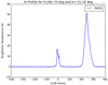 |
Fig. 1 H I velocity profile at an example position in the LMC (RA = 85.75°, Dec = -70.20°) |
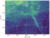 |
Fig. 2 Spatial distribution the Milky Way’s NHI column density for VLSR = −155 to +80 kms−1 above a threshold of NHI = 3 x 1019 cm−2 with a maximum of 1 x 1021 cm−2. Superimposed as contours is the spatial distribution of the Milky Way gas with excess optical extinction derived from the NHI/AV ratio (see text for details). The contours correspond to NH2 = 5 × 1019 cm−2 and to 1, 2, and 3 x 1020 cm−2. The LMC is located at l = 280°, b = -33°; the SMC at l = 302°, b = −44°. The yellow ellipse indicates the area observed with eROSITA. |
3 X-ray analysis
3.1 Images
eROSITA data were analysed using the eSASS version eSASSusers_201009. We created exposure-corrected mosaic images using the data in the broad band of 0.2–10.0 keV and in the following sub-bands: 0.2–0.5 keV, 0.5–1.0 keV, 1.0–2.0 keV, and 2.0–10.0 keV. To create the images, event files for all seven telescope modules (TMs) of eROSITA were binned with a bin size of 160 pixels, yielding counts images with a pixel size of 8″. These counts images and corresponding exposure maps were created for each observation and energy band. After combining the images and exposure maps into large mosaics of all observations, the mosaics of the counts images were divided by the respective exposure-map mosaics to create exposure-corrected mosaic images. Figure 3 shows the mosaic images of all data in Table 1 below 2.0 keV and an exposure map of all observations in the broad band of 0.2−10.0 keV. To create the mosaic images we applied a lower cut for the exposure of 1σ below the mean value to mask out the outer areas of the FOVs in which the photon statistics were low.
In Wolter Type-I telescopes like eROSITA, single reflections of photons from nearby X-ray sources outside the FOV on the second hyperboloid mirror shells can also reach the detectors. Even though baffles in front of the telescopes can reduce the effect, it will result in stray light in the data and contaminate both the images and the spectra. In our case single reflections from photons from SNR N132D can become significant in observations to the east. We therefore carefully inspected the images for possible stray light, which would have been visible as an enhanced arc-like structure in one-half of the FOV of each observation on the side close to N132D. Fortunately, it caused no visible effect in the images. For the spectral analysis, for which we used the data of observations 700 156, 700 161, and 700 179, any contamination by additional emission from N132D will only be visible in the spectra extracted from 700 161. As no enhancement in emission or change in spectral parameters was found in the spectral fits in regions that might be affected by stray light from N132D, we assume, also for the spectral analysis, that the effect is negligible.
For the study of the diffuse emission, the standard eSASS source detection routine (Brunner et al. 2022) was applied to all observations. Source detection was performed in the 0.2−2.3 keV band for each observations using all available TMs. First, the sliding-box detection task erbox is run in local mode creating a preliminary list of sources, which is used to create a background map using the task erbackmap. Next, erbox is run in global mode using the background map. This second source list is used to create an updated background map. These two files are then used as input for the task emldet, which carries out point spread function fitting to the sources, yielding a final source catalogue with information such as the position, positional error, and detection likelihood. In the next step, all point sources are removed from the event file of each observation. We also manually defined regions for additional emission from very bright sources, which cause extended emission, and stray light from the X-ray binary LMC X-1, which is located close the FOV and causes narrow arc-like features at the southern edge of the FOVs in the eastern pointings, seen as blue emission in Fig. 3. These regions were also excluded from the data. We thus obtained ‘cheesed’ event files with holes at the position of the removed sources. Images were created from the cheesed event files for each observation in the same way as for the full mosaic. In Fig. 4 we show the cheesed mosaic images in the same energy bands as in Fig. 3.
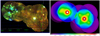 |
Fig. 3 Exposure-corrected mosaic image of the SN 1987A and SNR N132D regions (left) in three-colour presentation (red: 0.2−0.5 keV, green = 0.5−1.0 keV, blue = 1.0−2.0 keV) and a mosaic of exposure maps of all observations (right) in the entire energy range of 0.2−10.0 keV shown in linear scale in the range of 0−110 ks. |
 |
Fig. 4 Exposure-corrected mosaic image of the SN 1987A and SNR N132D regions without point sources (red: 0.2−0.5 keV, green = 0.5–1.0 keV, blue = 1.0−2.0 keV) and regions used for spectral analysis. The spectra of the regions shown in colour (30 Dor west, 30 Dor centre, 30 Dor C west, and between SNR N132D and SN 1987A in red, blue, cyan, and magenta, respectively) are shown in Fig. 6. |
3.2 Spectral analysis
Using the event files from which the point sources have been excluded, we extracted spectra in regions that were defined based on the photon statistics using the Voronoi tessellation algorithm (Cappellari & Copin 2003). For the spectral analysis, we focus on observations with SN 1987A and SNR N132D at or close to the aimpoints, which have high exposure (>20 ks, 700156, 700161, 700179). Voronoi tessellation was not performed on the entire data of each observation at once, since otherwise obviously continuous emission (e.g. in 30 Dor) was divided and merged with surrounding emission with lower brightness. Instead, we defined large regions based on similar surface brightness levels, each of which was tessellated. In general, the diffuse emission is fainter in the western region around SNR N132D. We used a signal-to-noise ratio of >50 for this region, which allows us to reach a good spatial resolution, and at the same time yields spectra with good photon statistics. The region around SN 1987A shows brighter diffuse emission, which allowed us to define smaller extraction regions with a signal-to-noise ratio of >100 (see Fig. 4).
The observational data are contaminated with particle- induced, non-X-ray background and with astrophysical X-ray background (for first studies of the background measured with eROSITA, see Freyberg et al. 2020). For the spectral analysis, all background components were modelled and fit simultaneously with the source components. The particle background dominates the data at higher energies and the higher-energy band hence allows us to determine its flux level. Therefore, to estimate the particle background we used the data up to 9.0 keV, even though no diffuse emission was observed above ~7.0 keV. The particle background consists of a continuum component that can be described with two to three power-law models with additional emission lines caused in the telescope. The astrophysical X-ray background was modelled as a combination of emission from the Local Hot Bubble, Galactic halo, and the extragalactic X-ray background. To estimate the astrophysical X-ray background, emission from non-source regions in the eROSITA EDR data from nearby observations (pointed at the globular cluster 47 Tucanae and the galaxy cluster A3158) were used. The spectral model parameters were determined by fitting the spectra of these non-source regions. For the analysis of the diffuse emission in the LMC, we fixed the model parameters for the astrophysical background and scaled it with a multiplicative constant parameter, which was free in the fit.
We analysed the spectra using XSPEC version 12.11.1. We modelled the spectrum of the diffuse emission with a combination of two thermal plasma models and a power law, absorbed by gas in the Milky Way and in the LMC. Studies of the hot ISM in the Milky Way, the Magellanic Clouds, and the nearby galaxies with Chandra, Suzaku, or XMM-Newton (e.g. Kuntz & Snowden 2010; Kavanagh et al. 2020, and references therein) have shown that the diffuse X-ray emission in the ISM of normal galaxies requires at least two thermal plasma components with different temperature: kT1 ≈ 0.2 keV consistently in most cases, most likely emission from the hot ISM in equilibrium and from unresolved stellar sources, and kT2 > 0.5 keV from regions, which experienced recent heating (i.e. H II regions, superbubbles, and SNRs) or also include unresolved binaries. For the plasma emission we tried both the collisional ionisation equilibrium model vapec2 and non-equilibrium ionisation model vnei (Borkowski et al. 2001, and references therein). Since the lower- temperature component has an ionisation timescale τ = net of ~1013 s cm−3, and is thus consistent with collisional ionisation equilibrium, while that of the higher-temperature component is not well constrained, we decided to use the results obtained with two vapec model components for further discussion. In addition, some SNRs and a few superbubbles are also known to emit significant non-thermal X-ray emission, with 30 Doradus C (30 Dor C) located close to SN 1987A being one of the only two non-thermal superbubbles known so far in the Local Group of galaxies. We therefore included a power-law component to model the emission in regions like 30 Dor C and to verify if non-thermal emission can also be detected outside the known non-thermal sources. For the foreground absorption, we included two components, one for the absorbing column in the Milky Way NH,Gal, which is fixed to the value from the newly calculated map of the Galactic NH,cold,Gal (see Sect. 2.2), and another component for the LMC with 0.5 × solar abundances. For the NH, we use the model tbvarabs (Wilms et al. 2000).
For the fits we first set all element abundances to the average value of 0.5× the solar values (Russell & Dopita 1992). We assumed the element abundances reported by Anders & Grevesse (1989). In the next step we freed the abundances of O, Ne, and Mg in the hot thermal plasma emission component one by one since there is significant emission from thermal plasma up to 2.0 keV. We verified whether the fit improves with the new free parameter using the F-test statistics. If the change was not significant, the parameter was set back to 0.5 x solar. Figure 5 shows the distribution of the values for X2/d.o.f.
In Fig. 6 we show four example spectra with the best-fit models. The upper left spectrum is taken in the western wing of the giant H II region 30 Dor, while the upper right panel shows the spectrum of the central region of 30 Dor. The lower left spectrum was extracted in the western part of the non-thermal shell of 30 Dor C, the superbubble located south-west of 30 Dor. In addition, we also show one of the spectra taken in a less active region between SN 1987A and SNR N132D, where no bright Ha structures are observed. The best-fit parameters for the spectra are listed in Table 2.
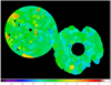 |
Fig. 5 Parameter map showing the values for X2/d.o.f. of the best-fit model for the spectra of each region. |
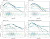 |
Fig. 6 Spectra of four regions: in the western shell inside 30 Dor (upper left), close to the centre of 30 Dor (upper right), in the western part of the non-thermal shell of 30 Dor C (lower left), and a region between SN 1987A and SNR N132D with no bright structure in Hα emission (lower right). Spectra of all TMs are shown in different colours. The thin dashed lines indicate the spectral components of the astrophysical background spectrum. The straight line shows the particle background. The source components are highlighted with thick lines (dotted: lower-temperature vapec1; dashed: higher-temperature vapec2; dash-dotted: powerlaw). |
Fit parameters.
4 Massive stars in 30 Doradus
The 30 Doradus region is known to host a large number of very massive stars (Feast et al. 1960), including the compact cluster of young massive stars RMC 136 in the centre. It contains the Wolf-Rayet star R136a1, which is one of the most massive stars detected to date (Crowther et al. 2010). Compact clusters of young massive stars are expected to be very efficient cosmic ray accelerators (for a review see Bykov 2014; Bykov et al. 2020). In X-rays bright diffuse emission has been detected from the central region in addition to point sources, which were resolved with Chandra (Townsley et al. 2006a,b).
With eROSITA, two bright sources are detected in the central region, one at the position of the star cluster RMC 136 and another source at the position of the Wolf-Rayet stars RMC 139 and RMC 140. We extracted the spectra of these two extended sources. The emission in both regions are well reproduced with thermal emission from a non-equilibrium ionisation plasma (vnei) and non-thermal emission (powerlaw). The temperature of the plasma is kT > 1 keV, and thus higher than in the surrounding regions with diffuse X-ray emission. The photon index of the power-law component is low (Γ = 1.3), indicating a hard X-ray spectrum (Table 3). Using the eROSITA spectrum we obtain a significantly enhanced abundance for Mg in both regions and for Si for RMC 136. Other elements are not well constrained due to poor photon statistics for the emission lines.
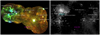 |
Fig. 7 eROSITA mosaic images in three colours (same as in Fig. 3, left) and ASKAP 888 MHz image (Pennock et al. 2021). Known SNRs are shown in white, while the SNR candidates J0529–7004 and J0538–6921 are shown in magenta and cyan, respectively. |
Fit parameters for the emission at RMC 136 and RMC 139/140.
5 Supernova remnants
In the part of the LMC that was observed with eROSITA in the early phase, there are several known SNRs, which can all be confirmed in the eROSITA data (Fig. 7). In addition, there are two sources that are known to be SNR candidates (one radio and one optical source). The analysis of the eROSITA emission of these objects is presented in the following.
 |
Fig. 8 Three-colour eROSITA image of SNR J0529–7004 (red: 0.20.5 keV, green = 0.5-1.0 keV, blue = 1.0–2.0 keV) with contours of [S II] emission (MCELS). |
5.1 SNR candidate J0529–7004
SNR candidate J0529−7004 is an arc-like structure seen in optical emission-line images with a high flux ratio of [S II]/Ha = 1. Therefore, Yew et al. (2021) have suggested it as an SNR candidate. An X-ray source was detected with ROSAT at its position (Haberl & Pietsch 1999). With eROSITA the position was observed in observation 700185. There is faint extended X-ray emission, as can be seen in the three-colour image in Fig. 8. We extracted spectra at the position of the optical SNR candidate. The local background was taken from a nearby region with no significantly enhanced emission, and was subtracted from the source spectrum. The eROSITA spectra are shown in Fig. 9 (upper panel). First, we fit the spectra with one thermal plasma model vapec or vnei, which did not yield a good fit. We therefore fit the spectrum again with a two-vapec model and obtain the best-fit with x2 = 132 and 61 degrees of freedom (d.o.f.) with the following parameters: kT. = 0.20 (0.13−0.27) keV, kT2 = 0.68 (0.62−0.74) keV. The foreground column density tends to zero with an upper limit of NH = 1.6 x 1020 cm−2. The best-fit model yields a flux (absorbed) of FX(0.2−10.0 keV) = (1.4 ± 1.0) x 10−13 erg s−1 cm−2. Due to poor photon statistics, element abundances could not be determined and were all set to 0.5 times solar. The X-ray emission and the optical [S II]/Ha flux ratio confirm this source to be an SNR.
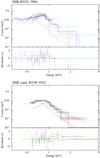 |
Fig. 9 eROSITA spectra of SNR J0529−7004 (upper panel, ObsID 700185) and SNR candidate J0538−6921 (lowerpanel, ObsID 700 161) with the best-fit two-vapec models. |
5.2 SNR candidate J0538−6921
SNR candidate J0538−6921 was detected in radio and classified as an SNR candidate (Bozzetto et al. 2017, and references therein) with a radio spectral index of α = −0.59 ± 0.04. Very faint filaments can be seen in the optical, but a clear structure indicative of an SNR is missing. In the eROSITA data (ObsID 700161), there is diffuse X-ray emission at the position of the radio candidate, but without a clear structure that could be identified as an SNR. We extracted the spectra at the position of the radio source and in a nearby background region (Fig. 9, lower panel). However, since there is an X-ray bright foreground star located in the south close to the object, it was not possible to extract the X-ray spectrum at the entire position of the radio source. The background spectrum was subtracted from the source spectrum. The best-fit parameter values for a two-vapec model with X2 = 92 and 77 d.o.f. are kT1 = 0.30 (0.27−0.33) keV, kT2 = 0.95 (0.89–1.1) keV. In this case the foreground column density is also not well constrained. The X-ray emission is very faint with a flux (absorbed) of FX(0.2–10.0 keV) = (6 ± 2) x 10−14 erg s−1 cm−2. Due to the lack of a clear structure in X-rays and the very faint flux, this object cannot be confirmed as an SNR. Since this source is located in a region with enhanced diffuse emission both in the images of the optical line emission (see Fig. 10, lower right) and those in X-rays, it is difficult to identify a possible SNR. In addition, the diffuse emission in the optical and X-rays suggest that the region is filled with ionised gas and was most likely heated by interstellar shocks in the past. In such a region the SNR would be expanding in a medium with a density that is lower than in an unshocked medium, which would explain the lack of obvious X-ray and optical emission from the SNR.
6 Discussion
We created maps for all fit parameters by filling the extraction regions with the parameter values of the best-fit models. The parameter maps for the normalisation per arcmin2 for the three source emission components are shown in Fig. 10. Normalisation in XSPEC for the thermal model vapec is defined as
![Mathematical equation: ${\rm{nor}}{{\rm{m}}_{{\rm{vapec}}}} = {1 \over {{{10}^{- 14}}\left({4\pi D_{{\rm{LMC}}}^2} \right)}}\int {{n_{\rm{e}}}{n_{\rm{H}}}{\rm{d}}V} \left[{{\rm{c}}{{\rm{m}}^{{\rm{- 5}}}}} \right],$](/articles/aa/full_html/2022/05/aa41054-21/aa41054-21-eq1.png) (1)
(1)
with ne and nH being the electron and hydrogen densities, respectively. For the power-law model the normalisation is normpowerlaw = number of photons keV−1 cm−2 s−1 at 1 keV. For the images in Fig. 10 the normalisation of the fit was divided by the size of the extraction region A in arcmin2.
6.1 Thermal component
In all regions there is significant emission from thermal plasma. We calculated the average temperature and its standard deviation from the parameter maps for kT1 and kT2, in which each pixel is filled with the best-fit parameter values. We thus obtain a mean temperature of kT1 = 0.22 keV with a standard deviation of σkT1 = 0.02 keV for the lower-temperature component and kT2 = 0.74 keV and σkT2 = 0.10 keV for the higher-temperature component. These temperature values are consistent with the results of the analysis of XMM-Newton observations of south-eastern parts of the LMC (regions around 30 Dor, in the X-ray spur, and west of them) by Knies et al. (2021). As can be seen in Fig. 10 (upper panels), the normalisation per area of the lower- temperature component (vapec1) is one order of magnitude higher than that of the higher-temperature component (vapec2).
From magnitude and colour measurements of stars in the LMC, the thickness of the disk was determined to be d = 3 ± 1 kpc at the position of SNR N132D by Subramanian & Subramaniam (2009) and Rubele et al. (2012). The volume V of the plasma in each of the spectral analysis regions can be written as
 (2)
(2)
where A is the area of the extraction region in arcmin2, DLMC = 50 kpc is the distance to the LMC, and d = 3 kpc is the thickness of the disk. By assuming a homogeneous depth of the volume, introducing a filling factor f for the plasma, and using the relation ne = 1.2nH, we can write
 (3)
(3)
With the mean value of normvapec1/A = (1.6 ± 1.0) ×10−5 cm−5 arcmin−2 (fit uncertainty of ~10−4 and standard deviation of 0.4 × 10⁻⁵) for the brighter, lower-temperature vapec1 component in the western regions around SNR N132D, we get a mean density of nH,1 = (3.1 ± 1.5) × 10−4f−1/2 cm−2. We assume that the emitting plasma can be regarded as an ideal gas with the pressure
 (4)
(4)
where kB is the Boltzman constant. The temperature T1 of vapec1 and the hydrogen number density nH,1 derived from the normalisation yield a mean pressure of  K in the western regions. This pressure is consistent with the thermal pressure in the disk of the Milky Way (Cox 2005).
The higher normalisations of the thermal emission models in the eastern regions around 30 Dor compared to the regions around SNR N132D imply that the emission is brighter in and around 30 Dor and in the south-east than it is towards the west. These are the regions that also show bright line emission in the optical, as can be confirmed in the images of the Magellanic Clouds Emission Line Survey (MCELS, see Fig. 10, lower right, Smith et al. 2004). In the eROSITA mosaic images (Fig. 3) the emission in these regions appears to be fainter than or as faint as in the west. At the same time, the regions also appear green in the three-colour presentation, suggesting that the observed variation in surface brightness and colour is due to higher absorption. This will be discussed further in Sect. 6.4.
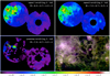 |
Fig. 10 Parameter maps of the normalisation per arcmin2, illustrating the surface brightness of the diffuse emission, for the two thermal components (vapec1, vapec2) and the powerlaw component. The images are shown in log-scale. The letters W, X, Y, Z in the labels correspond to the exponents of the marks of the colour scale. The red plus sign indicates the position of the star cluster RMC 136,the yellow cross that of SNR/PWN N157B. The lower right panel shows Hα (red), [S II] (green), and [O III] (blue) images of MCELS in three-colour presentation. |
6.2 Non-thermal component
Non-thermal emission is observed significantly in the superbubble 30 Dor C (see Fig. 10, lower left, and Fig. 6, lower left). The photon index obtained from the eROSITA data is Γ = 2.5 ± 0.5, which is in agreement with earlier studies (e.g. Kavanagh et al. 2015, 2019, and references therein). Recently, in a combined XMM-Newton and NuSTAR analysis, Lopez et al. (2020) showed that the complete shell of 30 Dor C is detected up to 20 keV. The authors found that contrary to prior studies, their region D (part of 30 Dor C West here) requires a thermal component of kT = 0.86 ± 0.01 keV, which is consistent with the eROSITA fit with the temperature of 0.62 (0.28−1.1) keV given in Table 2. The photon indices of a power-law component obtained by eROSITA for the entire 30 Dor C West region is Γ = 2.4 (2.32.6), which is somewhat higher than the value of 2.12 ± 0.02 obtained for region D, but consistent with 2.39 ± 0.03 obtained for region C, which were both covered by our 30 Dor C West region. SNR MCSNR J0536-6913, which was found earlier with XMM-Newton (Kavanagh et al. 2015; Babazaki et al. 2018) and is apparent in the eROSITA image (Fig. 7, left), was not detected above 8 keV in the NuSTAR observation.
Synchrotron radiation of very high-energy electrons and positrons is a likely source of a substantial amount of the observed non-thermal X-rays. The high-energy leptonic component is accelerated in supernova remnants, superbubbles, and pulsar wind nebulae, and can be produced by inelastic collisions of cosmic ray nuclei. The high-energy leptons producing the synchrotron X-rays simultaneously up-scatter photons from ambient radiation field. The inverse-Compton radiation from multi-TeV leptons producing the observed X-ray synchrotron apparently contribute to the TeV gamma-ray emission detected from the pulsar wind nebula (PWN) N157B and the superbubble 30 Dor C by the ground-based Cherenkov gamma-ray telescope H.E.S.S. (see e.g. H.E.S.S. Collaboration 2015). Observations with H.E.S.S. yielded a luminosity of ~0.9 x 1035 erg s−1 for 30 Dor C for the 1–10 TeV gamma-ray band with a power-law distribution of a photon index 2.6 ± 0.2, which is consistent with the photon index of X-rays detected by eROSITA in 30 Dor C west (see Table 2). The observed TeV emission apart from the inverse-Compton mechanism mentioned earlier could originate from the decay of neutral pions produced in the inelastic collisions of relativistic nuclei with the ambient matter (the so-called hadronic scenario). While the expected fluxes in the leptonic scenario can explain the observed fluxes of X-rays and TeV gamma-rays, as well as the measured widths of the non-thermal X-ray filaments (Kavanagh et al. 2019), the hadronic origin of the observed gamma-rays cannot be excluded (see e.g. H.E.S.S. Collaboration 2015).
There is also significant non-thermal emission in the central region of 30 Dor (see Fig. 6, upper right and Table 2). This non-thermal component can indicate some contamination by emission from the composite SNR with a PWN N157B, located south-west of the region (yellow cross in Fig. 10, lower left). The emission of N157B itself was removed when point and point-like sources were cut out from the event files. The X-ray spectrum of N157B consists of thermal emission of the SNR and the dominant non-thermal power-law emission from the pulsar and the PWN with a photon index of Γ = 2.29 (+0.05, −0.06), while the pulsar shows a power-law emission with Γ = 1.73 (+0.11, −0.06) (Chen et al. 2006). The high lower limit of Γ > 2.5 for the photon index for the non-thermal emission detected inside 30 Dor suggests that it is not caused by emission from N157B. It should be noted, however, that the gamma-ray spectrum of N157B detected by H.E.S.S. (H.E.S.S. Collaboration 2012) can be described well by a power-law component with a photon index Γ = 2.8 ± 0.2stat ± 0.3syst in the energy range between 600 GeV and 12 TeV.
Since non-thermal emission is also found to the north of the super-star cluster RMC 136 (red plus sign) and possibly in a larger region towards the east, it might also be caused by particles that were accelerated in the shocks of the winds of massive stars inside RMC 136 and are diffusing inside and probably also outside of the nebula. Diffuse non-thermal X-ray emission was detected with Chandra from the most massive Galactic star cluster Westerlund 1 (Muno et al. 2006). They estimated the X-ray luminosity to be about 3 x 1034 erg s−1, and found that while the photon index of the power-law X-ray component is Γ = 2.7 ± 0.2 within the circle of 1′ radius around the cluster, the spectrum gets harder with  in the annulus between 1′ and 2′ and even
  between 2′ and 3.5′. Possible mechanisms of the origin of the non-thermal emission in the clusters of young massive stars were discussed by Bykov (2014). Further studies will be performed in the future when additional data of the eROSITA All-Sky Survey is available.
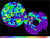 |
Fig. 11 Parameter map of fitted Ne abundances (normalised to solar abundance). The white boxes are the regions used for the calculation of the star formation rate (Fig. 12). |
6.3 Element abundances
The eROSITA spectra suggest that the element abundance of neon is enhanced in the regions around 30 Dor (Table 2, Fig. 11). The mean value of the Ne abundance around 30 Dor is 2.25 times solar, with a mean value of the 90% error of 1.16. In the regions around N132D the mean Ne abundance is 1.93 and the mean value of the 90% error is 0.70. In total, a free parameter for the Ne abundance improved the fit in 235 regions, while for 151 regions, the fit was consistent with a Ne abundance of 0.5 times solar.
There are also line transitions of oxygen and magnesium in the energy range of 0.4−2.0 keV, in which eROSITA has the highest response. However, the O and Mg lines are contaminated by background emission (solar-wind charge exchange lines and Al Kα line at 1.486 keV from the detector, respectively), which were included in the background model as free components. Therefore, the O and Mg abundances are not well constrained. The O abundance was fixed to 0.5 times solar in all regions since freeing the parameter did not improve the fit. In the case of Mg, in the east, the mean value is 1.62 with a mean 90% error of 0.76 (the Mg abundance was free in 70 out of 247 regions), and in the west the mean abundance is 1.59 with a mean 90% error of 0.35 (free in only 4 out of 139 regions). Therefore, O is consistent with 0.5 times the solar value in all regions, and there is no clear gradient seen in the Mg abundance.
To understand the possible origin of Ne, we calculated and plotted the star formation rate in these two areas in LMC (marked with boxes in Fig. 11) based on the star formation rates of Harris & Zaritsky (2009) (Fig. 12). In the eastern region (labelled ‘1’), star formation has been ongoing over the last 106−107 yr, producing a large number of young massive stars that have created the large and complex H II regions. Most likely, the ISM has also been enriched by stellar winds and supernovae of these massive stars.
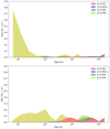 |
Fig. 12 Star formation rate from Harris & Zaritsky (2009) in the regions in Fig. 11 (upper: 1, lower: 2). |
6.4 Foreground absorption in the LMC
The fits show that the foreground column density NH,LMC in the LMC is higher around 30 Dor (see Fig. 13) than in the west, also indicated by the green colour of the X-ray image. The values obtained from the analysis of the X-ray spectrum taken with eROSITA is in very good agreement with the NH,cold,LMC in the LMC obtained from the distribution of cold matter (Sect. 2.2), as can be seen in Fig. 13. This agreement between the values derived from the X-ray analysis and measured directly from the cold medium seen over a large area of >1° is remarkable, and shows the advantage of the large FOV and the high sensitivity of eROSITA in the energy band of 0.2-2.0 keV.
Together with the high normalisation (and thus intrinsic flux) of the emission in the same regions, the enhanced NH,LMC indicates that the hot X-ray emitting plasma is located behind a high-density region. The same stars that created the giant H II region 30 Dor and the other H II structures in its surroundings are the likely sources of the hot interstellar plasma. This result corroborates nicely the scenario of the collision of large H I structures in the LMC for the origin of 30 Dor and the star-forming regions south of 30 Dor presented by Fukui et al. (2017) and recently confirmed by Knies et al. (2021) based on a multi-wavelength study of the south-eastern part of the LMC, in particular the X-ray spur. A large H I component, called the L-component encountered the H I component in the disk of the LMC (D-component) in the past, starting roughly at the position where 30 Dor is observed now. The collision continued south of 30 Dor where young massive stars and, even further to the south, a long ridge of dust and CO clouds along with star-forming regions are found next to the X-ray spur. The L- component is now located in front of the disk of the LMC at the position of 30 Dor, which corresponds to the eastern part of the eROSITA observations that we analysed, and absorbs the emission from 30 Dor and from the sources and the hot interstellar plasma around it.
7 Summary
The first-light observation of eROSITA was pointed at SN 1987A and has provided us with an impressive X-ray view of a large number of sources and complex diffuse emission in the LMC in a large 1° diameter field. This field includes several prominent objects: the giant H II-region 30 Dor, the non-thermal superbubble 30 Dor C, and bright SNRs and pulsars. At a distance of about 1.5° from SN 1987A there is SNR N132D, which is the brightest X-ray SNR in the LMC. As one of the X-ray calibration sources, SNR N132D and its surroundings have also been observed in the early phase of the eROSITA mission multiple times. In this paper we have presented the study of the diffuse X-ray emission in the LMC detected in these early eROSITA observations.
To understand the properties of the hot interstellar plasma and the processes that form it, we have been studying SNRs and superbubbles in the Magellanic Clouds using XMM-Newton and Chandra (e.g. Sasaki et al. 2011; Kavanagh et al. 2012, 2015, 2019; Warth et al. 2014). Due to the much smaller FOV of these X-ray observatories, our studies have so far had to focus on a small number of selected objects. The large FOV of eROSITA and the high sensitivity at energies below 2 keV combined with the much better spatial and spectral resolution than ROSAT, which was the last X-ray observatory that performed a survey of the entire LMC (for a study of the diffuse emission, see Sasaki et al. 2002), makes eROSITA the perfect instrument with which to study the hot ISM in our neighbour galaxy. Thanks to the early commissioning and calibration observations, we obtained a set of long exposures with eROSITA towards the most interesting regions of the LMC.
We have analysed the data of 11 eROSITA observations by eliminating all point and point-like sources and focusing on the diffuse emission. Using a tessellation algorithm, we divided the data into small regions with a signal-to-noise ratio of >100 and >50 around SN 1987A and SNR N132D, respectively. The spectra of the diffuse emission in these regions were analysed assuming a combination of a two-component thermal plasma and one non-thermal emission model. Maps of the parameter values obtained for the best-fit model have been created and studied. The results of the spectral analysis are as follows:
We detect emission from thermal plasma in the ISM in the LMC in all regions. There is dominant emission from a low-temperature component with kT = 0.2 keV and another lower-brightness thermal component with kT ≈ 0.7 keV. The interstellar density and pressure derived from the parameters of the major lower-temperature component are consistent with values measured in the Milky Way.
The emission from the higher-temperature thermal component is stronger in the environment of 30 Dor, suggesting that the young stellar population has caused recent heating.
In these regions, the element abundances also seem to be enhanced, as indicated by the high Ne abundance. Most likely, the ISM has been enriched by the stellar winds and supernovae of massive stars.
In addition, significant non-thermal emission is confirmed in the superbubble 30 Dor C. There are indications of the presence of non-thermal emission also east of 30 Dor, which requires further investigation.
The X-ray spectral analysis yields an absorbing column density NH in the LMC, which is surprisingly consistent with the column density derived from the measurements of H I and the gas-to-dust ratio at low energies. This is the first time that the foreground column density has been determined through X-ray spectroscopy over such a large contiguous field and is in agreement with direct measurements from the cold interstellar medium.
We analysed the spectra of the massive stellar cluster RMC 136 and the emission from the Wolf-Rayet stars RMC 139 and RMC 140. The emission is nicely reproduced by a model consisting of emission from a non-ionisation equilibrium plasma with kT > 1 keV and τ = net ≈ 1011 s cm−3 and a power-law component with Γ = 1.3.
Based on eROSITA image and spectroscopy, we confirm SNR J529-7004 as a new SNR in the LMC.
As we have been anticipating during the years of preparations for the eROSITA mission, eROSITA is the perfect telescope for studying the ISM at high energies. Currently, eROSITA is carrying out a total of eight all-sky surveys over a period of four years. We will extend the study of the ISM in the LMC based on the eROSITA all-sky survey data. In addition, the eROSITA all-sky survey will also allow us to study the hot phase of the ISM in the SMC.
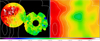 |
Fig. 13 NH,LMC in the LMC obtained from the fit of the eROSITA spectra (left) vs. NH.cold,LMC directly calculated from cold H I and dust (right) in cm–2. Both images are shown in log-scale using the same lower and upper cuts. The contours of NH,cold,LMC are plotted in both panels. |
Acknowledgements
This work is based on data from eROSITA, the soft X-ray instrument aboard SRG, a joint Russian-German science mission supported by the Russian Space Agency (Roskosmos), in the interests of the Russian Academy of Sciences represented by its Space Research Institute (IKI), and the Deutsches Zentrum fur Luft- und Raumfahrt (DLR). The SRG spacecraft was built by Lavochkin Association (NPOL) and its subcontractors, and is operated by NPOL with support from the Max Planck Institute for Extraterrestrial Physics (MPE). The development and construction of the eROSITA X-ray instrument was led by MPE, with contributions from the Dr. Karl Remeis Observatory Bamberg & ECAP (FAU Erlangen-Nurnberg), the University of Hamburg Observatory, the Leibniz Institute for Astrophysics Potsdam (AIP), and the Institute for Astronomy and Astrophysics of the University of Tubingen, with the support of DLR and the Max Planck Society. The Argelander Institute for Astronomy of the University of Bonn and the Ludwig Maximilians Universität Munich also participated in the science preparation for eROSITA. The eROSITA data shown here were processed using the eSASS/NRTA software system developed by the German eROSITA consortium. The Australian SKA Pathfinder is part of the Australia Telescope National Facility (ATNF) which is managed by CSIRO. Operation of ASKAP is funded by the Australian Government with support from the National Collaborative Research Infrastructure Strategy. ASKAP uses the resources of the Pawsey Supercomputing Centre. Establishment of ASKAP, the Murchison Radio-astronomy Observatory (MRO) and the Pawsey Supercomputing Centre are initiatives of the Australian Government, with support from the Government of Western Australia and the Science and Industry Endowment Fund. This paper includes archived data obtained through the CSIRO ASKAP Science Data Archive (CASDA). We acknowledge the Wajarri Yamatji as the traditional owners of the Observatory site. MCELS was funded through the support of the Dean B. McLaughlin fund at the University of Michigan and through NSF grant 9540747. M.S. acknowledges support by the Deutsche Forschungsgemeinschaft through the Heisenberg professor grant SA 2131/12-1. A.M.B. was supported by the RSF grant 21-72-20020.
References
- Anders, E., & Grevesse, N. 1989, Geochim. Cosmochim. Acta, 53, 197 [Google Scholar]
- Babazaki, Y., Mitsuishi, I., Matsumoto, H., et al. 2018, ApJ, 864, 12 [NASA ADS] [CrossRef] [Google Scholar]
- Blondiau, M. J., Kerp, J., Mebold, U., & Klein, U. 1997, A&A, 323, 585 [NASA ADS] [Google Scholar]
- Borissova, J., Minniti, D., Rejkuba, M., et al. 2004, A&A, 423, 97 [NASA ADS] [CrossRef] [EDP Sciences] [Google Scholar]
- Borissova, J., Minniti, D., Rejkuba, M., & Alves, D. 2006, A&A, 460, 459 [NASA ADS] [CrossRef] [EDP Sciences] [Google Scholar]
- Borkowski, K. J., Lyerly, W. J., & Reynolds, S. P. 2001, ApJ, 548, 820 [Google Scholar]
- Bozzetto, L. M., Filipović, M. D., Vukotić, B., et al. 2017, ApJS, 230, 2 [NASA ADS] [CrossRef] [Google Scholar]
- Brunner, H., Liu, T., Lamer, G., et al. 2022, A&A, 661, A1 (eROSITA EDR SI) [NASA ADS] [CrossRef] [EDP Sciences] [Google Scholar]
- Brüns, C., Kerp, J., Staveley-Smith, L., et al. 2005, A&A, 432, 45 [CrossRef] [EDP Sciences] [Google Scholar]
- Bykov, A. M. 2014, A&ARv, 22, 77 [NASA ADS] [CrossRef] [Google Scholar]
- Bykov, A. M., Marcowith, A., Amato, E., et al. 2020, Space Sci. Rev., 216, 42 [CrossRef] [Google Scholar]
- Cappellari, M., & Copin, Y. 2003, MNRAS, 342, 345 [Google Scholar]
- Cardelli, J. A., Clayton, G. C., & Mathis, J. S. 1989, ApJ, 345, 245 [Google Scholar]
- Chen, Y., Wang, Q. D., Gotthelf, E. V., et al. 2006, ApJ, 651, 237 [NASA ADS] [CrossRef] [Google Scholar]
- Cox, D. P. 2005, ARA&A, 43, 337 [Google Scholar]
- Crowther, P. A., Schnurr, O., Hirschi, R., et al. 2010, MNRAS, 408, 731 [Google Scholar]
- de Grijs, R., Wicker, J. E., & Bono, G. 2014, AJ, 147, 122 [Google Scholar]
- de Vaucouleurs, G. 1955, AJ, 60, 126 [NASA ADS] [CrossRef] [Google Scholar]
- Feast, M. W., Thackeray, A. D., & Wesselink, A. J. 1960, MNRAS, 121, 337 [NASA ADS] [CrossRef] [Google Scholar]
- Freyberg, M., Perinati, E., Pacaud, F., et al. 2020, SPIE Conf. Ser., 11444, 114441 [NASA ADS] [Google Scholar]
- Fujimoto, M., & Noguchi, M. 1990, PASJ, 42, 505 [Google Scholar]
- Fukui, Y., Mizuno, N., Yamaguchi, R., et al. 1999, PASJ, 51, 745 [Google Scholar]
- Fukui, Y., Kawamura, A., Minamidani, T., et al. 2008, ApJS, 178, 56 [Google Scholar]
- Fukui, Y., Tsuge, K., Sano, H., et al. 2017, PASJ, 69, L5 [Google Scholar]
- Güver, T., & Özel, F. 2009, MNRAS, 400, 2050 [Google Scholar]
- H.E.S.S. Collaboration (Abramowski, A., et al.) 2012, A&A, 545, L2 [NASA ADS] [CrossRef] [EDP Sciences] [Google Scholar]
- H.E.S.S. Collaboration (Abramowski, A., et al.) 2015, Science, 347, 406 [NASA ADS] [CrossRef] [Google Scholar]
- Haberl, F., & Pietsch, W. 1999, A&AS, 139, 277 [NASA ADS] [CrossRef] [EDP Sciences] [Google Scholar]
- Haberl, F., Maitra, C., Carpano, S., et al. 2022, A&A, 661, A25 (eROSITA EDR SI) [NASA ADS] [CrossRef] [EDP Sciences] [Google Scholar]
- Harris, J., & Zaritsky, D. 2009, AJ, 138, 1243 [NASA ADS] [CrossRef] [Google Scholar]
- HI4PI Collaboration (Ben Bekhti, N., et al.) 2016, A&A, 594, A116 [NASA ADS] [CrossRef] [EDP Sciences] [Google Scholar]
- Hotan, A. W., Bunton, J. D., Chippendale, A. P., et al. 2021, PASA, 38, e009 [NASA ADS] [CrossRef] [Google Scholar]
- Johnston, S., Taylor, R., Bailes, M., et al. 2008, Exp. Astron., 22, 151 [Google Scholar]
- Joshi, Y. C., & Panchal, A. 2019, A&A, 628, A51 [NASA ADS] [CrossRef] [EDP Sciences] [Google Scholar]
- Kalberla, P. M. W., & Haud, U. 2015, A&A, 578, A78 [NASA ADS] [CrossRef] [EDP Sciences] [Google Scholar]
- Kalberla, P. M. W., & Kerp, J. 2009, ARA&A, 47, 27 [NASA ADS] [CrossRef] [Google Scholar]
- Kavanagh, P. J., Sasaki, M., & Points, S. D. 2012, A&A, 547, A19 [NASA ADS] [CrossRef] [EDP Sciences] [Google Scholar]
- Kavanagh, P. J., Sasaki, M., Bozzetto, L. M., et al. 2015, A&A, 573, A73 [NASA ADS] [CrossRef] [EDP Sciences] [Google Scholar]
- Kavanagh, P. J., Vink, J., Sasaki, M., et al. 2019, A&A, 621, A138 [NASA ADS] [CrossRef] [EDP Sciences] [Google Scholar]
- Kavanagh, P. J., Sasaki, M., Breitschwerdt, D., et al. 2020, A&A, 637, A12 [EDP Sciences] [Google Scholar]
- Kim, S., Staveley-Smith, L., Dopita, M. A., et al. 2003, ApJS, 148, 473 [Google Scholar]
- Knies, J. R., Sasaki, M., Fukui, Y., et al. 2021, A&A, 648, A90 [NASA ADS] [CrossRef] [EDP Sciences] [Google Scholar]
- Kuntz, K. D., & Snowden, S. L. 2010, ApJS, 188, 46 [NASA ADS] [CrossRef] [Google Scholar]
- Lopez, L. A., Grefenstette, B. W., Auchettl, K., Madsen, K. K., & Castro, D. 2020, ApJ, 893, 144 [NASA ADS] [CrossRef] [Google Scholar]
- Luks, T., & Rohlfs, K. 1992, A&A, 263, 41 [NASA ADS] [Google Scholar]
- Maitra, C., Haberl, F., Sasaki, M., et al. 2022, A&A, 661, A30 (eROSITA EDR SI) [NASA ADS] [CrossRef] [EDP Sciences] [Google Scholar]
- Mathewson, D. S., Cleary, M. N., & Murray, J. D. 1974, ApJ, 190, 291 [NASA ADS] [CrossRef] [Google Scholar]
- Merloni, A., Predehl, P., Becker, W., et al. 2012, ArXiv e-prints [arXiv:1209.3114] [Google Scholar]
- Mizuno, N., Yamaguchi, R., Mizuno, A., et al. 2001, PASJ, 53, 971 [NASA ADS] [Google Scholar]
- Muno, M. P., Law, C., Clark, J. S., et al. 2006, ApJ, 650, 203 [NASA ADS] [CrossRef] [Google Scholar]
- Pennock, C. M., van Loon, J.T., Filipović, M. D., et al. 2021, MNRAS, 506, 3540 [NASA ADS] [CrossRef] [Google Scholar]
- Points, S. D., Chu, Y. H., Snowden, S. L., & Smith, R. C. 2001, ApJS, 136, 99 [NASA ADS] [CrossRef] [Google Scholar]
- Predehl, P., Andritschke, R., Arefiev, V., et al. 2021, A&A, 647, A1 [EDP Sciences] [Google Scholar]
- Rubele, S., Kerber, L., Girardi, L., et al. 2012, A&A, 537, A106 [NASA ADS] [CrossRef] [EDP Sciences] [Google Scholar]
- Russell, S. C., & Dopita, M. A. 1992, ApJ, 384, 508 [NASA ADS] [CrossRef] [Google Scholar]
- Sasaki, M., Haberl, F., & Pietsch, W. 2002, A&A, 392, 103 [NASA ADS] [CrossRef] [EDP Sciences] [Google Scholar]
- Sasaki, M., Breitschwerdt, D., Baumgartner, V., & Haberl, F. 2011, A&A, 528, A136 [NASA ADS] [CrossRef] [EDP Sciences] [Google Scholar]
- Schlafly, E. F., & Finkbeiner, D. P. 2011, ApJ, 737, 103 [Google Scholar]
- Schlegel, D. J., Finkbeiner, D. P., & Davis, M. 1998, ApJ, 500, 525 [Google Scholar]
- Smith, R. C., Points, S., Aguilera, C., et al. 2004, AAS Meet. Abs., 205, 101.08 [NASA ADS] [Google Scholar]
- Subramanian, S., & Subramaniam, A. 2009, A&A, 496, 399 [NASA ADS] [CrossRef] [EDP Sciences] [Google Scholar]
- Townsley, L. K., Broos, P. S., Feigelson, E. D., et al. 2006a, AJ, 131, 2140 [Google Scholar]
- Townsley, L. K., Broos, P. S., Feigelson, E. D., Garmire, G. P., & Getman, K. V. 2006b, AJ, 131, 2164 [NASA ADS] [CrossRef] [Google Scholar]
- Warth, G., Sasaki, M., Kavanagh, P. J., et al. 2014, A&A, 567, A136 [NASA ADS] [CrossRef] [EDP Sciences] [Google Scholar]
- Weingartner, J. C., & Draine, B. T. 2001, ApJ, 548, 296 [Google Scholar]
- Wilms, J., Allen, A., & McCray, R. 2000, ApJ, 542, 914 [Google Scholar]
- Winkel, B., Kerp, J., Flöer, L., et al. 2016, A&A, 585, A41 [NASA ADS] [CrossRef] [EDP Sciences] [Google Scholar]
- Yew, M., Filipović, M. D., Stupar, M., et al. 2021, MNRAS, 500, 2336 [Google Scholar]
- Youssoufi, D. E., Cioni, M.-R.L., Bell, C. P. M., et al. 2019, IAU Symp. 344, 66 [NASA ADS] [Google Scholar]
All Tables
All Figures
|
Fig. 1 H I velocity profile at an example position in the LMC (RA = 85.75°, Dec = -70.20°) |
| In the text | |
|
Fig. 2 Spatial distribution the Milky Way’s NHI column density for VLSR = −155 to +80 kms−1 above a threshold of NHI = 3 x 1019 cm−2 with a maximum of 1 x 1021 cm−2. Superimposed as contours is the spatial distribution of the Milky Way gas with excess optical extinction derived from the NHI/AV ratio (see text for details). The contours correspond to NH2 = 5 × 1019 cm−2 and to 1, 2, and 3 x 1020 cm−2. The LMC is located at l = 280°, b = -33°; the SMC at l = 302°, b = −44°. The yellow ellipse indicates the area observed with eROSITA. |
| In the text | |
|
Fig. 3 Exposure-corrected mosaic image of the SN 1987A and SNR N132D regions (left) in three-colour presentation (red: 0.2−0.5 keV, green = 0.5−1.0 keV, blue = 1.0−2.0 keV) and a mosaic of exposure maps of all observations (right) in the entire energy range of 0.2−10.0 keV shown in linear scale in the range of 0−110 ks. |
| In the text | |
|
Fig. 4 Exposure-corrected mosaic image of the SN 1987A and SNR N132D regions without point sources (red: 0.2−0.5 keV, green = 0.5–1.0 keV, blue = 1.0−2.0 keV) and regions used for spectral analysis. The spectra of the regions shown in colour (30 Dor west, 30 Dor centre, 30 Dor C west, and between SNR N132D and SN 1987A in red, blue, cyan, and magenta, respectively) are shown in Fig. 6. |
| In the text | |
|
Fig. 5 Parameter map showing the values for X2/d.o.f. of the best-fit model for the spectra of each region. |
| In the text | |
|
Fig. 6 Spectra of four regions: in the western shell inside 30 Dor (upper left), close to the centre of 30 Dor (upper right), in the western part of the non-thermal shell of 30 Dor C (lower left), and a region between SN 1987A and SNR N132D with no bright structure in Hα emission (lower right). Spectra of all TMs are shown in different colours. The thin dashed lines indicate the spectral components of the astrophysical background spectrum. The straight line shows the particle background. The source components are highlighted with thick lines (dotted: lower-temperature vapec1; dashed: higher-temperature vapec2; dash-dotted: powerlaw). |
| In the text | |
|
Fig. 7 eROSITA mosaic images in three colours (same as in Fig. 3, left) and ASKAP 888 MHz image (Pennock et al. 2021). Known SNRs are shown in white, while the SNR candidates J0529–7004 and J0538–6921 are shown in magenta and cyan, respectively. |
| In the text | |
|
Fig. 8 Three-colour eROSITA image of SNR J0529–7004 (red: 0.20.5 keV, green = 0.5-1.0 keV, blue = 1.0–2.0 keV) with contours of [S II] emission (MCELS). |
| In the text | |
|
Fig. 9 eROSITA spectra of SNR J0529−7004 (upper panel, ObsID 700185) and SNR candidate J0538−6921 (lowerpanel, ObsID 700 161) with the best-fit two-vapec models. |
| In the text | |
|
Fig. 10 Parameter maps of the normalisation per arcmin2, illustrating the surface brightness of the diffuse emission, for the two thermal components (vapec1, vapec2) and the powerlaw component. The images are shown in log-scale. The letters W, X, Y, Z in the labels correspond to the exponents of the marks of the colour scale. The red plus sign indicates the position of the star cluster RMC 136,the yellow cross that of SNR/PWN N157B. The lower right panel shows Hα (red), [S II] (green), and [O III] (blue) images of MCELS in three-colour presentation. |
| In the text | |
|
Fig. 11 Parameter map of fitted Ne abundances (normalised to solar abundance). The white boxes are the regions used for the calculation of the star formation rate (Fig. 12). |
| In the text | |
|
Fig. 12 Star formation rate from Harris & Zaritsky (2009) in the regions in Fig. 11 (upper: 1, lower: 2). |
| In the text | |
|
Fig. 13 NH,LMC in the LMC obtained from the fit of the eROSITA spectra (left) vs. NH.cold,LMC directly calculated from cold H I and dust (right) in cm–2. Both images are shown in log-scale using the same lower and upper cuts. The contours of NH,cold,LMC are plotted in both panels. |
| In the text | |
Current usage metrics show cumulative count of Article Views (full-text article views including HTML views, PDF and ePub downloads, according to the available data) and Abstracts Views on Vision4Press platform.
Data correspond to usage on the plateform after 2015. The current usage metrics is available 48-96 hours after online publication and is updated daily on week days.
Initial download of the metrics may take a while.