| Issue |
A&A
Volume 661, May 2022
|
|
|---|---|---|
| Article Number | A151 | |
| Number of page(s) | 24 | |
| Section | Galactic structure, stellar clusters and populations | |
| DOI | https://doi.org/10.1051/0004-6361/201936393 | |
| Published online | 24 May 2022 | |
Gaia-predicted brown dwarf detection rates around FGK stars in astrometry, radial velocity, and photometric transits
1
Department of Astronomy, University of Geneva, Ch. Pegasi 51, 1290 Versoix, Switzerland
e-mail: This email address is being protected from spambots. You need JavaScript enabled to view it.
2
Department of Astronomy, University of Geneva, Ch. d’Ecogia 16, 1290 Versoix, Switzerland
3
School of Physics, University College Dublin, Ireland
4
Lund Observatory, Department of Astronomy and Theoretical Physics, Lund University, Box 43 22100 Lund, Sweden
Received:
28
July
2019
Accepted:
26
September
2021
Abstract
Context. After more than two decades of relevant radial velocity surveys, the current sample of known brown dwarfs (BDs) around FGK stars is only of the order of 100, limiting our understanding of their occurrence rate, properties, and formation. The ongoing ESA mission Gaia has already collected more than its nominal 5 years of mission data, and is expected to operate for up to 10 years in total. Its exquisite astrometric precision allows for the detection of (unseen) companions down to the Jupiter-mass level, allowing the efficient detection of large numbers of BDs. Additionally, its low-accuracy multi-epoch radial velocity measurements for GRVS < 12 can provide additional detections or constraints for the more massive BDs, while a further small sample will have detectable transits in Gaia photometry.
Aims. Using detailed simulations, we provide an assessment of the number of BDs that could be discovered using Gaia astrometry, radial velocity, and photometric transits around main sequence (V) and subgiant (IV) FGK host stars for the nominal five-year and extended ten-year mission.
Methods. Using a robust Δχ2 statistic we analyse the BD companion detectability from the Besançon Galaxy population synthesis model for G = 10.5 − 17.5 mag, complemented by Gaia DR2 data for G < 10.5, using the latest Gaia performance and scanning law, and literature-based BD-parameter distributions.
Results. We report here only reliable detection numbers with Δχ2 > 50 for a five-year mission, and those in square brackets are for a ten-year mission. For astrometry alone, we expect 28 000–42 000 [45 000–55 000] detections out to several hundred parsecs [up to more than a kiloparsec]. The majority of these have G ∼ 14 − 15 [14 − 16] and periods of greater than 200 d, extending up to the longest simulated periods of 5 yr. Gaia radial velocity time-series for GRVS < 12 (G ≲ 12.7), should allow the detection of 830–1100 [1500–1900] BDs, most having orbital periods of < 10 days, and being amongst the most massive BDs (55 − 80MJ), though several tens will extend down to the ‘desert’ and lowest BD masses. Systems with at least three photometric transits with S/N > 3 are expected for 720–1100 [1400–2300] BDs, averaging at 4–5 [5–6] transits per source. The combination of astrometric and radial velocity detections should yield some 370–410 [870–950] detections. Perhaps 17–27 [35–56] BDs will have both transit and radial velocity detections, while both transits and astrometric detection will lead to a meagre 1–3 [4–6] detection(s).
Conclusions. Though the above numbers are affected by ±50% uncertainty due to the uncertain occurrence rate and period distribution of BDs around FGK host stars, detections of BDs with Gaia will number in the tens of thousands, enlarging the current BD sample by at least two orders of magnitude, allowing us to investigate the BD fraction and orbital architectures as a function of host stellar parameters in greater detail than every before.
Key words: astrometry / planets and satellites: general / space vehicles: instruments
© ESO 2022
1. Introduction
Brown dwarf (BD) companions with orbital periods of ≲10 yr are within the range of sensitivity and time-span of various long-running radial velocity surveys (e.g. Hatzes 2016; Díaz 2018; Figueira 2018; Oshagh 2018). But despite the many thousands of stars surveyed to date, less than 100 BD companions around solar-type stars are currently known (e.g. Ma & Ge 2014; Grieves et al. 2017). This reinforces the evidence for a BD ‘desert’, that is, the general absence of companions in the mass range 10 − 80MJ, being most pronounced between 30 and 55MJ (Marcy & Butler 2000; Grether & Lineweaver 2006).
The low-mass BD distribution seems to be the high-mass tail of the planetary distribution function (e.g. Sahlmann et al. 2011), while the high-mass BD distribution seems to be the low-mass tail of the stellar binary distribution function (Duquennoy & Mayor 1991; Tokovinin 1992; Perryman 2018, Sect. 2.7.1). This suggests that formation scenarios that populate the adopted BD mass range have diminishing efficiency toward the BD desert (Grether & Lineweaver 2006; Sozzetti & Desidera 2010; Sahlmann et al. 2011; Ma & Ge 2014; Chabrier et al. 2014; Bouchy et al. 2016; Santerne et al. 2016; Troup et al. 2016; Wilson et al. 2016; Borgniet et al. 2017; Grieves et al. 2017). Sahlmann et al. (2011) provide an upper limit on the occurrence rate of tight-orbit (P ≲ 300 d) BD companions around solar-type stars of 0.3%–0.6%, illustrating that to significantly increase the statistics of BDs, one needs to survey millions of host stars.
So far, the ongoing Gaia ESA mission (Gaia Collaboration 2016a) has provided the scientific community with three data releases (Gaia Collaboration 2016b, 2018, 2021) containing information on over a billion sources on the sky based on data spanning 13, 22, and 33 months of observation, respectively. For all sources, Gaia measures the astrometric position, three-band (spectro)photometry, and radial velocities (for GRVS ≤ 16 mag Sartoretti et al. 2018)1 (almost) simultaneously. For the nominal five-year mission, this averages to about about 70 epochs, increasing linearly with time during its extended mission.
These three measurements in principle provide three distinct discovery methods for any orbiting companions to main sequence stars, with the astrometric and radial velocity measurements probing the dynamical reflex motion of the host star, and the photometric measurements yielding transit information. Here, we consider detection yields from these approaches separately, and also in combination.
Estimation of the orbital parameters of astrometric BDs using Gaia is roughly limited to companions with shorter orbital periods than the mission length, and therefore a possible extension providing up to ten years of Gaia data would be greatly beneficial.
No orbital solutions have yet been published by the Gaia consortium; the first of these is expected to be part of the upcoming full DR3 release in 2022 based on 33 months of data collection (not to be confused with the early Data Release 3 of Dec 2020). DR3 is also expected to include some radial velocity orbital solutions, though no radial velocity or astrometric time-series will be provided; these will become available with DR4. Although photometric time-series have been released for a 550 000 sample of variable stars in DR2 (Holl et al. 2018; Evans et al. 2018; Riello et al. 2018), none of these were targeted to photometric transits of unseen companions.
Release of these orbital and time-series data will have a major impact on the field of BD research, as it will provide a nearly magnitude-complete survey of host stars to at least G = 18 (DR2; Arenou et al. 2018), although extending to a limiting magnitude of G < 20.7 mag. As we show here, and largely as a result of Gaia’s unprecedented astrometric precision, BDs should be found in large numbers.
Only a few previous publications have made any estimate of the number of BDs discoverable by Gaia. Bouchy (2014) estimated that a total of 20 000 BD companions for GRVS ≤ 12 will have both Gaia radial velocity and astrometric measurements. Sozzetti (2014a) estimated at least several thousand BD companions to G = 16 mag extrapolating from known radial velocity samples. Perryman (2018, Sect. 2.10.5) considered that many tens of thousands of BD desert occupants could be found. The prediction of several tens of BDs mentioned in Andrews et al. (2019) was mainly related to their goal of tightly constraining the mass function, which requires more signal than that for a detection or even an orbital fit. These latter authors also examined predictions of unseen companions using simulated Gaia radial velocities.
In this paper we do not address the issue of detecting BDs around binary stars (see e.g. Sahlmann et al. 2015).
Nor do we address the direct detection of isolated BDs by Gaia, as predicted in Sarro et al. (2013) and de Bruijne (2014) (the latter predicting several thousand with measured parallax), and estimated from DR2 data in e.g. Faherty et al. (2018) and Reylé (2018).
This paper provides up-to-date estimates of the number of BD companions that are expected to be detected around FGK host stars using Gaia astrometric, radial velocity, and photometric transit data. These numbers are derived for the nominal five-year mission (approximately corresponding to DR4), and for an extended ten-yr mission. We limit our analysis to FGK main sequence and subgiant host stars because only for this restricted population are meaningful occurrence rates – which are required for our analysis – currently known.
We base our study on the latest Gaia scanning law and instrument models. We derive BD population distributions from the literature, which are a necessary input to our simulations. Below G < 10.5, we use Gaia DR2, and above G > 10.5 we use the Besançon population synthesis model as a proxy of the Gaia observed FGK host star distribution, although for the lower and higher mass ends of the stellar mass function Gaia will eventually define the observational distribution.
In this paper, we use the term ‘brown dwarf’ (BD) to specify a substellar companion in the range 10 − 80MJ, despite its overlap with the giant-planet regime, and without any assumptions on composition or consideration of deuterium burning (e.g. Chabrier et al. 2014). We assume that the BD is sufficiently faint that its light does not influence the astrometric measurement of its FGK-type host star, and that it is considered to be invisible in the spectral lines (i.e. not a spectroscopic binary).
Section 2 provides an overview of the adopted Gaia detection criteria for astrometric, radial velocity, and photometric transits. In Sect. 3 we outline our method of simulating the expected number of BDs observed by Gaia. The predicted BD numbers and distributions are presented in Sect. 4, and a discussion of the results is provided in Sect. 5. Section 6 summarises our conclusions.
In Appendix A, we illustrate the Gaia astrometric and radial velocity detection limits. Appendices C–E contain details of the derived error models. Details of how the data samples were prepared from both the Besançon and Gaia DR2 data are given in Appendices G and H.
2. Detection criteria
The most fundamental factor in estimating the number of BDs that are expected to be detected using Gaia is to define what qualifies as a ‘detection’. We define this for astrometry in Sect. 2.1, for radial velocity in Sect. 2.2, and for photometric transits in Sect. 2.3. We do not attempt to quantify false-detection rates for the various thresholds, as this will be strongly dependent on the noise properties and remaining ‘features’ in the final data.
2.1. Astrometric detection criteria
The high accuracy astrometric measurements of Gaia (Perryman et al. 2001; Lindegren et al. 2012, 2016, 2018, 2021) are key to the astrometric detection of BD companions, and indeed unseen companions in general. For a circular orbit and small mass ratio (Perryman 2018, Eq. (3.2)),
 (1)
(1)
This astrometric signal increases linearly with semi-major axis a [au] of the companion, such that wider orbits, and longer periods, yield a stronger signal. However, the signal decreases linearly with increasing distance, so that detections will be dominated by relatively nearby stars.
The astrometric detection method used here is adopted from Perryman et al. (2014), where it was used to assess the number of planets detectable with Gaia. It is based on the astrometric  , that is, the difference in χ2 between a single-star astrometric model fit to the observations (with 5 parameters) and a Keplerian orbital fit to the observations (with 12 parameters). As Δχ2 is sensitive to the number and distribution of observations, the eccentricity and inclination of the system, and the orbital period in relation to the total length of the observations, it can serve as a precise estimate of detectability once the relevant thresholds have been calibrated.
Following the findings resulting from the simulations in Perryman et al. (2014), we adopt their three thresholds for Δχ2:
-
Δχ2 ≃ 30 is considered a marginal detection,
-
Δχ2 > 50 is generally a reliable (‘solid’) detection,
-
Δχ2 > 100 generally results in orbital parameters determined to 10% or better.
This procedure can be applied to both real and simulated data. However, the drawback of this Δχ2 detection metric is that it is computationally expensive to find the best 12-parameter Keplerian solution for millions of astrometric time-series. However, for simulation work, Sect. 5 of Perryman et al. (2014) provides an elegant shortcut through the introduction of the ‘non-centrality’ parameter λ, which is simply the five-parameter  fit to the noiseless data, and is therefore applicable to simulations only.
For the astrometric Δχ2, the difference in the number of parameters between the 5- and 12-parameter model is 7; therefore λ + 7 approximates the expectation value of Δχ2 (Perryman et al. 2014, Appendix B). We note that this estimate does not include any statistical variance that would be induced by observation noise. This can easily be re-introduced by randomly drawing from the expected variance distribution around the predicted Δχ2.
For the adopted thresholds in this paper, these distributions are largely symmetric, and thus any biases when omitting this ‘noisification’ of our large number of (randomly initialised) samples is expected to be negligible. In this paper, as in Perryman et al. (2014), this noisification step was omitted, and for each star in our simulation we therefore only need to generate a noiseless astrometric signal representing the true orbit, compute the χ2 of a five-parameter fit, and add seven to determine the (noiseless) Δχ2 astrometric detection statistic2.
It is worth pointing out the study of Ranalli et al. (2018), which shows that although the adopted Δχ2 thresholds for reliable detection are still valid, the false-detection rate is higher than expected from the naively expected χ2 with 7 degrees of freedom, and is actually closer to a distribution with 11–16 degrees-of-freedom. The adopted per-field-of-view (FoV) astrometric precision as a function of magnitude is derived in Appendix C.
Validity of the Δχ2 thresholds. The quality indicators associated with Δχ2 ≃ 30, 50, and 100 are only valid when the period P is less than or approximately equal to the simulated mission length T, that is, for (somewhat) longer periods the orbital parameters will no longer be recovered, even when Δχ2 > 100. This is because for P < T the orbital signal has typically a low correlation with any of the five astrometric parameters because of its oscillating (periodic) nature. Consequently, it does not get absorbed in (and biasses) any of the positions, parallax3, or proper motions efficiently. Instead, the orbital signal remains largely unmodelled, and ends up as an increased variance in the residuals of the five-parameter model fit, increasing its χ2 and thus the Δχ2 with the 12 parameter orbital solution, which allows us to use this measure as a way to detect the unmodelled orbital signal.
In the regime P > T, the longer the period, the smaller the section of the orbit that is probed. For longer periods, this curved orbital segment more closely resembles a contribution to the proper motion, resulting in biassed estimates of the proper motion. This then reduces the residual of the five-parameter solution, and hence its χ2. Orbital fitting tests show that the period recovery starts to drop significantly beyond P ∼ T, and therefore the Δχ2 thresholds no longer correspond to a well-defined quality of the parameter fits. Results from planetary mass companion fitting for a five-year mission show that periods are not properly recovered beyond 6–6.5 years (Casertano et al. 2008, Fig. 6), though for BDs or heavier unseen companions this may be extended to some ten years or more. In this paper, we generally do not consider periods beyond the simulated mission lengths of 5 and 10 years, as this would require orbital fitting. As discussed in Sect. 3.2, the BD period distributions used in this study are limited to P < 5 yr (due to poor literature constraints for longer periods), which justifies the use of our detection method to give meaningful statistics for the whole simulated sample. For the recovery of an acceleration model instead of an orbital model, the Δχ2 > 100 might still be considered a good criterion for P > T.
In summary, for P ≲ T, higher values of Δχ2 give detections of greater reliability as well as estimated orbits of higher precision. In this paper, all noiseless Δχ2 values are approximated by the use of the non-centrality parameter λ via the relation Δχ2 = λ + 7.
2.2. Radial velocity detection criterion
The maximum observable radial velocity signal at inclination i is characterised by the radial velocity semi-amplitude K (e.g. Perryman 2018, Eq. (2.28)):
 (2)
(2)
where K scales as a−1/2, that is, it decreases for wider orbits. The radial velocity signal has no direct dependence on distance, apart from the radial velocity precision which will depend on the apparent magnitude of the star. We note that inclination cannot be deduced from one-dimensional radial velocity data alone, while it can be derived from (two-dimensional, sampled) astrometric data.
The Radial Velocity Spectrometer (RVS) instrument on board Gaia (Cropper et al. 2018; Katz et al. 2019) records a spectrum of every transiting object with G ⪅ 17 when the source transits any of rows 4–7 in the FoV. As there are 7 rows of CCDs in the focal plane, this means that on average 4 out of 7 FoV transits will have an RVS measurement (Fig. B.1). For the majority of sources, the accumulated RVS spectra will be stacked to boost the S/N and derive an averaged radial velocity. However, for GRVS ⪅ 12 the S/N will allow the derivation of meaningful radial velocities for each transit, and hence will allow detailed transit-by-transit modelling and the search for velocity variations due to a companion. The per-FoV radial velocity (RV) precision is of the order of 1 km s−1 for the bright stars (Appendix D). Despite this only being comparable to the signal amplitude of a BD inclined at 90° with a mass of 80 MJup orbiting at a Jupiter distance from its host star, with an average of about 40 transits over a five-year mission, it will nonetheless provide orbital constraints on the more massive BDs accompanying bright host stars (see also the detection thresholds in Appendix A).
To explore the detectability of BDs using only Gaia radial velocities, we derive the approximate per-transit precision in Appendix D, and compute a Δχ2 criteria for the same levels (30, 50, and 100) as adopted for the astrometric detections. For the radial velocity time-series of stars with GRVS < 12, we compute  , that is, the difference in χ2 between a constant radial velocity model fit to the observations (with one parameter) and a radial velocity orbital fit to the observations (with six parameters). In radial velocity fitting, of the seven Keplerian parameters, the Ω cannot be determined, and the two components of a* sin i cannot be separated, and therefore effectively five parameters are left, plus one for the system’s barycentric radial velocity. The difference in number of parameters is thus 5 (6–1) and we therefore compute the (noiseless) Δχ2 = λ + 5 for the radial velocity non-centrality parameter λ for the threshold levels 25, 45, and 95 to represent the 30, 50, and 100 Δχ2 criteria. The non-centrality parameter in this case is simply the weighted mean of the noiseless observations that include the radial velocity signal of the orbital motion.
2.3. Photometric transit detection criterion
To decide whether a system is detectable based on photometric transits, we require ≥3 transits with S/N ≥ 3
 (3)
(3)
where (RBD/R*)2 is the transit depth, and σ(G) is the photometric uncertainty as a function of G-band magnitude (derived in Appendix E). The requirement of a minimum of three transits allows us to estimate the periodicity to some degree (which is required for efficient follow-up observations) and is also a reasonable requirement to reduce false detections due to noise or potential outliers in the real Gaia data. We found that the majority of transiting systems have only one or two transits, thus significantly reducing the numbers of reported detectable transits in this study (for more details see the discussion in Sect. 4.3). We note that Gaia takes three photometric band measurements (almost) simultaneously: the broad band G magnitude and the two narrower photometric bands GBP and GRP. All bands can potentially detect photometric eclipses, although here we only consider the most precise G-band observations.
Our simulations do not require us to search for potential transits. Instead, for each observation, we rigorously compute whether it is transiting or partially transiting. We have
![Mathematical equation: $$ \begin{aligned} \Delta ^{*}_{\alpha _{*}} (t) \mathrm{[mas]} =&\ B X(t) + G Y(t) \nonumber \\ \Delta ^{*}_{\delta } (t) \mathrm{[mas]} =\ &A X(t) + F Y(t) \nonumber \\ \Delta ^{*} (t) \mathrm{[mas]} =\ &\sqrt{ \left( \Delta ^{*}_{\alpha _{*}} (t) \right)^2 + \left(\Delta ^{*}_{\delta } (t) \right)^2 } \nonumber \\ d(t) \ \mathrm{[au]} =\ &(1 + 1/q) \ \Delta ^{*} (t) \ / \ \varpi \nonumber \\ \mathrm{in\,transit} =\ &{\left\{ \begin{array}{ll} \mathrm{full\,transit:}&d(t)< R_\odot - R_{\rm BD} \\ \mathrm{partial\,transit:}&d(t)< R_\odot + R_{\rm BD} \end{array}\right.} \nonumber \\ \theta _T =\ &\mathrm{atan2}(Y,X) \nonumber \\ z_{\rm sign} =\ &\mathrm{sign}(\ \sin ( \theta _T + \omega ) \sin ( i) \ ) \nonumber \\ \mathrm{transit} =\ &{\left\{ \begin{array}{ll} \mathrm{primary:}&z_{\rm sign} = 1 \\ \mathrm{secondary:}&z_{\rm sign}= -1, \end{array}\right.} \end{aligned} $$](/articles/aa/full_html/2022/05/aa36393-19/aa36393-19-eq7.gif) (4)
(4)
where A, B, F, and G are the Thiele–Innes orbital parameters in milliarcseconds (mas), and X(t) and Y(t) are the solution to the Kepler equation at observation time t. The  and
and  are the time-dependent sky-projected barycentric offsets of the host star in α and δ, respectively. The Δ*(t) is the total sky-projected barycentric offset of the host star in mas, which can be converted into the sky-projected distance d(t) in astronomical units (au) between the host star and the BD companion using the mass ratio q and parallax ϖ in mas. To yield a detectable transit signal, we only consider the primary transits (where the BD passes in front of the host star, that is, the host is ‘behind’ the system barycentre as seen from Gaia) corresponding to zsign = 1 in Eq. (4), which is computed from the true anomaly θT, longitude of periastron ω, and inclination i.
The transit counts provided in this paper include all partial and full primary transits, and we assume RBD = RJ for all simulated BD masses. For completeness, we note that Eq. (3) overestimates the S/N for partial transits, as well as for transits close to the outer rim of the stellar disc, as it does not take into account any limb-darkening effects. We ignore these second-order effects as they only affect a small fraction of the data, and will not drastically alter our results. The R⊙ for each host star is given for the Besançon model simulation data (G > 10.5, see Appendix G) and estimated from the Gaia DR2 data (G < 10.5, see Appendix H).
3. Method
The number of Gaia-detectable BDs can be estimated as
 (5)
(5)
with the following dependencies:
– N* is the number of F, G, and K (main sequence and subgiant) host stars in our Galaxy;
– fobs(θ*) is the fraction of observable host stars with stellar parameters θ*;
– fBD(θ*) is the fraction of BDs as a function of host star stellar parameters θ*; see Sect. 3.1;
– fdet(θBD, θ*) is the fraction of Gaia-detectable BDs for a host star with parameters θ* and BD parameters θBD; we assume in this paper that all systems with Δχ2 > 30, 50, and 100 are detected to the degree, as defined in Sect. 2. An illustration of the astrometric and radial velocity detection limits is provided in Appendix A;
– p*(θ*) is the (true) prior normalised probability density function of host stars;
– pBD(θBD|θ*) is the (true) prior normalised probability density function of BDs given certain host-star stellar parameters θ*; see Sect. 3.1.
We note that the f fractions are not normalised, and correspond to a number typically much smaller than one when integrated over.
We use the Besançon model and Gaia DR2 data (see Sect. 3.3) to predict the number of stars observed by Gaia per stellar parameter (of which stellar type, G-band magnitude, and sky position are the most relevant):
 (6)
(6)
reducing Eq. (5) to
 (7)
(7)
The following sections define the various components in detail. Specifically, Sect. 3.1 introduces the assumption of a constant BD fraction, namely fBD(θ*) = fBD (= 0.6%), Sect. 3.2 justifies our assumption that the distribution of BD parameters can be taken to be independent of the stellar parameters, i.e. pBD(θBD|θ*) = pBD(θBD), and then goes on to specify that distribution. Finally Sect. 3.3 gives Nobs(θ*) from the Besançon model and Gaia DR2 data.
3.1. BD fraction as a function of host stellar parameters
Estimates of the numbers of BDs detectable with Gaia rest on the presently known occurrence rates as a function of host star and companion properties. For the CORALIE planet search sample, which contains 1600 Sun-like stars within 50 pc, Sahlmann et al. (2011) derived a range of 0.3%–0.6% for the frequency of close-in BDs (P ≲ 300 d), which is consistent with the < 0.5% upper limit derived by Marcy & Butler (2000), and the recent 0.56% for P ≲ 300 d of Grieves et al. (2017). Grether & Lineweaver (2006) find a similar occurrence rate of < 1% when considering BD companions around solar-type stars with periods P ≲ 5 yr.
For AF-type main sequence stars, Borgniet et al. (2017, Table 4) found that, for the lower mass sample (M* ≤ 1.5 M⊙, i.e. F-type stars), the occurrence rate of BDs with 1 < P < 1000 d is ≤2% (similar for both 1 < P < 100 d and 1 < P < 10 d), though with a 1σ confidence interval of between 0% and 7%, hence consistent with, but not more constraining than, the previously mentioned occurrence rates. At the lower end, Santerne et al. (2016) found a rate of 0.29 ± 0.17% for BDs with a Kepler transit with P < 400 d (Borucki et al. 2010), while at the high end, Kiefer et al. (2019) used SOPHIE to study FGK stars within 60 pc in the northern hemisphere, finding 12 new BDs, and concluding a BD rate of 2.0 ± 0.5% for P < 10 000 d. The latter is likely overestimated due to its derivation from RV data. Sahlmann et al. (2011) conclude that the CORALIE sample was too small to make any inferences about a possible dependence on the metallicity distribution of the host stars, as found for planet host stars (e.g. Santos et al. 2001). We therefore adopt a constant BD fraction for this study of fBD(θ*) = fBD = 0.6 ± 0.3%, where the lower value is based on the lower estimate of 0.3% by Sahlmann et al. (2011) for P ≲ 300 d and is consistent with Santerne et al. (2016), and the upper value of 0.9% is based on the upper limit of 1% from Grether & Lineweaver (2006) for P ≲ 5 yr. Though this 50% uncertainty will dominate the accuracy of our estimate of the number of expected discoverable BDs, it is the most realistic value to use given the current data available. We limit the longest simulated periods to 5 yr, as discussed in the following section.
While we have focused our predictions on FGK stars for which estimates of occurrence frequencies are available, we stress that the Gaia results will define these distributions over the entire range of spectral types and luminosity classes.
3.2. Prior orbital parameters of brown dwarfs for simulations
Mass distribution. As discussed in Sect. 1, there is clear evidence for a general absence of sub-stellar companions in the BD mass range (the so-called BD ‘desert’), being most pronounced between 30 and 55MJ. Examining the cumulative mass distribution function from Fig. 18 of Sahlmann et al. (2011) and Fig. 3 of Ma & Ge (2014), it appears that about half of the BD candidates reside on one side of this desert. Given their paucity, the relative occurrence rate as a function of mass is currently rather ill-constrained. Adopting the power-law fits of Grether & Lineweaver (2006), as shown in their Figs. 8 or 9, would result in zero BDs in the ranges 13–55 MJ and 20–57 MJ, respectively, which seems too restrictive as a generative function for this study in which we focus on the 10 − 80MJ range.
Based on the above, we therefore create a customised mass distribution function suitable for this study; it has the following characteristics: (1) all companions have masses in the range 10 − 80MJ; (2) the BD ‘desert’ occurs at half the cumulative mass distribution (conforming to Fig. 18 of Sahlmann et al. 2011); (3) we assume a linear relation in log10(MBD) (as in Grether & Lineweaver 2006) on both sides of the desert: one with a negative slope between 10 and 30MJ and one with a positive slope between 55 and 80MJ; and finally (4) we add a constant level in log10(MBD) of 2% of the BD companions in the 30 − 55MJ range, which is a rate that could easily have lead to non-detection in the previous studies given their sample sizes. The result is shown in Fig. 1. The cumulative density function is given in quadratic form c + bx + ax2, with x = log10(MJ):
 (8)
(8)
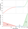 |
Fig. 1. Adopted BD mass distribution in this study; see text for details. |
The normalised histogram values shown in Fig. 1 are simply the first derivative of CDFM(x). In the simulations, the BD mass (MBD) was generated as a random number using the inverse CDF (Appendix F).
Period distribution. Though radial velocity and transit observations are biassed towards the detection of short-period objects, observations show that the number of BDs increases with orbital period, which is consistent with direct imaging surveys (Díaz et al. 2012; Ma & Ge 2014). Because Gaia ’s astrometric sensitivity increases with increasing period up to the mission duration (Appendix A), it is important to have a good representation of the period distribution up to at least the nominal five-year mission length. Most literature data have poor statistics for orbital periods of beyond several years (and are often limited to only 300–500 d), and so we have limited our adopted period distributions to 5 yr.
To satisfy our need to sample beyond more than 1–2 yr, we derived the period distribution from the samples of Ma & Ge (2014) and Díaz et al. (2012) consisting of (partially overlapping) BDs with masses of between 9 and 90 MJ and orbiting solar-type stars with a period shorter than ∼104 d. Unfortunately these studies contain an aggregation of identified objects without the kind of bias sample corrections applied in for example Grether & Lineweaver (2006). Accordingly, their period distributions should probably be used as approximate at best, which is already illustrated by their differences in the cumulative distribution functions (Fig. 2). As we need to represent the longest periods most accurately because they have the highest detectability, we bias our fits towards them. Hereafter, these are referred to as the ‘Ma & Ge’ and ‘Díaz’ fits and are labelled ‘our fit (large P)’ in Fig. 2. For illustration, we also fit the ‘whole’ Díaz et al. (2012) curve with a more complex model (see ‘Díaz our fit (all P)’ in Fig. 2), though the comparison with the histogram seems to suggest such a model does not seem to really represent the underlying distribution better, and it is not used any further for this study. Because the period distribution is amongst the most important factors in determining our predicted numbers, we asses (and combine) the result of both the Ma & Ge and Díaz fits, because they nicely represent two rather different steepnesses of the assumed period distribution towards larger periods.
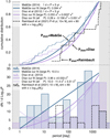 |
Fig. 2. Period distribution of the BD sample from Ma & Ge (2014) and Díaz et al. (2012) which have masses of between 9 and 90 MJ orbiting solar-type stars. Top: cumulative distribution function for BDs. The ‘large P’ fits of Ma & Ge and Díaz are used to generate the BD period distributions and are referred to as Pdistr = Ma & Ge and Pdistr = Díaz, respectively. Bottom figure: log-binned histogram with the corresponding fit curves (bin size log10(1.98)). Our simulations are limited to the indicated (non-shaded) period range 1 d < P< 5 yr. The Raimbault (in prep.) data are used for an additional bootstrap sample estimate (Sect. 5.2). |
In both the Ma & Ge and Díaz fits we set the lower limit to 1 d, based on the apparent cut-off in the population (as these systems should have a high detectability in the radial velocity studies). The lower panel of Fig. 2 suggest that the distributions peak around 2.5–5 yr, though it is unclear whether this could be ascribed to a selection effect in the surveys (due to the survey lengths) or is really a feature of the underlying BD distribution. In the case where a significant population exists with P > 5 yr, Gaia will be able to detect a large fraction of those, especially when the (currently ongoing) ten-year extended mission has been completed.
Period–eccentricity distribution. Ma & Ge (2014) found that there seems to be a statistically significant difference in the distributions of eccentricities for BDs below and above 42.5MJ (the ‘driest’ part of the BD desert). For the BDs with (minimum) masses above 42.5MJ, these latter authors identify the short-period distribution to be consistent with a circularisation limit of ∼12 d, similar to that of nearby stellar binaries (Raghavan et al. 2010). Also, these massive BDs seem to have an apparent absence of eccentricities below e < 0.4 for periods 300 < P < 3000 d, while these eccentricities are populated by BDs with (minimum) masses below 42.5MJ. Additionally, the latter sample suggests a reduction in maximum eccentricity towards higher (minimum) mass, while such a trend seems to be absent in the sample with (minimum) mass above 42.5MJ.
As for the period distribution, we inspect the eccentricity distribution of Ma & Ge (2014) and Díaz et al. (2012) in Fig. 3. Generally, there is not a clear distinction between the lower mass and higher mass regimes in the Ma & Ge (2014) data, and we simply adopt a single fit that allows us to draw eccentricities in the range 0–1 in a continuous fashion. The Díaz et al. (2012) sample has a slightly more eccentric distribution than our fit, though this is in the interval e = 0 − 0.6, for which our detection efficiency varies by only about 10% (Fig. A.1). Accordingly, if the true BD eccentricity distribution follows the Díaz curve, it would have only a marginal effect on the predictions.
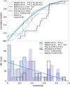 |
Fig. 3. Eccentricity distribution of the BD sample from Ma & Ge (2014) and Díaz et al. (2012). Top: cumulative distribution function for BDs. The ‘Ma & Ge’ fit is used for the simulations in this paper. Bottom figure: binned histogram with the corresponding fit curve (bin size 0.05). Raimbault (in prep.) data are used for an additional bootstrap sample estimate (Sect. 5.2). |
Kipping (2013) suggested that the orbital eccentricity distribution for extrasolar planets is well described by the Beta distribution. We did not perform an extensive fitting, but for illustration we plot the Beta distribution B(2, 4) in Fig. 3, and show the rough mean of the distributions (0.30 for Ma & Ge (2014), and 0.41 for Díaz et al. (2012) for P < 5 yr). This illustrates that there is no good match with Ma & Ge (2014), although the Beta distribution B(2, 4) resembles that found by Díaz et al. (2012) reasonably well. The good fit found for planetary data, B(0.867, 3.03), provides a poor match to these data, heavily under-predicting the observed non-zero eccentricity distribution.
Having chosen our independent distribution functions, we can inspect the period–eccentricity distribution of both Díaz et al. (2012) and Ma & Ge (2014) in Fig. 4. We adopted a circularisation period of Pcirc = 10 d, using the formulation of Halbwachs et al. (2005), as it is an obvious feature in the combined parameter space. We did not adopt a specific mass-dependent eccentricity distribution, in part because the effect is only very marginal in Fig. 3, but also because Grieves et al. (2017) find some new candidates (their Fig. 9) which do not follow the regimes introduced by Ma & Ge (2014), although they do still support a two-population trend.
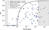 |
Fig. 4. Period–eccentricity distribution of the BD samples from the three sources considered in this study: (1) Ma & Ge (2014) split into low-mass and high-mass samples, (2) Díaz et al. (2012), and (3) that from Raimbault (in prep.) but only for BDs with companions in the 10 − 80 MJ sin i range. In our simulations, a circularisation limit of 10 d is adopted, resulting in the eccentricity limit indicated by the black line. We limit (most of) our derived models to the interval between the shaded areas, namely 1 d < P< 5 yr. |
The way the samples for our simulations are constructed is by first drawing a period from either the Ma & Ge or Díaz period-distribution fit. We then use this period to compute the maximum eccentricity allowed due to the circularisation criterion, and use this to limit the range of the drawing of the eccentricity, effectively cutting the PDF from which we draw the eccentricity from zero to the maximum eccentricity allowed. This means that the effective eccentricity distribution that is used has an increased rate of low-eccentricity systems with respect to the CDF fit-line shown in Fig. 3.
3.3. Host star distribution as observed by Gaia
The number of host stars observed by Gaia as a function of stellar parameters is given by our function Nobs(θ*). This is taken from the Besançon population synthesis model (Robin et al. 2003, 2012a, 2014) for stars with G > 10.5, and is derived from Gaia DR2 data for G < 10.5, as described in Appendices G and H, respectively. The total number of stars brighter than G = 17.5 mag is 130 million. Figure 5 summarises the adopted distribution of host stars, both on the sky, as a function of colour and stellar type, and according to their position in the HR-diagram. The sky distribution of the Gaia data is not shown, but varies between roughly 2 and 6 stars per square degree, with the densest regions in the Galactic plane.
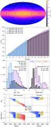 |
Fig. 5. Distribution of the 130 million simulated FGK main sequence (MS) and subgiants (SG) host stars with G < 17.5. Top: logarithmic Galactic sky density (Besançon data only). Second: histogram of G-band counts (bin size: 0.5 mag). Third: Histogram of colour (bin size: 0.1) and type (bin size: 0.2). Bottom: colour–absolute magnitude diagram (Besançon data only). |
Given the adopted constant 0.6% occurrence rate of BDs around any FGK star (Sect. 3.1), we can simulate BD systems for a random sample of the 130 million Besançon and Gaia DR2 stars and scale the resulting counts. For the main results, we simulated a 1% random sample (1.4 million BD systems), scaled by 0.6 to produce the BD counts used to compute the statistics for the first four rows of results in Table 1 and all statistics in Table 2. This sample is referred to as the ‘all magnitudes’ sample hereafter. For the GRVS < 12 selection (see Sect. 4.2), we simulated BD systems on the full set of main sequence and subgiant stars (in our model 1.9 million), and then scaled the simulation counts by 0.006 to get a detailed estimate of the detection rate. This sample was used to compute the statistics from row five onwards in Table 1.
Number of simulated BD detections from Gaia astrometry, radial velocity, and photometric transits.
Throughout this study, we made the assumption that all Gaia and Besançon (host) stars are not in a binary system, apart from the unseen BD component we simulate. The rigorous inclusion of binarity will most likely reduce the number of detectable BDs, as it complicates the modelling. Also, the BD orbital parameter distributions adopted in this paper are likely to be quite different for those orbiting a binary host system.
4. Results
The total number of BDs around Gaia-observable host stars is about 780 000 (listed in the top row of Table 1), which is 0.6% of the 130 million stars with G < 17.5 considered here. Because the number of Gaia detections is highly sensitive to the period distribution, which itself is amongst the most ill-defined priors, we express the final numbers as the range of the counts resulting from two models we derived in Sect. 3.2 (Fig. 2): Pdistr = Ma & Ge and Pdistr = Díaz. Their labels are found in many of the result tables and figures. As seen from Table 1, the Díaz period distribution predicts about 20%–30% more BDs than Ma & Ge (2014). Table 1 allows us to directly draw some overall conclusions: (1) The number of astrometric BDs detectable with Gaia will be in the tens of thousands. (2) The radial velocity time-series for GRVS < 12 will be able to detect about 1000 to 2000 BDs. (3) The total number of stars with detectable BD transits will be about 1000. (4) Stars with both good astrometric and radial velocity BD detections will be in the hundreds. (5) The number of detectable transiting exoplanets in combination with radial velocity detection will be in the tens. (6) Detections of photometric transits together with astrometry (whether including radial velocity or not) will be only a few, and only after an extended ten-year mission.
The sky distribution of solid detections (Δχ2 > 50) of BDs is shown in the second and third panels of Fig. 6, and is ‘weighted’ by the available number of observations shown in the top panel; it can be seen to generally follow the Galactic host-star distribution. The bottom panel shows the detection rates as function of colour, showing that our recovery peaks around GBP − GRP = 0.8 − 0.9. For astrometry, the vast majority of detections (85%) are around main sequence stars, with only 15% coming from subgiants; for radial velocity these values are 65% and 33%, respectively (similar to the ratios in the input data for the bright magnitudes shown in Fig. 5).
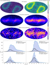 |
Fig. 6. Distributions of the astrometric and radial velocity solid detections (Δχ2 > 50) resulting from the Pdistr = ‘Ma & Ge’ simulation. Top: number of FoV transits for comparison with lower panels. Second: astrometric detections. Third: radial velocity detections. Bottom: histogram of counts as a function of colour (bin size: 0.05), separated by evolutionary stage. |
4.1. Detections by astrometry
For the adopted BD mass range 10 − 80 MJ, we conclude from Table 1 and Fig. 7 that using astrometry alone, Gaia should detect between 41 000 and 50 000 (±23 000) BDs, of which 28 000–34 000 (±15 000) should be reliably detected out to several hundred parsecs with semi-major axis typically in the 0.25 − 2.7 au range. The majority will have P > 200 d, extending up to the five-year adopted upper period limit. Good orbital solutions will be possible for about 17 000–21 000 (±10 000) systems. We note that the detection sensitivity for short astrometric periods P ≲ 100 days is rather non-uniform; see Appendix A.
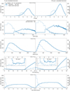 |
Fig. 7. Histograms of the astrometric and radial velocity solid detections (Δχ2 > 50) resulting from the Pdistr = ‘Ma&Ge’ simulation. Top panel: host star magnitude. Second panel: period. Third panel: distance. Fourth panel: BD mass. Bottom panel: semi-major axis |

In Fig. 7 we see that the distribution peaks around G ∼ 14 − 15 where the stellar number density (Fig. 5) and still relatively small astrometric error (Fig. C.1) produce the highest gain. Figure 7 also shows the majority of recoveries are for the more massive BDs, as expected from Eq. (1). We note that even though we depleted the mass-prior distribution of the ‘desert’ region to contain only 2% of the simulated BDs, there are still tens of confident detections.
Figure 8 shows the distributions as a function of magnitude for all detection thresholds of the various parameters. The bottom panel shows that the detection fraction (completeness) steadily increases towards the bright end, though for the most populated magnitudes it reaches only 10%–30%. For a ten-year mission, this number rises to 20%–40%, and the mode of the distribution is extended by about 0.3 mag and 20%–30% in distance.
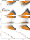 |
Fig. 8. Distributions of the BDs resulting from the five-year (left) and ten-year (right) Gaia simulations using Pdistr = Ma & Ge for the three adopted astrometric detection thresholds: Δχ2 > 30 (41 000, 64 000), Δχ2 > 50 (28 000, 45 000), and Δχ2 > 100 (17 000, 28 000). (The point-cloud data are from 1% simulations (Sect. 3.3), hence scale by 0.6 to get the BD rates of Table 1.) |
For the G > 10.5 Besançon model data (not plotted), we have the detailed type information available, telling us that for the solid detections, 40% are G-type host stars, 32% are host K-stars, and 28% are host F-stars. The recovery numbers are declining at the edges of our adopted range of stellar types, that is, towards the more massive F-stars and less-massive K-stars, confirming the assumption outlined in Sect. 1 that the majority of BD detections are expected around FGK-stars.
4.2. Detections by radial velocity
Here we discuss only sources with Gaia radial velocity time-series selected by GRVS < 12 (G ⪅ 12.7). From Table 1, we see that we can expect 1700–1300 (±800) BD detections from Gaia radial velocity measurements, of which 1100–830 (±500) will be robust, and 570–410 (±250) with good orbital parameters. As expected, the largest numbers are found at short orbital periods and for the most massive BDs (55 − 80 MJ; see Figs. 7 and 9), although several tens of those will extend to the lowest BD masses. The largest number of detections is around G = 11 − 12, where the detection fraction is around 30%–60%. A ten-year mission boosts this to 40%–70%.
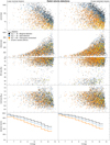 |
Fig. 9. Same as Fig. 8 but now for the three adopted Gaia radial velocity detection thresholds (i.e. limited to stars with GRVS < 12): Δχ2 > 30 (1700, 2700), Δχ2 > 50 (1100, 1900), and Δχ2 > 100 (570, 1100). (The point-cloud data are from 1% simulations (Sect. 3.3), hence scale by 0.6 to get the BD rates of Table 1.) |
Fig. 7 shows the distance limit is a few hundred parsecs at maximum with a semi-major axis of typically below 0.25 au. Mainly periods below 10 d are recovered, and therefore the eccentricity distribution (not shown) is peaking at zero due to the adopted eccentricity limit (which is zero for periods below 10 d; see Fig. 3). Recovery as a function of inclination (not shown) is roughly limited to the range of 20° < i < 160° and is rather flat in the range of 60° < i < 120°, as expected from Eq. (2) and the random orientation input distribution.
The combination of astrometric and radial velocity detections (i.e. the last three rows of Table 1 and shown in Fig. 10) yields 810–750 (±400) systems, of which 410–370 (±200) have good orbital solutions from either data set. This will be an important sample, because a joint solution would better constrain all system parameters. Additionally, as all sources with Gaia RV time-series are relatively bright, this set will be ideal for follow-up observations. Most noticeable is that the number of systems in this sample doubles for an extended mission of 10 yr.
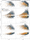 |
Fig. 10. Intersection of Figs. 8 and 9, i.e. where the same detection threshold is passed for both Gaia astrometry and radial velocity (hence limited to stars with GRVS < 12): Δχ2 > 30 (810, 1600), Δχ2 > 50 (410, 950), and Δχ2 > 100 (140, 400). (The point-cloud data are from 1% simulations (Sect. 3.3), hence scale by 0.6 to get the BD rates of Table 1.) |
4.3. Detections by photometric transits
For each simulation, we list the number of sources that have at least three detectable transits (S/N > 3) in parenthesis in Tables 1 and 3, together with their average number of observations in transit. The transit depth and period distribution of the Ma & Ge five-year sample are shown in Fig. 11.
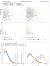 |
Fig. 11. Transit statistics from the Pdistr = Ma & Ge simulation for a five-year and ten-year mission of 1.5 million randomly oriented BDs. These BD number counts are scaled by 0.6 to represent a 0.6% BD occurrence rate in Table 1; see Sect. 3.3. Detailed period-binned statistics of the ‘ALL’ part are shown in Table 2. |
As seen from the top row of Table 1, detectable photometric transits are expected for some 720–1100 (±450) mainly short-period BDs with periods mainly below 10 d (Fig. 11), each yielding around four to five transits on average. Direct identification of these objects as BDs would be difficult from the Gaia photometry alone, but this would yield a very interesting follow-up sample.
For GRVS < 12, this number drops to 34–53 BDs each with typically five observable transits. Because both radial velocity and photometric transit detection methods are sensitive to large orbital inclination and short orbital period, out of this small sample, about one-half should be detectable with both methods, growing to perhaps 40–60 BDs for a ten-year mission.
For astrometrically detectable BDs with at least three detectable photometric transits, the numbers remain below double figures, and drop to almost zero below GRVS < 12 (whether or not we check for coincidence with radial velocity detection). A ten-year mission could yield at most a few of these ‘triple method’ detections.
Let us go into more detail for a moment. The largest main sequence stars4 have diameters of around 1.79 R⊙ (F0V) and the smallest around 0.65 R⊙ (K9V). For an adopted BD radius of RJ ∼ 0.1 R⊙, this means that the predicted transit depth (RBD/R*)2 ranges between 0.3% and 2.3%, corresponding to Δm ≃ 3 − 25 mmag. This is around the Gaia noise limit (see Appendix E) for most of the considered magnitude range and using a threshold of S/N > 3 causes a drop of a factor 3–4 in detected number of sources with at least one observable transit (not shown). In Table 2, we list the total transit statistics for the ‘all magnitudes’ simulation sample (described in Sect. 3.3) using Pdistr = Ma & Ge for different period bins. When only requiring at least one transit with S/N > 3 (left column): for a five-year simulation 64–128 day bin, we can see that of all observations of all randomly oriented sources, there is 1 in 56 000 observations in transit ( ), and 1 in 1100 sources that have non-zero transits (
 ). For those sources that have non-zero transits, the mean number of transits is
  . When we select a minimum number of three transits with S/N > 3 on the photometric transits (as we demand in this study), the source occurrence rates of all period bins drop by a significant factor of 2.5 to 8. For a ten-year mission, the fraction of observations in transit does not change significantly (as this is mainly due to the inclination of the systems), but the number of sources with transits is increasing by up to a factor of 2 for the longer periods, though hardly changes for those with short orbital periods, as they were likely to transit already within the five years of data collection. For a ten-year mission, the average number of transits per source increases by up to a factor of 1.5 with the largest increase mainly for the short-period objects as expected.
Simulated BD photometric transit statistics as a function of period bin.
In the Ma & Ge five-year and ten-year transit ‘ALL’ sample shown in Fig. 11, 71% of the identified transiting systems are around main sequence stars, reflecting the simulated input distribution.
5. Discussion
5.1. Comparison with earlier work
Bouchy (2014) found that some 20 000 astrometric BD detections could be expected for bright GRVS < 12 host stars with radial velocity time-series in Gaia, assuming they have: a 0.6% BD occurrence rate (as assumed in this paper), 3.4 million main sequence and subgiants stars (total count from Robin et al. 2012b for these luminosity classes), and a 100% detection efficiency.
As seen in Fig. 4.2, applying the limit of GRVS < 12 results in a sample of 1.8 million stars, which is only about half of those assumed in Bouchy (2014). The difference is that in the latter, the selection is not constrained to only FGK stars5. In Robin et al. (2012b), the fraction of FGK stars with GRVS < 12 is 71% (20% larger than expected from the discrepancy), though this is not limited to the aforementioned luminosity classes.
As mentioned in Sect. 4.1, we find around 5000 BDs with a detection efficiency of about 30%−50% (see Fig. 8 around G 11–12.5). Comparing this with the 100% detection efficiency assumed in Bouchy (2014), we can explain the discrepancy between their 20 000 and our ∼5000 BDs: our sample is about half as large, and has a detection fraction that is also half as large. Given that Bouchy (2014) did not constrain their estimate to FGK host stars, their BD number could be overestimated by a factor 2 when only considering the astrometric detection probability (which is closer to 50% than 100%). Bouchy (2014) also predicted a total of 60 transiting BDs for GRVS < 12, which is almost in line with the 35–50 BDs we predict in Table 1.
Sozzetti (2014a) made an order-of-magnitude estimate of thousands of BD companions with G < 16 mag that can be astrometrically detected using their 3-sigma criterion, which is in line with the findings of this study. Perryman (2018, Sect. 2.10.5) considered many tens of thousands of BDs to be detected in total, which matches our predictions.
The most deviating prediction of several tens of BDs detectable by astrometry mentioned in Andrews et al. (2019) seems to be explained by the detection criterion used: it focussed on tightly constraining the mass function, which requires more signal than a detection or even a well-constrained orbital fit. A small investigation where we attempted to reproduce their results indicated that a well-constrained mass function corresponds to a Δχ2 of several thousand or more, i.e. it is much more stringent and thus will lead to (much) more conservative rate estimates.
5.2. Estimates from a uniformly sampled data set
In an attempt to estimate the number of expected BDs from a uniformly sampled dataset, we used the Coralie survey dataset of Raimbault (in prep.) which contains about 100 targets with companions of 2 < MJ sin i < 433 for a volume limited sample. Seventeen of these targets have 10 < MJ sin i < 80, of which two have P ∼ 6 yr and one has P ∼ 10 yr. As the latter will be hard to detect, we remove it from the sample, but keep the two six-year entries, that is, a total sample of 16 BDs. We run an additional simulation with this sample, but instead of sampling the companion mass, eccentricity, period, and period–eccentricity from our adopted CDF distributions, we bootstrap all our candidates from this sample (drawing samples with replacement). The comparison between the CDFs is illustrated in Figs. 2–4, showing that the Raimbault (in prep.) distribution differs significantly from those derived from the Ma & Ge (2014) and Díaz et al. (2012) data.
We note that we simply use MJ sin i as a proxy for MJ. The results are shown in Table 3, indicating that the estimates would be 1.5–2 times higher than that using our adopted distributions (Table 1). Given that we adopted the minimum mass estimate in our simulations, and the Gaia sensitivity is higher for more massive companions, this might suggest that if the Raimbault sample is representative for the real BD distribution, we could expect up to twice as many BDs as suggested in Table 1.
Simulation results from bootstrapping with a BD sample from Raimbault (in prep.).
6. Conclusions
Based on detailed simulations, we find that Gaia is likely to detect tens of thousands of BDs from the astrometric data alone. From the Gaia radial velocity data alone, there should be between 1000 and 2000 additional candidates, with a few hundred overlapping in the two domains. Systems with at least three photometric transits with S/N > 3 are expected for perhaps 1000 systems, which would be excellent targets for follow up. Among these, a few tens of systems overlap with radial velocity detections and a few (at most) overlap with astrometric detections. An extended mission of 10 yr increases all of the detected numbers by 50%–200%, allowing the BD horizon to be extended significantly.
The numbers found in this study are ultimately limited in accuracy to about ±50% due to the present uncertain occurrence rates and period distributions of BDs around the considered FGK host stars. However, what is certain is that the Gaia detections will enlarge the current BD sample by at least two orders of magnitude, allowing the BD fraction and orbital architectures to be investigated as a function of host stellar parameters in greater detail than every before, leading to a better understanding of the formation scenarios of these substellar companions to FGK dwarfs and subgiants that populate the 10 − 80 MJ mass range, and the exploration of the (perhaps not completely dry) desert within it.
We note that epoch radial velocities will only be published for sources with GRVS ≤ 12 − 13 mag; for fainter sources only mean radial velocities will be published.
Though some computational cost is involved in simulating the orbital signal of a Keplerian system and making a 5-parameter solution to it, it is much cheaper than taking the average of a large number of Keplerian 12-parameter solutions to Monte Carlo noise realisations of the same signal, while providing almost the same information.
An exception to this are systems with an orbital period very close to the one-year parallactic motion; see Lattanzi et al. (2000), Butkevich (2018), Sozzetti et al. (2010) for more detailed discussions.
Using radii from reference in footnote 12.
We tried to extract the sample size of the FGK main sequence and subgiant with GRVS < 12 from the Robin et al. (2012b) catalogue on Vizier, but unfortunately it does not contain the luminosity class.
For completeness we wish to convey that the astrometric sensitivity of Gaia to detect unseen companions has been assessed in various works in the literature (see e.g. Casertano et al. 2008; Sozzetti 2010a,a, 2014b,a) using the per-transit ‘S/N statistic’ which compares the astrometric signature (Eq. 1) of the host star against the (typical) accuracy of an individual epoch, σfov, astro.
From Julian year 2014.734 (2014-09-26, start of Nominal Scanning Law phase) to 2019.734 (2019-09-26) for the nominal 5-year mission, and up to 2024.734 (2024-09-25) for the 10-yr extension.
This traced in a rough way the orange mode-line of the distribution in Fig. 9 of Evans et al. (2018), and is rescaled to represent the corresponding precision per FoV (in absence of any noise floor). We note that meanCcdPerFov represents the number: 8.857 = (6/7*9+1/7*8), i.e. the focal plane has seven rows of CCDs of which one has eight CCDs and the others have nine CCDs that are used to derive G-band photometry.
We query a random sample of photometry of 1M EDR3 sources (Riello et al. 2021) with a minimum of 150 CCD observations (phot_g_n_obs) and directly scale them to the (noise-floor free) per-FoV precision in magnitude: fov_uncertainty_mag= 1.0857/sqrt((6/7*9+1/7*8))*phot_g_mean_flux_error *sqrt(phot_g_n_obs)/ phot_g_mean_flux.
This coincides with the pre-launch estimate of 1 mmag adopted by Dzigan & Zucker (2012). At that time it was assumed this floor would extend to G = 14 or beyond, such that their predicted transit counts fainter than 14 mag should be considered as somewhat optimistic.
V2019.3.22 (Eric Mamajek) of http://www.pas.rochester.edu/~emamajek/EEM_dwarf_UBVIJHK_colors_Teff.txt
r_est from: http://gaia.ari.uni-heidelberg.de/tap.html
Acknowledgments
We acknowledge financial support from the Swiss National Science Foundation (SNSF). This work has, in part, been carried out within the framework of the National Centre for Competence in Research PlanetS supported by SNSF. LL is supported by the Swedish National Space Board. We would like to thank the referee Alessandro Sozzetti for his detailed remarks and suggestions that much improved the quality and relevance of this paper. Thanks also to Lorenzo Rimoldini, Jeff Andrews, Danley Hsu, Laurent Eyer, Johannes Sahlmann and Céline Reylé for helpful feedback on specific aspects of this paper. Thanks to David Katz for discussion on the per-FoV radial velocity error model and Shay Zucker for discussion on a useful photometric transit detection criterion. This work has made use of data from the European Space Agency (ESA) mission Gaia (https://www.cosmos.esa.int/gaia), processed by the Gaia Data Processing and Analysis Consortium (DPAC, https://www.cosmos.esa.int/web/gaia/dpac/consortium). Funding for the DPAC has been provided by national institutions, in particular the institutions participating in the Gaia Multilateral Agreement.
References
- Andrae, R., Fouesneau, M., Creevey, O., et al. 2018, A&A, 616, A8 [NASA ADS] [CrossRef] [EDP Sciences] [Google Scholar]
- Andrews, J. J., Breivik, K., & Chatterjee, S. 2019, ApJ, 886, 68 [NASA ADS] [CrossRef] [Google Scholar]
- Arenou, F., Luri, X., Babusiaux, C., et al. 2018, A&A, 616, A17 [NASA ADS] [CrossRef] [EDP Sciences] [Google Scholar]
- Bailer-Jones, C. A. L., Rybizki, J., Fouesneau, M., Mantelet, G., & Andrae, R. 2018, AJ, 156, 58 [Google Scholar]
- Borgniet, S., Lagrange, A. M., Meunier, N., & Galland, F. 2017, A&A, 599, A57 [NASA ADS] [CrossRef] [EDP Sciences] [Google Scholar]
- Borucki, W. J., Koch, D., Basri, G., et al. 2010, Science, 327, 977 [Google Scholar]
- Bouchy, F. 2014, Mem. Soc. Astron. It., 85, 665 [NASA ADS] [Google Scholar]
- Bouchy, F., Ségransan, D., Díaz, R. F., et al. 2016, A&A, 585, A46 [NASA ADS] [CrossRef] [EDP Sciences] [Google Scholar]
- Butkevich, A. G. 2018, MNRAS, 476, 5658 [NASA ADS] [CrossRef] [Google Scholar]
- Casertano, S., Lattanzi, M. G., Sozzetti, A., et al. 2008, A&A, 482, 699 [NASA ADS] [CrossRef] [EDP Sciences] [Google Scholar]
- Chabrier, G., Johansen, A., Janson, M., & Rafikov, R. 2014, Protostars and Planets VI, eds. H. Beuther, R. S. Klessen, C. P. Dullemond, & T. Henning, 619 [Google Scholar]
- Cropper, M., Katz, D., Sartoretti, P., et al. 2018, A&A, 616, A5 [NASA ADS] [CrossRef] [EDP Sciences] [Google Scholar]
- Czekaj, M. A., Robin, A. C., Figueras, F., Luri, X., & Haywood, M. 2014, A&A, 564, A102 [NASA ADS] [CrossRef] [EDP Sciences] [Google Scholar]
- de Bruijne, J. H. J. 2014, ArXiv e-prints [arXiv:1404.3896] [Google Scholar]
- Díaz, R. F. 2018, in Asteroseismology and Exoplanets: Listening to the Stars and Searching for New Worlds, 49, 199 [CrossRef] [Google Scholar]
- Díaz, R. F., Santerne, A., Sahlmann, J., et al. 2012, A&A, 538, A113 [NASA ADS] [CrossRef] [EDP Sciences] [Google Scholar]
- Duquennoy, A., & Mayor, M. 1991, A&A, 500, 337 [NASA ADS] [Google Scholar]
- Dzigan, Y., & Zucker, S. 2012, ApJ, 753, L1 [NASA ADS] [CrossRef] [Google Scholar]
- Evans, D. W., Riello, M., De Angeli, F., et al. 2018, A&A, 616, A4 [NASA ADS] [CrossRef] [EDP Sciences] [Google Scholar]
- Faherty, J. K., Gagné, J., Burgasser, A. J., et al. 2018, ApJ, 868, 44 [Google Scholar]
- Figueira, P. 2018, in Asteroseismology and Exoplanets: Listening to the Stars and Searching for New Worlds, 49, 181 [NASA ADS] [CrossRef] [Google Scholar]
- Gaia Collaboration (Prusti, T., et al.) 2016a, A&A, 595, A1 [NASA ADS] [CrossRef] [EDP Sciences] [Google Scholar]
- Gaia Collaboration (Brown, A. G. A., et al.) 2016b, A&A, 595, A2 [NASA ADS] [CrossRef] [EDP Sciences] [Google Scholar]
- Gaia Collaboration (Brown, A. G. A., et al.) 2018, A&A, 616, A1 [NASA ADS] [CrossRef] [EDP Sciences] [Google Scholar]
- Gaia Collaboration (Brown, A. G. A., et al.) 2021, A&A, 649, A1 [NASA ADS] [CrossRef] [EDP Sciences] [Google Scholar]
- Górski, K. M., Hivon, E., Banday, A. J., et al. 2005, ApJ, 622, 759 [Google Scholar]
- Grether, D., & Lineweaver, C. H. 2006, ApJ, 640, 1051 [Google Scholar]
- Grieves, N., Ge, J., Thomas, N., et al. 2017, MNRAS, 467, 4264 [Google Scholar]
- Halbwachs, J. L., Mayor, M., & Udry, S. 2005, A&A, 431, 1129 [NASA ADS] [CrossRef] [EDP Sciences] [Google Scholar]
- Hatzes, A. P. 2016, in Methods of Detecting Exoplanets: 1st Advanced School on Exoplanet Science, eds. V. Bozza, L. Mancini, & A. Sozzetti, 428, 3 [NASA ADS] [CrossRef] [Google Scholar]
- Holl, B., Lindegren, L., & Hobbs, D. 2012, A&A, 543, A15 [NASA ADS] [CrossRef] [EDP Sciences] [Google Scholar]
- Holl, B., Audard, M., Nienartowicz, K., et al. 2018, A&A, 618, A30 [NASA ADS] [CrossRef] [EDP Sciences] [Google Scholar]
- Hsu, D. C., Ford, E. B., Ragozzine, D., & Ashby, K. 2019, AJ, 158, 109 [NASA ADS] [CrossRef] [Google Scholar]
- Jordi, C., Høg, E., Brown, A. G. A., et al. 2006, MNRAS, 367, 290 [NASA ADS] [CrossRef] [Google Scholar]
- Jordi, C., Gebran, M., Carrasco, J. M., et al. 2010, A&A, 523, A48 [NASA ADS] [CrossRef] [EDP Sciences] [Google Scholar]
- Katz, D., Sartoretti, P., Cropper, M., et al. 2019, A&A, 622, A205 [NASA ADS] [CrossRef] [EDP Sciences] [Google Scholar]
- Kiefer, F., Hébrard, G., Sahlmann, J., et al. 2019, A&A, 631, A125 [NASA ADS] [CrossRef] [EDP Sciences] [Google Scholar]
- Kipping, D. M. 2013, MNRAS, 434, L51 [Google Scholar]
- Lammers, U., Lindegren, L., Bombrun, A., O’Mullane, W., & Hobbs, D. 2010, in Astronomical Data Analysis Software and Systems XIX, eds. Y. Mizumoto, K. I. Morita, & M. Ohishi, ASP Conf. Ser., 434, 309 [NASA ADS] [Google Scholar]
- Lattanzi, M. G., Sozzetti, A., & Spagna, A. 2000, in From Extrasolar Planets toCosmology: The VLT Opening Symposium eds. J. Bergeron, & A. Renzini, 479 [CrossRef] [Google Scholar]
- Lindegren, L., Lammers, U., Hobbs, D., et al. 2012, A&A, 538, A78 [NASA ADS] [CrossRef] [EDP Sciences] [Google Scholar]
- Lindegren, L., Lammers, U., Bastian, U., et al. 2016, A&A, 595, A4 [NASA ADS] [CrossRef] [EDP Sciences] [Google Scholar]
- Lindegren, L., Hernández, J., Bombrun, A., et al. 2018, A&A, 616, A2 [NASA ADS] [CrossRef] [EDP Sciences] [Google Scholar]
- Lindegren, L., Klioner, S. A., Hernández, J., et al. 2021, A&A, 649, A2 [EDP Sciences] [Google Scholar]
- Ma, B., & Ge, J. 2014, MNRAS, 439, 2781 [Google Scholar]
- Marcy, G. W., & Butler, R. P. 2000, PASP, 112, 137 [Google Scholar]
- Marshall, D. J., Robin, A. C., Reylé, C., Schultheis, M., & Picaud, S. 2006, A&A, 453, 635 [NASA ADS] [CrossRef] [EDP Sciences] [Google Scholar]
- O’Mullane, W., Lammers, U., Lindegren, L., Hernandez, J., & Hobbs, D. 2011, Exp. Astron., 31, 215 [CrossRef] [Google Scholar]
- Oshagh, M. 2018, Asteroseismology and Exoplanets: Listening to the Stars and Searching for New Worlds, 49, 239 [NASA ADS] [CrossRef] [Google Scholar]
- Pecaut, M. J., & Mamajek, E. E. 2013, ApJS, 208, 9 [Google Scholar]
- Perryman, M. 2018, The Exoplanet Handbook, 2nd edn. (Cambridge, UK: Cambridge University Press) [Google Scholar]
- Perryman, M. A. C., de Boer, K. S., Gilmore, G., et al. 2001, A&A, 369, 339 [NASA ADS] [CrossRef] [EDP Sciences] [Google Scholar]
- Perryman, M., Hartman, J., Bakos, G. Á., & Lindegren, L. 2014, ApJ, 797, 14 [Google Scholar]
- Raghavan, D., McAlister, H. A., Henry, T. J., et al. 2010, ApJS, 190, 1 [Google Scholar]
- Ranalli, P., Hobbs, D., & Lindegren, L. 2018, A&A, 614, A30 [NASA ADS] [CrossRef] [EDP Sciences] [Google Scholar]
- Reylé, C. 2018, A&A, 619, L8 [NASA ADS] [CrossRef] [EDP Sciences] [Google Scholar]
- Riello, M., De Angeli, F., Evans, D. W., et al. 2018, A&A, 616, A3 [NASA ADS] [CrossRef] [EDP Sciences] [Google Scholar]
- Riello, M., De Angeli, F., Evans, D. W., et al. 2021, A&A, 649, A3 [NASA ADS] [CrossRef] [EDP Sciences] [Google Scholar]
- Risquez, D., van Leeuwen, F., & Brown, A. G. A. 2013, A&A, 551, A19 [NASA ADS] [CrossRef] [EDP Sciences] [Google Scholar]
- Robin, A. C., Reylé, C., Derrière, S., & Picaud, S. 2003, A&A, 409, 523 [NASA ADS] [CrossRef] [EDP Sciences] [Google Scholar]
- Robin, A. C., Marshall, D. J., Schultheis, M., & Reylé, C. 2012a, A&A, 538, A106 [NASA ADS] [CrossRef] [EDP Sciences] [Google Scholar]
- Robin, A. C., Luri, X., Reylé, C., et al. 2012b, A&A, 543, A100 [NASA ADS] [CrossRef] [EDP Sciences] [Google Scholar]
- Robin, A. C., Reylé, C., Fliri, J., et al. 2014, A&A, 569, A13 [CrossRef] [EDP Sciences] [Google Scholar]
- Sahlmann, J., Ségransan, D., Queloz, D., et al. 2011, A&A, 525, A95 [NASA ADS] [CrossRef] [EDP Sciences] [Google Scholar]
- Sahlmann, J., Triaud, A. H. M. J., & Martin, D. V. 2015, MNRAS, 447, 287 [NASA ADS] [CrossRef] [Google Scholar]
- Santerne, A., Moutou, C., Tsantaki, M., et al. 2016, A&A, 587, A64 [NASA ADS] [CrossRef] [EDP Sciences] [Google Scholar]
- Santos, N. C., Israelian, G., & Mayor, M. 2001, A&A, 373, 1019 [NASA ADS] [CrossRef] [EDP Sciences] [Google Scholar]
- Sarro, L. M., Berihuete, A., Carrión, C., et al. 2013, A&A, 550, A44 [NASA ADS] [CrossRef] [EDP Sciences] [Google Scholar]
- Sartoretti, P., Katz, D., Cropper, M., et al. 2018, A&A, 616, A6 [NASA ADS] [CrossRef] [EDP Sciences] [Google Scholar]
- Sozzetti, A. 2010a, EAS Pub. Ser., 45, 273 [NASA ADS] [CrossRef] [EDP Sciences] [Google Scholar]
- Sozzetti, A. 2010a, in EAS Publications Series, eds. K. Gożdziewski, A. Niedzielski, & J. Schneider, EAS Pub. Ser., 42, 55 [NASA ADS] [CrossRef] [EDP Sciences] [Google Scholar]
- Sozzetti, A. 2014a, Mem. Soc. Astron. It., 85, 643 [NASA ADS] [Google Scholar]
- Sozzetti, A. 2014b, EAS Pub. Ser., 67–68, 93 [CrossRef] [EDP Sciences] [Google Scholar]
- Sozzetti, A., & Desidera, S. 2010, A&A, 509, A103 [NASA ADS] [CrossRef] [EDP Sciences] [Google Scholar]
- Sozzetti, A., Giacobbe, P., Lattanzi, M. G., et al. 2014, MNRAS, 437, 497 [NASA ADS] [CrossRef] [Google Scholar]
- Sozzetti, A., Latham, D. W., Torres, G., et al. 2010, in Chemical Abundances in the Universe: Connecting First Stars to Planets, eds. K. Cunha, M. Spite, & B. Barbuy, 265, 416 [NASA ADS] [Google Scholar]
- Tokovinin, A. A. 1992, A&A, 256, 121 [NASA ADS] [Google Scholar]
- Troup, N. W., Nidever, D. L., De Lee, N., et al. 2016, AJ, 151, 85 [NASA ADS] [CrossRef] [Google Scholar]
- Wilson, P. A., Hébrard, G., Santos, N. C., et al. 2016, A&A, 588, A144 [NASA ADS] [CrossRef] [EDP Sciences] [Google Scholar]
Appendix A: Astrometric and radial velocity detection limits
This section is intended to provide insight into the astrometric and radial velocity detection limits by means of simulating a large grid of models for unseen companions. We note that these data were not used in any of the computations of this paper, and simply serve as illustration for the reader6. Though this paper focuses on the BD mass range, the method is applicable to unseen companions of any mass, such as neutron stars, white dwarfs, and black holes.
The Gaia astrometric and radial velocity detection limits of a specific binary companion depend on the time sampling (Appendix B) and error models (Appendices C and D). Provided with these, we can construct the detection limits as a function of the companion orbital parameters. Below we detail the resulting behaviour.
A.1. Simulating detection limits
For a given host mass (M* in M⊙), absolute magnitude ( ), companion mass (MBD), eccentricity (e), period (P in days), and distance (d in pc), we make 2 × 784 simulations: for 784 HEALPix sky-uniform distributed time-series (see Appendix B) we sample the time series for both a five-year and ten-year mission, with each observation being subject to a random rejection probability of ∼10% to simulate dead time.
The reference time for the astrometric model, tref, is set to the middle of the selected time-series. From the parallax (ϖ in arcsec = 1/distance in pc) and  we compute the apparent G-band magnitude of the host star assuming zero extinction:
  , which is used to extract the astrometric error on the observations using Eq. C.1.
The companion-to-host semi-major axis ( in au) is computed from the period and sum of the masses using Kepler’s third law:
  . The sky-projected semi-major axis (a* in arcsec) of the host star with respect to the system barycentre is computed from
  , the parallax, and mass ratio (q = MBD/M*) as:
  . The orientation of the companion is randomly drawn in 3D space, i.e. inclination, argument of periapsis, position angle of the receding node, and mean anomaly at tref. For each astrometric simulation, the centrality parameter λ (Sect. 2.1) is computed.
In a next step, for the five- and ten-year simulations separately, we compute the fraction of the 768 simulations for which λ > 23, 43, 93, i.e. the fraction of simulations corresponding to the Δχ2 > 30, 50, 100 astrometric detection thresholds. The 768 simulations uniformly cover the whole sky and each have a random orbit orientation; this fraction can therefore be considered a ‘sky average’ value.
The radial velocity detection limits are computed in the same way using the radial velocity centrality parameter λ (Sect. 2.2) and the λ > 25, 45, 95 thresholds corresponding to the Δχ2 > 30, 50, 100 radial velocity detection thresholds. The RVS magnitude is approximated as: GRVS = G + 0.65 for all three stellar types. We note that due to the random orientation of the systems in the simulation, the radial velocity limits will represent detection limits for a ‘typical’ average inclination of 60°.
Originally, we intended to tabulate a comprehensive list of detection curve data for use by the community. Due to the strong dependency on host type (mass and absolute magnitude), relevant companion masses (which can be of any-mass unseen companion), and orbital parameters (mainly eccentricity and inclination), this table would become very large and might still not cover the specific needs of certain potential users. We therefore suggest that anyone interested in using our detection limits should either implement the different accuracy models and computation methods, or contact the main author of this paper to request specific detection curves of interest.
A.2. Interpreting detection limits
To plot the response as a function of period (or semi-major axis) as shown in Figs. A.1 and A.2, we compute these statistics for a range of logarithmically increasing distances and identify (interpolate) the distance of the 10%, 50%, and 90% sky-detection fraction of the various λ thresholds.
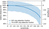 |
Fig. A.1. Astrometric eccentricity dependence of distance and magnitude detection limits for Δχ2 = 100 for a G2V star and a 10 MJ BD with P = 4 yr. The black point at e = 0 corresponds to the black point in the middle panel of Fig. A.2. Sky-detection fractions of 50 percentile (thick line) and 10–90 percentile (shaded region) illustrate that the detection threshold for such a (randomly oriented) system varies by ±25%, depending on sky position. |
We start by describing the astrometric detection limits. The results of the astrometric 50% sky recovery fraction is shown by the lines in Figs. A.1 and A.2, while the 10% and 90% fractions are used to draw the shaded range in Fig. A.1. For example, the black dot in both figures is a BD companion around a G2V star (1 M⊙) with a zero eccentricity BD of mass 10 MJ, having P = 4 yr, observed during a five-year nominal mission. It will have a good orbit recovery (Δχ2 = 100) for 50% of the sky at 311 pc. The distance range corresponding to the 10% and 90% sky coverage for this recovery is 381–234 pc, i.e. ± ∼ 25% visualised by the shaded range at eccentricity zero of Fig. A.1. As eccentricity increases, the detection efficiency slowly decreases, resulting in a distance limit of about 10% lower around e = 0.5, and reaching more than 20% lower for e > 0.7. Given the significant eccentric distribution of BDs (see Sect. 3.2), the overall effect is non-negligible. The solid line is similar for other periods of this system, though the 10%–90% sky coverage range increases for shorter periods: e.g. to ±45% for P = 1 yr. Comparing this to a 100 MJ companion, the 50% sky fraction solid line drops below 20% for e > 0.8, while the 10%–90% sky coverage range expands from ±15% to some ±25% for P = 4 to P = 1 yr.
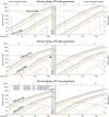 |
Fig. A.2. Illustration of the Gaia astrometric and radial velocity detection limits for the adopted BD mass range 10– 80 MJ around a F0V/G2V/K6V main sequence star (top/middle/bottom respectively) for different Δχ2 detection thresholds (see Sect. 2.1) resulting from a simulated five-year nominal mission (left) and ten-year extended mission (right). For each Δχ2 detection threshold, the lines show for a given period (bottom axis) and semi-major axis (top axis), the zero-extinction limits in distance (left axis) and apparent G-band magnitude (right-axis) for which 50% of the simulated sky positions are no longer detectable. The ascending thick lines are the astrometric limits, while the descending thin lines are the radial velocity limits. We note that the latter are truncated due to the GRVS = 12 limit (see text for details). For the dot in the middle panel, the astrometric eccentricity dependence and sky-position variation is expanded in Fig. A.1; see Sect. A for more details. For comparison, in grey we include the astrometric detection thresholds for a 1 MJ planet (it is not detectable using Gaia radial velocity). |
Fig. A.2 demonstrates that detectability increases for increasing period, which can be understood through Kepler’s third law: the (projected) semi-major axis increases as a function of period, which boosts detectability. The peak occurs around the mission length, and as discussed in Sect. 2.1, periods (much) beyond the mission length are increasingly difficult to recover, and good parameter recovery is no longer connected to the adopted Δχ2 > 100. To make this clear, this region is shaded in the plots.
The adopted astrometric accuracy floor for G < 12 (see Fig. C.1 of Appendix C) leads to a different slope of the detectability curves of Fig. A.2 for distance < 800, < 300, and < 85 pc, for the shown F0V, G2V, and K6V host star, respectively. Thus, for the G < 12 regime the difference in detectability between host stars is only dependent on q, which for a given MBD is higher for late-type stars. As the detectability of a 1 MJ companion lies within the G < 12 regime, this translates into the further distance limit for the 1 MJ companions for a K6V host compared to a F0V host, as seen in Fig. A.2.
For parts of the curves that are in the G>( ≫ )12 regime, the astrometric error is strongly dependent on apparent magnitude (Fig. C.1), which effectively ‘outweighs’ the smaller mass ratio for heavier stellar host mass, and hence produces a larger astrometric signal for earlier type stars, e.g. as seen in the further distance limit of the peak of a 100 MJ companion for a F0V star compared to a K6V.
In summary, for the astrometric detection limits: (1) for a given host and BD mass, the detectability increases with period and reaches maximum sensitivity for periods close to the mission length; (2) orbital parameters of systems with periods (well) beyond the mission length are not recovered; (3) increased eccentricity reduces detectability; (4) for a given companion mass, companions around earlier type stars are detectable at larger distances when G > 12 due to the higher intrinsic brightness of the host star and the specific Gaia magnitude-dependent accuracy, despite the smaller mass ratio.
A particular feature of the Gaia astrometric data sampling is that the detection sensitivity for short astrometric periods P ≲ 100 days is highly non-uniform and gives rise to a rather complex variation of detectability as a function of sky position (i.e. time-sampling) and orbital parameters (mainly related to the sky orientation of the orbit). Even though Fig. A.2 provides sky and orbit averaged values along its lines, the effect is still mildly visible in the wiggles of the lines. An alternative illustration of this effect can be found in Fig. 5 of Sozzetti et al. (2014). A detailed explanation of this feature is beyond the scope of this paper and will be addressed elsewhere.
Regarding the radial velocity detection limits, we see the general expected negative slope from Eq. 2, though it is heavily affected by the radial velocity uncertainty curve (Appendix E.1) that steeply increases for magnitudes above GRVS > 9.5, causing a rather ‘flat’ response above about G > 9 (see Fig. A.2). We note that due to the adopted hard limit at GRVS < 12 for which we assume Gaia radial velocity time-series will be available, the radial velocity detection limits are truncated around G ∼ 12.7, which only affects the most massive 80 MJ BDs on orbits of several days.
From Eq. 2 one expects a lower response for the more massive F0V stellar type than for the much lighter K6V; however, as seen above, the radial velocity uncertainty is strongly dependent on magnitude, which effectively ‘outweighs’ the radial velocity signal dependency on the host mass star due to the much higher luminosity of the heavier stars. The only effect that remains is that, for G < 9 (where the radial velocity uncertainty is relatively flat) we see that detection limits do extend towards longer periods for the lighter host stars.
Appendix B: Gaia time-series
We use AGISLab (Holl et al. 2012) to simulate the actual Gaia scanning law for the five-year nominal and ten-year extended mission7. We used a uniformly distributed grid of 784 sky positions, these being the bin centres of a level-3 HEALPix map (Górski et al. 2005). A histogram of the number of field-of-view observations of all the simulated time-series is shown in Fig. B.1. The simulated Besançon star positions are then mapped to the time-series of the nearest neighbour on this grid. For each simulated source, each observation of a time-series has a 10% chance of being randomly removed in order to account for the expected mission dead-time.
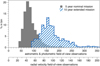 |
Fig. B.1. Counts of the simulated number of FoV observations of the 196 sky positions used in this study for a five- and ten-year Gaia mission (bin size: 10), see top panels of Fig. 6 for the corresponding sky-distribution. For radial velocity measurements, the number of FoV observations is reduced by a factor of 0.57 (4/7, see Sect. 2.2). |
Appendix C: Gaia astrometric FoV error model
With the Gaia mission and its calibration improvements still in progress, we adopt the same astrometric observation error model parameterisation described in Sect. 2.1 of Perryman et al. (2014). This error model provides the per-field-of-view astrometric centroiding error σfov, astro (μas) as a function of the host-star G-band magnitude:
![Mathematical equation: $$ \begin{aligned} z&= 10^{0.4(\mathrm{max}[G,12]-15)} \nonumber \\ \sigma _\eta&= (c_1\ z + c_2 \ z^2)^{0.5} \nonumber \\ \sigma _{\mathrm{fov,\,astro}}&= \left( \frac{ \sigma ^2_\eta }{9} + \sigma ^2_{\mathrm{att}} + \sigma ^2_{\mathrm{cal}} \right)^{0.5}\,{[\upmu \mathrm{as}]} \end{aligned} $$](/articles/aa/full_html/2022/05/aa36393-19/aa36393-19-eq40.gif) (C.1)
(C.1)
-
with
c1 = 53 000 and c2 = 310 in Perryman et al. (2014)
-
and
c1 = 49 000 and c2 = 1700 in this work (DR2 fit).
We note that for bright stars with G < 12, the observation times are reduced by CCD ‘gating’ to avoid signal saturation, causing a more or less constant measurement precision for these stars. In this error model, it is assumed to be strictly constant at a level of σfov = 34 μas per-FoV when adopting a value of 20 μas per-FoV for both  and
and  (Risquez et al. 2013; Lindegren et al. 2012), corresponding to a combined attitude and calibration noise level of 85 μas per CCD. The DR2 per-CCD astrometric centroiding precision shown in Fig. 9 of Lindegren et al. (2018) illustrates that the systematic noise level at that time was about 250 μas per CCD. Here, we make the realistic assumption that this noise level will reduce by a factor of three for the final astrometric data release due to improved calibration models, which is already (partially) corroborated by the improvements shown in Fig. A.1 of Lindegren et al. (2021).
The free parameters c1 and c2 of the Perryman et al. (2014) error model of Eq. C.1 were adjusted to fit the pre-launch prediction of the end-of-mission astrometric performance. We have revised this fit based on the estimates from DR2, as shown in Fig. C.1. The circles are DR2 median per-CCD formal uncertainties from Fig. 9 in Lindegren et al. (2018), converted to per-FoV estimates by dividing them by the square root of the nine per-FoV CCDs, and increased by 10% to match the actual robust scatter estimate observed, particularly for the fainter sources, in the Astrometric Global Iterative Solution (AGIS; Lindegren et al. 2012; O’Mullane et al. 2011; Lammers et al. 2010). The calibration precision is not expected to improve further for G > 13 where it is photon-limited.
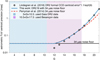 |
Fig. C.1. Adopted astrometric Gaia per-FoV precision model based on the expected Gaia precision derived from DR2 data, and compared with the Perryman et al. (2014) error model. |
The Perryman et al. (2014) and our DR2-derived error models agree within a few percent up to G ∼ 17, and start to deviate thereafter (8% at G = 17.5, 13% at G = 18, etc.), mainly due to the increased stray-light component in the real mission data. The planet detections predicted by Perryman et al. (2014) were brighter than G = 17 and hence the conclusions of these latter authors would be unchanged based on this latest model. Our results extend to G = 17.5, and hence this new error model will reduce the number of detections towards the faint end.
Appendix D: Gaia radial velocity FoV error model
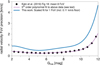 |
Fig. D.1. Adopted radial velocity Gaia per-FoV precision model valid for GRVS < 12, derived from Gaia DR2 radial velocity data. |
To compute the detectability of BD companions using the Gaia RVS derived radial velocity measurements (Sect. 2.2) we need an end-of-mission estimate of the per-FoV precision of the radial velocity measurements. Due to changes from the pre-launch conditions (e.g. the stray-light issue discussed by the Gaia Collaboration 2016b) we estimated the expected end-of-mission performance from the currently available data, i.e. Fig. 18 of Katz et al. (2019). We take the data points for the interval of [7,11] transits which have a mean at N = 8, and using their Eq. 1 we fit a fifth-degree polynomial model P(GRVS) to the ‘formal’ per-FoV transit uncertainty σVR:
![Mathematical equation: $$ \begin{aligned} \epsilon _{\mathrm{V}_{\rm R}} = \left[ \left( \sqrt{ \frac{\pi }{2\ N}} P(G_{\mathrm{RVS}}) + 0.11^2 \right) \right] \ \ \mathrm{with} \ \ P(G_{\mathrm{RVS}}) \simeq \sigma _{\mathrm{V}_{\rm R}} \ , \end{aligned} $$](/articles/aa/full_html/2022/05/aa36393-19/aa36393-19-eq43.gif) (D.1)
(D.1)
with the polynomial model
 (D.2)
(D.2)
For the adopted per-FoV precision we include a 0.11 km s−1 noise floor, which is the current best estimate for the end-of mission precision (David Katz, private communication), resulting in
![Mathematical equation: $$ \begin{aligned} \sigma _{\mathrm{fov,\,RV}} = \sqrt{ P^2(G_{\mathrm{RVS}}) + 0.11^2 } \ \ [\mathrm{km\,s}^{-1}] \ . \end{aligned} $$](/articles/aa/full_html/2022/05/aa36393-19/aa36393-19-eq45.gif) (D.3)
(D.3)
Appendix E: Gaia photometric FoV error model
To compute the detectability of photometric BDs transits (Sect. 2.3) we require an end-of mission estimate of the per-FoV precision of the G-band photometry. As for the radial velocity precision, we have replaced the pre-launch estimates with those from currently available data. In Fig E.1 we estimate the per-FoV G-band photometric precision (blue solid lines) from the published uncertainties on the mean, for both DR28 (black line) and EDR39 (scatter data). From this we see that above G > 16.5 the improvement in EDR3 is relatively small. From this observation, and the fact that it extends down to about G = 13.5 along a rather straight exponential line, we assume that the EDR3 mode line has reached the photon-limited precision and will no further improve in future releases. For the bright range, the gating complicates the calibrations, and it is clear that this has substantially improved in EDR3, and should continue to improve in the coming releases. Therefore, we adopted a simple noise floor of σFoV, G = 10−3 mag10, which effectively extends up to G ≃ 13.5. For G > 13.5, we fit a second-order polynomial to the mode of the EDR3 data, resulting in our adopted model, illustrated by the blue line:
![Mathematical equation: $$ \begin{aligned} \sigma _{\rm fov,G}&= 10^{\mathrm{max}\left[-3, -3.56 \ -0.0857\, x \ + \ 0.00938\, x^2 \right]} \ \ \mathrm{[mag]} \\ \mathrm{with } x&= G-0.15 \nonumber \ . \end{aligned} $$](/articles/aa/full_html/2022/05/aa36393-19/aa36393-19-eq46.gif) (E.1)
(E.1)
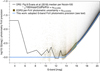 |
Fig. E.1. Adopted photometric Gaia G-band per-FoV precision model based on the approximate Gaia precision derived from EDR3 data. |
Appendix F: Cumulative density functions
To generate (MBD) from a uniformly distributed random number U ∼ U([0, 1]) we use the inverse cumulative density function. This is the inverse CDF of Eq. 8:
 (F.1)
(F.1)
where the coefficients correspond to those presented in Eq. 8. Using the same technique, the random sampling of the period and eccentricity distribution were performed, using the inverse functions of the CDF formulae given in Figs. 2 and 3.
Appendix G: Besançon model data for G > 10.5
To simulate the vast majority of the host star distribution, we used the latest 201611 Besançon model, which has various improvements over the model of 2013, including a variable star formation rate over the thin disc life time (Czekaj et al. 2014). The extinction distribution was set to the suggested Marshall et al. (2006) model for 100° < l < 100° and −10° < b < 10°, and diffuse extinction for higher latitudes and longitudes.
Simulations were generated in bins adjusted for three zones: (1) the ‘outer’ Galactic northern and southern hemispheres spanning 0° ≤l < 360° in steps of 36°, and 28° < |b|≤90° in steps of 6.2°; (2) the Galactic ‘centre’ region spanning −60° ≤l ≤ 60° in steps of 10°, and −28° ≤b ≤ 28° in steps of 3.5°; and (3) the Galactic ‘disc’ region spanning 60° < |l|≤180° in steps of 20°, and −28° ≤b ≤ 28° in steps of 3.5°.
The model includes the apparent Gaia G-band magnitude. Although the simulated G passband uses the pre-launch transmission curves described in Jordi et al. (2006, 2010), any differences with the in-flight passband will be negligible for the outcome of this study. The simulations were limited to spectral types from F0 to K9, and luminosity class IV (subgiants) and V (main sequence). A limit of G < 17.5 was adopted based on the low detection rates beyond this magnitude (see Appendix A), and otherwise rather excessive simulation data volume.
The Besançon model output contains generated stars that are sampled uniformly in density for each of the sky-position bins. The total number of generated sources is: 130 327 900 of which 92 863 736 (71%) are main sequence stars, and 37 464 164 (29%) are subgiants. Fig. 5 shows the distribution of stars: on the sky, as a function of magnitude, stellar type, and as a function of effective temperature versus mass and bolometric magnitude. The bottom panel has some visual guides at Teff = 7220 K and 3940 K, and Mbol = 2.50 and 7.59, corresponding to the main sequence F0 and K9 stars12 (Pecaut & Mamajek 2013). The Besançon model we extracted did not contain any stars with G < 10.2 mag. For this paper we therefore use Gaia DR2 derived data for G < 10.5 (Appendix H) and use the Besançon data for G > 10.5.
We also require GRVS to select sources which are assumed to have radial velocity time-series (i.e. GRVS < 12). As our Besançon data use the pre-launch Gaia magnitude system (Jordi et al. 2010), we use those relations to compute GRVS from the G-band magnitudes and colours. A GRVS = 12 corresponds roughly to G = 12.65 for our FGK main sequence and subgiant sample. Applying the exact limit of GRVS < 12 on our Besançon data with G > 10.5 results in a sample of 1.7 million stars.
Appendix H: Gaia DR2 derived data for G < 10.5
Because the Besançon model data did not contain stars brighter than G < 10.2, we derived the stellar distribution for G < 10.5 from Gaia DR2 data. For the simulations in this study we need positions, apparent G-band magnitudes, distances, stellar host masses, radii, and GRVS magnitude estimates. The position (Lindegren et al. 2018), apparent magnitude (Riello et al. 2018; Evans et al. 2018), and estimate of the radius (Andrae et al. 2018) are available in DR2.
For about 95% of DR2 sources the parallax_over_error> 5 (i.e. relative error better than 20%) which means that a simple inverse of the parallax provides a meaningful distance, although it can still be biassed and have a large uncertainty. As we are mainly interested in the local stellar density, we used the Bayesian estimated distances with Galactic prior of Bailer-Jones et al. (2018) to derive a meaningful distance estimate for the whole sample13. Distances for our final sample typically deviate from the inverse parallax by less than 1% (and by a maximum of 8%).
To make a (initial) selection of main sequence and subgiants stars we use the main sequence selection of FGK stars in Gaia DR2 described in Sect. 3.1 of Hsu et al. (2019), with their suggested GBP − GRP range of [0.5, 1.7]. We made the following DR2 archive selection: lum_val < 3*1.75*power(10, 2.62 - 3.74*bp_rp + 0.962*bp_rp*bp_rp), where we added the factor 3 to confidently include the increase in luminosity from main sequence to subgiant phase (which is around 3 for solar-type stars, and more like 1.8 for F-type stars), resulting in a preliminary selection of 204 433 stars. In the Hsu et al. (2019) paper, the power of 10 was erroneously not mentioned (Danley Hsu, priv. comm.).
Mass estimates were not yet included in DR2. In comparison with the brightest part of the Besançon data, masses of the current observable sample can be reasonably well estimated from the absolute magnitude alone, with a dispersion of about 0.2 M⊙. We fit this relation with a quadratic function for the zero-age main sequence masses of the FGK stars listed in Pecaut & Mamajek (2013)12:  , which correctly follows the core of the distribution of both the main sequence and subgiants in Besançon mass versus G − 5log10(distance[pc])+5 (extinction correction does not have a large effect). Because the most massive stars in our sample (F0) should not exceed 1.6 M⊙, we select only stars with M < 1.6 M⊙. This modifies our initial selection based on the luminosity as a function of GBP − GRP such that the most luminous tip at the blue end gets clipped around a luminosity of 8.5 L⊙, which is similar to a F0V zero-age main sequence luminosity of 7.8 L⊙, and about 1.8 times less than 4.6 L⊙ for a F3V zero-age main sequence star (Pecaut & Mamajek 2013)12, illustrating that such a cut should roughly retain the relevant subgiants and not include too many giants. We estimate the absolute magnitude for the Gaia DR2 sources using phot_g_mean_mag - 5*log10(r_est [pc]) + 5. The extinction a_g_val is missing for about 25% of the sources in our selection and for those who have it, it causes peculiar (non-physical) structures in our HR-diagram, hence we omit any extinction correction. We then estimate the masses based on this derived absolute magnitude and apply the mass-cut of M < 1.6 M⊙ which reduces our Gaia DR2 sample to a final 174 122 stars with G < 10.5.
Additionally, we would like to roughly separate the main sequence stars from the subgiants, as in the Besançon data. The Besançon data shows that a cut of R⊙ > 1.7 should contain the vast majority of the subgiants, and below that the vast majority of the main sequence stars. This makes sense given that this it about the zero-age main sequence radius of our largest considered stars (F0V-F1V; Pecaut & Mamajek 2013)12. Even though this separation is not perfect, the distributions of the Besançon and Gaia DR2-selected data sets overlap rather well in the colour–magnitude diagram, and are consistent with their expected location in this diagram. In this way, we classify the selected 174 122 DR2 stars into 113 832 (65%) main sequence stars and 60 290 (35%) subgiants.
Finally, we need GRVS to select sources which are assumed to have radial velocity time-series (i.e. GRVS < 12). We adopted the approximate 0.65 mag mode offset derived from the Besançon data to convert DR2 photometry into GRVS for all DR2 stars irrespective of colour, i.e. GRVS, DR2 = GDR2 − 0.65. The standard deviation around this offset in the Besançon model was about 0.11 mag, hence we expect this fixed-value offset approximation to give meaningful approximations to the real GRVS. In conclusion, stars assumed to have radial velocity time-series (i.e., GRVS < 12) were selected in the DR2 data using the cut G < 12.65. We note that a more accurate GRVS conversion for DR2 data is provided in Eq. 2 and 3 of Gaia Collaboration (2018).
All Tables
Number of simulated BD detections from Gaia astrometry, radial velocity, and photometric transits.
Simulation results from bootstrapping with a BD sample from Raimbault (in prep.).
All Figures
|
Fig. 1. Adopted BD mass distribution in this study; see text for details. |
| In the text | |
|
Fig. 2. Period distribution of the BD sample from Ma & Ge (2014) and Díaz et al. (2012) which have masses of between 9 and 90 MJ orbiting solar-type stars. Top: cumulative distribution function for BDs. The ‘large P’ fits of Ma & Ge and Díaz are used to generate the BD period distributions and are referred to as Pdistr = Ma & Ge and Pdistr = Díaz, respectively. Bottom figure: log-binned histogram with the corresponding fit curves (bin size log10(1.98)). Our simulations are limited to the indicated (non-shaded) period range 1 d < P< 5 yr. The Raimbault (in prep.) data are used for an additional bootstrap sample estimate (Sect. 5.2). |
| In the text | |
|
Fig. 3. Eccentricity distribution of the BD sample from Ma & Ge (2014) and Díaz et al. (2012). Top: cumulative distribution function for BDs. The ‘Ma & Ge’ fit is used for the simulations in this paper. Bottom figure: binned histogram with the corresponding fit curve (bin size 0.05). Raimbault (in prep.) data are used for an additional bootstrap sample estimate (Sect. 5.2). |
| In the text | |
|
Fig. 4. Period–eccentricity distribution of the BD samples from the three sources considered in this study: (1) Ma & Ge (2014) split into low-mass and high-mass samples, (2) Díaz et al. (2012), and (3) that from Raimbault (in prep.) but only for BDs with companions in the 10 − 80 MJ sin i range. In our simulations, a circularisation limit of 10 d is adopted, resulting in the eccentricity limit indicated by the black line. We limit (most of) our derived models to the interval between the shaded areas, namely 1 d < P< 5 yr. |
| In the text | |
|
Fig. 5. Distribution of the 130 million simulated FGK main sequence (MS) and subgiants (SG) host stars with G < 17.5. Top: logarithmic Galactic sky density (Besançon data only). Second: histogram of G-band counts (bin size: 0.5 mag). Third: Histogram of colour (bin size: 0.1) and type (bin size: 0.2). Bottom: colour–absolute magnitude diagram (Besançon data only). |
| In the text | |
|
Fig. 6. Distributions of the astrometric and radial velocity solid detections (Δχ2 > 50) resulting from the Pdistr = ‘Ma & Ge’ simulation. Top: number of FoV transits for comparison with lower panels. Second: astrometric detections. Third: radial velocity detections. Bottom: histogram of counts as a function of colour (bin size: 0.05), separated by evolutionary stage. |
| In the text | |
|
Fig. 7. Histograms of the astrometric and radial velocity solid detections (Δχ2 > 50) resulting from the Pdistr = ‘Ma&Ge’ simulation. Top panel: host star magnitude. Second panel: period. Third panel: distance. Fourth panel: BD mass. Bottom panel: semi-major axis |
| In the text | |
|
Fig. 8. Distributions of the BDs resulting from the five-year (left) and ten-year (right) Gaia simulations using Pdistr = Ma & Ge for the three adopted astrometric detection thresholds: Δχ2 > 30 (41 000, 64 000), Δχ2 > 50 (28 000, 45 000), and Δχ2 > 100 (17 000, 28 000). (The point-cloud data are from 1% simulations (Sect. 3.3), hence scale by 0.6 to get the BD rates of Table 1.) |
| In the text | |
|
Fig. 9. Same as Fig. 8 but now for the three adopted Gaia radial velocity detection thresholds (i.e. limited to stars with GRVS < 12): Δχ2 > 30 (1700, 2700), Δχ2 > 50 (1100, 1900), and Δχ2 > 100 (570, 1100). (The point-cloud data are from 1% simulations (Sect. 3.3), hence scale by 0.6 to get the BD rates of Table 1.) |
| In the text | |
|
Fig. 10. Intersection of Figs. 8 and 9, i.e. where the same detection threshold is passed for both Gaia astrometry and radial velocity (hence limited to stars with GRVS < 12): Δχ2 > 30 (810, 1600), Δχ2 > 50 (410, 950), and Δχ2 > 100 (140, 400). (The point-cloud data are from 1% simulations (Sect. 3.3), hence scale by 0.6 to get the BD rates of Table 1.) |
| In the text | |
|
Fig. 11. Transit statistics from the Pdistr = Ma & Ge simulation for a five-year and ten-year mission of 1.5 million randomly oriented BDs. These BD number counts are scaled by 0.6 to represent a 0.6% BD occurrence rate in Table 1; see Sect. 3.3. Detailed period-binned statistics of the ‘ALL’ part are shown in Table 2. |
| In the text | |
|
Fig. A.1. Astrometric eccentricity dependence of distance and magnitude detection limits for Δχ2 = 100 for a G2V star and a 10 MJ BD with P = 4 yr. The black point at e = 0 corresponds to the black point in the middle panel of Fig. A.2. Sky-detection fractions of 50 percentile (thick line) and 10–90 percentile (shaded region) illustrate that the detection threshold for such a (randomly oriented) system varies by ±25%, depending on sky position. |
| In the text | |
|
Fig. A.2. Illustration of the Gaia astrometric and radial velocity detection limits for the adopted BD mass range 10– 80 MJ around a F0V/G2V/K6V main sequence star (top/middle/bottom respectively) for different Δχ2 detection thresholds (see Sect. 2.1) resulting from a simulated five-year nominal mission (left) and ten-year extended mission (right). For each Δχ2 detection threshold, the lines show for a given period (bottom axis) and semi-major axis (top axis), the zero-extinction limits in distance (left axis) and apparent G-band magnitude (right-axis) for which 50% of the simulated sky positions are no longer detectable. The ascending thick lines are the astrometric limits, while the descending thin lines are the radial velocity limits. We note that the latter are truncated due to the GRVS = 12 limit (see text for details). For the dot in the middle panel, the astrometric eccentricity dependence and sky-position variation is expanded in Fig. A.1; see Sect. A for more details. For comparison, in grey we include the astrometric detection thresholds for a 1 MJ planet (it is not detectable using Gaia radial velocity). |
| In the text | |
|
Fig. B.1. Counts of the simulated number of FoV observations of the 196 sky positions used in this study for a five- and ten-year Gaia mission (bin size: 10), see top panels of Fig. 6 for the corresponding sky-distribution. For radial velocity measurements, the number of FoV observations is reduced by a factor of 0.57 (4/7, see Sect. 2.2). |
| In the text | |
|
Fig. C.1. Adopted astrometric Gaia per-FoV precision model based on the expected Gaia precision derived from DR2 data, and compared with the Perryman et al. (2014) error model. |
| In the text | |
|
Fig. D.1. Adopted radial velocity Gaia per-FoV precision model valid for GRVS < 12, derived from Gaia DR2 radial velocity data. |
| In the text | |
|
Fig. E.1. Adopted photometric Gaia G-band per-FoV precision model based on the approximate Gaia precision derived from EDR3 data. |
| In the text | |
Current usage metrics show cumulative count of Article Views (full-text article views including HTML views, PDF and ePub downloads, according to the available data) and Abstracts Views on Vision4Press platform.
Data correspond to usage on the plateform after 2015. The current usage metrics is available 48-96 hours after online publication and is updated daily on week days.
Initial download of the metrics may take a while.