| Issue |
A&A
Volume 660, April 2022
|
|
|---|---|---|
| Article Number | A119 | |
| Number of page(s) | 16 | |
| Section | Extragalactic astronomy | |
| DOI | https://doi.org/10.1051/0004-6361/202142253 | |
| Published online | 22 April 2022 | |
Discovery of late-time X-ray flare and anomalous emission line enhancement after the nuclear optical outburst in a narrow-line Seyfert 1 Galaxy
1
Department of Physics, Anhui Normal University, Wuhu, Anhui 241002, PR China
e-mail: xwshu@mail.ahnu.edu.cn
2
CAS Key Laboratory for Researches in Galaxies and Cosmology, Department of Astronomy, University of Science and Technology of China, Hefei, Anhui 230026, PR China
e-mail: shengzf@ustc.edu.cn, jnac@ustc.edu.cn
3
Department of Astronomy, Guangzhou University, Guangzhou 510006, PR China
4
Yunnan Observatories, Chinese Academy of Sciences, Kunming 650011, PR China
Received:
18
September
2021
Accepted:
13
January
2022
CSS J102913+404220 is an atypical narrow-line Seyfert 1 galaxy with an energetic optical outburst occurring co-spatially with its nucleus. We present a detailed analysis of multi-wavelength photometric and spectroscopic observations of this object covering a period of a decade since outburst. We detect mid-infrared (MIR) flares delayed by about two months relative to the optical outburst and with an extremely high peak luminosity of L4.6 μm > 1044 erg s−1. The MIR peak luminosity is at least an order of magnitude higher than any known supernovae explosions, suggesting the optical outburst might be due to a stellar tidal disruption event (TDE). We find late-time X-ray brightening by a factor of ≳30 with respect to what is observed about 100 days after the optical outburst peak, followed by a flux fading by a factor of ∼4 within two weeks, making it one of the active galactic nuclei (AGNs) with extreme variability. Despite the dramatic X-ray variability, there are no coincident strong flux variations in optical, UV, and MIR bands. This unusual variability behavior has been seen in other highly accreting AGNs and could be attributed to absorption variability. In this scenario, the decrease in the covering factor of the absorber with accretion rate could cause the X-ray brightening, possibly induced by the TDE. Most strikingly, while the UV/optical continuum remains almost unchanged with time, an evident enhancement in the flux of the Hα broad emission line is observed about a decade after the nuclear optical outburst, which is an anomalous behavior never seen in any other AGN. Such an Hα anomaly could be explained by the replenishment of gas clouds and excitation within the broad line region (BLR) that perhaps originates from its interaction with outflowing stellar debris. Our results highlight the importance of the late-time evolution of a TDE, which can affect the accreting properties of the AGN, as suggested by recent simulations.
Key words: galaxies: active / galaxies: nuclei / X-rays: individuals: CSS J102913+404220 / galaxies: Seyfert / accretion / accretion disks / X-rays: bursts
© ESO 2022
1. Introduction
It is believed that active galactic nuclei (AGNs) are powered by supermassive black holes (SMBHs, MBH ∼ 106 − 109 M⊙) accreting surrounding material. The optical and UV photons emitted by AGNs are thought to originate from the accretion disk, and a fraction of disk emission is transported into the hot corona, presumably in the immediate vicinity of the SMBH, generating powerful X-rays at higher energies. While rapid X-ray variability over a timescale from minutes to hours is ubiquitous in AGNs (Ulrich et al. 1997; González-Martín & Vaughan 2012), large-amplitude variations on longer timescales of years are not common, as the long-term variability amplitude is typically in the range ∼50−200% (Saxton et al. 2011; Yang et al. 2016; Middei et al. 2017; Boller et al. 2022). In addition, exotic AGN X-ray variability characterized by quasi-periodic modulations (Gierliński et al. 2008; Song et al. 2020) or even repeating short-lived X-ray eruptions (Sun et al. 2013; Miniutti et al. 2019) are also found, providing a unique probe to the accretion physics and X-ray radiation mechanisms.
Extreme X-ray variability of orders of magnitude on timescales of years has been found in several types of AGNs (e.g., Grupe et al. 2012a), some of which is also accompanied by X-ray spectral changes, i.e., from Compton-thin to Compton-thick or vice versa. This latter case can be naturally explained in terms of variations of absorption column density along the line of sight (e.g., Risaliti et al. 2005; Miniutti et al. 2014). Alternatively, the dramatic X-ray flux and spectral variations can be ascribed to the “switch off and on” of the gas accretion onto SMBHs (Guainazzi et al. 1998; Gilli et al. 2000).
However, such a scenario is difficult to reconcile with the observations of X-ray weak state in several highly accreting narrow-line Seyfert 1 galaxies (NSy1s) and quasars, where the UV flux remains almost constant despite the huge X-ray drop (Gallo et al. 2011; Miniutti et al. 2012; Grupe et al. 2019). As sources with high Eddington ratios such as NSy1s are expected to have a geometrically thick accretion disk in the innermost region, the disk self-shielding can explain the extreme X-ray variability while UV/optical continuum at larger radii is not affected, similar to the explanation proposed for the X-ray behavior of weak-line quasars (Luo et al. 2015; Ni et al. 2018). Another scenario that has been invoked to account for the X-ray weakness is that the direct nuclear emission is suppressed by the light-bending effect near the SMBH (Miniutti et al. 2003; Miniutti & Fabian 2004).
While extreme X-ray variations appear to be rare among standard AGNs, they are more commonly seen in stellar tidal disruption events (TDEs; see Komossa 2015 for a review). Such events occur when a star passes sufficiently close to a SMBH and the star is torn apart when the tidal force of the SMBH exceeds its self-gravity. While roughly half of the stellar material will be ejected, the other half will remain bound and eventually be accreted, producing a luminous flare of electromagnetic radiation (Rees 1988). For a BH mass with MBH ∼ 106 M⊙, the peaking luminosity can reach ∼1044 erg s−1 and then declines by up to factors of > 100 to the quiescent flux level of the host galaxy. X-ray observations have revealed a population of TDE candidates with such large-amplitude X-ray variability (e.g., Komossa 2015; Lin et al. 2017; Saxton et al. 2019). We note that similar extreme optical outbursts in the centers of galaxies were recently detected, but very few of them are associated with strong X-ray emission, the nature of which is still under debate (Kankare et al. 2017). In addition, theoretical works have suggested that TDEs can occur in AGNs and the event rate may be even higher than in inactive galaxies (Karas & Šubr 2007). Indeed, an increasing number of TDE candidates have been found in galaxies with pre-existing AGN activity (e.g., van Velzen et al. 2016; Blanchard et al. 2017; Shu et al. 2018; Liu et al. 2020). However, in this case, identifying whether nuclear outburst is due to a TDE or a particular episode of AGN variability is not trivial (Saxton et al. 2015; Auchettl et al. 2018; Trakhtenbrot et al. 2019; Hinkle et al. 2021). On the other hand, in the presence of a TDE, the innermost regions of the accretion flow can be affected by the evolution of stellar debris, leading to unique and remarkable AGN X-ray variabilities (Blanchard et al. 2017; Chan et al. 2019; Ricci et al. 2020, 2021).
CSSJ102912.58+404219.7 (hereafter CSS1029) is a NSy1-like galaxy at z = 0.147 that was discovered by the Catalina Real-time Transient Survey (CRTS; Drake et al. 2009) as an extraordinary optical transient in the galaxy nucleus (Drake et al. 2011; D11 hereafter). Its extremely high peak luminosity of MV = −22.7, distinctive features of hydrogen Balmer emission lines, and the slow rise and fall of its light curve over a period of months led D11 to classify the transient as a ultra-luminous Type IIn supernova. However, based on its similar spectral properties to those of PS16dtm, another luminous transient occurring at the nucleus of a NSy1, Blanchard et al. (2017) suggested that CSS1029 is more like a nonstandard TDE (see also Kankare et al. 2017). The recent argument that the superluminous supernova (SLSN) ASASSN-15h is more consistent with a TDE (Leloudas et al. 2016) suggests that the bright optical outburst in CSS1029 may not necessarily be due to a SLSN. Here, we present new optical spectroscopy as well as archival multi-wavelength observations of CSS1029, and confirm the source as one of most luminous nuclear transients in terms of mid-infrared (MIR) luminosity, thus possibly ruling out its association with a Type IIn SLSN. In particular, we find a bright X-ray flare about five years post-optical-outburst, while no obvious coordinated photometric variability at other bands is found. Most strikingly, our spectroscopy follow-up observations about a decade later reveal a significant flux enhancement in the Hα emission line, while the continuum emission remains almost constant. This kind of Hα variability is anomalous and rare among either TDEs or NSy1s. In Sect. 2, we describe the observations and data reductions. In Sect. 3, we present a detailed analysis and results. Possible explanations for the late-time X-ray brightening and Hα anomaly are given in Sect. 4.
2. Observations and data
CSS1029 was first discovered as a bright optical transient on Feb 17 2010 (D11). Prompt Swift observations of the source were performed four times in 2010. There are also seven follow-up Swift observations performed in 2015, and two observations in 2020. Details of the observation information are listed in Table 1. Some results from the Swift 2010 observations were presented in D11, while the data after 2015 have not yet been fully reported. For the Swift/XRT (X-ray Telescope) data, all of them were obtained in Photon Counting (PC) mode. After reducing the data following standard procedures in xrtpipline, we used Heasoft (v6.19) to extract the spectrum with the task xselect. The source spectrum was extracted in a circular region with a 40″ radius, and we used another source-free circular region with a radius of 100″ for background. We generated ancillary response function files (ARFs) using xrtmkarf, and the response matrix files (RMFs) were downloaded with the latest calibration files.
X-ray count rates, fluxes, and optical magnitudes for CSS1029 observed by Swift.
For Swift UVOT (the Ultra-violet Optical Telescope) data, all four observations in 2010 have data in six filters (UVW2, UVM2, UVW1, U, B, V). By giving the source coordinate from optical position, we obtained magnitudes in the six bands for each observation using the task uvotsource. We performed flux extraction for source and background using a circular region with 5″ radius and a source-free circular region with 50″ radius, respectively. In observations performed in 2015, only three UV band filters were used, and the source and background flux were extracted using the same manner as for the 2010 data. All the UVOT magnitudes are referred to using the AB magnitude system, and are listed in Table 1. We note that the UVOT measurements are consistent with the results of D11, where only the data taken on 2010 are presented.
We performed follow-up long-slit optical spectroscopy observations of CSS1029, aiming to examine any spectral evolution at later times. The observations were taken twice with the Double Beam Spectrograph (DBSP) on the 200-inch Hale telescope at Palomar Observatory (P200) in February 2018 and February 2020. The latter is quasi-simultaneous with the recent X-ray observations. We used the D55 dichroic which splits the incoming photons into the 600/4000 (lines/mm) grating for the blue side, and 316/7500 grating for the red side.
The grating angles were adjusted so that a nearly continuous wavelength coverage from 3300 to 10 000 Å is obtained, with a spectral resolution of R = λ/Δλ ∼ 1080 at λ ∼ 6600 Å. The data were reduced following the standard procedures. The default slit width for the DBSP observations is 1.5″. Although the observations have different seeing conditions, namely 3.3″ for February 2018 and 1.5″ for February 2020, we used the same aperture size of ∼1.5″ to extract the spectrum, with the aim being to mitigate potential effects on flux measurements of continuum and emission lines with different apertures. The spectrum was then flux calibrated using standard star observations from the same night. In addition, we also observed the source with the YFOSC (Yunnan Faint Object Spectrograph and Camera) mounted on the Lijiang 2.4m telescope at the Yunnan Observatory in April 2020, January 2021, and May 2021, respectively. For the former two YFOSC observations, we used the spectral settings of G8 grating plus a slit width of 2.5″, while for the latter we used a slit width of 1.8″. The observations were performed under a typical seeing of ∼2″. The G8 grating covers a wavelength range from 5100 to 9600 Å, with a spectral resolution of R ∼ 380 at λ ∼ 6600 Å for the 2.5″ slit, and R ∼ 810 for the 1.8″ slit, respectively.
The YFOSC data were reduced using standard techniques in IRAF and the same aperture of 1.5″ was used to extract the spectrum. Details of the spectroscopic observations are listed in Table 3, including date, seeing, exposure, spectral resolution, and spectral extraction aperture at each epoch.
3. Analysis and results
3.1. X-ray variability
As mentioned above, D11 reported the X-ray detection from observations in 2010, but did not give the details of X-ray properties. We show that the source is clearly not detected in the last of the four observations in 2010, indicating a significant flux decay.
Here we present a detailed and uniform analysis of all archival X-ray observations, especially for those that are not given in D11, aiming to further investigate the X-ray flux and spectral evolution on longer timescales.
Figure 1 (left) plots the evolution of X-ray luminosity in the 0.3–2 keV for the observations taken in 2010, and a 3σ upper limit is shown for the nondetection1. The X-ray flux was converted from count rate using the best-fitting power-law model to the stacked spectrum (Sect. 3.2). It is evident that the source brightness declined by a factor of ≳3 over a period of ∼50 days, from 5.6 ± 1.8 × 1042 erg s−1 to the upper limit of 9 × 1041 erg s−1. Such an evolution of X-ray brightness is not uncommon if due to a TDE (Blanchard et al. 2017), but no conclusive evidence can be drawn as X-ray variability by even larger factors is often observed in NSy1s. To gain further insight into the nature of X-ray emission, we present the evolution of host-subtracted optical luminosity at the V-band during the period of outburst (gray dots). We estimate the host galaxy flux from the plateau of the light curve before the optical outburst, which is 17.51 ± 0.1 mag and is consistent with that estimated by D11. We note that we used the post-DR2 data from the CRTS survey to construct the host-subtracted light curve (Graham et al. 2017), and so it is slightly better sampled than that presented in D11 where only data up to ∼300 days after outburst are shown. While the luminosity evolution can be well described by an exponential law L = L0e−(t − t0)/τ, the fit with the popular t−5/3 decay law is worse, especially for the data taken after ∼150 days post-peak.
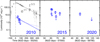 |
Fig. 1. X-ray light curves observed at different epochs. Left panel: the evolution of the host-subtracted optical luminosity at the V-band is also shown (gray points, in units of 1042erg s−1). The solid line shows the best exponential fit, while the dotted line is the fit with the canonical t−5/3 decay law. The two best-fit lines are scaled down by a factor of 100 to match the X-ray light curve. |
Although the X-ray luminosity appears to follow a similar evolution (blue curves), it is nearly two orders of magnitude lower than the optical luminosity at the same epochs. We discuss possible reasons for the relative faintness of the X-ray emission in Sect. 4.2.
Although the source becomes invisible in the last observation performed in 2010, Swift detected it again in 2015 in X-rays (Fig. 1, middle). The highest luminosity recorded is 5.5 ± 1.3 × 1043 erg s−1, corresponding to a rebrightening by a factor of > 30 relative to the previous nondetection. In addition, the source declines in flux quickly by a factor of ∼4–10 over two weeks.
A previous study of CSS1029 whereby individual observations were stacked claimed the detection of X-ray emission in 2015 to be of the same order of magnitude as the first observation in 2010 (Auchettl et al. 2017). However, this is not true when considering the flux decay and particularly the difference between the lowest state in 2010 and highest state in 2015, which are not considered in past analyses. While the source is detected in the first observation performed in January 2020 with ∼6 ± 2 net counts, it becomes invisible again in the second observation about a month later (Fig. 1, right). Although we lack enough X-ray observations to monitor the luminosity evolution since 2015, the above analysis suggests that CSS1029 shows a long-term X-ray variability by factors of ∼10 on timescales as short as a few tens of days, which is consistent with what is seen in NSy1s.
3.2. X-ray spectral analysis
Because of short exposures, the spectral signal-to-noise ratios (S/Ns) for most of the individual Swift observations are not sufficient to perform meaningful fittings. Therefore, in order to obtain a spectrum with a better S/N, we combined the spectra from individual observations using the FTOOLS task addascaspec. We added spectral files separately from the three Swift observations taken in 2010 (Swift 2010), and five observations in 2015 (Swift 2015). Nondetections are excluded in the spectral stacking (Table 1). We obtained 17 ± 5 and 82 ± 9 background-subtracted counts in the 0.3–5 keV range for the Swift 2010 and 2015, respectively. As only 6 ± 3 net counts are detected in the first Swift observation performed in 2020, we do not consider the 2020 data in the following spectral analysis. The Swift 2010 spectrum appears soft, with most of the counts falling below 1.5 keV (∼80%). For the Swift 2015 observations, we detected 11 net counts at energies above 1.5 keV, indicating the presence of harder X-ray emission (Fig. 2). In the following spectral analysis, we grouped the data to have at least two counts in each bin to ensure the use of the C-statistic for the spectral fittings.
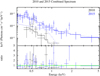 |
Fig. 2. X-ray spectrum by stacking three observations in 2010 (black) and five observations in 2015 (blue). The dotted line shows the best-fitted model consisting of a power law and a blackbody component. We note that the spectral fittings were performed jointly to the 2010 and 2015 data based on this model. The corresponding data-to-model ratios are shown in the bottom panel. |
The Galactic column density was considered and fixed at  cm−2. All statistical errors given hereafter correspond to ΔC = 2.706 for one interesting parameter, unless stated otherwise.
As a first step, we performed the spectral fittings to the combined Swift 2015 spectrum –which has the best spectral quality– using a simple absorbed power-law model. The fitting result is acceptable, with a power-law index  and C/d.o.f. = 36.4/40. The intrinsic absorption is not required, with an upper limit on the column density of NH < 1 × 1021 cm−2. Although loosely constrained, the power-law component is relatively steep among AGNs (Grupe et al. 2010). We therefore attempted to fit the spectrum with a blackbody (zbbody in XSPEC), but found an excess of emission at energies above ∼1.5 keV. The addition of a power law to the model improves the fit significantly (C-value is decreased by 24.9 for two extra parameters). In this case, we obtain a blackbody temperature of kTBB = 101 ± 28 eV, and the power-law component becomes flatter with
  , which are consistent with the typical values observed in NSy1s. The spectral fitting results are summarized in Table 2.
Spectral fitting results for the Swift 2010 and 2015 data.
A similar spectral analysis was also performed for the Swift 2010 data, which can be described by a simple absorbed power-law model with photon index  . The photon index is comparable to that observed in TDEs which can be ascribed to the thermal disk emission at soft X-ray bands (Komossa 2015).
We found a single blackbody model providing an equally good fit to the Swift 2010 data, without the requirement for an additional power-law component. As the spectral quality is poor for the 2010 data, we cannot tell whether the source is intrinsically weak at hard X-rays or such a component has simply eluded detection due to insufficient exposure. Given that the 0.3–1 keV spectral shape is consistent between the 2010 and 2015 observations, we then considered a joint fit to the two data sets in the 0.3–5 keV range. We used the best-fitting model for the 2015 spectrum, which comprises a thermal blackbody emission plus a power law component, modified by the Galactic absorption. All the parameters are fixed to be the same except for flux normalizations. We obtained an acceptable joint fit (C/d.o.f. = 43.2/48) with kT ∼ 101 eV and Γ ∼ 2.04. Based on this model, we found an 0.3–2 keV flux of 7.02 × 10⁻¹⁴erg cm−2 s−1 and 5.42 × 10⁻¹³erg cm−2 s−1, and 2–10 keV flux of 1.98 × 10⁻¹⁴erg cm−2 s−1 and 1.53 × 10⁻¹³erg cm−2 s−1 for the 2010 and 2015 data, respectively. We note that the hard X-rays are clearly not detected for the 2010 observations, and therefore the above 2–10 keV flux from the model extrapolation may only serve as an upper limit.
3.3. Ultraviolet emission and optical-to-X-ray spectral energy distribution
As we show above, the X-ray emission appears relatively faint during the period of optical outburst in CSS1029. In order to gain insights into the X-ray properties, we now turn to the analysis of the UV emission and its flux ratio to X-rays.
All the Swift observations provide simultaneous UV photometric data through UVOT in the filter UVW2 (λc = 1928 Å), UVM2 (λc = 2246 Å) and UVW1 (λc = 2600 Å), respectively. For the observations performed in 2010 and 2020, the simultaneous optical data are also available (Table 1). It is interesting to note that while the X-ray flux increases by a factor of up to > 30 between 2010 and 2015 observations, the UV variations on the hand have much smaller amplitudes. For example, the maximum UV variation for the UVW2 is ∼1.54 mag, corresponding to only a factor of ∼4 drop in the monochromatic flux between the two epochs. The UV variations are also not strongly correlated with the X-ray ones within each epoch.
The availability of simultaneous UV and X-ray data allows us to reliably derive the UV-to-X-ray slope for each observation. The UV-to-X-ray slope is often defined by monochromatic flux ratio between 2 keV and 2500 Å in the rest frame, parameterized with αox = 0.384log(f2 keV/f2500 Å).
To calculate the 2500 Å flux, we used the observed flux at the bluest UV band (∼1928 Å, UVW2), which is expected to be less affected by host contamination. The UVW2 flux was then extrapolated to the 2500 Å by assuming a typical UV spectral index of α = 0.65 (Sν ∝ ν−α, Grupe et al. 2010). We note that adopting a different slope of α between 1 and 0 in the extrapolation would result in a change of ≲50% in the 2500 Å flux and therefore of ≲20% in the αox. The X-ray flux density at 2 keV was estimated by the best-fitting model that was used to perform the joint fit to the 2010 and 2015 data, and corrected for the Galactic absorption (Sect. 3.2). The model consists of a power law with Γ = 2.04 and a blackbody component with kT = 101 eV.
In order to avoid introducing model-dependent biases, we adopted the same model to estimate the 2 keV flux for the Swift 2020 data. As no X-rays above 1.5 keV are detected for the 2010 and 2020 observations, we considered all the αox as upper limits for these epochs. Our measurements imply that CSS1029 has a much steeper UV-to-X-ray spectral slope (αox ≲ −2) in 2010 than that in 2015 (αox ≃ −1.5).
It is well known that the αox are correlated with the 2500 Å luminosity for AGNs, which are increasingly X-ray weak for higher UV luminosities (e.g., Steffen et al. 2006). Such a relation for the X-ray-selected AGNs is shown by the solid line (Grupe et al. 2010) in Fig. 3 (left), and the dotted line represents the approximately 1σ scatter of the distribution. The NSy1s from the sample are shown in gray filled circles, while the broad-line Sy1s are shown in triangles.
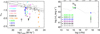 |
Fig. 3. Left: UV-to-X-ray spectral index αox versus 2500 Å luminosity for CSS1029 (black, green and blue symbols). The solid line represents the fit to the X-ray-selected AGNs from Grupe et al. (2010). The NSy1s are shown as gray dots, while the broad-line Sy1s are shown as gray triangles. For comparison, we also plot the αox for four typical NSy1s with extreme X-ray variations. The αox were calculated in the same manner as CSS1029. For clarity, only the two data points representing observations between the high and low state are shown. The open star represents the data for the thermal TDE ASASSN-14li in the flare state (van Velzen et al. 2016). Right: optical to X-ray SED of CSS1029. For clarity, only the data for the highest and lowest state within each epoch are shown. The median SED from radio-quiet quasars (Elvis et al. 1994) is also shown for comparison (dotted line), for which the luminosity is scaled to that of UVW2 obtained in the high state in 2015. |
It can be seen that the αox ≃ −1.35 at the highest state (rebrightening stage in 2015) is relatively typical for CSS1029 as a normal NSy1. However, the source became increasingly X-ray weak in the subsequent observations, down to an X-ray level comparable to that obtained with the most recent observations in 2020, falling significantly below the extrapolation of the αox − L2500 Å relation. The average Δαox = αox − αox, exp = −0.191 and < −0.379 for the 2015 and 2020 data2 is consistent with the source being X-ray weaker than αox, exp at a 2.38σ and 4.74σ level, respectively. In comparison with the 2015 and 2020 data, CSS1029 is even more (hard) X-ray weak in 2010 according to the Δαox. Such an extreme X-ray weakness is unusual among AGNs, when compared with the NSy1s in an extreme X-ray faint state, such as Mrk 335 (Grupe et al. 2012b), 1H0707 (Fabian et al. 2012), IRAS F13324-3809 (Buisson et al. 2018), and RX J2317.8-4422 (Grupe et al. 2019). This is similar to the X-ray-weak quasar phenomenon, as exhibited by PHL 1092 from XMM-Newton monitoring observations (Miniutti et al. 2012), suggesting CSS1029 might be one of the AGNs with the most extreme αox variability ever found. Alternatively, such an X-ray weakness might be expected if the X-ray emission was dominated by a soft blackbody component as originated from the transient disk accretion in the process of TDE. Indeed, ultrasoft X-ray spectra have been found to be common in TDEs (Komossa 2015; Auchettl et al. 2017). We also plot the αox (open star in Fig. 3 (left)) for the best-studied thermal TDE ASASSN-14li in the flare state (e.g., van Velzen et al. 2016), and find it is comparable to the 2010 data for CSS1029, suggesting a possible connection between the two.
A further perspective on the unusual X-ray properties of CSS1029 comes from the detailed comparison of optical-to-X-ray spectral energy distribution (SED) between different epochs, as shown in Fig. 3 (right). For clarity, we show only the data from the high and low state for the three epochs. The recent Swift observations in 2020 revealed a similar flux to the one in the last observation of 2015, followed by a drop by a factor of ≳3 within ∼50 days, indicating a possibly new X-ray variability. For comparison, the median SED of radio-quiet quasars, scaled to the UVW2 flux in the 2015 high state, is also shown (dotted line). The UV-to-X-ray SED of CSS1029 in the 2015 high state is consistent with those of typical quasars, while it is X-ray weak by an order of magnitude in the low state; the same is seen in the 2020 data.
We note that the optical-to-X-ray SEDs for observations in 2010 might be different from the median SED of typical quasars, even for the high state data, suggestive of extreme X-ray weakness of intrinsic AGN emission (e.g., Miniutti et al. 2012; Liu et al. 2019). The results are consistent with the above analysis of αox variability.
3.4. Optical spectrum and its evolution
High-amplitude X-ray flaring has been detected in multiple types of AGNs, some of which are accompanied by a strong change in the flux of the broad Balmer lines (Shappee et al. 2014; Parker et al. 2016; Oknyansky et al. 2019), probably due to an increase in the accretion rate.
We performed two follow-up spectroscopy observations with P200 in February 2018 (P18) and February 2020 (P20), and three with YFOSC in April 2020 (Y20), January 2021 (Y21a), and May 2021 (Y21b). The 2020 observations were carried out promptly after the recent detection of X-rays. Figure 4 (upper panel) shows the follow-up spectra as well as the earlier spectrum from the Sloan Digital Sky Survey (SDSS) for comparison. It appears that spectral variations are present between different epochs. To account for different observing conditions and apertures that may lead to spectral differences, we calibrate the spectra using the observed [O III]λ5007 flux under the assumption that the [O III] narrow-line flux does not vary over the timescale of interest (e.g., Peterson et al. 2013). The calibrated, starlight-subtrated, and continuum-subtracted spectra in the Hα and Hβ region are shown in Fig. 4 (lower panel). Significant changes in the Hα emission line are clearly seen, while the same trend is not visible in the Hβ line.
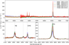 |
Fig. 4. P200/DBSP spectrum observed in February 2018 (orange) and February 2020 (gray) and the YFOSC spectrum observed in April 2020 (green), January 2021 (red), and May 2021 (cyan) in comparison with the archival SDSS spectrum taken in 2002 (blue). Lower panel: a zoomed-in view of the starlight-subtracted and continuum-subtracted spectra in the Hβ and Hα regions, which are calibrated using the [O III] narrow-line flux. |
To further explore the Hα profile changes, we performed detailed spectral fittings to measure the AGN continuum and the emission lines. Firstly, the Galactic extinction was dereddened using the dust map provided by Schlegel et al. (1998). We then tried to decompose the spectra into a host galaxy and AGN component with the principal component analysis method (Yip et al. 2004). However, we obtained negative flux for the host galaxy, which means the spectra are entirely dominated by the AGN emission. Therefore, we did not consider the host galaxy component in our following spectral analysis. The continuum was then modeled by a power law plus a third-order polynomial with the region around the broad emission lines (BELs) masked out, while the optical and UV Fe II were modeled by empirical templates from the literature (Boroson & Green 1992; Vestergaard & Wilkes 2001). For the Balmer emission lines, Drake et al. (2011) found that there are three significant components with narrow, medium, and broad velocity widths. We therefore used three Gaussians to model the Hα (and Hβ) line. For [O III] doublets, each narrow line is fitted by two Gaussians, while that of [N II] and [S II] doublets is represented by a single Gaussian. During spectral fittings, the profiles and redshifts of narrow lines are tied. In addition, flux ratios of the [O III] doublets λ5007, λ4959 and [N II] λ6583, λ6548 are fixed to their theoretical values.
Considering the lower S/N in the Hβ region of the P18 and Y20 spectra, the upper limit on the full width at half maximum (FWHM) of the Hβ broad component is bounded and set by that of Hα. The narrow line components of Balmer lines are assumed to be constant and fixed to those of the preflare SDSS spectrum. The median flux between rest-frame 5095 and 5105 Å is taken to calculate the 5100 Å luminosity.
Uncertainties on the spectral parameters, including the 5100 Å luminosity, were derived using Monte Carlo simulations, where the observed spectrum was randomly perturbed by adding Gaussian noise at each wavelength bin, with amplitude determined by the flux error. This was repeated 100 times, resulting in a distribution of the best-fitting parameter of interest, the standard deviation of which was considered as its 1σ error.
Figure 5 presents the spectral decompositions of Hα line observed in six epochs. The emission-line spectral fitting results are shown in Table 3. Interestingly, we find that the broad and intermediate components of Hα emission line observed with P200 in 2018 show a slight increase in flux with respect to the SDSS ones. The flux for both components rises to a peak in 2020, which is by a factor of ∼3.3 and ∼2.9 higher than that observed with SDSS, respectively (Table 3). Although the actual time for the onset of Hα strengthening is not known, it remains strong at least for ∼2 months based on the current data.
 |
Fig. 5. Illustration of the emission-line-profile fitting in the Hα+[N II] region observed at different epochs. |
Spectroscopic observations and emission-line-fitting results.
Our recent YFOSC spectrum taken in January 2021 and May 2021 shows that the broad Hα flux appears to have declined, though it is still a factor of ∼2 higher than that of the pre-flare SDSS spectrum. This strongly suggests that the Hα brightening is a transient phenomenon. We argue that such an Hα flux variation is not due to observational effects, as our simulations (see the details in Appendix A) have demonstrated that the changes in the Hα EW are at most at a level of 7% under the conditions of five spectroscopic observations (Table 3), i.e., for the seeing between 1.5″ and 3.3″, and the slit width between 1.5″ and 2.5″. Timely spectroscopy monitoring observations are highly encouraged to determine how long the Hα brightening will last.
As the optical BELs are believed to arise largely from the high-density gas clouds in broad line regions (BLRs) that are photoionized by an intense central continuum radiation, we would naively expect correlated changes in the BEL strengths with the intrinsic variations in the incident ionizing continuum flux. This unique property between the continuum and emission line variations constitutes the foundation of the reverberation mapping (RM; see Blandford & McKee 1982) technique, and has proven observationally extremely useful to probe the spatial distribution and kinematics of the BEL gas (see Peterson 1993 and references therein). Greene & Ho (2005) found that the luminosity of Hα BEL is correlated with the continuum luminosity at 5100 Å for an ensemble of AGNs. The best-fit relation suggests  , with an rms scatter of ∼0.2 dex (Greene & Ho 2005). Assuming CSS1029 follows this relation, the observed enhancement in the Hα flux (combined broad and intermediate components) in 2020 by a factor of ∼1.8 in CSS1029 with respect to that of 2018 would indicate a corresponding increase in the 5100Å continuum flux by ∼0.6 ± 0.5 mag.
However, the actual 5100 Å luminosity appears to undergo little change with time during our follow-up spectroscopy observing campaign, as shown in Table 3 and Fig. 6. Such a reverse evolution between the Hα line and continuum variations is even extreme if compared with the pre-flare SDSS spectrum.
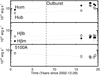 |
Fig. 6. Variation of Hα, Hβ, and the continuum luminosity at 5100 Å as a function of time. Both broad and intermediate emission line components are shown. The dashed vertical line indicates the time of peak luminosity of optical outburst observed on Feb 23 2010 (D11). |
Strictly speaking, the above comparison is unfair because the flux responsivity of Hα BELs to the continuum variations in individual AGNs might be different from the above luminosity–luminosity relation, as in AGNs with RM observations for which the line responsivity typically has a scatter of less than 0.15 dex (e.g., Shapovalova et al. 2012; Shapovalova & Popović 2019). To take into account this effect, we compare in Fig. 7 the variability of Hα BELs with the continuum variability of CSS1029 at g-band observed by ZTF, which has the best sampling in the light curve covering our follow-up spectroscopic observations (thick vertical lines). For clarity, the Hα light curves have been normalized to the mean value of g-band flux at the date of our P18 observation. It can be seen that while the g-band flux remains constant with little evolution over time, the variability amplitudes for Hα BELs are much larger, above the 3σ upper limit on the g-band variability. Under the assumption of  in the RM model, the result clearly suggests that the Hα BEL variability in CSS1029 is not relevant to the continuum variation.
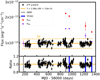 |
Fig. 7. Comparison between the variation in the Hα broad line (purple) and that in medium width component (red) and the observed g-band continuum light curve (black points, see also Fig. 8). The orange solid line represents the linear fit, suggesting that the g-band flux variability can be described by a constant with little evolution over time. The dashed line indicates the 3σ scatter of flux variability relative to its mean. For clarity, the Hα flux has been normalized to the mean g-band flux on the date of Feb 24 2018, the start of our follow-up spectroscopic observations (thick vertical lines). Bottom panel: ratios of the g-band fluxes to the best-fit mean. |
3.5. Multi-wavelength photometric light curves
CSS1029 was discovered by the CRTS survey in February 2010 (D11), but only optical photometry up to ∼300 days post-outburst is shown. We retrieved the optical V-band photometric data from the CRTS website3 and updated to match the long-term light curve as presented in Graham et al. (2017). The V-band light curve is displayed in Fig. 8. It can be seen that the source clearly displays two distinct states in the optical band: a long quiescent state and an outburst state which differs in brightness by ∼1.5–1.8 mag. The quiescent brightness decreases by ∼0.3 mag after the outburst, suggesting a slight change in the accretion rate. In addition, we built MIR light curves by collecting photometric data at 3.4 μm (W1) and 4.6 μm (W2) from the WISE (Wide-field Infrared Survey Explorer) survey up to December 2020. Details of the WISE photometry and light-curve construction are given in Jiang et al. (2016a, 2019a). The MIR flares are clearly presented soon after the optical outburst (MJD 55325), probably due to the dust-reprocessed emission from the circumnuclear region. The MIR flare is followed by a fading back to a long quiescent level, similar to that observed in the optical. The trend is confirmed with the recent g-band light curve from the ZTF (Zwicky Transient Facility) survey4, which displays a plateau over a period of ∼3 years (up to May 2021). We also show the long-term X-ray and UV light curves observed by Swift, though the sampling of the data is much poorer.
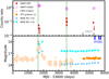 |
Fig. 8. Multi-wavelength light curves showing the changes in continuum over the past 15 years for CSS1029. Upper panel: UV (magenta) and X-ray (red) light curves observed from Swift. Bottom panel: light curve in the optical V-band from the CRTS DR2 (light orange), g-band from the ZTF DR2 (dark orange), and in the MIR 3.4 μm (cyan) and 4.6 μm (light blue) from WISE. The green dashed line represents the time of optical peak in 2010, and the X-ray peak in 2015, respectively. The gray thick lines show the time of our DBSP spectroscopy observations, while the blue thick lines indicate the time of YFOSC spectroscopy observations. |
3.5.1. Analysis of UV to optical SED during outburst
We fitted a blackbody model ( ) to the UV-to-optical photometric data from the Swift UVOT observations during the period of optical burst to put constraints on the luminosity, temperature, and radius evolution of UV and optical emission of CSS1029. Swift UVOT observations cover a wavelength range from ∼1900Å to 5500Å, which is sensitive to the UV-to-optical SED of typical optical TDEs (e.g., van Velzen et al. 2021). In addition, the simultaneous UVOT observations at six filters are helpful in migrating the uncertainties on SED fittings due to the variability in individual bands. We utilized the archival as well as our own target-of-opportunity Swift observations performed in January 2020 and February 2020 to estimate the quiescent host emission. The host emission at each filter is estimated as the mean of flux between the two epochs, which was then subtracted from the total UVOT measurements to obtain the transient photometry during the period of the outburst (and the errors on host flux were propagated). The transient photometry was then corrected for the Galactic extinction of E(B − V) = 0.015 mag (Drake et al. 2011).
We find that the host-subtracted, Galactic extinction-corrected UV-to-optical SED of CSS1029 can be well described by the blackbody model with a reduced χ2/d.o.f. of ∼0.8–0.9 (see Appendix B for the fitting results).
The SED-fitting results indicate a flat evolution of blackbody temperature between ∼40 and 90 days post-optical-peak, with a mean temperature of ∼1.03 × 10⁴ K, as shown in the blue curve in Fig. 9 (upper panel). We note that the temperature fit to the UV-to-optical SED is very sensitive to internal extinction. Although Drake et al. (2011) suggest that the host-galaxy extinction of CSS1029 is a small effect, we estimate a potential internal extinction with the narrow line Balmer decrement as measured from the preflare SDSS spectrum (Drake et al. 2011). By summing the Galactic extinction, we find a total extinction of EB − V = 0.073 assuming an “average” reddening for the diffuse interstellar medium of R(V) = 3.1. Correcting for the total extinction to the UV-optical SED observed by Swift, the best-fit temperature increases to ∼1.13 × 10⁴ K (purple curve in Fig. 9, upper panel), in good agreement with the blackbody component seen in the spectra (Drake et al. 2011). By comparing with the average trend of temperature evolution of the hydrogen-poor superluminous supernovae (SLSNe I) and type II SNe (e.g., Inserra et al. 2018), we find that CSS1029 displays a considerably higher temperature (by a factor of ∼1.5) than the SNe at the same epoch (∼40–90 days post-peak). The dramatic temperature evolution for the SNe is likely resulting from cooling due to rapid expansion and radiative losses.
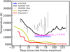 |
Fig. 9. Temperature evolution of UV-optical emission of CSS1029 compared with that of SLSNe and type II SNe (Inserra et al. 2018). The blue curve shows the blackbody temperature measured from the photometric data corrected for the Galactic dust extinction (EB − V = 0.015), while the purple curve represents that corrected for both the Galactic and internal dust extinction (EB − V = 0.073). The latter is estimated from the Balmer decrement of narrow emission lines (Drake et al. 2011). The temperature evolution of CSS1029 appears similar to that of optical TDE ASASSN-14ae (gray points, Holoien et al. 2014), as well as the peculiar SLSN ASASSN-15lh (black curve, Dong et al. 2016). The latter has been suggested to be more consistent with a TDE based on recent observations (Leloudas et al. 2016). |
3.5.2. MOSFIT fittings to the optical light curve of outburst
We further explored whether the optical light curve of outburst can be fitted with the Monte Carlo software MOSFIT, which was recently applied to model the light curves of TDEs (Mockler et al. 2019). This was not done in previous work (D11). The TDE model in MOSFIT assumes that emission produced within an elliptical accretion disk of a TDE is partly reprocessed into the UV/optical by an optically thick layer (Guillochon et al. 2018). We run MOSFIT using a variant of the emcee ensemble-based Markov chain Monte Carlo routine until the fit has converged by reaching a potential scale reduction factor of < 1.2 (Mockler et al. 2019). In Fig. 10, we show the host-subtracted V-band light curve, and an ensemble of model realizations from MOSFIT. The model is able to reproduce the data quite well, including the stages of the rise to peak, near the peak, and the steady decline at later times.
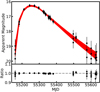 |
Fig. 10. Host-subtracted V-band light curve of CSS1029 (filled circles), and the best model realizations from MOSFIT (red curves). The most relevant best-fit model parameters are listed in Table 4. |
MOSFIT uses the Watanabe-Akaike information criterion (WAIC; Gelman et al. 2014)5 to quantify how well the various combinations of parameters in the modeling fit the data. For CSS1029, we find WAIC = 119, which is fairly consistent with the best-fit values for a sample of optical TDEs (Mockler et al. 2019), suggesting that the fitting result is acceptable.
The best-fit parameters of the TDE model with the corresponding systematic and statistical errors at 1σ confidence are shown in Table 4. Figure 11 shows the posterior probability distribution of the most relevant model parameters in the fit. The best-fit model is that of a black hole of 2.1 × 10⁷ M⊙ disrupting a star of 0.98 M⊙. This black hole mass is consistent within errors with the mass estimated by Blanchard et al. (2017) using the Hα BEL. In comparison with other TDEs modeled in Mockler et al. (2019), the stellar mass for CSS1029 is larger than most other TDEs where a disrupted star with mass near 0.1 M⊙ is preferred. As Table 4 shows, the best-fit model from MOSFIT indicates that the star was likely partially disrupted as the impact parameter b < 1 (Mockler et al. 2019). This is similar to the case in the TDE AT2018hyz (Gomez et al. 2020), which has a b = 0.4.
 |
Fig. 11. Posterior distributions of model parameters from the fit to the V-band light curve of CSS1029 shown in Fig. 10. The contours (from inside to outside) indicate the 1σ and 2σ confidence intervals for two parameters of interest, respectively. |
Best-fit model parameters from MOSFIT.
4. Discussion and conclusion
4.1. Nature of optical outburst
Since its discovery, the nature of the optical outburst shown in the CRTS V-band light curve (Fig. 8) has been disputed. D11 explored an origin of optical outburst as an AGN flare, a TDE, or a Type IIn SLSN, and argued for the last option, which has to occur within 150 pc of the nucleus of the galaxy. The normal AGN variability was ruled out as such a rapid (duration of ∼1 yr), energetic optical flare (total integrated energy of ∼1052 erg) is rarely seen in the light curves of NSy1s (D11; Kankare et al. 2017).
On the other hand, the MIR outbursts in CSS1029 are clearly detected with WISE.
In both the cases of SNe and TDE, strong MIR flares are generally thought to be thermal emission from the dust heated by the nuclear optical outburst. The optical emission from the outburst can sublimate the dust within a certain range and form a dust cavity, the radius of which can be described by the sublimation radius rsub. Assuming a dust sublimation temperature of 1800 K and a grain radius of 0.1 μm, the peak bolometric luminosity of the outburst of 4 × 1044 erg s−1 in CSS1029 suggests a rsub of ∼0.3 light years6. The IR-emitting dust has a distance r ≳ rsub from the central source, causing the IR emission to be delayed relative to the optical emission. If the dust is heated directly by central UV/optical radiation, the time delay τ ∼ r/c would be expected to be several months. Conversely, if the dust is shock-heated by the material moving outward at a speed of vout (typically ∼0.02–0.1 c) from either the ejecta for SNe or outflow for TDE, the time delay τ ∼ r/vout would be several years or longer. As the MIR outburst in CSS1029 was detected several months after the optical peak, the dust should be heated directly by radiation. The possibility that nonthermal radiation from a relativistic jet is causing the MIR flare can be ruled out, because the galaxy is radio quiet (f6 cm/4400 Å ≲ 1, D11). The host-subtracted peak MIR luminosity of CSS1029 is as high as 1.26 × 1044 erg s−1. As shown in Fig. 12, the peak MIR luminosity is among the brightest seen for MIR nuclear transients, which is about two orders of magnitude higher than typical SNe explosions (Jiang et al. 2019a, 2021; Szalai et al. 2019), and one order of magnitude higher than the rare population of SLSNe explosions, such as ASASSN-15lh (Dong et al. 2016). The peak MIR luminosity is close to those of several TDE candidates, including F01004-2237 (Dou et al. 2017), Arp 299B-AT1 (Mattila et al. 2018), and PS1-10adi (Jiang et al. 2019a). Thus, the high MIR luminosity most favors the TDE interpretation of the outburst.
 |
Fig. 12. Host-subtracted WISE W2 (4.6 μm) magnitude for CSS1029 during outburst. For comparison, we also plot the evolution of the peak MIR luminosity of the TDE F01004-2237 (Dou et al. 2017) and PS16dtm (Blanchard et al. 2017), SLSNe (Jiang et al. 2019a), and the supernovae with an excess of MIR emission, i.e., Type Iax SN 2014dt (Fox et al. 2016). |
We note that because of the sparse sampling of the MIR photometry during the outburst phase, the true peak luminosity for CSS1029 may be even higher. Furthermore, the optical peak luminosity matches the Eddington luminosity of the SMBH (Blanchard et al. 2017), supporting its association with accretion.
In Sect. 3.5.1, we show that CSS1029 exhibits a roughly constant temperature of T ≃ 11 300 K between ∼40 and 90 days post-optical-peak. This is neither expected from the photosphere evolution of type II SNe, nor observed for hydrogen-poor SLSN (Inserra et al. 2018). For a typical SNe, both its temperature and bolometric luminosity drop roughly as power laws with time during the early stage (∼1−3 weeks), possibly as a result of cooling due to rapid expansion and radiative losses (e.g., Faran et al. 2018). Once the hydrogen recombination becomes important, which dominates the drop in the optical depth of the photosphere expansion, the temperature remains almost constant at ∼6000–7000 K. With a temperature that is higher than that of the average SN by a factor of ∼1.5 at the same epoch (Fig. 9), this suggests that CSS1029 might be different from typical SNe explosions. However, the TDE candidate ASASSN-14ae showed a very similar temperature evolution to CSS1029. In fact, most TDEs discovered in the optical bands exhibit a relatively flat temperature evolution over several months post-peak (van Velzen et al. 2021; Holoien et al. 2021). The constant temperature evolution could be explained if the UV and optical emission are powered by the reprocessed accretion radiation by unbound TDE outflow (Metzger & Stone 2016). This similarity between the evolution of CSS1029 and TDEs suggests that they might be due to the same mechanism.
On the other hand, the temperature for CSS1029 is at the low end of the temperature range observed for TDEs (of ∼1−4 × 10⁴ K). van Velzen et al. (2021) found a significant anti-correlation between the blackbody radius and temperature, following the relation Lbb ∝ R2T4. By fitting to the UV-to-optical SED, we find that the blackbody radius of CSS1029 is ∼6−8 × 1015 cm (Fig. B.2), which is at the high end of the radius range observed for TDEs (Holoien et al. 2021). If assuming that the blackbody photospheric radius is proportional to the size of the accretion disk in the context of TDEs, the large blackbody radius of CSS1029 could be attributed to the higher mass of the disrupted star (van Velzen et al. 2021). This is consistent with the results of MOSFIT fittings to the V-band light curve (Table 4), where a black hole of 2 × 10⁷ M⊙ disrupting a star of 0.98 M⊙ is inferred.
We note that D11 argued against a TDE explanation primarily because the blackbody temperature and flux decline rate were inconsistent with theoretical predictions from early studies of TDEs. However, as shown in Sect. 3.1, the exponential decline rate that can best describe the outburst evolution of CSS1029 has also been observed in many TDEs that are discovered in modern optical surveys (e.g., Holoien et al. 2014, 2016; Shu et al. 2020). In addition, as shown in Sect. 3.4, our spectroscopy follow-up observations reveal a brightening of the broad Hα flux about a decade after the optical outburst. Although a broad Hα emission component has been observed to emerge in the late-time spectra of some SLSNes (Gal-Yam 2019), the timescale for the appearance is much shorter, of typically ∼1 yr. This makes the origin of late-time Hα brightening in CSS1029 distinct from what is expected in SLSNe, and likely related to a TDE. Given the high peak MIR luminosity and relatively constant temperature evolution of T ∼ 11000 K over ∼40–90 days post-optical-peak, we conclude that a TDE origin is preferred for the optical outburst for CSS1029 and the scenario with a superluminous SNe explosion seems disfavored.
4.2. Possible origins for the X-ray brightening
By analyzing the follow-up observations with Swift taken in 2015 and 2020, we find an X-ray brightening of ≳30 in CSS1029 relative to its previous low state in 2010, followed by a flux fading within about two weeks. The appearance of bright X-ray emission at later times and its rapid decline in flux within a short period appear to be an unusual property of CSS1029. As it was established previously that the optical spectrum of CSS1029 is that of NSy1 (D11), this may suggest that the X-ray brightening could be attributed to the AGN activity. This is supported by the detection of a hard X-ray component with 2–10 keV luminosity of  (Sect. 3.2), and a best-fit photon index of Γ ∼ 2.1, which is typical for NSy1s. However, we note that the large-amplitude X-ray variability in CSS1029 is probably distinct from the rapid AGN variability seen on shorter timescales of hours to days (e.g., Uttley et al. 1999)7.
As mentioned in Sect. 3.3, the UV emission shows little variability during the X-ray flaring, with maximum variability amplitude of ∼50%, which is mild compared with the X-ray one. Moreover, as shown in Fig. 8, we do not find any coincident variability in either optical or MIR with the X-ray flaring in 2015. We note that similar X-ray flares have been observed in the AGN IC 3599 which could be attributed to an instability in a radiation-pressure-dominated accretion disk (Grupe et al. 2015), or multiple tidal disruption flares with the recurrence time of 9.5 yr (Campana et al. 2015). However, in this case, a large optical outburst was also observed prior to the X-ray one, making it physically different from what is observed in CSS1029.
This suggests that the scenario whereby a dramatic change in AGN accretion rate is causing the extreme X-ray variability in CSS1029 is unlikely. Microlensing by stars in foreground galaxies also seems unable to explain the observed X-ray behavior, as the model predicts a variability that is independent of wavelengths (e.g., Lawrence et al. 2016).
The apparent lack of coincident optical/UV variability with X-ray flaring in CSS1029 is somewhat similar to that found in some NSy1s with extreme X-ray variations (e.g., Bachev et al. 2009; Miniutti et al. 2012; Grupe et al. 2008, 2019; Buisson et al. 2018). It has been suggested that the absorber with a nonunity covering fraction at large scale can cause the X-ray variability, but it is required to be dust-free so as not to affect the UV or optical emission. Assuming a single large cloud passing over the X-ray source, we can use the observed duration of the decline in X-ray flux in 2015 (at least 10 d, Table 1) to constrain the location of the absorber. The crossing time for an intervening cloud on a Keplerian orbit can be estimated as

where rc is the distance of the cloud to the X-ray source, Dsrc is the size of the X-ray source, and tcross ≈ Dsrc/VK, where VK is Keplerian velocity (Risaliti et al. 2007). For a BH mass of 7.9 × 10⁶ M⊙ (Blanchard et al. 2017) and a typical diameter of 10RG for the X-ray source (e.g., Fabian et al. 2009), we find the location of the intervening cloud to be rc ≳ 5 × 1018 cm in order to have an obscuration that lasts longer than 10 d. This corresponds to ∼1.6 pc, which is suggestive of a cloud that lies outside of the BLR. We note that this distance is much larger than the typical dust sublimation radius in AGNs (∼0.1 pc, Jiang et al. 2019a), making the explanation for the presence of dust-free clouds at such a large distance challenging. Therefore, the scenario whereby the X-ray brightening in CSS1029 is due to the movement of dust-free absorbing gas at large scale seems disfavored.
Having established that TDE could plausibly power the optical outburst, we discuss the possibility of whether a TDE could contribute to the X-ray variability in CSS1029. Hydrodynamics simulations have shown that the debris stream of a TDE can affect the accretion properties of pre-existing AGNs (Chan et al. 2019). Blanchard et al. (2017) presented the observation of PS16dtm, a TDE occurring at the nucleus of a NSy1, which shares many similarities with CSS1029. Blanchard et al. (2017) suggested that the TDE can lead to dimming of the X-ray emission from the pre-existing AGN, possibly due to obscuration of the X-ray-emitting region by stellar debris. These latter authors further predicted that the source will become X-ray bright again approximately a decade after the TDE, though this has not yet been confirmed. In comparison with PS16dtm, the relatively faint X-ray flux of CSS1029 observed in 2010 could simply be due to partial obscuration of the X-ray-emitting region by accreting stellar debris, and the brightening in 2015 could be attributed to a decrease in the optical depth of the absorbing gas as the accretion rate declines.
On the other hand, Ricci et al. (2020) found clear evidence that the hard power-law component (produced in the X-ray corona) disappeared after the UV and optical outbursts in the AGN 1ES1927+65, i.e., drops in luminosity by more than three orders of magnitude. Interestingly, such a power-law component reappeared about one year later. Ricci et al. (2020) invoked the TDE scenario to explain the drastic X-ray variability, which can deplete the innermost regions of accretion flow (Chan et al. 2019), hence disrupting the magnetic field powering the X-ray corona. If the relative X-ray faintness of CSS1029 in 2010 is due to the destruction of AGN X-ray corona, its X-ray luminosity (L0.3−2 keV ∼ 3.7 × 1042 erg s−1) appears too high in comparison to what is observed in 1ES1927+65. In this case, the observed X-ray emission of CSS1029 in 2010 could be attributed entirely to the TDE.
Alternatively, several authors have invoked a partial covering model to account for extreme X-ray variability behaviors in AGNs, especially those high-accreting systems (Luo et al. 2015; Liu et al. 2019; Ni et al. 2020). In this model, the central X-ray source could be partially obscured by a thick inner disk or outflow if it intercepts the line of sight.
A similar scenario was proposed to explain the faintness of the X-ray emission in optical TDEs involving the orientation effect where the X-rays from the inner disk are obscured by dense outflow gas (Dai et al. 2018). The slight changes in the covering factor with respect to the X-ray source would result in an X-ray variability, but the bulk UV and optical continuum at the outer disk remains little affected. Indeed, Blanchard et al. (2017) estimated that the Eddington ratio is close to 1 for CSS1029 when it reaches to the peak luminosity of outburst in 2010, indicating that the central BH is accreting at a high rate during this epoch. Simulations suggest that geometrically thick inner accretion disks and associated dense outflows will be formed when the accretion rate is high enough (Jiang et al. 2014, 2019b).
This is suggestive of the possibility that a thick disk in the inner region formed in CSS1029 plays a role in partially obscuring the central X-ray source, explaining the low X-ray flux observed in 2010. The X-ray brightening observed at later times may be due to a decrease in the thickness or covering factor of the inner disk with accretion rate (radiation luminosity), possibly induced by the TDE process. As shown in Fig. 8, the baseline AGN optical emission decrease by a factor of ∼0.3 mag after the outburst seems to be in accordance with this scenario.
4.3. Hα anomaly and implications for BLR evolution
In Sect. 3.4, our analysis suggests transient Hα brightening in CSS1029 that might not be relevant to the continuum variation. Although we cannot locate spectra taken between 2018 and 2020, the most recent photometric observations by Swift show that the amplitude of continuum variability at UV and optical bands was not as large as that expected from the Hα brightening (Table 1). The lack of corresponding ionizing continuum variability is further supported by the WISE light curves at MIR bands (Fig. 8), which suggest no recent outburst even for the largely unobservable extreme-UV variation up to December 2020; otherwise, an MIR echo signal might be detected.
We argue that the “nonresponsivity” of ionizing continuum variability is not due to the contamination of the constant host emission, as the optical continuum is dominated by the AGN emission in the spectroscopic data (Sect. 3.4). The clear flux decline in the V-band light curve by ∼0.3 mag (Fig. 8) also suggests that the optical flux is dominated by the AGN emission.
Therefore, the observed Hα brightening is an anomalous behavior of the BEL variations in the context of the RM model. We note that such a transient anomalous phenomenon has been reported in other AGNs from the RM campaign (Goad et al. 2016; Gaskell et al. 2021), but most are characterized by a significant deficit in the flux of BELs when the continuum is brightened, which is clearly different from the Hα anomaly observed in CSS1029.
As no clear evidence for a temporary increase in the ionizing continuum incident upon BLR clouds is found during or before the anomaly, it could be possible to explain the enhanced Hα emission by an increase in gas density or excitation within the BLR itself. Although the formation processes of the BLR are still unknown, Czerny & Hryniewicz (2011) suggested that the BLR is a failed dusty wind from the outer accretion disk. Baskin & Laor (2018) refined this model by exploring the dust properties and implied the BLR structure in more detail, and proposed a dust-inflated accretion disk as the origin of the BLR. The dusty disk wind scenario may not be able to explain the Hα anomaly, as it requires a replenishment of dusty clouds emerging from the accretion disk resulting in a brightening in the IR emission before the Hα enhancement, which is not yet observed. On the other hand, Wang et al. (2017) suggested that tidally disrupted clumps within the dust sublimation radius of the torus by the central black hole may become bound at smaller radii to serve as the source of the BLR gas. In such a model, the Hα anomaly in CSS1029 could be induced by a sudden increase in the tidal disruption rate, or in the total mass of tidally disrupted clumps, supplying as addition to the BLR gas clouds. However, the mechanism by which the tidal disruption rate is increased abruptly is not clear in this scenario. In addition, one would ask why the similar behavior of the BEL variations has not been observed in other AGNs for which intense RM monitoring campaigns are available.
As we demonstrate above, CSS1029 represents one of the few AGNs in which a TDE-like energetic transient event has been discovered (e.g., Kankare et al. 2017; Blanchard et al. 2017; Shu et al. 2018; Liu et al. 2020). While the stellar disruption itself may be less affected by the AGN accretion disk, the bound debris stream could collide with the disk, exciting shocks and leading to inflow and considerable energy dissipation in the disk as well as the coronal region responsible for most of the AGN X-ray emission (Blanchard et al. 2017; Chan et al. 2019; Ricci et al. 2020). On the other hand, it has been proposed that when a star is disrupted, roughly half the stellar debris is unbound, and ejected with an estimated velocity of  (Evans & Kochanek 1989). In the context of TDE, for a solar-type star disrupted by a black hole of MBH = 7.9 × 10⁶ M⊙ in CSS1029 (Sect. 4.3), the maximum ejection velocity is of vej ∼ 8 × 10³ km s−1. The ejection of unbound debris may run into the BLR, providing an alternative supply for the BLR gas to explain the Hα anomaly. Indeed, the geometry and energetics of the ejected material and possible observational consequences of the interaction of this material with the ambient medium surrounding the black hole have been investigated theoretically (Rees 1988; Kochanek 1994; Khokhlov & Melia 1996; Guillochon et al. 2016). Given an expected BLR size of rBLR ∼ 30 light days from the 5100 Å luminosity, the timescale for debris to spread out and reach the BLR is rBLR/vej = 3.1 years. However, TDE simulations have shown that the average kinetic energy for ejecta is about an order of magnitude lower than expected, resulting in a typical outgoing velocity of ∼2500 km s−1 (Guillochon & Ramirez-Ruiz 2013). This corresponds to a timescale of ∼10 years for debris moving to the BLR, which is not inconsistent with the time when the Hα enhancement was observed in CSS1029. It is intriguing to note that the changes in the flux of the higher order Hβ line are less than those of Hα (Fig. 6), indicating that the gas replenishment alone may not be able to account for the spectral evolution of CSS1029, as a larger responsivity of Hβ is expected with decreasing ionization parameter (Korista & Goad 2004). This suggests that in addition to photoionization, collisional excitation might be important for producing Hα. Better quantitative modeling of the interaction of stellar debris with the BLR might be required to explain the anomalous enhancement of Hα emission, which is beyond the scope of this paper.
As an anomalous behavior of this kind in BEL variation is rare in AGNs, spectroscopic monitoring campaigns of CSS1029 with contemporaneous multi-wavelength photometric observations are encouraged. In addition, observations of similar BEL anomalies in other AGNs from dedicated RM campaigns are important to decipher whether this is unique for CSS1029 (e.g., due to the TDE influence) or is a common phenomenon among AGNs. Such datasets could potentially reveal the underlying physical processes that drive the (de)correlation between continuum and BEL variations, yielding new insights into the formation and evolution of BLRs.
Since the 1σ detection from the background fluctuation results in less than one net count, we estimated conservatively the upper limit by requiring the detection of one net count, as did in Shu et al. (2020).
αox, exp is the αox expected from the Grupe et al. (2010)αox − L2500 Å relation.
Here we used the formula given in Namekata & Umemura (2016) to estimate the sublimation radius

From the extinction-corrected [O III]λ5007 luminosity of 2.4 × 1041erg s−1 from the SDSS spectrum (D11), we roughly estimated the “time-averaged” 2–10 keV luminosity of 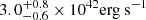 (e.g., Lamastra et al. 2009). This is a factor of ∼3 higher than the upper limit of hard X-ray luminosity obtained in 2010, suggesting that CSS1029 could be in a historically low X-ray state during the optical outburst.
Acknowledgments
We thank the Swift Acting PI, Brad Cenko, for approving our ToO request to observe CSS1029, Matthew J. Graham, Andrew J. Drake for kindly providing the post-DR2 CRTS data for the source, and Pu Du for timely coordinating the Lijiang/YFOSC observations. This research made use of the HEASARC online data archive services, and data products from the Wide-field Infrared Survey Explorer, Catalina Real-time Transient Survey and Zwicky Transient Facility Project. We acknowledge the use of the Hale 200-inch Telescope through the Telescope Access Program (TAP), under the agreement between the National Astronomical Observatories, CAS, and the California Institute of Technology, and the support of the staff of the Lijiang 2.4 m telescope. Funding for the Lijiang telescope has been provided by CAS and the People’s Government of Yunnan Province. This work is supported by Chinese NSF through grant Nos. 11822301, 12192220, 12192221, 11833007, U1931131, U1731104, and the science research grants from the China Manned Space Project with No. CMS-CSST-2021-A06.
References
- Auchettl, K., Guillochon, J., & Ramirez-Ruiz, E. 2017, ApJ, 838, 149 [Google Scholar]
- Auchettl, K., Ramirez-Ruiz, E., & Guillochon, J. 2018, ApJ, 852, 37 [NASA ADS] [CrossRef] [Google Scholar]
- Bachev, R., Grupe, D., Boeva, S., et al. 2009, MNRAS, 399, 750 [NASA ADS] [CrossRef] [Google Scholar]
- Baskin, A., & Laor, A. 2018, MNRAS, 474, 1970 [Google Scholar]
- Blandford, R. D., & McKee, C. F. 1982, ApJ, 255, 419 [Google Scholar]
- Blanchard, P., Nicholl, M., Berger, E., & Guillochon, J. 2017, ApJ, 843, 106 [NASA ADS] [CrossRef] [Google Scholar]
- Boller, T., Schmitt, J. H. M. M., Buchner, J., et al. 2022, A&A, in press, https://doi.org/10.1051/0004-6361/202141155 [Google Scholar]
- Boroson, T. A., & Green, R. F. 1992, ApJS, 80, 109 [Google Scholar]
- Buisson, D. J. K., Lohfink, A. M., Alston, W. N., et al. 2018, MNRAS, 475, 2306 [NASA ADS] [CrossRef] [Google Scholar]
- Campana, S., Mainetti, D., Colpi, M., et al. 2015, A&A, 581, A17 [NASA ADS] [CrossRef] [EDP Sciences] [Google Scholar]
- Chan, C.-H., Piran, T., Krolik, J. H., et al. 2019, ApJ, 881, 113 [NASA ADS] [CrossRef] [Google Scholar]
- Czerny, B., & Hryniewicz, K. 2011, A&A, 525, L8 [NASA ADS] [CrossRef] [EDP Sciences] [Google Scholar]
- Dai, L., McKinney, J. C., Roth, N., et al. 2018, ApJ, 859, L20 [NASA ADS] [CrossRef] [Google Scholar]
- Dong, S., Shappee, B. J., Prieto, J. L., et al. 2016, Science, 351, 257 [NASA ADS] [CrossRef] [Google Scholar]
- Dou, L., Wang, T., Yan, L., et al. 2017, ApJ, 841, L8 [Google Scholar]
- Drake, A. J., Djorgovski, S. G., Mahabal, A., et al. 2009, ApJ, 696, 870 [Google Scholar]
- Drake, A. J., Djorgovski, S. G., Mahabal, A., et al. 2011, ApJ, 735, 106 [NASA ADS] [CrossRef] [Google Scholar]
- Elvis, M., Wilkes, B. J., McDowell, J. C., et al. 1994, ApJS, 95, 1 [Google Scholar]
- Evans, C. R., & Kochanek, C. S. 1989, ApJ, 346, L13 [Google Scholar]
- Fabian, A. C., Zoghbi, A., Ross, R. R., et al. 2009, Nature, 459, 540 [Google Scholar]
- Fabian, A. C., Zoghbi, A., Wilkins, D., et al. 2012, MNRAS, 419, 116 [Google Scholar]
- Fabian, A., Parker, M., Wilkins, D., & Miller, J. 2014, MNRAS, 439, 2307 [NASA ADS] [CrossRef] [Google Scholar]
- Faran, T., Nakar, E., & Poznanski, D. 2018, MNRAS, 473, 513 [NASA ADS] [CrossRef] [Google Scholar]
- Fox, O. D., Johansson, J., Kasliwal, M., et al. 2016, ApJ, 816, L13 [Google Scholar]
- Gallo, L. C., Grupe, D., Schartel, N., et al. 2011, MNRAS, 412, 161 [NASA ADS] [CrossRef] [Google Scholar]
- Gal-Yam, A. 2019, ARA&A, 57, 305 [Google Scholar]
- Gaskell, C. M., Bartel, K., Deffner, J. N., et al. 2021, MNRAS, 508, 6077 [NASA ADS] [CrossRef] [Google Scholar]
- Gelman, A., Hwang, J., & Vehtari, A. 2014, Stat. Comput., 24, 997 [Google Scholar]
- Gibson, R. R., Brandt, W. N., & Schneider, D. P. 2008, ApJ, 685, 773 [NASA ADS] [CrossRef] [Google Scholar]
- Gierliński, M., Middleton, M., Ward, M., et al. 2008, Nature, 455, 369 [CrossRef] [Google Scholar]
- Gilli, R., Maiolino, R., Marconi, A., et al. 2000, A&A, 355, 485 [NASA ADS] [Google Scholar]
- Goad, M. R., Korista, K. T., De Rosa, G., et al. 2016, ApJ, 824, 11 [NASA ADS] [CrossRef] [Google Scholar]
- Gomez, S., Nicholl, M., Short, P., et al. 2020, MNRAS, 497, 1925 [NASA ADS] [CrossRef] [Google Scholar]
- González-Martín, O., & Vaughan, S. 2012, A&A, 544, A80 [NASA ADS] [CrossRef] [EDP Sciences] [Google Scholar]
- Graham, M. J., Djorgovski, S. G., Drake, A. J., et al. 2017, MNRAS, 470, 4112 [NASA ADS] [CrossRef] [Google Scholar]
- Greene, J. E., & Ho, L. C. 2005, ApJ, 630, 122 [NASA ADS] [CrossRef] [Google Scholar]
- Grupe, D., Komossa, S., Gallo, L. C., et al. 2008, ApJ, 681, 982 [NASA ADS] [CrossRef] [Google Scholar]
- Grupe, D., Komossa, S., Leighly, K. M., et al. 2010, ApJS, 187, 64 [NASA ADS] [CrossRef] [Google Scholar]
- Grupe, D., Komossa, S., Leighly, K. M., et al. 2012a, Eur. Phys. J. Web Conf., 39, 06001 [NASA ADS] [CrossRef] [EDP Sciences] [Google Scholar]
- Grupe, D., Komossa, S., Gallo, L. C., et al. 2012b, ApJS, 199, 28 [NASA ADS] [CrossRef] [Google Scholar]
- Grupe, D., Komossa, S., & Saxton, R. 2015, ApJ, 803, L28 [NASA ADS] [CrossRef] [Google Scholar]
- Grupe, D., Komossa, S., Gallo, L., & Schartel, N. 2019, MNRAS, 486, 227 [NASA ADS] [Google Scholar]
- Guainazzi, M., Nicastro, F., Fiore, F., et al. 1998, MNRAS, 301, L1 [NASA ADS] [CrossRef] [Google Scholar]
- Guillochon, J., & Ramirez-Ruiz, E. 2013, ApJ, 767, 25 [NASA ADS] [CrossRef] [Google Scholar]
- Guillochon, J., Manukian, H., & Ramirez-Ruiz, E. 2014, ApJ, 783, 23 [NASA ADS] [CrossRef] [Google Scholar]
- Guillochon, J., McCourt, M., Chen, X., et al. 2016, ApJ, 822, 48 [NASA ADS] [CrossRef] [Google Scholar]
- Guillochon, J., Nicholl, M., Villar, V. A., et al. 2018, ApJS, 236, 6 [NASA ADS] [CrossRef] [Google Scholar]
- Hinkle, J. T., Holoien, T. W. S., Shappee, B. J., et al. 2021, AAS J., submitted [arXiv:2108.03245] [Google Scholar]
- Holoien, T. W.-S., Prieto, J. L., Bersier, D., et al. 2014, MNRAS, 445, 3263 [Google Scholar]
- Holoien, T. W.-S., Kochanek, C. S., Prieto, J. L., et al. 2016, MNRAS, 463, 3813 [NASA ADS] [CrossRef] [Google Scholar]
- Holoien, T. W. S., Neustadt, J. M. M., Vallely, P. J., et al. 2021, ApJ, submitted [arXiv:2109.07480] [Google Scholar]
- Inserra, C., Smartt, S. J., Gall, E. E. E., et al. 2018, MNRAS, 475, 1046 [NASA ADS] [CrossRef] [Google Scholar]
- Jiang, Y.-F., Stone, J. M., & Davis, S. W. 2014, ApJ, 796, 106 [NASA ADS] [CrossRef] [Google Scholar]
- Jiang, N., Dou, L., Wang, T., et al. 2016a, ApJ, 828, L14 [Google Scholar]
- Jiang, Y., Davis, S., & Stone, J. 2016b, ApJ, 827, 10J [NASA ADS] [CrossRef] [Google Scholar]
- Jiang, N., Wang, T., Mou, G., et al. 2019a, ApJ, 871, 15 [Google Scholar]
- Jiang, Y.-F., Stone, J. M., & Davis, S. W. 2019b, ApJ, 880, 67 [Google Scholar]
- Jiang, N., Wang, T., Dou, L., et al. 2021, ApJS, 252, 32 [Google Scholar]
- Kankare, E., Kotak, R., Mattila, S., et al. 2017, Nat. Astron., 1, 865 [NASA ADS] [CrossRef] [Google Scholar]
- Karas, V., & Šubr, L. 2007, A&A, 470, 11 [NASA ADS] [CrossRef] [EDP Sciences] [Google Scholar]
- Khokhlov, A., & Melia, F. 1996, ApJ, 457, L61 [NASA ADS] [CrossRef] [Google Scholar]
- Kochanek, C. S. 1994, ApJ, 422, 508 [NASA ADS] [CrossRef] [Google Scholar]
- Komossa, S. 2015, J. High Energy Astrophys., 7, 148 [Google Scholar]
- Korista, K. T., & Goad, M. R. 2004, ApJ, 606, 749 [NASA ADS] [CrossRef] [Google Scholar]
- Lamastra, A., Bianchi, S., Matt, G., et al. 2009, A&A, 504, 73 [NASA ADS] [CrossRef] [EDP Sciences] [Google Scholar]
- Lawrence, A. 2018, Nat. Astron., 2, 102 [NASA ADS] [CrossRef] [Google Scholar]
- Lawrence, A., Bruce, A. G., MacLeod, C., et al. 2016, MNRAS, 463, 296 [NASA ADS] [CrossRef] [Google Scholar]
- Leloudas, G., Fraser, M., Stone, N. C., et al. 2016, Nat. Astron., 1, 0002 [Google Scholar]
- Lin, D., Guillochon, J., Komossa, S., et al. 2017, Nat. Astron., 1, 0033 [Google Scholar]
- Liu, H., Luo, B., & Brandt, W. N. 2019, ApJ, 878, 79 [NASA ADS] [CrossRef] [Google Scholar]
- Liu, Z., Li, D., Liu, H.-Y., et al. 2020, ApJ, 894, 93 [Google Scholar]
- Luo, B., Brandt, W. N., Hall, P. B., Wu, J., & Anderson, S. F. 2015, ApJ, 805, 122 [NASA ADS] [CrossRef] [Google Scholar]
- Mattila, S., Pérez-Torres, M., Efstathiou, A., et al. 2018, Science, 361, 482 [Google Scholar]
- Metzger, B. D., & Stone, N. C. 2016, MNRAS, 461, 948 [NASA ADS] [CrossRef] [Google Scholar]
- Middei, R., Vagnetti, F., Bianchi, S., et al. 2017, A&A, 599, A82 [NASA ADS] [CrossRef] [EDP Sciences] [Google Scholar]
- Miniutti, G., & Fabian, A. 2004, MNRAS, 349, 1435 [NASA ADS] [CrossRef] [Google Scholar]
- Miniutti, G., Fabian, A., Goyder, R., & Lasenby, A. 2003, MNRAS, 344, L22 [NASA ADS] [CrossRef] [Google Scholar]
- Miniutti, G., Brandt, W. N., Schneider, D. P., et al. 2012, MNRAS, 425, 1718 [NASA ADS] [CrossRef] [Google Scholar]
- Miniutti, G., Sanfrutos, M., Beuchert, T., et al. 2014, MNRAS, 437, 1776 [NASA ADS] [CrossRef] [Google Scholar]
- Miniutti, G., Saxton, R. D., Giustini, M., et al. 2019, Nature, 573, 381 [Google Scholar]
- Mockler, B., Guillochon, J., & Ramirez-Ruiz, E. 2019, ApJ, 872, 151 [Google Scholar]
- Namekata, D., & Umemura, M. 2016, MNRAS, 460, 980 [NASA ADS] [CrossRef] [Google Scholar]
- Ni, Q., Brandt, W., Luo, B., Hall, P., & Shen, Y. 2018, MNRAS, 480, 5184 [NASA ADS] [Google Scholar]
- Ni, Q., Brandt, W. N., Yi, W., et al. 2020, ApJ, 889, L37 [NASA ADS] [CrossRef] [Google Scholar]
- Oknyansky, V. L., Winkler, H., Tsygankov, S. S., et al. 2019, MNRAS, 483, 558 [NASA ADS] [CrossRef] [Google Scholar]
- Parker, M. L., Komossa, S., Kollatschny, W., et al. 2016, MNRAS, 461, 1927 [NASA ADS] [CrossRef] [Google Scholar]
- Peterson, B. M. 1993, PASP, 105, 247 [NASA ADS] [CrossRef] [Google Scholar]
- Peterson, B. M., Denney, K. D., De Rosa, G., et al. 2013, ApJ, 779, 109 [NASA ADS] [CrossRef] [Google Scholar]
- Rees, M. J. 1988, Nature, 333, 523 [Google Scholar]
- Ricci, C., Kara, E., Loewenstein, M., et al. 2020, ApJ, 898, L1 [Google Scholar]
- Ricci, C., Loewenstein, M., Kara, E., et al. 2021, ApJS, 255, 7 [NASA ADS] [CrossRef] [Google Scholar]
- Risaliti, G., Elvis, M., Fabbiano, G., Baldi, A., & Zezas, A. 2005, ApJ, 623, L93 [Google Scholar]
- Risaliti, G., Elvis, M., Fabbiano, G., et al. 2007, ApJ, 659, L111 [NASA ADS] [CrossRef] [Google Scholar]
- Saxton, R., Read, A., Esquej, P., et al. 2011, Narrow-line Seyfert 1 Galaxies andTheir Place in the Universe, 8 [Google Scholar]
- Saxton, R. D., Motta, S. E., Komossa, S., et al. 2015, MNRAS, 454, 2798 [NASA ADS] [CrossRef] [Google Scholar]
- Saxton, R., Motch, C., Komossa, S., et al. 2019, Astron. Nachr., 340, 351 [NASA ADS] [CrossRef] [Google Scholar]
- Schlegel, D. J., Finkbeiner, D. P., & Davis, M. 1998, ApJ, 500, 525 [Google Scholar]
- Shappee, B. J., Prieto, J. L., Grupe, D., et al. 2014, ApJ, 788, 48 [Google Scholar]
- Shapovalova, A. I., Popović, L. Č., Burenkov, A. N., et al. 2012, ApJS, 202, 10 [NASA ADS] [CrossRef] [Google Scholar]
- Shapovalova, A. I., Popović, L. Č., et al. 2019, MNRAS, 485, 4790 [NASA ADS] [CrossRef] [Google Scholar]
- Shu, X., Wang, S., Dou, L., et al. 2018, ApJ, 857, 16S [Google Scholar]
- Shu, X., Zhang, W., Li, S., et al. 2020, Nat. Commun., 11, 5876 [NASA ADS] [CrossRef] [Google Scholar]
- Song, J. R., Shu, X. W., Sun, L. M., et al. 2020, A&A, 644, L9 [NASA ADS] [CrossRef] [EDP Sciences] [Google Scholar]
- Steffen, A. T., Strateva, I., Brandt, W. N., et al. 2006, AJ, 131, 2826 [Google Scholar]
- Sun, L., Shu, X., & Wang, T. 2013, ApJ, 768, 167 [NASA ADS] [CrossRef] [Google Scholar]
- Szalai, T., Zsíros, S., Fox, O. D., et al. 2019, ApJS, 241, 38 [NASA ADS] [CrossRef] [Google Scholar]
- Trakhtenbrot, B., Arcavi, I., Ricci, C., et al. 2019, Nat. Astron., 3, 242 [Google Scholar]
- Ulrich, M.-H., Maraschi, L., & Urry, C. M. 1997, ARA&A, 35, 445 [NASA ADS] [CrossRef] [Google Scholar]
- Uttley, P., McHardy, I. M., Papadakis, I. E., et al. 1999, MNRAS, 307, L6 [NASA ADS] [CrossRef] [Google Scholar]
- van Velzen, S., Anderson, G. E., Stone, N. C., et al. 2016, Science, 351, 62 [NASA ADS] [CrossRef] [Google Scholar]
- van Velzen, S., Gezari, S., Hammerstein, E., et al. 2021, ApJ, 908, 4 [NASA ADS] [CrossRef] [Google Scholar]
- Vestergaard, M., & Wilkes, B. J. 2001, ApJS, 134, 1 [Google Scholar]
- Wang, J.-M., Du, P., Brotherton, M. S., et al. 2017, Nat. Astron., 1, 775 [NASA ADS] [CrossRef] [Google Scholar]
- Wevers, T. 2020, MNRAS, 497, L1 [NASA ADS] [CrossRef] [Google Scholar]
- Wilkins, D. R., Gallo, L. C., Grupe, D., et al. 2015, MNRAS, 454, 4440 [NASA ADS] [CrossRef] [Google Scholar]
- Yang, G., Brandt, W. N., Luo, B., et al. 2016, ApJ, 831, 145 [NASA ADS] [CrossRef] [Google Scholar]
- Yip, C. W., Connolly, A. J., Vanden Berk, D. E., et al. 2004, AJ, 128, 2603 [Google Scholar]
Appendix A: Testing the effects of seeing and slit width on Hα variability
In this section, we investigate whether the variations in the flux and EW of Hα BEL from five long-slit spectroscopic observations can be caused by different seeing conditions or slit widths used to extract the spectrum. Such an effect could lead to changes in the fraction of emission that falls into the aperture. Firstly, we checked whether the spatial brightness profile of the Hα BEL and the continuum are different. In the case of significant differences in the spatial brightness profile between the two, the measured Hα EW may deviate from the actual value. As the BLR for an AGN at z = 0.147 (the redshift of CSS1029) is expected to be a point-like source for ground-based observations, we can measure the spatial brightness profile of Hα BEL along the slit, and then compare it to that of the continuum which presumably consists of both an AGN and a host component. To do so, we used data from the P200/DBSP observation taken in February 2020, as it has the best seeing of 1.5″. The spatial brightness profile of continuum was extracted in two spectral windows around Hα with wavelength ranges of 6000-6500Å and 6640-6900Å, while the profile of Hα BEL was extracted from the continuum-subtracted spectrum in the wavelength range of 6505-6615Å. We note that for extraction of Hα BEL, we masked two windows affected by narrow emission lines covering narrow wavelength ranges of 6559-6568Å and 6582-6588Å. The results are shown in Figure A.1. It can be seen that the spatial brightness distribution of continuum is slightly extended compared to that of Hα BEL, and the latter can be considered as a point-like source.
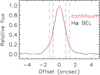 |
Fig. A.1. Brightness profile of Hα BEL and underlying continuum along the slit, extracted from the data with the best seeing condition (Feb 2020). We also show the slit width of 1.5″, 1.8″, and 2.5″ with dashed, dotted, and dash-dotted line, respectively. |
We demonstrate that the slight difference in the spatial distribution of continuum and Hα BEL does not cause a significant deviation of the measured EW of Hα using the following simulations. In the simulations, we assume that the EW of Hα remains constant (at the value observed in February 2020), and generate fake data that would be observed under different seeing conditions. We consider the effect of poorer seeing conditions by convolving the brightness profile of Hα BEL with Gaussian functions. We then measure the fractions of Hα BEL and continuum that fall into apertures. In Figure A.2, we show the ratio between the two under different seeing conditions for a slit width of 1.5″, 1.8″, and 2.5″, respectively. The ratios are normalized to the value measured in February 2020. This normalized ratio represents the deviation of the measured EW of Hα caused by changes in different seeing conditions and slit widths. The simulations show that the deviation is at most at a level of 7% for the seeing between 1.5″ and 3.3″, and the slit width between 1.5″ and 2.5″. We note that for the other four spectroscopic observations with poorer seeing conditions, the deviation is expected to be smaller. As the observed variations in the EW of Hα have a much larger amplitude than this value (up to 33%), we conclude that the Hα variability is intrinsic and cannot be explained by the variations in either seeing or slit width.
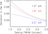 |
Fig. A.2. Deviation of measured Hα EW caused by the change in the seeing conditions using simulations, for slit widths of 1.5″ (black), 1.8″ (red), and 2.5″ (blue), respectively. |
Appendix B: UV-to-optical SED fittings
We fitted a blackbody model ( ) to the host-subtracted, extinction-corrected photometric data from the Swift UVOT observations during the period of optical outburst to put constraints on the luminosity, temperature, and radius evolution of UV and optical emission. Uncertainties on the above parameters were derived using Monte Carlo simulations, in which the observed fluxes were randomly perturbed with amplitude by assuming Gaussian noise according to the photometric errors. This procedure was repeated 1000 times. The error bars on each parameter were then derived from the 16th and 84th percentiles of the distribution of the corresponding values obtained in the simulations. The UV to optical SED for different epochs, with its best-fitting blackbody model, are shown in Figure B.1. Using the best-fit temperature and rest-frame monochromatic UV luminosity at each epoch, we estimated the blackbody radius from
 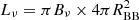 and took blackbody luminosity from
  as the integrated luminosity of UV and optical emission. The evolution of blackbody luminosity, temperature, and radius are presented in the Figure B.2.
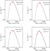 |
Fig. B.1. UV to optical SED obtained from the Swift UVOT observations during the period of the outburst, with the best-fit blackbody model for each epoch. |
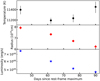 |
Fig. B.2. Evolution of UV/optical emission of CSS1029 at different epochs. From the top to the bottom panel, we show the evolution of blackbody luminosity, temperature, and radius, respectively, which are derived from blackbody fittings to the Swift UVOT data. |
All Tables
X-ray count rates, fluxes, and optical magnitudes for CSS1029 observed by Swift.
All Figures
|
Fig. 1. X-ray light curves observed at different epochs. Left panel: the evolution of the host-subtracted optical luminosity at the V-band is also shown (gray points, in units of 1042erg s−1). The solid line shows the best exponential fit, while the dotted line is the fit with the canonical t−5/3 decay law. The two best-fit lines are scaled down by a factor of 100 to match the X-ray light curve. |
| In the text | |
|
Fig. 2. X-ray spectrum by stacking three observations in 2010 (black) and five observations in 2015 (blue). The dotted line shows the best-fitted model consisting of a power law and a blackbody component. We note that the spectral fittings were performed jointly to the 2010 and 2015 data based on this model. The corresponding data-to-model ratios are shown in the bottom panel. |
| In the text | |
|
Fig. 3. Left: UV-to-X-ray spectral index αox versus 2500 Å luminosity for CSS1029 (black, green and blue symbols). The solid line represents the fit to the X-ray-selected AGNs from Grupe et al. (2010). The NSy1s are shown as gray dots, while the broad-line Sy1s are shown as gray triangles. For comparison, we also plot the αox for four typical NSy1s with extreme X-ray variations. The αox were calculated in the same manner as CSS1029. For clarity, only the two data points representing observations between the high and low state are shown. The open star represents the data for the thermal TDE ASASSN-14li in the flare state (van Velzen et al. 2016). Right: optical to X-ray SED of CSS1029. For clarity, only the data for the highest and lowest state within each epoch are shown. The median SED from radio-quiet quasars (Elvis et al. 1994) is also shown for comparison (dotted line), for which the luminosity is scaled to that of UVW2 obtained in the high state in 2015. |
| In the text | |
|
Fig. 4. P200/DBSP spectrum observed in February 2018 (orange) and February 2020 (gray) and the YFOSC spectrum observed in April 2020 (green), January 2021 (red), and May 2021 (cyan) in comparison with the archival SDSS spectrum taken in 2002 (blue). Lower panel: a zoomed-in view of the starlight-subtracted and continuum-subtracted spectra in the Hβ and Hα regions, which are calibrated using the [O III] narrow-line flux. |
| In the text | |
|
Fig. 5. Illustration of the emission-line-profile fitting in the Hα+[N II] region observed at different epochs. |
| In the text | |
|
Fig. 6. Variation of Hα, Hβ, and the continuum luminosity at 5100 Å as a function of time. Both broad and intermediate emission line components are shown. The dashed vertical line indicates the time of peak luminosity of optical outburst observed on Feb 23 2010 (D11). |
| In the text | |
|
Fig. 7. Comparison between the variation in the Hα broad line (purple) and that in medium width component (red) and the observed g-band continuum light curve (black points, see also Fig. 8). The orange solid line represents the linear fit, suggesting that the g-band flux variability can be described by a constant with little evolution over time. The dashed line indicates the 3σ scatter of flux variability relative to its mean. For clarity, the Hα flux has been normalized to the mean g-band flux on the date of Feb 24 2018, the start of our follow-up spectroscopic observations (thick vertical lines). Bottom panel: ratios of the g-band fluxes to the best-fit mean. |
| In the text | |
|
Fig. 8. Multi-wavelength light curves showing the changes in continuum over the past 15 years for CSS1029. Upper panel: UV (magenta) and X-ray (red) light curves observed from Swift. Bottom panel: light curve in the optical V-band from the CRTS DR2 (light orange), g-band from the ZTF DR2 (dark orange), and in the MIR 3.4 μm (cyan) and 4.6 μm (light blue) from WISE. The green dashed line represents the time of optical peak in 2010, and the X-ray peak in 2015, respectively. The gray thick lines show the time of our DBSP spectroscopy observations, while the blue thick lines indicate the time of YFOSC spectroscopy observations. |
| In the text | |
|
Fig. 9. Temperature evolution of UV-optical emission of CSS1029 compared with that of SLSNe and type II SNe (Inserra et al. 2018). The blue curve shows the blackbody temperature measured from the photometric data corrected for the Galactic dust extinction (EB − V = 0.015), while the purple curve represents that corrected for both the Galactic and internal dust extinction (EB − V = 0.073). The latter is estimated from the Balmer decrement of narrow emission lines (Drake et al. 2011). The temperature evolution of CSS1029 appears similar to that of optical TDE ASASSN-14ae (gray points, Holoien et al. 2014), as well as the peculiar SLSN ASASSN-15lh (black curve, Dong et al. 2016). The latter has been suggested to be more consistent with a TDE based on recent observations (Leloudas et al. 2016). |
| In the text | |
|
Fig. 10. Host-subtracted V-band light curve of CSS1029 (filled circles), and the best model realizations from MOSFIT (red curves). The most relevant best-fit model parameters are listed in Table 4. |
| In the text | |
|
Fig. 11. Posterior distributions of model parameters from the fit to the V-band light curve of CSS1029 shown in Fig. 10. The contours (from inside to outside) indicate the 1σ and 2σ confidence intervals for two parameters of interest, respectively. |
| In the text | |
|
Fig. 12. Host-subtracted WISE W2 (4.6 μm) magnitude for CSS1029 during outburst. For comparison, we also plot the evolution of the peak MIR luminosity of the TDE F01004-2237 (Dou et al. 2017) and PS16dtm (Blanchard et al. 2017), SLSNe (Jiang et al. 2019a), and the supernovae with an excess of MIR emission, i.e., Type Iax SN 2014dt (Fox et al. 2016). |
| In the text | |
|
Fig. A.1. Brightness profile of Hα BEL and underlying continuum along the slit, extracted from the data with the best seeing condition (Feb 2020). We also show the slit width of 1.5″, 1.8″, and 2.5″ with dashed, dotted, and dash-dotted line, respectively. |
| In the text | |
|
Fig. A.2. Deviation of measured Hα EW caused by the change in the seeing conditions using simulations, for slit widths of 1.5″ (black), 1.8″ (red), and 2.5″ (blue), respectively. |
| In the text | |
|
Fig. B.1. UV to optical SED obtained from the Swift UVOT observations during the period of the outburst, with the best-fit blackbody model for each epoch. |
| In the text | |
|
Fig. B.2. Evolution of UV/optical emission of CSS1029 at different epochs. From the top to the bottom panel, we show the evolution of blackbody luminosity, temperature, and radius, respectively, which are derived from blackbody fittings to the Swift UVOT data. |
| In the text | |
Current usage metrics show cumulative count of Article Views (full-text article views including HTML views, PDF and ePub downloads, according to the available data) and Abstracts Views on Vision4Press platform.
Data correspond to usage on the plateform after 2015. The current usage metrics is available 48-96 hours after online publication and is updated daily on week days.
Initial download of the metrics may take a while.