| Issue |
A&A
Volume 660, April 2022
|
|
|---|---|---|
| Article Number | A88 | |
| Number of page(s) | 46 | |
| Section | Extragalactic astronomy | |
| DOI | https://doi.org/10.1051/0004-6361/202142243 | |
| Published online | 14 April 2022 | |
The chemical composition of globular clusters in the Local Group⋆
1
Department of Astrophysics/IMAPP, Radboud University, PO Box 9010 6500 GL Nijmegen, The Netherlands
e-mail: s.larsen@astro.ru.nl
2
Ruprecht-Karls-Universität, Grabengasse 1, 69117 Heidelberg, Germany
3
Max-Planck-Institute for Astronomy, Königstuhl 17, 69117 Heidelberg, Germany
4
Niels Bohr International Academy, Niels Bohr Institute, Blegdamsvej 17, 2100 Copenhagen Ø, Denmark
5
Centre for Astrophysics and Supercomputing, Swinburne University of Technology, Hawthorn, VIC 3122, Australia
6
Department of Physics & Astronomy, One Washington Square, San José State University, San Jose, CA 95192, USA
7
University of California Observatories, 1156 High Street, Santa Cruz, CA 95064, USA
8
Department of Physics and Astronomy, Michigan State University, East Lansing, MI 48824, USA
Received:
17
September
2021
Accepted:
23
November
2021
We present detailed chemical abundance measurements for 45 globular clusters (GCs) associated with galaxies in (and, in one case, beyond) the Local Group. The measurements are based on new high-resolution integrated-light spectra of GCs in the galaxies NGC 185, NGC 205, M 31, M 33, and NGC 2403, combined with reanalysis of previously published observations of GCs in the Fornax dSph, WLM, NGC 147, NGC 6822, and the Milky Way. The GCs cover the range −2.8 < [Fe/H] < −0.1 and we determined abundances for Fe, Na, Mg, Si, Ca, Sc, Ti, Cr, Mn, Ni, Cu, Zn, Zr, Ba, and Eu. Corrections for non local thermodynamic equilibrium effects are included for Na, Mg, Ca, Ti, Mn, Fe, Ni, and Ba, building on a recently developed procedure. For several of the galaxies, our measurements provide the first quantitative constraints on the detailed composition of their metal-poor stellar populations. Overall, the GCs in different galaxies exhibit remarkably uniform abundance patterns of the α, iron-peak, and neutron-capture elements, with a dispersion of less than 0.1 dex in [α/Fe] for the full sample. There is a hint that GCs in dwarf galaxies are slightly less α-enhanced (by ∼0.04 dex on average) than those in larger galaxies. One GC in M 33 (HM33-B) resembles the most metal-rich GCs in the Fornax dSph (Fornax 4) and NGC 6822 (SC7) by having α-element abundances closer to scaled-solar values, possibly hinting at an accretion origin. A principal components analysis shows that the α-element abundances strongly correlate with those of Na, Sc, Ni, and Zn. Several GCs with [Fe/H] < −1.5 are deficient in Mg compared to other α-elements. We find no GCs with strongly enhanced r-process abundances as reported for metal-poor stars in some ultra-faint dwarfs and the Magellanic Clouds. The similarity of the abundance patterns for metal-poor GCs in different environments points to similar early enrichment histories and only allow for minor variations in the initial mass function.
Key words: galaxies: star clusters: general / galaxies: abundances / galaxies: evolution / stars: abundances / techniques: spectroscopic
Full Table F.1 is only available at the CDS via anonymous ftp to cdsarc.u-strasbg.fr (130.79.128.5) or via http://cdsarc.u-strasbg.fr/viz-bin/cat/J/A+A/660/A88
© ESO 2022
1. Introduction
The relative weakness of ‘metallic’ lines in the integrated spectra of globular cluster (GCs), which in some cases implies metallicities of less than 1% of the solar value, was noted long ago (Mayall 1946; Morgan 1956; Kinman 1959). Combined with the realisation that the more metal-poor GCs tend to be less concentrated towards the Galactic plane, this was an early harbinger of the first quantitative scenarios for the formation of the Milky Way (Eggen et al. 1962; Searle & Zinn 1978). In modern theories of galaxy formation, which are closely linked to the Λ-cold-dark-matter cosmological paradigm, present-day galaxies comprise a combination of stars that formed ‘in situ’ within the main progenitor halo and an ‘ex situ’ component that was built up through a sequence of mergers and accretion events (Navarro & White 1994; Cooper et al. 2010; Genel et al. 2014; Schaye et al. 2015). Simulations indicate that the in situ component typically dominates in low-mass galaxies and in the central regions of relatively massive (Milky-Way-like) galaxies, while ex situ stars become increasingly dominant at larger radii, especially in massive galaxies (Pillepich et al. 2015; Cook et al. 2016; Davison et al. 2021).
Direct evidence of these galaxy assembly processes abounds, not only in the obvious form of on-going major mergers, but also through identification of disrupted Milky Way satellite galaxies such as Sagittarius, Gaia-Enceladus, and others via analysis of the kinematics and chemistry of stars and GCs (Ibata et al. 1994; Helmi et al. 2018; Belokurov et al. 2018; Bergemann et al. 2018; Forbes 2020; Kruijssen et al. 2020; Woody & Schlaufman 2021). The large number of substructures in the halo of M 31 likewise attest to an active accretion history (Ibata et al. 2014; McConnachie et al. 2018), again with a close correspondence between features traced by halo field stars and GCs (Mackey et al. 2019). The wealth of detailed phase-space information that is now available from the Gaia mission has helped paint a rich and detailed picture of the accretion history of the Milky Way (Malhan et al. 2018; Brown 2021), especially in combination with chemical abundance information from ground-based spectroscopic surveys (Mackereth et al. 2019; Cordoni et al. 2021; Buder et al. 2021). However, because each galaxy has its own unique hierarchical assembly history, it is essential to establish to what extent lessons learned from detailed studies of the Milky Way can be generalised to other galaxies.
The chemical abundance patterns of stellar populations in galaxies contain valuable information about the assembly- and star formation histories. The various chemical elements are produced on different time scales by different mechanisms, and their relative abundances are therefore sensitive to the time scales of chemical enrichment and the relative importance of the various nucleosynthetic mechanisms. The ratio of α-capture elements to iron is a well-known indicator of the relative contributions from core-collapse (Type II) supernovae (SNe) on short timescales and Type Ia SNe with longer-lived progenitors (Tinsley 1979; Matteucci & Greggio 1986). The elements beyond the iron peak are mostly produced by neutron-capture processes in asymptotic giant branch (AGB) stars (s-process), neutron star mergers, or various types of exotic SNe (r-process) (Burbidge et al. 1957; Kobayashi et al. 2020). Within these broad categories, individual elements do not vary strictly in lockstep, as most elements are not produced by just a single mechanism. Among the α-elements, O and Mg are, at least in the Milky Way, the purest tracers of Type II SN nucleosynthesis, whereas Si and especially Ca and Ti also have significant contributions from Type Ia SNe (Kobayashi et al. 2020). However, Mg abundances can also be modified by hot hydrogen burning in AGB stars or massive stars, which may be responsible for the anomalous Mg abundances observed in some GC member stars (Gratton et al. 2012; Bastian & Lardo 2018). The iron-peak elements (e.g. Cr, Mn, Fe, and Ni) are thought to be produced mainly in Type Ia SNe, but they also have contributions from core collapse SNe (Kobayashi et al. 2020) and the production of Mn in particular is sensitive to SN Ia explosion physics and progenitor properties (McWilliam et al. 2003; Kirby et al. 2019; Eitner et al. 2020; Sanders et al. 2021).
In metal-poor Milky Way halo stars and GCs, the abundances of the α-elements are typically enhanced by about a factor of two compared to scaled-solar composition (Cohen 1978; Pilachowski et al. 1980; Sneden et al. 1979; Luck & Bond 1981). Similarly α-enhanced abundance patterns have been found for GCs and stars in the inner part of the M 31 halo (Beasley et al. 2005; Colucci et al. 2014; Sakari et al. 2016; Escala et al. 2019, 2020). In accordance with the above discussion, this suggests enrichment on time scales that were short relative to the delay before significant Type Ia SN enrichment set in (McWilliam 1997; Gilmore & Wyse 1998). However, the full picture is now known to be much more complex. At intermediate metallicities (−1.7 ≲ [Fe/H] ≲ −0.5), stars in the Milky Way halo display at least two distinct sequences in the [α/Fe] vs. [Fe/H] plane, of which the α-rich sequence is thought to be associated with the in situ component, while the less α-enhanced stars appear to be linked to the Gaia-Enceladus accretion event. The latter stars are also characterised by an enhancement of r-process elements relative to the α-elements (Nissen & Schuster 2010; Helmi et al. 2018; Matsuno et al. 2021a,b). The abundance patterns of the Gaia-Enceladus stars are reminiscent of those observed in nearby extant dwarf galaxies and likely reflect differences in the star formation histories relative to the more α-enhanced Galactic halo stars, with chemical enrichment proceeding at a slower pace in the dwarf galaxies (Shetrone et al. 2001; Venn et al. 2004; Tolstoy et al. 2009; McWilliam et al. 2013; Lemasle et al. 2014). The [α/Fe] patterns of stars in the outer parts of the M 31 halo (beyond ∼40 kpc) also tend to resemble those of stars in M 31 dwarf satellites more closely than stars nearer the centre (Gilbert et al. 2020), again indicative of a link between the dwarf satellites and the outer halo. These examples illustrate the role that chemical abundances can play in tracing hierarchical assembly histories of galaxies.
Detailed chemical abundance analysis of individual stars associated with old stellar populations is only feasible in the Milky Way and its nearest neighbouring galaxies with current astronomical facilities. The integrated light of entire galaxies can be observed to much greater distances, and spectroscopy of early-type galaxies has shown that they are typically dominated by relatively metal-rich, old stellar populations with increasingly enhanced α-element abundances for higher masses and velocity dispersions (Worthey et al. 1992; Kuntschner 2000; Trager et al. 2000; Thomas et al. 2005; Conroy et al. 2014; Kriek et al. 2019; Parikh et al. 2019). However, disentangling the mix of stellar populations with different ages and compositions that contribute to the integrated light is challenging, although some constraints on star formation histories and age-metallicity relations can be obtained from spectral inversion techniques (Peterken et al. 2020; Greener et al. 2021). GCs occupy an intermediate step between detailed studies of individual stars in nearby galaxies and the integrated light of more distant galaxies. They tend to be preferentially associated with the metal-poor, old components of galaxies, which usually contribute only a minor fraction of the integrated light, and they are therefore particularly useful tracers of these components. Apart from the Milky Way, association of GCs with substructure has been demonstrated in external galaxies such as M 31 (Mackey et al. 2019) and M 87 (Romanowsky et al. 2012).
Measurements of spectroscopic line indices on medium-resolution spectra of GCs is a well established technique for determining their ages and metallicities, and even obtaining some information about detailed abundances such as [α/Fe] ratios and nitrogen-enrichment (Brodie & Strader 2006; Schiavon et al. 2013). Based on such analyses, GCs around other galaxies tend to have similar old ages (∼10 Gyr) and α-enhanced composition to their Galactic counterparts (Larsen et al. 2002a; Beasley et al. 2008; Puzia et al. 2005; Strader et al. 2005; Cenarro et al. 2007). However, it is not yet entirely clear just how similar the abundances of GCs in different environments are. For GCs in the Local Group dwarf galaxies NGC 147, NGC 185, and NGC 205, Sharina et al. (2006) found α-element abundances consistent with scaled-solar values, and Puzia et al. (2006) found strongly α-enhanced ([α/Fe]> + 0.5) abundances for relatively metal-rich ([Fe/H] > −1) GCs in a sample of early-type galaxies. In contrast, Woodley et al. (2010) found GCs in the nearest giant elliptical, NGC 5128, to be only moderately α-enhanced with on average [α/Fe]= + 0.14, whereas [α/Fe] values for NGC 5128 GCs more similar to, or even slightly higher than those in Milky Way GCs, have been reported from detailed modelling of integrated-light spectra (Colucci et al. 2013; Hernandez et al. 2018). Differences between the abundance patterns in different types of galaxies could have important consequences for constraining their early chemical evolution, and could provide a basis for identification of different progenitor systems via ‘chemical tagging’ (Freeman & Bland-Hawthorn 2002; Sakari et al. 2014, 2015; Horta et al. 2020; Minelli et al. 2021).
Over the past decade, techniques to measure chemical abundances of individual elements from detailed modelling of integrated-light spectra, either from analysis of individual lines or from spectral fitting, have matured and have been applied to GCs in several studies. McWilliam & Bernstein (2008, hereafter MB2008) showed that abundances consistent with those measured for individual stars could be obtained from an integrated-light spectrum of the Galactic GC NGC 104 (47 Tuc). This type of analysis has since been further developed, tested, and applied in several studies (Colucci et al. 2009, 2017; Larsen et al. 2012, 2014, 2017; Sakari et al. 2013, 2015, 2016; Conroy et al. 2018; Rennó et al. 2020), and the abundances determined from integrated light generally agree with those obtained from individual stars within ∼0.1 dex. So far, these integrated-light studies have mostly adopted the standard simplifying assumptions of 1D, static model atmospheres and local thermodynamic equilibrium (LTE) in the analysis. Corrections for non-LTE (NLTE) effects are now becoming increasingly commonplace in abundance analyses of individual stars, and can in some cases lead to substantial differences. For example, Bergemann et al. (2017a,b) showed that the detailed [Mg/Fe] ratios in the low-α Galactic stars are sensitive to 3D and NLTE effects, although a distinction between Mg-rich and Mg-poor stars remains also in ⟨3D⟩ NLTE analysis (Bergemann et al. 2017b). Application of NLTE corrections to integrated-light measurements is complicated by the fact that the corrections vary depending on the physical parameters (effective temperature Teff, surface gravity log g, composition) of stars in different parts of the Hertzsprung–Russell diagram (HRD). NLTE corrections for integrated-light spectra were computed by Eitner et al. (2019) for Mg, Mn, and Ba, and were applied to observations of GCs by Eitner et al. (2020). Especially for Mn, the application of NLTE corrections significantly modified the results, largely eliminating the trend of decreasing [Mn/Fe] towards low metallicities seen in LTE analysis. As a consequence, the preferred model for Galactic chemical evolution changed from one in which Mn is produced in Type Ia SNe with sub-Chandrasekhar mass progenitors to one in which the progenitors have masses near the Chandrasekhar mass. Hence there is a clear need to further develop techniques for applying NLTE corrections to integrated-light abundance measurements.
In this paper we present a homogeneous analysis of integrated-light, high-resolution spectra of 45 GCs, mostly associated with Local Group galaxies but also including a cluster in the Sc-type galaxy NGC 2403. The galaxies span a range of morphological types, including all three Local Group spirals as well as several dwarf spheroidal and irregular galaxies. From detailed modelling of the GC spectra we measure the abundances of a large number of elements, including light- and α-elements (Na, Mg, Si, Ca, and Ti), iron-group elements (Sc, Cr, Mn, and Ni), and heavy elements (Cu, Zn, Zr, Ba, and Eu). A major update compared to previous papers is the inclusion of NLTE corrections for several elements, building on the work of Eitner et al. (2019, 2020). For the dwarf galaxies, our sample includes most of the old Local Group GCs that are bright enough for integrated-light spectra of sufficient signal-to-noise ratio (S/N, preferably better than about 100 per Å) to be obtained in a few hours of integration time, which translates to a magnitude limit of about V = 18. For the larger galaxies, in particular the Milky Way and M 31 with their rich GC systems, our sample only includes a small subset of the total GC populations. Nevertheless, the current sample is large enough that we can gain some insight into the degree of similarity between the chemical abundance patterns of GCs in different galaxies. As outlined above, this work is complementary to studies of field stars, as the GCs tend to preferentially trace the more metal-poor populations and their brightness makes it possible to constrain individual element abundances in more detail. In addition to this primary aim of comparing GCs within the Local Group, it is our hope that the data presented here will also serve as a useful reference for comparison with future work beyond the Local Group.
2. Data
The observations are summarised in Table A.1. Northern targets were observed with the HIRES spectrograph (Vogt et al. 1994) on the Keck I telescope and for the southern targets we used UVES (Dekker et al. 2000) on the ESO Very Large Telescope. In some cases, abundance analyses based on these observations have been published previously, with references that also provide more information about the reduction of these datasets given in the table. However, many aspects of our analysis technique have been updated (see below) and we here present a full reanalysis of all datasets. As such, the analysis in this paper supersedes the previous work, although the differences with respect to previous results are generally relatively minor (Sect. 4.1).
The July 2015 UVES observations of Milky Way GCs presented in Larsen et al. (2017, hereafter L2017) were combined with new observations of the same GCs obtained in August 2019. The July 2015 observations were obtained with the UVES red arm and the standard Cross Disperser #3, centred at 520 nm, while the August 2019 observations used the DIC2 dichroic and the CD#2 and CD#4 cross-dispersers in the blue and red arm, respectively. Together the two epochs cover the full spectral range 3300 Å−9500 Å at a spectral resolving power of ℛ ≡ λ/Δλ ∼ 40 000, where Δλ is the full width at half maximum of a resolution element. For both epochs of UVES observations the integrated light was sampled using a drift-scan technique whereby the UVES slit was scanned multiple times across the half-light diameter of each GC. In most cases, the same scanning patterns and exposure times were used for the two epochs. The August 2019 data were reduced in the same way as the July 2015 data, using the UVES pipeline running within the ESOREX environment to extract the calibrated 2D spectra. Separate sky exposures, bracketing the science exposures, were used to determine the sky level, which was then subtracted from the science exposures. Finally, the 2D spectra were collapsed to 1D spectra which were used in the analysis. For further details we refer to L2017. The same drift-scan technique was used for the integrated-light spectra of the GCs in the Fornax dSph, for which more details are given in Larsen et al. (2012).
Owing to their larger distances, the remaining GCs are sufficiently compact that their integrated light could be well sampled without having to rely on the relatively complex slit scanning procedure. The WLM GC was observed with UVES in a single setting (Larsen et al. 2014), while the rest of the data were obtained with HIRES. Most of the M 31 GC spectra come from two archival datasets, U017Hr (Oct. 1−3, 2007, P.I. G. Smith) and U118Hb (Oct. 18−19, 2007, P.I. K. Gregg), and four of the M 33 GC spectra are older data (Larsen et al. 2002b). Observations from the programme U017Hr were previously included in the study of mass-to-light ratios for M 31 GCs by Strader et al. (2009). The remaining HIRES data were obtained for this project as part of dedicated observing programmes.
Most of the HIRES observations were obtained after the instrument upgrade in 2004 (Butler et al. 2017). Apart from small gaps between the three detectors, the spectral coverage is continuous for wavelengths up to about 6300 Å. Above this limit the ends of the echelle orders fall off the edges of the detectors, leading to gaps in the wavelength coverage. The four M 33 GC spectra from Oct. 1998 were taken prior to the instrument upgrade, when HIRES only had a single detector. For these observations the total spectral range is therefore smaller and the ends of echelle orders already start falling off the ends of the detectors at wavelengths longer than ∼4500 Å. The location of the echellogram on the HIRES detectors can be adjusted by tilting the echelle grating and cross disperser, and not all datasets used the same settings. The exact wavelength coverage and location of the gaps in spectral coverage therefore vary from one dataset to another. The HIRES observations were typically obtained with the C5 decker which has a  slit and provides a resolving power of ℛ = 37 000. The 1998 and 2007 observations used somewhat narrower slits of
  and
and  , respectively, with correspondingly higher spectral resolving powers (ℛ being approximately proportional to the inverse slit width).
The HIRES data were reduced with the MAKEE (MAuna Kea Echelle Extraction) package1 written by T. Barlow. MAKEE automatically performs all reduction steps, from bias subtraction and flat-fielding of the raw exposures, to tracing of the spectral orders, optimal extraction, wavelength calibration, and resampling of the spectra to a linear wavelength scale. The details of the MAKEE reduction, such as constraints on the spectral extraction and background determination regions, are defined in a configuration file, where in most cases we used the standard configuration file as provided with MAKEE. The individual spectra of a given GC typically had identical exposure times and similar S/N and combined spectra were obtained as a straight (unweighted) sum of the extracted and calibrated 1D spectra of each GC. In the few cases that involved exposures of unequal duration, a more elaborate weighting scheme might in principle have produced combined spectra of slightly higher S/N. However, in practice the gain would be small: in the extreme case of read-noise limited data for which one exposure is many times longer than the other, the difference in S/N between an error-weighted average of the two exposures and a straight sum would amount to a factor of  , and for the typical exposures used here the difference is less than ∼5%. More details about the reduction of the HIRES spectra can be found in Larsen et al. (2018a).
For each combined GC spectrum, the S/N per Å, averaged over a 50 Å interval near 5000 Å, is listed in Table A.1. The S/N was estimated from the dispersion of the individual combined pixels at each wavelength sampling point. Because the linearisation of the wavelength scale involves interpolation between neighbouring pixel values, the dispersion of the individual values may underestimate the true uncertainties by up to a factor of  , and the final S/N values were therefore reduced by this factor. Nevertheless, the S/N values in Table A.1 should be considered approximate.
In Fig. 1 we plot the absolute visual magnitudes (MV) versus the iron abundances obtained from our analysis for the GCs. Distances and foreground extinctions mostly come from the references for the V magnitudes in Table A.1, except for M 31 where a distance modulus of (m − M)0 = 24.47 was assumed (Stanek & Garnavich 1998), and for M 33 where we adopted the distance modulus, (m − M)0 = 24.62, and reddening (E(B − V) = 0.19) from Gieren et al. (2013). The clusters span a range between [Fe/H] = −2.8 and −0.1, with the more metal-rich GCs preferentially being associated with the Milky Way and M 31 and the more metal-poor ones preferentially with the dwarf galaxies in our sample. We also note that the M 31 GCs in our sample are among the brightest in that galaxy, and are generally brighter than those associated with the dwarf galaxies.
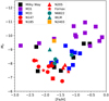 |
Fig. 1. Absolute visual magnitude (MV) as a function of metallicity for the observed GCs. Symbol colours and shapes identify the host galaxy as indicated in the legend. |
3. Analysis
The basic analysis framework remains similar to that described in several previous papers (Larsen et al. 2012, 2017, 2018a). Briefly stated, we proceed by computing simple stellar population (SSP) model spectra at high spectral resolving power while adjusting the abundances of individual elements until the best fits to the observed spectra are obtained. An outline of the main steps follows below (Sect. 3.1). Compared to previous analyses, some of the main updates for this work include the use of ATLAS12 model atmospheres with compositions that self-consistently match those derived from the spectra (Sect. 3.2), a redefinition of the spectral windows used to fit the abundances of some elements (Sect. 3.3), an extensive revision of the line list (Sect. 3.4), and a modified prescription for assigning microturbulence velocities to individual stars (Sect. 3.6). For the first time, we also include NLTE corrections for our integrated-light abundance measurements for several elements (Sect. 3.7).
3.1. General outline of the procedure
We assume that GCs can be modelled as SSPs, that is, as consisting of stars with a single age and chemical composition. This is clearly an oversimplification, given that a number of (especially light) elements are known to exhibit significant abundance spreads within GCs (Bastian & Lardo 2018; Gratton et al. 2019). However, attempting to constrain such abundance spreads from integrated-light measurements is beyond the scope of this work (but see Larsen et al. 2018b) and what we measure here is thus an average abundance for each element. Populations of stars with different abundances contribute to this average with weights that depend on the response of individual spectral features to the abundance variations (Larsen et al. 2017).
To compute an integrated-light model spectrum, we must first specify the distribution of stars in the HRD. In general, this information may come from a theoretical isochrone or from an empirical colour–magnitude diagram (CMD), or some combination of the two. In practice, the HRD is provided as a set of approximately 100 bins (‘HRD-boxes’), each representing a group of stars with specific physical parameters (effective temperature Teff, surface gravity log g, and radius R). The chemical composition is assumed to be the same for all HRD-boxes. Model atmospheres and synthetic spectra are then computed for each HRD-box and the synthesised surface fluxes are scaled by the surface areas of the stars to provide luminosities, which are finally co-added with weights corresponding to the numbers of stars associated with each HRD-box. The result is an integrated-light SSP model spectrum for the assumed chemical composition and HRD parameters, calculated at a spectral resolving power that is sufficiently high to sample the line profiles (typically ℛ = 500 000). The SSP model spectrum is then convolved with a Gaussian kernel to account for instrumental resolution and velocity broadening in the cluster, it is scaled to the (radial velocity corrected) observed spectrum using a spline or polynomial fitting function to match the continuum levels, and the χ2 is computed for the model–data difference. The input abundances are then adjusted and the procedure is repeated until the best fit is obtained. In principle, our implementation of this technique allows for any arbitrary number of element abundances to be fitted simultaneously, but in practice we usually fit for one element at a time using spectral windows tailored specifically to the features of interest for each element. Errors are estimated by varying the abundances until the χ2 value has increased by one, compared to the best-fit value.
The procedure is implemented as a Python 3 package that we have named ISPy3 (Integrated-light Spectroscopy with Python 3). The Python code is publically available via Github (Larsen 2020). The model atmosphere and spectral synthesis calculations are done via calls to external codes, with the currently supported options being either the Kurucz ATLAS9/ATLAS12 and SYNTHE codes (Kurucz 1970, 2005; Kurucz & Avrett 1981) or MARCS model atmospheres in combination with Turbospectrum (Gustafsson et al. 2008; Alvarez & Plez 1998; Plez 2012).
3.2. Model atmospheres
In previous papers we have relied mostly on the Linux versions of the ATLAS9 and SYNTHE codes (Sbordone et al. 2004) for the model atmospheres and spectral synthesis while employing spherically symmetric MARCS models and Turbospectrum (Alvarez & Plez 1998) for the modelling of the coolest giants. Each combination has pros and cons: the ATLAS9/ATLAS12 codes are publically available and can therefore be used to compute models for any desired combination of stellar parameters (Teff, log g, and chemical composition), but ATLAS models are limited to plane parallel geometry. The MARCS grid includes models with spherical geometry, but models must be interpolated for physical parameters not included in the pre-computed grid available from the MARCS website2.
The ATLAS models come in two flavours. In ATLAS9, the line opacity is modelled via pre-computed opacity distribution functions (ODFs) and models are thus restricted to the abundance patterns used when computing the ODFs. Recomputing the ODFs for different abundance patterns is a time consuming process and becomes impractical if models with many different abundance patterns are needed. The ATLAS12 code uses the opacity sampling technique to compute models for arbitrary abundance patterns, but at a much higher computational cost per individual model. It should be noted that, even in ATLAS9, the detailed abundance patterns specified when computing a model do affect the continuum opacity, especially for elements that are important electron donors (such as Na, Mg, Si, and Ca) and therefore have a significant effect on the H− opacity and the resulting atmospheric structure. If the spectral synthesis is subsequently done for abundance patterns that do not match those used when computing the atmosphere models, inconsistencies can arise.
For the analysis presented here we used ATLAS12 for stars hotter than Teff = 4000 K to compute model atmospheres with abundance patterns matching those determined from the spectroscopic analysis. As the abundance patterns are not known a priori, this required an iterative approach whereby we started with an initial guess for the input abundances (for the GCs, typically a 0.3 dex enhancement of the α-elements relative to scaled-solar composition), then fitted for the abundances, and recomputed the model atmospheres. Since the spectral synthesis is, after all, only moderately sensitive to the exact abundances assumed when computing the model atmospheres, this procedure usually required only 2 or 3 iterations. For the cooler stars, both dwarfs and giants, we continue to rely on MARCS and Turbospectrum. The motivation for this is two-fold: at low surface gravities, departures from plane-parallel geometry become increasingly important, and at high surface gravities the ATLAS models with low temperatures occasionally fail to converge properly, particularly at low metallicities. ISPy3 uses the programme interpol_modeles (Masseron 2006) to interpolate between models for the Teff, log g, and [Fe/H] values included in the MARCS grid. We used the ‘standard composition’ grid for which the models are computed for an α-element enhancement of [α/Fe]= + 0.4 at metallicities [Fe/H] ≤ −1, gradually decreasing to scaled-solar composition at [Fe/H] = 0. For the spectral synthesis we used the same atomic and molecular line lists for SYNTHE and Turbospectrum (see Sect. 3.4), except for TiO for which SYNTHE uses the line list by Schwenke (1998) while Turbospectrum uses the line list by Plez (1998).
3.3. Spectral windows
To aid us in updating the line list and (re-)defining the windows used for the spectral fitting, we used the Wallace et al. (2000) spectrum of Arcturus (spectral type K1.5 III; Keenan & McNeil 1989) and the 2005 version of the Kurucz et al. (1984) spectrum of the Sun. The Arcturus spectrum has a S/N of about 1000, sampled at 0.06 Å resolution near 5000 Å (corresponding to a S/N ∼ 13 000 per Å), while the solar spectrum has an even higher S/N of > 2000 per 0.05 Å sampling interval (Furenlid 1988). In both cases, this is far higher than the S/N of any of our GC spectra. Because this part of the analysis was done at an early stage of the project, we used ATLAS9 to compute a model atmosphere for each star, assuming an effective temperature of Teff = 4286 K, surface gravity log g = 1.66, and an initial metallicity [Fe/H] = −0.6 for Arcturus (Worley et al. 2009; Ramírez & Allende Prieto 2011) and Teff = 5777 K, log g = 4.44, and [Fe/H] = 0 for the Sun (Cox 2000). For each model atmosphere, we used the WIDTH9 code (Castelli 2005; Kurucz 2005) to calculate equivalent widths for all atomic lines in the most recent version of the line list at the Kurucz website3 (dated 8 Oct. 2017). Synthetic spectra were computed with SYNTHE.
For iron we defined 40 new spectral windows. These windows were defined primarily via a visual inspection of the Arcturus spectrum alongside the corresponding SYNTHE model spectrum, using the list of equivalent widths to label the stronger lines. In order to be useful for measuring iron abundances also at low metallicities, we made sure that each spectral window contained lines with a range of equivalent widths, also including relatively strong lines with equivalent widths ≳100 mÅ. At wavelengths < 4400 Å the spectra of late-type stars become strongly affected by CH molecular absorption bands and by increased line blending in general, and we therefore concentrated on the spectral range λ > 4400 Å. Together, our 40 iron windows cover about 45% of the wavelength range 4570 Å−6185 Å but include about 60% of the Fe lines stronger than 100 mÅ. We also defined ten new windows for Ca, 14 windows for Ti, and 18 windows for Cr that replace the broader windows used to fit for the abundances of these elements in previous papers. While the velocity broadening of GC spectra implies that all lines are affected by blending at some level, we made an effort to define these new windows in such a way that relatively clean lines were prioritised. A full listing of the window definitions can be found in Table B.1.
We added several chemical elements not measured in the previous analyses, in some cases taking advantage of the fact that many of the spectra used here extend well beyond the 6200 Å limit of older analyses. For Si, we included six windows in the range 5660 Å−7430 Å and for Ba we added the Ba II line at 6497 Å. When possible, we also included Zn, Zr, and Eu among the elements measured. Our Eu measurements are based on the Eu II lines at 4435 Å and at 6645 Å, but not all observed spectra include both lines. Some of our spectra include the [O I] line at 6300 Å but the line is very weak even in the spectra of metal-rich GCs like 47 Tuc and it is often contaminated by telluric O2 and H2O absorption and/or residuals from the corresponding [O I] night sky line. We therefore did not attempt to measure oxygen.
3.4. The line list
Previous papers based on the analysis technique used here employed the atomic line list of Castelli & Hubrig (2004, hereafter CH2004), with a few minor modifications, as input for the spectral synthesis. That line list is itself a modified version of an older version of the Kurucz line list (see CH2004 for details). However, it was clear from a comparison with high-resolution spectra of Arcturus and the Sun that not all lines are well reproduced in model spectra computed with the CH2004 list (Larsen et al. 2012). This is a common occurrence when using standard line lists to model observed spectra in detail, owing to the fact that atomic data remain uncertain for many transitions that are detectable even in the spectra of solar-type stars (Jofré et al. 2019). One (partial) solution is to derive ‘astrophysical’ oscillator strengths (log gf values) by requiring that the lines in a model spectrum match those in observations (Shetrone et al. 2015; Boeche & Grebel 2016; Laverick et al. 2019). Some limitations of this approach are that the line data are then tied to a chosen abundance scale, to the physics of underlying stellar atmosphere models, and to the details of the analysis method, such as inclusion (or not) of NLTE effects, and that blended lines can be difficult to treat. For this work we opted to critically evaluate the input line list, while still relying as much as possible on existing sources for the atomic data.
Having defined the spectral windows, we proceeded to adjust the input line list via a visual inspection of the fits to the solar and Arcturus spectra. We used the 8 Oct. 2017 Kurucz list of atomic transitions as a starting point, and whenever a poor match between the observed and synthetic spectra was found, the log gf value in the Kurucz list was compared with the values in the CH2004 and VALD (Piskunov et al. 1995; Kupka et al. 1999) lists to see if these gave a better fit. In a few cases, the NIST database (Kramida et al. 2013) was also consulted. While it was frequently possible to obtain clear improvements to the fits in this way, no single compilation of line data was found to be satisfactory for all lines. In some cases, the data in all three lists were found to be unsatisfactory, and we resorted to adjusting the log gf values by hand or removing lines altogether. In total, the log gf values for some 735 atomic lines were modified (counting lines with hyperfine structure only once), with the CH2004 values being preferred for 274 lines, the VALD values for 105 lines, and VALD and CH2004 listing identical (preferred) values for 84 lines. For most of the remaining 272 modified entries, the log gf values were manually adjusted. When updating the line data, an additional criterion was to minimise the scatter between abundance determinations for a given element in different windows. The median absolute change in the log gf values was 0.46 dex and for 15% of the lines the change was greater than 1 dex. About 4% of the modified lines were changed by more than 2 dex. The lines we have adjusted represent only a very small fraction of all lines in the Kurucz list, which contains more than 300 000 atomic transitions between 4200 Å and 6200 Å and another > 130 000 between 6200 Å and 7500 Å. However, most of these are far too weak to be detectable in our spectra. While many of the modified lines are not among those actually measured in a specific spectral window, they may still influence the fits through blending or by biasing the overall scaling of the continuum levels, and we therefore tried to get good fits for as many lines as possible.
The Kurucz line list includes hyperfine splitting for many species (Na I, Al I, Al II, K I, Sc I, Sc II, V I, Mn I, Mn II, Co I, Ni II, Cu I, Y I, Y II, Nb I, Nb II, Ba I, Ba II, La II, and Eu II). Since the relative strengths of the hyperfine components are specified in a separate column in the data file, it was straight forward to adjust the oscillator strengths for all components of a given line.
For the lines of Mg I, we mostly adopted NIST log gf values, while for lines of Si I, Ti I, and Fe I the values from the CH2004 list were frequently found to give the best results. The Mg I lines at 4351.906 Å and 4354.528 Å are affected by blending with CH molecular lines and are not generally used in our analysis, but we have verified that the results are not very sensitive to inclusion or not of these lines. For Ca I, the most consistent results were typically obtained when using the log gf values in the VALD database, which come mostly from Smith & Raggett (1981). However, for some Ca I lines we kept the log gf values in the Kurucz list, some of which date back to Wiese et al. (1969). Damping coefficients describing line broadening caused by elastic collisions between ions and hydrogen were adopted from Barklem et al. (2000) for some of the stronger lines (Mg Ib, many of the Ca I lines, and the Ba II lines). For a few lines, mostly from Sc II and Zr I, the wavelengths in the Kurucz line list were found to be off by small amounts (20−40 mÅ) and we adopted wavelengths from VALD or CH2004 to match the positions of these lines in the spectra of Arcturus and the Sun.
At first, the Zr I lines were found to be systematically too strong in the model spectra computed with SYNTHE. We were unable to attribute this to problems with the oscillator strengths, and found that models computed with Turbospectrum matched the Arcturus spectrum well for these lines. The difference was traced to different ionisation potentials for Zr I used in the two codes. In SYNTHE, an ionisation potential of 6.840 eV was hard-coded for this species (from Drawin & Felenbok 1965), whereas Turbospectrum instead uses a value of 6.634 eV which agrees with more recent determinations (Liu et al. 2019). We updated the Zr I ionisation potential and the partition function for Zr I in SYNTHE, using the same polynomial fitting functions as in Turbospectrum (Irwin 1981) for the partition function. With these modifications, the Zr I lines in the SYNTHE spectrum were found to match those computed with Turbospectrum. We also compared the ionisation potentials for other ions, and found any remaining differences between the values used in Turbospectrum and SYNTHE to be negligible.
In some cases it was not possible to get a good fit despite our best efforts – typically because a line was present in the observed spectra but not in the synthetic ones, or in cases where complex blends made it difficult or impossible to unambiguously determine the correct log gf values for the individual lines. In such cases, the affected spectral regions were marked and masked out in the analysis.
For molecular lines we mostly used the data available at the Kurucz website. This includes data for the following molecules: H2, NH, OH, NaH, MgH, AlH, SiH, CaH, TiH, CrH, FeH, C2, CN, CO, AlO, SiO, CaO, TiO, VO, and H2O. For the CN line list, an error was detected in the conversion of the f-values in the original data (Brooke et al. 2014) to the log gf values in the line list at the Kurucz website. We therefore updated the CN line data accordingly. For CH we used the line list from Masseron et al. (2014), which is available from the website of B. Plez4. Nevertheless, these updates are of relatively minor consequence for this work, since the CN and CH lines mostly affect the spectra at wavelengths < 4400 Å. In principle, the CN and CH features in the wavelength range 4100 Å–4400 Å can be used to constrain the abundances of C and N, although the N abundances are better constrained by the stronger CN band near 3800 Å–3900 Å, especially at lower metallicities (Cohen et al. 2002; Graves & Schiavon 2008; Lardo et al. 2012; Schiavon et al. 2013; Martocchia et al. 2021). However, the interpretation of C and N abundances in integrated-light spectra is complicated by stellar evolutionary effects (mixing) along the red giant branch (RGB) (Gratton et al. 2000; Martell et al. 2008), and we do not here quote abundances of these elements.
To illustrate the procedure by which the line list was customised, Fig. 2 shows model fits to a small region of the spectra of Arcturus and the Sun. The fits are shown for the Kurucz line list and the CH2004 list, as well as for our final adopted version of the Kurucz list. These fits are fairly typical and reveal significant differences between the observed and synthetic spectra for both the CH2004 and Kurucz lists. Within this region, spanning only a few Å, we modified the oscillator strengths for several lines, of which we discuss a few representative examples. The most striking mismatch is for the Ni I line at 4971.591 Å, which is much too strong when using the data from the Kurucz list. For this line the Kurucz list has log gf = −0.753, which is the same value listed in the VALD database. In the CH2004 list the line has log gf = −1.566, but this still makes the line much too strong in the synthetic spectra. This line was removed altogether from the line list. The neighbouring Ni I line at 4971.34 Å is well matched when using the Kurucz list, but much too weak in the spectrum computed with the CH2004 list. A more typical example is the Ni I line at 4967.524 Å, which is too weak when using the Kurucz list. For this line, the Kurucz list has a lower log gf value (−1.989) than VALD and Castelli (log gf = −1.570), and using the latter value clearly gives a better fit. Sorting out the blend between 4968 Å and 4969 Å was more complicated. The Fe I line at 4968.276 Å was found to be too strong in both the Kurucz and VALD lists (log gf = −2.043), but using the much lower log gf value from CH2004 (log gf = −3.653) gave a satisfactory fit. The Fe I line at 4968.392 Å remained too strong in all three line lists, and the log gf value was manually adjusted downward from the value in the Kurucz list (−1.409) to log gf = −1.8. For the Ti I line at 4968.567 Å, the Castelli value (log gf = −0.44) was used instead of the value common to the Kurucz and VALD lists (log gf = −0.64). Nevertheless, the fit remains somewhat unsatisfactory for this rather complex blend, and situations like this could not always be completely resolved. The weak feature near 4971.0 Å is a blend that includes the Nd II line marked in the figure (with an equivalent width of about 10 mÅ in the Arcturus spectrum), as well as various other features (Co I, V I). The CH2004 data appear to give a better fit to the Arcturus spectrum, but overpredict the strength of the lines in the solar spectrum, and in this case we did not modify the Kurucz data.
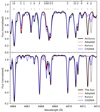 |
Fig. 2. Fits to the spectra of Arcturus (top) and the Sun (bottom). Model spectra were computed using the standard Kurucz line list, the Castelli & Hubrig (2004) list, and our adopted version of the Kurucz list, as indicated in the legend. |
The final line list was converted from the format used by SYNTHE to that used by Turbospectrum to ensure consistent modelling with the two codes. This was mostly a straight forward procedure, amounting mainly to unit conversions and some reformatting. We left out more than twice ionised species, which are not supported by Turbospectrum and are, in any case, of no relevance in the cool stars modelled with Turbospectrum. We also excluded a few transitions with excitation potentials greater than 100 eV which caused problems for the Turbospectrum format and would introduce no observable lines in any spectra of relevance here.
3.5. Single star validation: The Sun and Arcturus
As a first verification of the analysis procedure, abundances were determined for the Sun and Arcturus and compared with literature results for these well-studied stars. We discuss each in turn below.
3.5.1. The Sun
The solar spectrum was analysed using an ATLAS12 atmosphere and SYNTHE. One remaining parameter to fix is the microturbulence velocity, vt, assumed for the spectral synthesis (e.g. Jefferies 1968). For solar-type stars, typical microturbulence velocities used for classical abundance analysis are vt ≃ 1 km s−1. Recent examples include vt = 0.85 km s−1 (Valenti & Fischer 2005; Yong et al. 2005; Brewer et al. 2015), 0.93 km s−1 (Fulbright et al. 2006), 0.75 km s−1 (Pavlenko et al. 2012), and 1.10 km s−1 (Laverick et al. 2019). From a comparison with 3D models, Dutra-Ferreira et al. (2016) found microturbulence velocities of ∼1 km s−1 for dwarf stars with their Eq. (2) yielding vt = 0.97 km s−1 for the solar Teff and log g. We analysed the solar spectrum using two values of the microturbulence, vt = 0.85 km s−1 and vt = 1.0 km s−1.
Our average abundance measurements for the Sun are listed in Table 1 together with the standard solar compositions of Grevesse & Sauval (1998, hereafter GS1998) and Asplund et al. (2009, A2009). The abundances are normalised to a logarithmic hydrogen abundance of 12 + log ϵ(H) = 12. The numbers in parentheses are the rms dispersions of the individual measurements for each element and N are the numbers of measurements (spectral windows) per element. We list the NLTE abundances for elements for which these are available and LTE abundances otherwise. Due to the extremely high S/N of the Kurucz solar spectrum, the formal errors on the fits are negligibly small and the scatter between the abundance measurements in different spectral windows for a given element is almost entirely due to systematics. We therefore computed the abundances in the table as a straight average of the individual measurements. For most elements, the scatter is less than about 0.1 dex, although a somewhat larger scatter is found for nickel. As expected, using the larger vt value reduces the effect of line saturation, which in turn leads to a slight decrease (0.02−0.04 dex) in the abundances of most elements.
Solar analysis.
We briefly comment on a few individual elements. Iron is often used as a proxy for metallicity, and when presenting our results for the GCs we generally follow the usual convention and give the abundances of other elements as [X/Fe]. GS1998 and A2009 both list the same iron abundance of 12 + log ϵ(Fe) = 7.50 for the Sun with uncertainties of 0.04−0.05 dex. Our NLTE measurement of the solar iron abundance for vt = 0.85 km s−1 matches this value exactly. For vt = 1.0 km s−1 we find a slightly lower value of 12 + log ϵ(Fe) = 7.48, which is still well within the uncertainties on the reference values. For two elements, Zr and Eu, the differences with respect to GS1998 and A2009 are relatively large (0.2−0.3 dex), although NLTE corrections are not included for these elements. However, our choices of spectral features are not optimised for measuring these elements in the solar spectrum. The blue Eu II line at 4435.6 Å, with an equivalent width of about 25 mÅ, is blended with a much stronger Ca I line (equivalent width ∼170 mÅ) at 4435.7 Å, and the derived Eu abundance is therefore sensitive to uncertainties in the Ca abundance and to the details of the spectral synthesis, such as the inclusion of velocity-dependent van der Waals broadening constants for the Ca line (Anstee & O’Mara 1995). From varying the Ca abundance, we found that a decrease of just 0.06 dex in log ϵ(Ca) would increase log ϵ(Eu) to match the reference values. The red Eu II line, centred at 6645.10 Å, is quite weak in the solar spectrum (4 mÅ) and is blended with an Al I line at 6645.14 Å that has an equivalent width of 13 mÅ. We could not get a reliable estimate of the Eu abundance from this line for the Sun. In cool giants the relative strengths of the lines in these blends change in favour of the Eu lines, but it is nevertheless clear that the measurements of Eu must be considered somewhat uncertain.
The Zr I lines in the window 6124 Å–6147 Å are also very weak in the solar spectrum (the equivalent widths are < 3 mÅ), and some are blended with stronger lines. In particular, the Zr I line at 6124.9 Å is blended with a much stronger Si I line at 6125.0 Å. There are other lines that would be more suitable for measuring Zr in the solar spectrum, but these are mostly located in the blue (λ < 4400 nm) and are less useful for analysis of GC spectra due to blending with molecular and atomic features.
Excluding Eu and Zr, our measurements agree well with the reference scales overall. For the abundances that include NLTE corrections, the mean offsets with respect to GS1998 are ⟨log10ϵ − log10ϵGS98⟩= − 0.01 dex (for vt = 0.85 km s−1) and −0.04 dex (vt = 1.0 km s−1). Comparing with A2009, the offsets are instead ⟨log10ϵ − log10ϵA09⟩= + 0.00 dex (for vt = 0.85 km s−1) and −0.02 dex (vt = 1.0 km s−1). If we additionally include the elements measured in LTE, the mean offsets are −0.02 dex and −0.05 dex for GS1998 for the two vt values, respectively, and 0.00 dex and −0.03 dex for A2009. There is thus no strong preference for either vt value, but we adopt vt = 0.85 km s−1 as the preferred value here as it reproduces the iron reference abundances more closely. We note, however, that the vt = 1.0 km s−1 measurements tend to give a slightly smaller rms scatter for most elements.
At any rate, it is unsurprising that our analysis does not exactly reproduce either of the two standard abundance scales for every element. Our analysis technique is not optimised for the solar spectrum and the A2009 abundance scale, in particular, is based on a much more sophisticated analysis that employs 3D NLTE hydrodynamical model calculations for many elements.
In the remainder of this paper, we quote abundances relative to the scale of GS1998 for consistency with previous papers based on our technique. Readers who prefer to convert our measurements to the scale of A2009, or to adopt a differential comparison with respect to our solar abundance measurements, can do so using the information in Table 1. The caveat should, however, be kept in mind that the spectral windows typically have different weights in the analysis of the GC spectra (depending on the uncertainty on each measurement; Sect. 3.8) compared to the uniform weights used for our solar analysis in Table 1.
3.5.2. Arcturus
As an RGB star, the spectrum of Arcturus resembles that of a GC much more closely than does the solar spectrum. As such, the Arcturus spectrum provides a better test of the suitability of our line list (and of our analysis technique in general) for analysis of GC spectra. The drawback is that the composition of Arcturus is not as well established as that of the Sun. Nevertheless, the distance and diameter of Arcturus are well constrained by parallax and interferometric measurements, and consequently other physical parameters are also well determined. The effective temperature and surface gravity adopted here (Sect. 3.3) are very similar to those used in other studies (e.g. Fulbright et al. 2006; Worley et al. 2009). For the microturbulence, values quoted in the literature range from vt = 1.2 km s−1 (from analysis of infrared lines, Kondo et al. 2019) to 1.8−1.9 km s−1 (Van der Swaelmen et al. 2013, vdS2013), with other studies finding intermediate values of 1.50 km s−1 (Worley et al. 2009, W2009), 1.56 km s−1 (Yong et al. 2005, Y2005), 1.67 km s−1 (Fulbright et al. 2006), and vt = 1.74 km s−1 (Ramírez & Allende Prieto 2011, RA2011).
In Table 2 we list our abundance measurements for Arcturus obtained with ATLAS12/SYNTHE for two values of the microturbulence, vt = 1.50 km s−1 and 1.74 km s−1. To assess the sensitivity of the measurements to the choice of model atmospheres and spectral synthesis codes, we also include results obtained with ATLAS9/SYNTHE (A9/S), with ATLAS12/Turbospectrum (A12/T), and with spherical MARCS models and Turbospectrum (M/T). These latter results are given for a single value of the microturbulence, vt = 1.50 km s−1. We also include abundance measurements from previous studies for comparison. The literature results are listed as given in the respective papers with no attempt to homogenise the reference abundance scales, oscillator strengths, line lists, or other parameters that can cause systematic offsets in the results. We comment on some of these issues below. To facilitate easier comparison with the literature results (none of which accounts for NLTE effects) our measurements in the table are also given as LTE values. The comparison of our results for different details of the analysis would be unaffected by the inclusion of NLTE corrections. However, we give the NLTE corrections, ΔNLTE, for elements where these have been determined (Sect. 3.7).
Arcturus LTE analysis.
The choices of model atmospheres and spectral synthesis codes have a relatively minor effect on the results. The iron abundances obtained with SYNTHE (for vt = 1.50 km s−1) and Turbospectrum differ by only 0.011 dex when using the same (ATLAS12) model atmospheres, and replacing the ATLAS12 atmospheres with ATLAS9 models leads to an even smaller difference (0.002 dex). The iron abundances fall, in these cases ([Fe/H] = −0.58 to [Fe/H] = −0.59), well within the range found in the literature. When using MARCS atmospheres instead of ATLAS12 (both in combination with Turbospectrum), the iron abundance decreases by 0.03 dex but remains within the literature range. Using vt = 1.74 km s−1 for the microturbulence leads to a decrease of about 0.1 dex in [Fe/H]. This lower iron abundance ([Fe/H] = −0.68) appears to be somewhat disfavoured by comparison with the literature values, although vdS2013 found iron abundances between [Fe/H] = −0.58 and −0.71 depending on the amount of noise they added to the Arcturus spectrum. The values with which we compare in Table 2 are for their ‘∞S/N’ analysis, which, for most elements, yields fairly similar results to our analysis with vt = 1.74 km s−1. In this sense, the relatively high [Fe/H] = −0.52 from RA2011, who used the same high vt value, is more discrepant.
For most elemental abundance ratios, the analyses based on SYNTHE or Turbospectrum in combination with ATLAS12 model atmospheres yield very similar results that agree well with the literature values. For Si and Ba, the analyses based on Turbospectrum yield somewhat higher abundances ratios (by 0.06 dex and 0.08 dex, respectively) than those based on SYNTHE. More typically the differences are 0.01−0.02 dex. Again, the results are relatively insensitive to the choice of MARCS versus ATLAS12 models, while the choice of microturbulence can lead to differences of ∼0.05 dex in the derived abundance ratios.
Of the literature results listed in Table 2, two are differential analyses with respect to the Sun (Y2005; RA2011). The study by W2009 is an LTE analysis with abundances given relative to the solar abundance scale of Lodders (2003, L2003), which differs only slightly from the GS1998 scale used in our analysis for most elements. The largest differences between the two scales are found for Ti (12 + log ϵ(Ti) = 4.92 on the L2003 scale) and Sc (12 + log ϵ(Sc) = 3.07), that is, the solar abundances are 0.1 dex lower than on the GS1998 scale for both elements. This likely accounts for the offsets between our abundance determinations for these elements and those of W2009. The analysis of vdS2013 also assumes LTE and abundances are given relative to the GS1998 scale, as in the present work. The literature results are all based on the same high-resolution, high S/N spectrum of Arcturus that we are using here.
For Na, systematics at the level of 0.1 dex arise from two sources: first, the solar reference abundance according to A2009 is 0.09 dex lower than the GS1998 value, so that our [Na/Fe] values would increase by the same amount if given relative to the A2009 scale. Second, inclusion of NLTE corrections would decrease our [Na/Fe] value for Arcturus by 0.19 dex. Our analysis is most directly comparable with those of W2009 and vdS2013, compared with which studies our [Na/Fe] value for Arcturus is 0.05−0.09 dex higher. Our LTE analysis of the solar spectrum recovers the GS1998 Na abundance almost exactly (12 + log ϵ(Na) = 6.33) so that we may also reasonably compare our measurements for Arcturus on the GS1998 scale with the differential analyses by Y2005 and RA2011. Again, our values are slightly higher (0.04−0.08 dex). However, in LTE we also find a slightly lower iron abundance for the Sun, 12 + log ϵ(Fe) = 7.47 (for vt = 0.85 km s−1). An adjustment for the 0.03 dex difference relative to the GS1998 scale would lead to a corresponding increase in the differential [Fe/H] value for Arcturus, and therefore a decrease in the differential [Na/Fe] value by the same amount, which would bring our measurement of [Na/Fe] very close to that of Y2005, and within 0.05 dex of that of RA2011.
For Zr and Eu our measurements for Arcturus fall within the range quoted in the literature, although the literature values for [Zr/Fe] span a range of 0.3 dex. For Cu, the only other measurement is that of vdS2013, whose [Cu/Fe] ratio is about 0.26 dex lower than ours. The Cu abundances obtained from our measurements of the two Cu I lines (at 5106 Å and 5782 Å) agree quite well for both the Sun (within 0.01 dex) and Arcturus (0.05 dex). However, the Cu I line at 5782 Å may be contaminated by the diffuse interstellar band (DIB) near 5780 Å (Herbig 1975), and it is therefore omitted from our analysis of the GC spectra.
Overall, we conclude that our abundance measurements for Arcturus are in satisfactory agreement with literature data. The literature values themselves often differ at the level of ∼0.1 dex, and for most elements our measurements fall close to or within the range of literature values. Nevertheless, the fact that differences at the level of ∼0.1 dex do exist even for a very well-studied star such as Arcturus should be kept in mind later on when we compare our integrated-light abundance measurements for GCs with other literature data.
3.6. Modelling of simple stellar populations
We based the modelling of the integrated light of stellar clusters on theoretical DSEP (Dartmouth Stellar Evolution Program) isochrones (Dotter et al. 2007). For our purpose, these have the advantage of being available for various compositions (scaled-solar as well as various levels of α-enhancement), for any metallicity in the range −2.5 < [Fe/H] < +0.5 (via a web-based interpolation engine), and for ages between 1 Gyr and 15 Gyr. A limitation of the DSEP isochrones is that they only cover stellar evolutionary phases up to the tip of the RGB, and we therefore combined them with empirical horizontal branch (HB) data from the Advanced Camera for Surveys (ACS) survey of Galactic Globular Clusters (ACSGCS; Sarajedini et al. 2007). The empirical HB data were binned into typically about ten HRD-boxes, for which temperatures and luminosities were derived from the ACSGCS photometry using colour-Teff relations and bolometric corrections from the Castelli & Kurucz (2003) model grid. Surface gravities were computed assuming a mass of 0.8 M⊙ for the HB stars. Weights were assigned to each HB HRD-box by applying a scaling to the observed numbers of stars, based on the number of RGB stars in the range +1 < MV < +2 in the observed and isochrone-based HRDs.
After the analysis was nearly complete, new isochrones for α-enhanced composition were published on the BaSTI website, potentially eliminating the need to combine the theoretical isochrones with empirical HB (and AGB) data as these phases are included in the BaSTI isochrones (Hidalgo et al. 2018; Pietrinferni et al. 2021). We repeated the analysis using the BaSTI isochrones and found the results to be very similar to those based on the DSEP isochrones and empirical HBs (see Sect. 3.8). We kept the DSEP isochrones as the main basis for our analysis.
To assign microturbulence velocities (vt) to each HRD-box, we assumed that vt can be expressed as a linear function of the logarithmic surface gravity, log g (McWilliam & Bernstein 2008; Colucci et al. 2009; Larsen et al. 2012; Sakari et al. 2013). We used the Sun and Arcturus as anchor points, assuming vt = 0.85 km s−1 and 1.50 km s−1 for these two stars, respectively (Sects. 3.5.1 and 3.5.2). The two points at (log g, vt) = (4.44, 0.85 km s−1) and (1.66, 1.50 km s−1) then define the following relation:

For HB stars we assume vt = 1.8 km s−1 (Pilachowski et al. 1996). While a parameterisation of vt in terms of only log g is probably an oversimplification and other prescriptions have been proposed (e.g. in terms of [Fe/H], Teff, and log g; Mashonkina et al. 2017a), we note that a very similar relation was found by Roederer et al. (2014) for metal-poor stars (vt = (1.88 − 0.20 log g) km s−1). The new relation (1) differs slightly from that used in previous papers, in which the reference points were (log g, vt) = (1.0, 2.0 km s−1) and (4.0, 1.0 km s−1), which implies  (Larsen et al. 2012). For the Sun, this gives the same microturbulence velocity, vt = 0.85 km s−1, while a somewhat larger value results for Arcturus (vt = 1.78 km s−1) and for giants in general.
To model the contribution to the integrated light from stars at different locations along an isochrone, an assumption must also be made about the mass function (MF). A common choice is the segmented power-law proposed by Kroupa (2001),
with α = −2.3 for M > 0.5 M⊙ and α = −1.3 for M < 0.5 M⊙. However, the MFs in GCs often have substantially shallower slopes, probably as a consequence of dynamical evolution. Sollima & Baumgardt (2017) found that the MFs of GCs can, in many cases, be approximated by single power-laws over the mass range 0.2 < M/M⊙ < 0.8, with slopes varying between α ≈ 0 and α ≈ −1.5.
We approximated the MF as a power-law with an intermediate slope, dN/dM ∝ M−1, including stars down to a lower mass limit of Mmin = 0.15 M⊙. We note that the choice of MF mainly affects the modelling of the HRDs below the main sequence turn-off, as the RGB spans a narrow mass range. The sensitivity of our measurements to different MF assumptions is quantified below (Sect. 3.8).
3.7. NLTE corrections
The spectral modelling with ATLAS/SYNTHE and MARCS/Turbospectrum operates under the classical approximation of LTE, in which the atomic energy level populations only depend on the local temperature and electron density via the Saha-Boltzmann equations (Mihalas 1970). While computationally convenient, the limitations of this approximation have long been recognised and corrections for NLTE effects are now commonly applied in analyses of individual stars. A procedure for applying NLTE corrections in the analysis of integrated-light spectra was introduced in Eitner et al. (2019), who established the basic framework and performed validation tests for Mg, Mn, and Ba. Here we apply NLTE corrections for a larger number of elements (Na, Mg, Ca, Ti, Mn, Fe, Ni, and Ba). We also discuss how to apply the corrections computed for individual lines to the LTE abundances, which are obtained from spectral fits that typically include several lines within a given spectral window.
The atomic models will be described in detail in Magg et al. (in prep.). In short, the model atoms were taken from Bergemann et al. (2017b) for Mg, Bergemann et al. (2019) for Mn, and Gallagher et al. (2020) for Ba. The models of Fe and Ca are based on Bergemann et al. (2012) and Mashonkina et al. (2007), respectively, but have been updated with new radiative and collisional data in Semenova et al. (2020). Our model atom for Ni was presented in Bergemann et al. (2021), whereas the Ti model is essentially the one adopted from Bergemann et al. (2011), but updated with new H collisional rates from Grumer & Barklem (2020). The model atom of sodium was developed specifically for this study (Moltzer 2020). The model is based on NIST energy levels and bound-bound radiative transitions from the Kurucz5 database. In total, the model atom includes 102 energy levels, with 101 levels in Na I and closed by the ground state of Na II. Fine structure was retained up to the term 5p 2Po (energy of 35 042.850 cm−1). The model also includes 121 bound-bound radiative transitions with oscillator strengths and damping parameters extracted from the Kurucz database, except the van der Waals damping, which was taken from Barklem et al. (2000) where available. For all other transitions, the standard Unsöld value was used. Photoionisation cross-sections were adopted from the TOPbase6 database. The rate coefficients describing bound-bound (excitation) and bound-free (ionisation) transitions due to collisions with electrons were adopted from Igenbergs et al. (2008). The values from Barklem et al. (2010, 2017) were used to represent excitation and charge transfer reactions caused by processes in inelastic collisions with hydrogen atoms. The two datasets were merged and tabulated on a denser grid of temperatures to allow a smoother interpolation in MULTI1D (Carlsson 1986). Our Na model is, in this respect, similar to the study by Lind et al. (2011). For the details about the NLTE model atoms of all other elements, we refer the reader to the aforementioned papers.
For each element, the NLTE corrections were calculated using the MULTI2.3 statistical equilibrium code (Carlsson 1986) and model atmospheres similar to those used in the abundance analysis in this work (Sect. 3.2). We adopted seven values of the metallicity: [Fe/H] = −3, −2.5, …, 0.0 for several points in the HRD (Eitner et al. 2019). As was the case for the spectral fitting, the HRDs used for the modelling of the integrated-light NLTE corrections were based on α-enhanced DSEP isochrones with an age of 13 Gyr combined with empirical HB data and ATLAS12 atmospheres, but with a smaller number of HRD-boxes (typically about 25). We then interpolated between these models to find the corrections for each GC in our sample.
For many elements, each spectral window contains multiple lines with different strengths that contribute with different weights to the abundances derived from the spectral fits. In some cases, the lines within a window correspond to different transitions within the same multiplets, and the level populations are affected in similar ways by NLTE corrections. Nevertheless, different lines usually have different strengths, and are located on different parts of the curve-of-growth. In general, the average NLTE correction, ⟨ΔNLTE⟩, for the various lines included in the fit can be expressed as a weighted average of the corrections for the individual lines, ΔNLTE, i:
To find the weights ωi, we assume that the abundance A of an element, measured within a given spectral window that contains multiple lines, is a weighted average of the abundances Ai that would be obtained by measuring each line individually, with weights given by the inverse variances  . These are then the same weights that apply to the ΔNLTE, i values. Writing the Ai as a function of the equivalent widths Wi of the corresponding lines, the variances can be written as
where σWi are the uncertainties on the Wi. For most lines, the observed line profiles are determined mainly by instrumental and velocity broadening and are thus similar for all lines. We therefore assume that the σWi are inversely proportional to the S/N of the spectra, σWi ∝ (S/N)−1 (Cayrel 1988). While we do not actually derive abundances by measuring equivalent widths of individual lines, we assume that the uncertainties on the Ai obtained from spectral fitting still scale with the σWi as in Eq. (4). Assuming further that the S/N is the same at the position of each line, so that the σWi are the same for all lines, the weights are then given by the squared slopes of the curves-of-growth,
For weak lines (on the linear part of the curve-of-growth) this means that the weights scale as the square of the equivalent widths, so that NLTE corrections can be ignored for lines that are too weak to contribute significantly to the χ2 of the fit. Equations (3) and (5) then allow us to compute the mean corrections ⟨ΔNLTE⟩ for each spectral window. We note that the weights ωi will, in general, depend on the abundance of the element in question, and therefore must be computed separately for each case.
Figure 3 shows representative integrated-light NLTE corrections for several diagnostic spectral lines of Na, Mg, Ca, Mn, and Ba. The corrections were calculated for several values of the abundance ratios [Na/Fe] and [Mg/Fe], because the NLTE effects are sensitive to the number density of the element and, therefore, the abundance corrections also change slightly. For Na, the differences between the NLTE and LTE abundances depend strongly on the atomic properties of the transitions. For some lines, such as the relatively weak sub-ordinate lines at 5682 Å, 5688 Å, and 6160 Å, the NLTE corrections are negative and reach −0.2 dex at solar metallicity. However, in more metal-poor atmospheres, [Fe/H] ≲ −1.5, the differences between LTE and NLTE abundances for these lines progressively vanish and do not exceed −0.05 dex at [Fe/H] = −3.
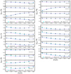 |
Fig. 3. Integrated-light NLTE abundance corrections for Na, Mg, Ca, Mn, and Ba. In each panel, corrections are shown as a function of [Fe/H] for three different abundance ratios, as indicated in the legends. |
For Mg, the NLTE corrections of all diagnostic lines display a rather smooth behaviour, not exceeding −0.03 dex at solar metallicity, but in the regime below [Fe/H] ≈ −1.5 some lines become more sensitive to NLTE effects. In particular, the strong Mg b triplet lines in the optical (5167 Å, 5172 Å, and 5183 Å) tend to become even stronger in NLTE at lower metallicity, however, we do not use these lines in this work. The profiles of the weaker high-excitation lines at 4572 Å, 4702 Å, 4731 Å, and 5711 Å remain either very close to LTE or are slightly weakened compared to LTE, which implies that the abundances derived from these lines in LTE are relative insensitive to NLTE effects. The NLTE corrections for the 5528 Å line are sensitive to the abundance of Mg at [Fe/H] = −2 and below. In the α-enhanced regime, [Mg/Fe] = +0.4 dex, which is typically seen in Galactic GCs, the line shows very small NLTE corrections. On the other hand, in α-poor conditions, [Mg/Fe] = −0.1 the NLTE correction is slightly negative.
The NLTE results for Ca depend on the properties of individual spectral lines. Whereas the overall behaviour is such that the NLTE line profiles are very similar to LTE at solar metallicity, [Fe/H] ≈ −1 represents a transition regime, where the NLTE corrections change sign and start increasing with decreasing metallicity. In the transition regime, the NLTE corrections are typically negative for all Ca I lines in our linelist, and reach −0.1 to −0.2 dex, depending on the abundance of Ca used in the statistical equilibrium calculations. The NLTE corrections are typically more negative for lower [Ca/Fe] ratios, and more positive for elevated [Ca/Fe]. In the most metal-poor systems, [Fe/H] ≲ −2, the NLTE corrections to abundances inferred from Ca I lines reach ∼0.1 dex and they become less sensitive to the Ca abundance in the model atmosphere.
Our results for Mn are very similar to those described in Eitner et al. (2020). Mn I is a typical low-ionisation-potential ion with large photo-ionisation cross-sections in the blue and it is subject to over-ionisation in the atmospheres of FGK-type stars. The NLTE corrections for all Mn I lines display a very similar behaviour, being close to +0.05 in solar-metallicity models, but they linearly increase with decreasing metallicity of the model. The largest NLTE correction of ∼ + 0.4 dex is attained at [Fe/H] = −3, which represents the limit of our model grid. This implies that Mn abundances in LTE are systematically under-estimated and the bias increases for more metal-poor systems.
The Ba II lines are qualitatively similar to the Na I lines in terms of their NLTE effects, which is not surprising because for both systems the NLTE effects are driven by strong line scattering. The NLTE corrections are small and slightly negative for the resonance line at 4554 Å and the weaker subordinate line at 5853 Å. Only in metal-poor models with extreme Ba enhancement ([Ba/Fe] = 0.8 dex) does the subordinate line show the NLTE correction of −0.2 dex. However, the 6141 Å and the 6496 Å lines show a larger sensitivity to NLTE, which is reflected in their NLTE corrections smoothly increasing in amplitude with decreasing metallicity. In the models with [Fe/H] ≲ −2, the corrections reach a plateau at ΔNLTE ≈ −0.2 dex and then start increasing again.
3.8. Validation on 47 Tuc
In L2017 the integrated-light analysis technique was tested by measuring metallicities and chemical abundances for the seven Galactic GCs that are also included here. In that paper, the sensitivity of the analysis to various model assumptions was also tested, and it is not our intent to repeat those tests here. An extensive discussion of systematic uncertainties in the analysis of integrated-light spectra can also be found in Sakari et al. (2014). Here, instead, we carry out a more detailed comparison with the well-studied Galactic GC 47 Tuc, for which measurements of a large number of elements for individual stars are available in the literature.
Table 3 lists our integrated-light abundance measurements for 47 Tuc and recent literature data. The measurements of MB2008 and Sakari et al. (2013, S2013) are integrated-light measurements, while those of Koch & McWilliam (2008, KM2008) and Thygesen et al. (2014, T2014) come from individual RGB stars. The T2014 analysis includes NLTE corrections for Na, Mg, and Ba. In addition to our default MF (α = −1), we list results for a Kroupa MF and for a flat (i.e. extremely bottom-light) MF (α = 0). We also include results obtained from a modelling based on a BaSTI isochrone, as well as the previous integrated-light measurements from L2017. The abundances in Table 3 are weighted averages of the values obtained from fits to the individual spectral windows,
![$$ \begin{aligned} \langle \mathrm{[X/Fe]} \rangle \equiv \frac{\sum { w}_i \mathrm{[X/Fe]}_i}{\sum { w}_i} \end{aligned} $$](/articles/aa/full_html/2022/04/aa42243-21/aa42243-21-eq13.gif)
Analysis of 47 Tuc.
with weights defined as

where σ0 = 0.05 dex is a ‘floor’ added in quadrature to account for non-random uncertainties on the abundances derived from the individual fits. For a discussion of the uncertainties on the integrated-light measurements we refer to Sect. 3.9, but here we note that the window-to-window dispersions for 47 Tuc are mostly fairly similar to those found in the analyses of the Sun and Arcturus.
The NLTE columns list the abundances obtained by applying the NLTE corrections to the DSEP and BaSTI α = −1 analyses. Comparison with Table 2 shows that the NLTE corrections for 47 Tuc are fairly similar to those obtained for Arcturus. Values in parentheses are elements for which no NLTE corrections were computed, but the abundance ratios relative to iron still change by −0.012 dex relative to the LTE values because of the change in [Fe/H].
A substantial range of iron abundances are quoted in the literature for 47 Tuc, spanning a range of at least 0.2 dex from [Fe/H] = −0.83 (Lapenna et al. 2014) to [Fe/H] = −0.62 (Pritzl et al. 2005). The most recent version of the Harris (1996) catalogue lists [Fe/H] = −0.72. Our new NLTE measurement, [Fe/H] = −0.74 for the reference MF ([Fe/H] = −0.72 when using the BaSTI isochrone), is thus in better agreement with the literature data than the analysis presented in L2017. It was found in L2017 that using the empirical CMD instead of theoretical isochrones to model the HRD of 47 Tuc had practically no effect on [Fe/H], and Table 3 shows that the effect of changing the MF is relatively minor, too. Most of the difference with respect to L2017 is due to a combination of the updated microturbulence prescription and the use of model atmospheres with self-consistent abundance patterns. While the line list used here also differs from that used in L2017, this only has a small effect on the iron abundance: repeating the same analysis as in L2017, but with our new line list, we found [Fe/H] = −0.855 (LTE) which differs by less than 0.01 dex from the value in L2017. The uncertainty on the iron abundance due to stochastic sampling of the MF within the slit scan area is about 0.04 dex (L2017).
A detailed discussion of integrated-light Na and Mg abundance measurements for the Galactic GCs was given in L2017. A complication affecting these elements is that their abundances often exhibit large star-to-star variations within individual GCs. In 47 Tuc, the range in [Na/Fe] is about 0.5 dex, but there is no significant spread in [Mg/Fe] (Carretta et al. 2009a, hereafter C2009). The LTE abundances of these elements found from our new analysis differ only slightly from those in L2017. For Mg, the integrated-light abundance ratio is unaffected by NLTE corrections, while the Na abundance is 0.16 dex lower in NLTE. Our [Mg/Fe] measurement agrees well with those found by other studies, with the exception of MB2008 whose integrated-light [Mg/Fe] value is about 0.2 dex lower. Our NLTE [Na/Fe] value agrees well with the studies of individual stars listed in Table 3, of which one (T2014) likewise included NLTE corrections and the other (KM2008) was a differential analysis with respect to the Sun. The two other literature integrated-light analyses (MB2008; S2013) both assumed LTE, and agree well with our measured LTE [Na/Fe] value.
While not listed in Table 3, it is also of interest to compare with the measurements of [Na/Fe], [Mg/Fe], and [Si/Fe] obtained from UVES spectra of 11 individual stars in 47 Tuc by C2009. They find a significantly higher mean NLTE Na abundance ratio of ⟨[Na/Fe]⟩= + 0.53 than that reported here. They also find a somewhat higher Mg abundance ratio (⟨[Mg/Fe]⟩= + 0.52), while their Si abundance ratio is similar to ours (⟨[Si/Fe]⟩= + 0.40). For Mg, the difference can be attributed to different atomic parameters and solar reference abundances, where their solar Mg abundance (from Gratton et al. 2003) is 0.15 dex lower than that used in our work. For Na, the difference is less easily explained. Part of it (0.12 dex) can again be explained by different solar reference abundances, but this still leaves a difference of about 0.2 dex unaccounted for. The spread in [Na/Fe] values within GCs in general, including 47 Tuc, contributes to some uncertainty on the mean value computed for a sample of only 11 stars, but seems unlikely to fully explain the 0.2 dex offset. Indeed, for a larger sample (147) of GIRAFFE spectra, Carretta et al. (2009b) quote a minimum [Na/Fe] = +0.15 and a maximum [Na/Fe] = +0.74 for member stars of 47 Tuc, and for this sample we compute a mean value of ⟨[Na/Fe]⟩= + 0.47, still considerably higher than our NLTE measurement and the literature values in Table 3. We return to this discrepancy below (Sect. 4.2).
The new spectral windows and the atomic data for Ca (Sect. 3.4) differ significantly from those used in our previous work, and our new LTE [Ca/Fe] measurement for 47 Tuc is about 0.1 dex lower than in L2017. In the comparisons with Arcturus and the Sun, our [Ca/Fe] measurements were slightly higher than the literature values, but for 47 Tuc our LTE measurement ([Ca/Fe] = +0.30 for α = −1) falls within the range of values determined by other authors. We note that the Ca abundance measurement is sensitive to the MF choice, with a difference of nearly 0.1 dex in [Ca/Fe] between the fits for a Kroupa and a flat (α = 0) MF. The NLTE corrections lead to a decrease of 0.06 dex in [Ca/Fe]. Hence it appears that specific model assumptions can have a relatively large systematic effect, at least ∼0.1 dex, on [Ca/Fe]. Other elements for which the spectral windows have changed significantly are Ti and Cr, but for these elements the resulting changes in the abundance ratios are smaller than for Ca and both fall within 0.05 dex of those determined in L2017.
We include several elements here that were not previously measured in L2017: Si, Ni, Cu, Zn, Zr, and Eu. Of these, our [Si/Fe] ratio agrees well with the literature data, while literature data are more scarce for the rest. Our LTE [Ni/Fe] measurement falls within 0.03 dex of that found by MB2008, while it is about 0.15 dex higher than the value found by T2014. For Zn, our LTE value ([Zn/Fe] = +0.13 ± 0.05) is 0.13 dex lower than that found by T2014 although the latter has a fairly large uncertainty (0.26 ± 0.13). Černiauskas et al. (2018) measured an average Zn abundance of ⟨[Zn/Fe]⟩= + 0.11 for 27 RGB stars in 47 Tuc (with an rms variation of 0.09 dex), which agrees well with our measurement. Despite the measurement of [Eu/Fe] being relatively challenging, our [Eu/Fe] value agrees well with those determined by T2014 and S2013, and we get very consistent results from the two Eu II lines (see Appendix F). There is a somewhat larger difference of about 0.2 dex with respect to MB2008.
For most elements, the results depend only weakly on the detailed HRD modelling assumptions. The strongest dependency on MF slope occurs for Ca, as mentioned above. For most other elements the effect is small, ∼0.01 dex. The same is true for the choice of isochrones, where the most strongly affected abundance ratios are [Zn/Fe], [Zr/Fe], and [Eu/Fe], which vary by ∼0.05 dex. Again, more typical variations are ∼0.01 dex.
3.9. Analysis of the globular cluster spectra
Our full sample of GC spectra were analysed using the same procedure as described above for NGC 104. For uniformity, we based all analyses on theoretical isochrones, even though resolved photometry reaching the main sequence turn-off is available for some clusters (mainly those in the Milky Way and Fornax dSph galaxies). In Table 4 we list the ages and compositions ([Fe/H] and [α/Fe]) for the isochrones used to model each cluster and the Galactic GCs from which HBs were adopted. Metallicities were chosen to self-consistently match those derived from the LTE spectral analysis to within a 0.1 dex tolerance. In most cases we assumed ages of 13 Gyr, but for the M 31 GCs we adopted the ages from Caldwell et al. (2011) and somewhat younger ages (10 Gyr) were assumed for several of the M 33 GCs on account of their relatively red HB morphologies (Sarajedini et al. 2000). The analysis in the remainder of this paper is based on DSEP isochrones for all clusters except M 31 EXT8, but results based on BaSTI isochrones are included in Appendix E. The DSEP isochrones do not extend to the low metallicity of M 31 EXT8 and we based the analysis of this cluster on a BaSTI isochrone, instead of using a MIST isochrone with scaled-solar composition as was done in Larsen et al. (2020). Table 4 also lists the Gaussian dispersions of the kernels used to smooth each spectrum and the heliocentric radial velocities. The latter are given to the nearest km s−1 and have typical uncertainties of about 1 km s−1.
Summary of model assumptions.
Figure 4 shows example fits for several GCs, ranging from the metal-poorest to the most metal-rich. Apart from the different metallicities, the figure also illustrates how the appearance of the spectra changes depending on the S/N (Table A.1) and the broadening of the spectra. For the spectra shown in the figure, the S/N (per Å) ranges from 81 (M 33 M9) to 394 (M 31 058−119) while the broadening is between 6.4 km s−1 (for M 33 M9) and 18.2 km s−1 (M 31 163−217). The broadening is dominated by internal velocity broadening in the clusters but also includes the instrumental broadening of 2−3 km s−1.
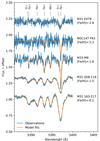 |
Fig. 4. Integrated-light spectra and model fits for GCs spanning the range of NLTE metallicities from [Fe/H] = −2.8 (M 31 EXT8, top) to [Fe/H] = −0.1 (M 31 163−217, bottom). |
The individual abundance measurements for each spectral window are listed in Appendix F. For each window we list the wavelength range, the LTE abundance obtained from the spectral fitting ([X/H](LTE)), the NLTE correction ΔNLTE, and the uncertainty σi on the measurement. The weighted average abundance measurements are listed in Tables C.1–C.3 and include the NLTE corrections for the elements for which these were computed (the pure LTE versions are listed in Tables D.1–D.3). The formal uncertainties on the average measurements (σ⟨X⟩), based on propagation of the measurement errors, were computed as
with weights wi defined by Eq. (7). The total uncertainties on the mean abundance ratios [X/Fe] should, in principle, be estimated as ![$ \sigma_{\langle{\rm [X/Fe]}\rangle}^2 = \sigma_{\langle{\rm X}\rangle}^2 + \sigma_{\langle{\rm Fe}\rangle}^2 $](/articles/aa/full_html/2022/04/aa42243-21/aa42243-21-eq16.gif) , but in practice the (random) uncertainties on the Fe abundances are almost always much smaller than for the other elements. However, in most cases the scatter of the measurements exceeds the formal uncertainties, so that a propagation of the measurement errors underestimates the true uncertainties. In these cases, a more conservative estimate of the errors comes from the weighted standard deviations,
, but in practice the (random) uncertainties on the Fe abundances are almost always much smaller than for the other elements. However, in most cases the scatter of the measurements exceeds the formal uncertainties, so that a propagation of the measurement errors underestimates the true uncertainties. In these cases, a more conservative estimate of the errors comes from the weighted standard deviations,
![$$ \begin{aligned} \mathrm{SD}_{X,{ w}} \equiv \left[\frac{N}{N-1} \frac{\sum \left(\mathrm{[X/Fe]}_i - \langle \mathrm{[X/Fe]} \rangle \right)^2 { w}_i}{\sum { w}_i}\right]^{1/2} \end{aligned} $$](/articles/aa/full_html/2022/04/aa42243-21/aa42243-21-eq17.gif)
from which the standard errors on the mean can then be estimated as  , where N is the number of measurements. We list both estimates of the uncertainties, except when N = 1 in which case SDX, w is undefined. In most cases, SX > σ⟨X⟩, but in a few cases the opposite is true, typically for small N where the estimate of SX may not be very reliable.
As discussed in Sect. 3.5.1, the uncertainties on the [Eu/Fe] measurements are correlated with those on [Ca/Fe]. More generally, we may expect correlations between the errors on different abundance ratios. In the case of Eu and Ca, the reason is easily identifiable as line blending, so that an increase in [Ca/Fe] leads to a decrease in [Eu/Fe]. However, more subtle inter-correlations may result from variations in the atmospheric structure, such as may be caused by variations in the abundances of important electron-donor elements (e.g. Na, Mg, and Si). It is not computationally practical to quantify these effects fully for each individual cluster, but in Tables 5 and 6 we illustrate the effect of varying the abundances of a subset of the elements by 0.1 dex, taking NGC 104 and NGC 7078 as representative of metal-rich and metal-poor GCs. The error correlations are quite modest for most elements, the most significant (anti-)correlation indeed being that of Eu vs. Ca. In general, these interdependencies are not symmetric; a change in the Ca abundance has a much larger effect on Eu than vice versa, because the Ca measurement is based on many more, stronger lines.
Error correlations for NGC 104.
Error correlations for NGC 7078.
Figure 5 shows the NLTE abundance corrections per element as a function of metallicity for each cluster, averaged over all spectral windows. For some elements, NLTE corrections are not available for all spectral windows and in these cases the missing corrections were estimated as the weighted average of the available corrections. The NLTE corrections are plotted for the abundances relative to hydrogen (ΔNLTE([X/H]) so that the corrections on the abundance ratios with respect to iron are given as ΔNLTE([X/Fe]) = ΔNLTE([X/H])−ΔNLTE([Fe/H]). For iron, the corrections are very small at the high metallicity end (ΔNLTE([Fe/H] ≈ +0.01 dex) and gradually increase towards lower metallicities, reaching ΔNLTE([Fe/H]) = + 0.07 dex for M 31 EXT8 at [Fe/H](LTE) = − 2.9. The corrections for Na are fairly constant at ΔNLTE([Na/H])≈ − 0.1 and most closely resemble the corrections for the 5688.193 Å line, which carries the most weight in the fits. For Mg the corrections are very small, although the variations in the corrections for iron introduce a trend of slightly decreasing [Mg/Fe] NLTE abundances, compared to the LTE values, towards the low-metallicity end. For Ca and Ti the trends with wavelength are similar to that for iron, so that the slope of [Ca/Fe] and [Ti/Fe] versus [Fe/H] looks similar in NLTE and LTE, although the corrections for Ti are more positive (by ≈0.15 dex) overall. As found in previous studies, the corrections for Mn increase strongly towards low metallicities, and a significant trend is seen also for Ni. For Ba the corrections are slightly negative, decreasing by about 0.1 dex from high to low metallicities.
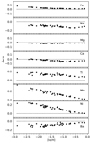 |
Fig. 5. Average integrated-light NLTE corrections for each element as a function of metallicity. |
A more detailed comparison of LTE and NLTE abundances is given in Table 7 for NGC 104 and NGC 7078. For each NLTE element we list the abundance correction ΔNLTE and the weighted standard deviations of the LTE and NLTE measurements. The general trends with metallicity noted above are again apparent from this table. The correction for iron is very small for NGC 104 (+0.01 dex) and increases to +0.05 dex for NGC 7078. In both cases, the dispersions SDFe, w on [Fe/H] remain the same, which is a consequence of the relatively small dispersion in the corrections themselves (σNLTE([Fe/H]) = 0.01 dex for NGC 104 and σNLTE([Fe/H]) = 0.039 dex for NGC 7078) compared to the overall spread in the abundance measurements between the different windows. Except for Na, all corrections are smaller than 0.1 dex for NGC 104, while larger corrections are found for NGC 7078 for several elements. With a few exceptions, the dispersions SDX, w decrease for the NLTE abundances, which reinforces the need to account for NLTE effects in accurate studies of chemical abundances of stellar populations.
Comparison of LTE and NLTE abundances for NGC 104 and NGC 7078.
In Fig. 6 we compare our integrated-light [Fe/H] measurements with data for GCs in the Milky Way (Harris 1996, 2010 revision) and M 31 (Caldwell et al. 2011). The former are based on data compiled from the literature while the latter are based on measurements of Lick indices on Hectospec data. To be consistent with the literature data, which are mostly based on LTE analyses (ultimately tied to the C2009 and Carretta & Gratton 1997 abundance scales), we plot our LTE measurements in this figure. The straight line represents the one-to-one relation and is not a fit to the data. We see that our measurements agree well with the literature data, with a standard deviation around the 1:1 relation of 0.09 dex. The mean metallicity offset between our measurements and those listed in Harris (1996) is ⟨Δ[Fe/H]⟩MW = 0.001 dex, while for M 31 it is ⟨Δ[Fe/H]⟩M 31 = 0.029 dex. For the combined sample we find ⟨Δ[Fe/H]⟩All = 0.017 dex. If we instead compare with our NLTE abundances, the offset for the combined sample increases to 0.037 dex. Overall, then, the cluster metallicities derived from our integrated-light analysis agree well with existing data for these well-studied clusters, with no evident systematic trends as a function of metallicity.
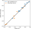 |
Fig. 6. Comparison of our integrated-light LTE [Fe/H] values for M 31 and Milky Way GCs with data from Caldwell et al. (2011) and Harris (1996). The line is the 1:1 relation, not a fit. |
In addition to the detailed comparison of literature data carried out for NGC 104 in Sect. 3.8, it is of interest to compare our abundance measurements for Galactic GCs with the NLTE analysis by Kovalev et al. (2019, K2019). These authors measured abundances for individual stars in four GCs in common with our sample, namely NGC 104, NGC 362, NGC 6752, and NGC 7078. We list their average NLTE measurements of [Fe/H], [Mg/Fe], and [Ti/Fe], together with our own NLTE measurements (from Table C.1) in Table 8. For all clusters except NGC 6752, the [Fe/H] values are in agreement to within 0.02 dex. The case of NGC 6752 has been discussed in L2017, where it was noted that the relatively low surface brightness and large diameter on the sky make the integrated-light spectrum of this cluster especially susceptible to stochastic fluctuations in the number of red giants. This causes a stochastic uncertainty of 0.1 dex in [Fe/H] for this cluster, which is not included in the uncertainty in Table 8. The [Mg/Fe] values agree within the uncertainties, while our [Ti/Fe] values tend to be somewhat higher (by 0.1−0.2 dex) than those of K2019, which is likely due to us using an updated and more accurate NLTE model atom of Ti in this work.
Comparison of our integrated-light NLTE abundance measurements with NLTE measurements for individual stars (Kovalev et al. 2019, K2019).
4. Results
We next give an overview of previous work on the GC systems in the galaxies included in our sample and discuss various aspects of the analysis specific to each galaxy.
4.1. Remarks on globular cluster systems of individual galaxies
Fornax. The GC system of the Fornax dSph has an interesting history. The brightest cluster, Fornax 3, was discovered long before the Fornax dwarf itself by John Herschel, who described it as ‘a curious little object and easily mistaken for a star, which, however, it certainly is not’ (Herschel 1847). Shapley (1939) added the clusters now generally referred to as Fornax 2 and Fornax 4 and also listed ‘a very faint cluster of unidentified character’. This description of Fornax 6 remains quite appropriate today, although spectroscopic observations indicate that it is more metal-rich ([Fe/H] = −0.71 ± 0.05), and probably younger, than the other clusters (Pace et al. 2021). Clusters 1 and 5, the outermost known clusters, were discovered by Hodge (1961). Fornax 1 and 2 are relatively extended, diffuse objects, not ideal for our integrated-light measurements, but from high-dispersion spectroscopy of individual stars these clusters were found to be metal-poor ([Fe/H] = −2.5 and −2.1, respectively) and α-enhanced (Letarte et al. 2006).
The metallicities measured here for Fornax 3 ([Fe/H] = −2.28 ± 0.02) and Fornax 5 ([Fe/H] = −2.06 ± 0.03) are very similar to those determined in our previous work, while our new determination of [Fe/H] = −1.24 ([Fe/H] = −1.26 in the LTE analysis) for Fornax 4 is 0.10−0.15 dex higher (Larsen et al. 2012, 2018a). Within a projected galactocentric radius of 0.6°, approximately corresponding to the location of the outermost GCs, the field star metallicity distribution in Fornax is instead dominated by a component with [Fe/H] ≃ −1 (Battaglia et al. 2006; Kirby et al. 2011). While this component becomes less prominent beyond 0.6° (Hendricks et al. 2014), the conclusion that the GCs (except Fornax 6) are significantly more metal-poor than the bulk of the field stars in Fornax thus remains unchanged. Fornax 3 and Fornax 5 are (again) found to be moderately α-enhanced, and the α-element abundances of Fornax 4 remain close to scaled-solar.
Fornax 3 was included in the integrated-light study by Colucci et al. (2017), who found a metallicity very similar to ours ([Fe/H] = −2.27 ± 0.05 from Fe I). They also reported enhanced α-element abundances ([Mg/Fe] = +0.21 ± 0.22, [Ca/Fe] = +0.24 ± 0.10, [Ti I/Fe] = +0.29 ± 0.06, and [Ti II/Fe] = +0.35 ± 0.10) that are consistent with our LTE values, although they found a somewhat lower Ba abundance ([Ba/Fe] = +0.12 ± 0.08) than our measurement.
While we have assumed an age of 13 Gyr for Fornax 4, some studies have reported a somewhat younger age of ∼10 Gyr (Buonanno et al. 1999; Hendricks et al. 2016; Martocchia et al. 2020). Indeed, a younger age would be consistent with the less α-enhanced composition. Repeating our analysis for an age of 10 Gyr instead of 13 Gyr makes little difference, with [Fe/H] increasing very slightly (by 0.006 dex) and the α-element abundance ratios changing by 0.01−0.02 dex.
The composition and nature of Fornax 4 have been subjects of some debate in the literature. Strader et al. (2003) found [Fe/H] = −1.5 and listed literature metallicities ranging between [Fe/H] = −2.0 and [Fe/H] = −1.35. Some of these values are based on measurements of various spectral features that are sensitive not only to Fe, but also to elements such as Ca and Mg. Given that the conversions from line strengths and/or indices to metallicities in some of these studies are calibrated on Galactic GCs that tend to have α-enhanced abundance patterns (Brodie & Huchra 1990; Dubath et al. 1992), the resulting metallicities may be biased by the scaled-solar abundance patterns in Fornax 4. Hendricks et al. (2016) measured [Fe/H] = −1.50 ± 0.05 for one likely member star, again somewhat lower than our measurement. Their α-element abundances were largely consistent with the roughly scaled-solar composition found from our measurements, but with large uncertainties ([Si/Fe] = −0.35 ± 0.34, [Ca/Fe] = +0.05 ± 0.08, and [Ti/Fe] = −0.27 ± 0.23).
Despite a small radial velocity offset (6−9 km s−1; Larsen et al. 2012; Hendricks et al. 2016) between Fornax 4 and the field stars, the location of the cluster near the centre of the Fornax dSph has led to suggestions that it may be the nucleus (Hardy 2002; Strader et al. 2003). This idea has recently been revisited by Martocchia et al. (2020), who found a larger colour spread on the RGB than could be accounted for by the measurement errors, suggesting a metallicity spread of up to ≈0.5 dex. While this should not seriously affect the comparison of integrated-light measurements, a robust comparison with individual stars would require larger samples than the single star of Hendricks et al. (2016).
Wolf-Lundmark-Melotte. The WLM galaxy hosts a single known, but quite luminous (MV = −9), GC (Humason et al. 1956; Sandage & Carlson 1985; Larsen et al. 2014). A CMD from the Hubble Space Telescope (HST) shows well-defined giant- and horizontal branches, and confirms the object as an old, metal-poor GC (Hodge et al. 1999). Our measurement of the iron abundance, [Fe/H] = −1.85 ± 0.03, is about 0.11 dex higher than that listed in Larsen et al. (2014), which is mainly due to the revised microturbulence prescription and the inclusion of NLTE corrections. However, it is still significantly lower than that listed by Colucci & Bernstein (2011) who found [Fe/H] = −1.71 ± 0.03. In any case, the GC in WLM has a metallicity well below that of the general old field population, which has an average [Fe/H] = −1.3 (Leaman et al. 2013). Similar to Fornax, WLM is thus in agreement with the general tendency for GCs to preferentially be associated with the more metal-poor populations in their parent galaxies (Forte et al. 1981; Brodie & Huchra 1991; Harris et al. 2007; Lamers et al. 2017). Colucci & Bernstein (2011) also found [Ca/Fe] = +0.25 ± 0.05 and [Ba/Fe] = −0.05 ± 0.15, which agrees well with our measurements.
NGC 147. This M 31 satellite galaxy has ten known GCs. Six of these were discovered relatively recently, with three each by Sharina & Davoust (2009) and Veljanoski et al. (2013) who also provide a review of the earlier literature on the GC system in NGC 147, going back to Baade (1944).
Our observations of GCs in NGC 147 were previously presented in Larsen et al. (2018a). The metallicities derived here are slightly higher than those found previously (∼0.1 dex), due to the updated assumptions in our modelling procedure which also lead to slight changes in the abundances of individual elements. The overall conclusions remain unchanged, that is, the GCs are more metal-poor than the bulk of the field stars in NGC 147 and the α-element abundances are generally similar to those of Milky Way GCs and field stars at similar metallicities. For Hodge III, [Mg/Fe] remains lower than the other α-element abundance ratios, which now also include [Si/Fe]. As discussed in more detail below (Sect. 4.2), the abundances of Mg deviate from those of other α-elements in several other GCs in our sample.
NGC 185. As in NGC 147, the presence of GCs in NGC 185 was first noted by Baade (1944). Today, a total of eight GCs are known in NGC 185 (Veljanoski et al. 2013). Interestingly, the three GCs that we have observed in this M 31 companion all have nearly identical [Fe/H] ≃ −1.75, and the α-elements (Si, Ca, and Ti) are enhanced by similar amounts as in Milky Way GCs at this metallicity. Larger variations are seen in the abundances of Na and Mg, perhaps related to the presence of multiple populations.
Among the clusters observed here, FJJ-III and FJJ-V were also included in the sample of Da Costa & Mould (1988), whose determinations of the iron abundances are very similar to ours ([Fe/H] = −1.7 ± 0.15 for FJJ-III and [Fe/H] = −1.8 ± 0.15 for FJJ-V). All three GCs observed here are in common with the study by Sharina et al. (2006), who found metallicities of [Z/H] = −1.6 ± 0.3 (FJJ-III), −1.5 ± 0.2 (FJJ-V), and −1.5 ± 0.3 (FJJ-VIII). They also measured α-element abundance ratios of [α/Fe]= + 0.1 ± 0.3, 0.0 ± 0.3, and 0.0 ± 0.3, for the three clusters. There is a tendency for these [α/Fe] ratios to be closer to solar than indicated by our measurements, although the results for individual clusters are largely consistent with our α-enhanced values within the relatively large uncertainties on the Sharina et al. (2006) measurements. It is less clear how to compare their total metallicities, [Z/H], with our measurements of [Fe/H]. If we use the relation [Fe/H] = [Z/H] − 0.75 × [Mg/Fe] (Vazdekis et al. 2015) to convert our [Fe/H] values to [Z/H] by adding a rough correction of +0.2 dex (assuming [Mg/Fe] ≈ 0.3) they become similar to the [Z/H] values obtained by Sharina et al. (2006), although this procedure may be questionable given the roughly scaled-solar α-element abundances found by the latter study.
NGC 205. The current list of known GCs in NGC 205 has changed little with respect to the eight objects identified by Hubble (1932). Hubble III has a radial velocity that suggests it is most likely a projected M 31 GC and Hubble V may be an intermediate-age object. An additional candidate listed by Sargent et al. (1977), M 31C-55, has subsequently been identified as a foreground star (Battistini et al. 1987; Da Costa & Mould 1988; Galleti et al. 2004) and indeed has a non-zero proper motion according to Gaia EDR3 (pm(RA, Dec) = (−0.47 ± 0.11, −0.96 ± 0.10) mas yr−1) which would imply a velocity of about 4000 km s−1 at the distance of NGC 205.
The two GCs included in our sample, Hubble I and Hubble II, both have enhanced α-element abundance ratios according to our analysis. Our metallicity determinations of [Fe/H] = −1.41 ± 0.03 (Hubble I) and [Fe/H] = −1.35 ± 0.02 (Hubble II) agree fairly well with those by Da Costa & Mould (1988), [Fe/H] = −1.5 ± 0.15 for both clusters, and with the value of [Fe/H] = −1.49 ± 0.02 found for Hubble I by Colucci & Bernstein (2011). The latter authors also found both clusters to be α-enhanced, although they found a somewhat higher metallicity for Hubble II ([Fe/H] = −1.12 ± 0.02). Sharina et al. (2006) found relatively high metallicities for both clusters ([Z/H] = −1.1 ± 0.1 for Hubble I and [Z/H] = −1.2 ± 0.1 for Hubble II) and lower α-element abundance ratios ([α/Fe]= + 0.2 ± 0.2 and [α/Fe] = 0.0 ± 0.2).
NGC 6822. Hubble (1925) listed ten ‘nebulae’ in NGC 6822, of which he tentatively suggested that a few might be stellar clusters. One of these, Hubble VII, was confirmed as an old, metal-poor GC by Cohen & Blakeslee (1998), who found an age of  Gyr and a metallicity of [Fe/H] = −1.95 ± 0.15 dex from spectroscopic line index measurements. A CMD obtained from HST data is also consistent with that of an old, relatively metal-poor GC (Wyder et al. 2000). An additional seven GCs, located outside the main body of NGC 6822, were discovered more recently on ground-based wide-field CCD images (Hwang et al. 2011; Huxor et al. 2013).
Our analysis of the clusters SC6 and SC7 was discussed in Larsen et al. (2018a). As for most other clusters that we have reanalysed here, the metallicities have increased by about 0.1 dex (mainly due to the revised microturbulence prescription), but we recover our previous result that the α-element abundances for SC7 are close to scaled-solar while SC6 exhibits the α-enhanced abundance patterns that are characteristic of other metal-poor GCs in our sample.
In addition to SC6 and SC7, we here include the cluster Hubble VII although the analysis of its spectrum posed some difficulties. When plotting the abundance measurements as a function of wavelength, the spectral windows with wavelengths λ > 5200 Å tended to yield higher Fe abundances than the bluer windows. Specifically, using only windows with λ < 5200 Å we found [Fe/H] = −1.77 (with an rms of 0.13 dex) while for λ > 5200 Å we found [Fe/H] = −1.58 (rms 0.23 dex). Such a trend could potentially be caused by a mismatch between the HRD of the actual cluster and that used in the modelling, for example if an incorrect age were assumed. However, the trend persisted even if an age as young as 5 Gyr was assumed: in this case we still found a difference of 0.16 dex between the [Fe/H] values for λ < 5200 Å and λ > 5200 Å.
As Hubble VII is projected onto the main body of NGC 6822, where the background is more complicated, one might suspect poor background subtraction as a possible culprit. We compared our HIRES spectrum with a spectrum obtained with the Keck Cosmic Web Imager (KCWI) and found the two spectra to be very similar (apart from the lower spectral resolution of KCWI). Hence, we have not been able to identify a satisfactory explanation for the difficulties with the analysis of Hubble VII, and the results should therefore be considered more uncertain than for the other clusters in our sample. Nevertheless, our analysis agrees fairly well with that of Colucci & Bernstein (2011) who measured [Fe/H] = −1.61 ± 0.02, just 0.06 dex higher than our value (or 0.08 dex when compared with our LTE analysis). In both cases, these are significantly higher iron abundances than the value measured by Cohen & Blakeslee (1998). Colucci & Bernstein (2011) also found an approximately scaled-solar Ca abundance of [Ca/Fe] = +0.01 ± 0.07, which is similar to our measurement of [Ca/Fe] = +0.07 ± 0.04 (+0.06 in LTE). Nevertheless, the detailed abundance patterns remain somewhat puzzling, as we find Si and Ti to be enhanced while Mg is depleted (−0.03 dex). We also find a slightly higher Ba abundance than Colucci & Bernstein (2011), [Ba/Fe] = +0.35 ± 0.08 dex (+0.48 in LTE) vs. their [Ba/Fe] = +0.22 ± 0.13. Hubble VII thus appears worthy of further study.
M 31. Since the initial discovery of 140 ‘nebulous objects …provisionally identified as globular clusters’ by Hubble (1932), the M 31 GC system has been the subject of numerous studies. We do not attempt to review the literature here, but only note that the spectroscopic observations analysed here were made prior to the identification of about 100 GCs in the PAndAS survey, mostly located in the outer halo of M 31 (Huxor et al. 2014). Many of these are, in any case, relatively extended, and therefore less efficiently observed with a single-slit spectrograph such as HIRES.
The M 31 GCs in our sample span a NLTE metallicity range from [Fe/H] = −2.8 (EXT8) to [Fe/H] = −0.1 (163−217). They all show enhanced abundances of Si, Ca, and Ti relative to scaled-solar composition, although EXT8 is extremely Mg-deficient (Larsen et al. 2020). In general, the abundance patterns tend to align with those observed in Milky Way GCs of similar metallicities. From integrated-light spectroscopy, the inner ∼10′ of M 31 itself are dominated by old, α-enhanced ([α/Fe]≃0.25) stars with near-solar metallicities, associated with a bulge or bar-like component (Saglia et al. 2009, 2018). Hence, the enhanced α-element abundances of the metal-rich GCs are similar to those seen in metal-rich stars in the central regions of M 31 and may trace the same components at larger galactocentric distances. The three most metal-rich M 31 GCs in our sample are located at projected distances of  (171−222),
  (163−217), and
  (225−280).
The clusters analysed here are among the brightest GCs in M 31, and many of them have been included in several spectroscopic studies in the past. In addition to the comparison with the low-dispersion metallicity measurements in Fig. 6, it is of interest to compare with previous analyses that made use of high-dispersion spectroscopy and analysis techniques similar to ours. In Table 9 we compare our LTE abundance measurements with those published by Colucci et al. (2014, C2014), also using HIRES observations (but from different runs than those used here) and Sakari et al. (2016, S2016) (using APOGEE H-band observations). We do not include the errors on the measurements in Table 9 but they typically amount to ∼ ± 0.1 dex (see Tables C.1–C.3 and the original references).
Comparison of our LTE measurements for M 31 GCs with literature data.
As noted by C2014, their measurements of [Fe/H] show a systematic difference with respect to low-resolution studies in the sense that their [Fe/H] values tend to be lower for metal-rich GCs. As discussed above (Sect. 3.9), we instead find excellent agreement between our iron abundances and those measured by Caldwell et al. (2011) at all metallicities, so that our [Fe/H] values are systematically higher than those of C2014 and S2016 at the high-metallicity end. At low metallicities (012−064 and 358−219), all three studies agree well on [Fe/H].
Despite the systematic differences in the iron abundances, we generally find similar abundance ratios to those measured by C2014 and S2016. There are some occasional outliers, such as [Na/Fe] and [Si/Fe] for 012−064 (where our measurements differ by 0.3−0.4 dex from those of C2014 and S2016) and [Mg/Fe] for 225−280, where the value measured by C2014 is about 0.2 dex higher, but otherwise the three studies mostly agree within ∼0.1 dex.
M 33. The characterisation of the M 33 GC system is, to a large extent, still a work in progress. Part of the difficulty stems from the fact that the GC population is relatively sparse (certainly when compared to that of M 31), and most of the clusters appear projected onto the highly structured disc of M 33. This difficulty is compounded by the presence of a large number of intermediate-age clusters which may easily be confused with ancient GCs, especially if reddened. Indeed, the prevalence of clusters with blue colours compared to Galactic GCs was noted already in early studies (Hiltner 1960; Kron & Mayall 1960) and was later confirmed by larger samples (Melnick & D’Odorico 1978; Christian & Schommer 1982).
Our sample of M 33 GCs mostly consists of clusters with resolved HST photometry from Sarajedini et al. (2000), to which we have added CBF 28 (Chandar et al. 1999) and the cluster HM33-B from Huxor et al. (2009). We had planned to include several additional GC candidates from Beasley et al. (2015) which however turned out to be Galactic foreground stars, as confirmed by their non-zero parallaxes and proper motions listed in the Gaia DR2 catalogue (IDs 1115, 1138, 1322, 1965, 2001, and 2145 in Beasley et al. 2015). The observations of the four clusters R14, U77, CBF 28, and HM33-B are published here for the first time, while analysis of data for H38, M9, R12, and U49 was included in Larsen et al. (2018a).
Despite the suggestion that the M 33 GCs are several Gyr younger than their Milky Way counterparts (Sarajedini et al. 2000), most of them have enhanced α-element abundances similar to those seen in GCs in other galaxies. However, it is interesting to note that HM33-B appears chemically more similar to Fornax 4 and NGC 6822-SC7 in some respects (we discuss this further in Sect. 5), and is also one of a few GCs located well outside the main body of M 33 (Huxor et al. 2009). This is reminiscent of the behaviour of stars in the outer M 31 halo, which also tend to have abundances more similar to those seen in dwarf galaxies (Gilbert et al. 2020).
NGC 2403. At a distance of about 3.2 Mpc (Freedman & Madore 1988; Radburn-Smith et al. 2011), this low-mass Sc-type spiral (similar to M 33) is the only galaxy in our sample that is located outside the Local Group. A list of five cluster candidates was given by Tammann & Sandage (1968), of which one had a red colour consistent with it being a GC. The cluster included in our sample, F46, was first identified by Battistini et al. (1984), who listed a relatively blue colour (B − V = 0.47) and suggested that it might be an intermediate-age object. However, according to SDSS DR12 photometry (Alam et al. 2015), F46 has (g − z)0 = 0.92 ± 0.02, which is quite normal for an old GC with a metallicity around [Fe/H] ≃ −1.5 (Vanderbeke et al. 2013).
The spectrum of F46 is of good quality, despite the relatively modest integration time (Table A.1) and most elemental abundances are well constrained. It helps that the cluster is very compact and the spectrum was obtained on a night with good seeing ( FWHM), so that slit losses were minimised. The cluster is moderately metal-poor ([Fe/H] = −1.71 ± 0.03) and the α-elements are mostly enhanced, with the exception of [Mg/Fe] which is sub-solar. In this respect F46 resembles several other clusters with metallicities around [Fe/H] ≈ −1.7.
We can use the velocity broadening obtained from the spectral analysis to constrain the virial mass and mass-to-light ratio of F46. Correcting the total broadening in Table A.1 for an instrumental broadening of 3.4 km s−1 (Larsen et al. 2020), the line-of-sight velocity broadening is σ1D = 11.7 km s−1. We used an HST/ACS archival image in the F555W filter (Progr. ID 10402, P.I. R. Chandar) to estimate the half-light radius of F46 by measuring the flux in concentric apertures. Visually, the cluster can be traced out to a radius of about 50 pixels ( ) in the ACS image, and within this radius the total magnitude is about mF555W = 17.8, slightly brighter than the value of V = 17.96 given by Battistini et al. (1984). The ACS photometry may however be affected by multiple cosmic-ray hits in the single exposure. Correcting the measurement in the ACS image for a foreground extinction of AV = 0.11 mag (NED) we get MV = −9.8. Half of the flux is contained within a radius of 6 ACS pixels or
  , corresponding to a half-light radius of rh = 4.6 pc at a distance of 3.2 Mpc. Subtracting the half-light radius of the ACS point-spread function (about 1.5 pixels; Bohlin 2016) in quadrature decreases rh by about 0.15 pc. The dynamical mass is then
and the mass-to-light ratio is Mdyn/LV ≃ 2.0 M⊙/LV, ⊙, which is a typical value for an old GC at this metallicity (Strader et al. 2011). For an age of 108 − 109 years, as suggested by Battistini et al. (1984), the V-band mass-to-light ratio would be only 5%−15% of that at 10 Gyr (e.g. Bruzual & Charlot 2003), in strong contrast to the measured value. We conclude that F46 is indeed most likely a relatively metal-poor, old GC.
4.2. Abundance trends
Having discussed the individual GC systems, we next turn to a more general discussion of the abundance trends and comparison with existing measurements of individual stars. In Figs. 7–10 we plot the measurements in Tables C.1–C.3 as a function of [Fe/H]. In each figure, the symbols for our integrated-light measurements are colour-coded according to the type of host galaxy, using the same scheme as in Fig. 1. Red symbols indicate GCs belonging to dwarf spheroidals and ellipticals (NGC 147, NGC 185, NGC 205, and the Fornax dSph) and teal-colour symbols indicate dwarf irregulars (NGC 6822 and WLM). The Milky Way, M 31, and M 33 GCs are shown with black, violet, and blue squares, respectively, and the single GC in NGC 2403 is represented by an orange square.
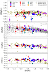 |
Fig. 7. Integrated-light abundances of α-elements relative to iron (Table C.1). Large symbols show our measurements, with symbol colours and shapes encoding information about the host galaxies as indicated in the legend. Error bars indicate σ⟨X⟩ or SX, whichever is larger. Olive coloured small triangles: NLTE measurements for Milky Way field stars (Bergemann et al. 2017b; Mashonkina et al. 2017b, 2019; Mishenina et al. 2017; Zhao et al. 2016). Orange points: Milky Way bulge stars (Bensby et al. 2017). Grey points in panel with [Si/Fe]: LTE measurements for Milky Way field stars (Suda et al. 2008). |
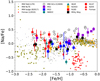 |
Fig. 8. Sodium abundances (NLTE). Symbols for our integrated-light measurements are the same as in Fig. 7. References for Milky Way GCs (open circles), Milky Way field star LTE data (grey points) and NLTE data (olive coloured triangles), and field stars in the Fornax dwarf (small red circles) are given in the text. |
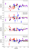 |
Fig. 9. Abundances of iron-peak elements (Table C.2). Symbols for our measurements are the same as in Fig. 7. NLTE abundances for Mn in Milky Way field stars are from Eitner et al. (2020). |
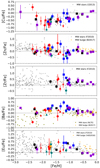 |
Fig. 10. Abundances of heavy elements (Table C.3). Symbols for our measurements are the same as in Fig. 7. |
The α-elements. Figure 7 shows the α-element abundance ratios ([Mg/Fe], [Si/Fe], [Ca/Fe], and [Ti/Fe]). Although the classification of Ti as an α-element may be questionable (Woosley & Weaver 1995), it usually tends to trace other α-elements (such as Mg and Si) fairly closely (Conroy et al. 2014; Parikh et al. 2019), and here we group it together with the α-elements. For Mg, Ca, and Ti we include NLTE measurements for Milky Way field stars (Zhao et al. 2016; Mashonkina et al. 2017b, 2019; Mishenina et al. 2017) and additionally, for Mg, data for 326 thick-disc stars from Bergemann et al. (2017b). For Si (where our measurements are LTE values) we show literature data from the Stellar Abundances for Galactic Archeology (SAGA) database (Suda et al. 2008). The increasing scatter at metallicities below [Fe/H] = −2 for the literature [Si/Fe] data is caused partly by larger measurement uncertainties, although uncertainties are not provided for all stars. We also include measurements for microlensed Milky Way bulge stars from Bensby et al. (2017) and literature data for individual stars in Galactic GCs (Roediger et al. 2014, R2014), the latter indicated with open circles.
Perhaps the most notable feature of Fig. 7 is the high degree of uniformity of the abundance patterns for Si, Ca, and Ti. All three elements are enhanced relative to scaled-solar composition with mean abundance ratios of ⟨[Si/Fe]⟩= + 0.32 ± 0.01, ⟨[Ca/Fe]⟩= + 0.21 ± 0.01, and ⟨[Ti/Fe]⟩= + 0.35 ± 0.01. The dispersions of the [Ca/Fe] and [Ti/Fe] values are only 0.09 dex and 0.10 dex, respectively, while the [Si/Fe] values have a larger dispersion (0.17 dex), driven at least in part by the larger uncertainties. Above [Fe/H] ≈ −0.5, [Ca/Fe] shows a declining trend towards higher metallicities while Ti and Si remain elevated throughout the entire metallicity range. We thus confirm the α-element like behaviour of Ti.
Overall, the abundance ratios [Si/Fe], [Ca/Fe], and [Ti/Fe] for our sample are fairly similar to those seen in the R2014 data and in the Milky Way field stars. The larger differences for Mg are discussed in more detail below. We note that the NLTE corrections tend to slightly decrease our [Ca/Fe] values and increase the [Ti/Fe] values (Table 7). There may indeed be a tendency for our abundances for these elements to be slightly offset in the corresponding directions from the R2014 data, which are generally based on LTE analyses of individual GC member stars. Slight offsets could, however, also be caused by other effects, such as differences in the atomic data and adopted solar abundance scales (Sect. 3.5.2). In their compilation, R2014 did not attempt to homogenise the data to account for such differences.
Superimposed on the general homogeneity of the α-element abundance patterns are some higher-order differences. Two GCs, Fornax 4 and NGC 6822-SC7, have consistently low α-element abundances. As discussed in Larsen et al. (2018a), this mirrors the tendency for the ‘knee’ in the α-element versus [Fe/H] relation to occur at a lower metallicity in dwarf galaxies than in the Milky Way. Our present sample includes an additional cluster with a hint of this behaviour, HM33-B, albeit at lower significance. This cluster has relatively low [Mg/Fe] and [Ca/Fe] ratios although the [Si/Fe] and [Ti/Fe] ratios are more similar to those of the Galactic stars at this metallicity. The S/N of the HM33-B spectrum is relatively low, and the uncertainties on the abundances thus relatively large, and obtaining a better spectrum of this cluster would be desirable. At metallicities below those of Fornax 4, NGC 6822-SC7, and HM33-B, [Fe/H] < −1.3, there is a small but systematic difference between the mean α-element abundance ratios for the GCs in spirals and those in dwarf galaxies. For the metal-poor GCs in spirals we find ⟨[Si/Fe]⟩MP, spir = +0.40 ± 0.02, ⟨[Ca/Fe]⟩MP, spir = +0.28 ± 0.01, and ⟨[Ti/Fe]⟩MP, spir = +0.38 ± 0.01, while the corresponding mean values for GCs in the dwarf galaxies are ⟨[Si/Fe]⟩MP, dwarf = +0.35 ± 0.03, ⟨[Ca/Fe]⟩MP, dwarf = +0.23 ± 0.01, and ⟨[Ti/Fe]⟩MP, dwarf = +0.36 ± 0.01. Hence, the GCs in the spiral galaxies are systematically more α-enhanced by about 0.04 dex.
For Mg the situation is more complicated than for the other α-elements. The [Mg/Fe] ratio has the largest dispersion of the α-elements (σ[Mg/Fe] = 0.19 dex) and a number of GCs scatter well below the relation followed by the field stars. The tendency for the integrated-light [Mg/Fe] measurements to fall below those of the other α-elements has been noted in several previous studies of extragalactic GCs (Colucci et al. 2009, 2014; Larsen et al. 2012, 2018a; Sakari et al. 2015) and it has been suggested that it may be caused by internal Mg spreads in the clusters similar to those observed in some Galactic GCs. One difficulty with this interpretation is the relatively large fraction of clusters with integrated-light measurements that appear to be affected (Larsen et al. 2018a), and another is that the Mg spreads observed in Galactic GCs appear insufficient produce the observed effect (Pancino et al. 2017). In the context of galactic chemical evolution, low [Mg/Fe] values can be produced by a variety of mechanisms, such as gas inflows or extended star formation histories (Buck 2020; Buck et al. 2021), but are usually expected to be accompanied by a general deficit of the α-elements, unlike the situation for the GCs. Hence there is currently no satisfactory explanation for these unusually low Mg abundances. Apart from Fornax 4, NGC 6822-SC7, and HM33-B, which are also deficient in other α-elements, it is interesting to note that the clusters with strongly depleted Mg abundances are mainly found at [Fe/H] < −1.5. Indeed, the most Mg-deficient cluster, EXT8, is also the most metal-poor cluster in our sample.
Sodium. Our integrated-light measurements of [Na/Fe] are shown in Fig. 8 along with Galactic field star samples that include NLTE corrections (Gehren et al. 2004, 2006; Mishenina et al. 2017; Mashonkina et al. 2017b; Zhao et al. 2016) and the larger LTE field star samples of Venn et al. (2004, V2004) and Ishigaki et al. (2013, I2013). Also included are (LTE) data for field stars in the Fornax dwarf spheroidal galaxy (Letarte et al. 2010, L2010) and average [Na/Fe] values for individual stars in Galactic GCs (C2009). The latter include NLTE corrections from Gratton et al. (1999).
The behaviour of [Na/Fe] as a function of metallicity and environment is rather complex and the Na abundances in GCs are, furthermore, affected by intra-cluster abundance spreads associated with multiple populations. The latter most likely account for the tendency for the GC [Na/Fe] values to lie above the bulk of the field star measurements, especially at low and high metallicities. At intermediate metallicities, −1.5 ≲ [Fe/H] ≲ −1.0, the offset of the integrated-light measurements with respect to the field star NLTE literature data is less evident. However, it is worth noting that the trends of [Na/Fe] vs. [Fe/H] in the NLTE corrected field samples are quite different from those seen in the larger samples of V2004 and I2013: the latter display a larger scatter in [Na/Fe] at [Fe/H] ≲ −1 and reach lower [Na/Fe] values at intermediate metallicities. Given that our NLTE corrections for Na tend to be negative, which also tends to be the case for individual stars (Gehren et al. 2004; Takeda et al. 2003), a NLTE correction would most likely shift the V2004 and I2013 data to lower [Na/Fe] values. The tendency for [Na/Fe] to reach significantly sub-solar values at low to intermediate metallicities is characteristic of halo populations (I2013; Zhao et al. 2016), which are less well represented at intermediate metallicities in the NLTE comparison samples, but may provide a more direct comparison with the GC measurements.
The ≈ + 0.3 dex offset between our integrated-light [Na/Fe] values and the average values from C2009, discussed above for 47 Tuc (Sect. 3.8), is also evident in Fig. 8. If shifted downwards by 0.3 dex, the trend of [Na/Fe] vs. [Fe/H] seen in the C2009 data would closely match that seen in our integrated-light measurements, including the transition from the scatter around scaled-solar abundance ratios in the range [Fe/H] < −1 to a tighter sequence at super-solar [Na/Fe] values at higher metallicities. We recall that a difference of 0.1 dex between our [Na/Fe] values and those measured by C2009 is explained by the different solar abundance scales, but this still leaves 0.2 dex unaccounted for. One possibility could be the use of significantly over-estimated NLTE corrections in the C2009 analysis. Their work relies on the NLTE model atom by Gratton et al. (1999), who employed empirically-calibrated collision rates based on the Drawin & Felenbok (1965) formula. Our analysis, however, relies on state-of-the-art ab initio data for Na+H collisions that are available from detailed quantum-mechanical calculations. As Lind et al. (2011) demonstrated previously, the differences in the collisional rates may account for up to +0.2 dex difference in NLTE abundances. In particular, Lind et al. (2011) also hint a significant difference between their results and those by Gratton et al. (1999), in the sense that the latter study leads to positive NLTE corrections, in contrast with predictions with more accurate H collision data (see also Asplund 2005). Our NLTE corrections for Na lines are negative and are in agreement with the Lind et al. (2011) findings, which suggests that the NLTE Na abundances from C2009 are over-estimated.
While it is tempting to interpret strongly elevated integrated-light [Na/Fe] values as evidence of multiple populations in the GCs, this must be tempered by the caveat that the Na abundances of field stars in other galaxies may differ from those observed in the Milky Way. In Fig. 8, this is evident from the difference between the Na abundances of stars in the Fornax dSph and those in the Milky Way. Similarly sub-solar [Na/Fe] abundance ratios are observed in field stars in other Local Group dwarf galaxies such as Sagittarius (Sbordone et al. 2007; Hasselquist et al. 2017), Draco (Cohen & Huang 2009), Ursa Minor (Cohen & Huang 2010) and Sculptor (Salgado et al. 2019), while massive early-type galaxies are often found to exhibit super-solar [Na/Fe] ratios that correlate with velocity dispersion (Conroy et al. 2014; Worthey et al. 2014; La Barbera et al. 2017). In the nuclear regions of M 31, Na enhancements as high as [Na/Fe] ≈ +1.0 dex have been measured (Conroy & van Dokkum 2012). As in previous studies (Colucci et al. 2014; Sakari et al. 2016), we find the metal-rich GCs in M 31 to be quite Na-rich, too, albeit not reaching the extreme enhancement found by Conroy & van Dokkum (2012).
Iron-peak elements: Sc, Cr, Mn, Ni. Our measurements of the iron-peak elements are shown in Fig. 9. Corrections for NLTE effects are included for Mn and Ni. For field stars we include NLTE Mn abundances from Eitner et al. (2019). While our integrated-light measurements do not include NLTE corrections for Cr, we have included NLTE data for field dwarfs from Bergemann & Cescutti (2010). These do not differ strongly from the LTE data from I2013.
The iron-peak elements mostly tend to follow the trends observed in Milky Way samples and display only moderate departures from scaled-solar abundance patterns. The [Sc/Fe] ratios tend to be moderately enhanced compared to scaled-solar composition in both the GC and field star measurements, with the exception of Fornax 4, NGC 6822-SC7, and HM33-B. A few of the most metal-poor GCs (mainly associated with NGC 147) also show hints of sub-solar [Sc/Fe] values, but these measurements all have fairly large uncertainties. Manganese is moderately sub-solar over most of the metallicity range (by about 0.2 dex), but the strongly depleted [Mn/Fe] ratios typically seen at low metallicities in LTE analyses of Mn I lines, which can be as low as [Mn/Fe] ≈ −1.0 (Bonifacio et al. 2009), are not present in our NLTE analysis. Our integrated-light [Mn/Fe] ratios closely follow those seen in NLTE analyses of Milky Way field stars, with the GCs that deviate from the general trend tending to have large uncertainties.
Nickel is slightly enhanced relative to scaled-solar composition over most of the metallicity range, again with the exception of the clusters Fornax 4, NGC 6822-SC7, and HM33-B, which have clearly sub-solar [Ni/Fe]. The NLTE corrections for Ni are significant at low metallicities, reaching 0.2 dex at [Fe/H] = −2.5 (see e.g. Table 7), which causes an offset between the integrated-light GC measurements and the LTE field star data. Hence our GC analysis does not show the slightly sub-solar [Ni/Fe] values that are typically quoted in the literature for halo stars (Gratton & Sneden 1987; I2013). It should be pointed out, however, that none of the Galactic chemical evolution models reproduces the observational trends across the entire metallicity range. The models by Kobayashi et al. (2019) underpredict the observed [Ni/Fe] values below [Fe/H] ≈ −0.7, and the same trend is seen in the results by Palla (2021). It is not clear yet whether a contribution from rotating massive stars (e.g. Limongi & Chieffi 2018) could explain this discrepancy.
Heavy elements: Cu, Zn, Zr, Ba, Eu. Figure 10 shows our measurements of the elements beyond the iron-peak, which are thought to be produced mainly via the (slow and rapid) neutron-capture processes. Our LTE measurements for Cu, Zn, Zr, and Eu are plotted together with Milky Way field star data from Frebel (2010, F2010), I2013, Bensby et al. (2017, B2017), and Van der Swaelmen et al. (2016, VdS2016), as indicated in the legends.
The GC data generally align well with the field stars, and there are no obvious differences between the abundance patterns for GCs in different types of galaxies, apart from the overall lower metallicities of the GCs in the dwarf galaxies. We note that neither Fornax 4, NGC 6822-SC7, or HM33-B are conspicuous outliers in any of these plots, in contrast to the situation for some α- and iron-peak elements.
The top panel in Fig. 10 reveals a strong correlation between [Cu/Fe] vs. [Fe/H], which has long been observed in field stars (Sneden et al. 1991; I2013). However, recent work suggests that it may be caused mainly by NLTE effects (Andrievsky et al. 2018). Zinc is mildly enhanced at the lowest metallicities and approaches scaled-solar abundances at near-solar metallicities, again consistent with the behaviour of the field stars (Bensby et al. 2017; da Silveira et al. 2018).
The measurements of Zr and Eu are more challenging due to the weakness of the lines and are only available for a subset of the clusters, mainly the more metal-rich ones. At [Fe/H] ≲ −1, the GCs resemble the field stars in being somewhat enhanced in [Zr/Fe] on average, although the uncertainties on individual measurements are large. At higher metallicities, the tendency for Zr to be enhanced is still apparent in the GCs, while the Galactic (disc) stars approach scaled-solar composition. Measurements of Zr in the bulge are scarce, but Johnson et al. (2012) tentatively suggested that there may be two sequences, one being characterised by [Zr/Fe] ≈ +0.25 and the other by [Zr/Fe] ≈ −0.10. The metal-rich GCs would then appear to align with the Zr-rich sequence. For [Eu/Fe], one can recognise the same pattern observed in field stars, with a roughly constant level of Eu enhancement at lower metallicities ([Fe/H] ≲ −1) and a decrease at higher metallicities that is also seen in Galactic bulge giants (Johnson et al. 2012; Van der Swaelmen et al. 2016). However, the decrease is more pronounced for the GCs, which reach [Eu/Fe] values even below those typical of the disc stars at high metallicities. While the Eu measurements are challenging, we note that the metal-rich Milky Way bulge GC NGC 6553 has abundance patterns measured from individual stars that resemble our integrated-light measurements with a roughly solar [Eu/Fe] and enhanced α-element abundances (Barbuy et al. 1999; Alves-Brito et al. 2006). We do not recover the very high [Eu/Fe] values for the Fornax GCs from the analysis in Larsen et al. (2012). These were driven in part by the Eu II 4205 Å line that is not included in the present analysis.
The second panel from the bottom of Fig. 10 shows our integrated-light NLTE measurements for Ba together with NLTE field star data (Mashonkina et al. 2017b; Mishenina et al. 2017; Zhao et al. 2016). When synthesising the Ba II lines, we assumed the r-process isotopic ratios of McWilliam (1998). For s-process dominated isotopic mixture, the Ba abundances would be higher by about 0.1 dex, owing to the more dominant contribution from 138Ba which lacks hyperfine splitting. In previous versions of our analysis, the integrated-light [Ba/Fe] ratios were found to be slightly higher compared to literature data for field stars (Larsen et al. 2014, 2018a). A slight hint of this tendency may still be present in Fig. 10, especially for the M 33 GCs, but the integrated-light GC measurements mostly fall within the envelope defined by the field stars.
4.3. Comparison with individual stars in host galaxies
For a few galaxies other than the Milky Way, we can directly compare our integrated-light GC measurements with data for field stars for a subset of elements. In Fig. 11 we compare our integrated-light measurements of [α/Fe] (the average of [Mg/Fe], [Si/Fe], [Ca/Fe], and [Ti/Fe]) for GCs in NGC 147, NGC 185, and the Fornax dSph with literature data for individual stars in these systems (Letarte et al. 2010; Vargas et al. 2014). This figure illustrates how the GCs complement data for individual stars: while α-element abundances can be measured for individual RGB stars in the Andromeda satellites, the scatter is large (mainly due to measurement uncertainties) and the field stars are preferentially more metal-rich than the GCs. In the Fornax dSph, abundance measurements for individual stars are more accurate, but the distinct difference in the metallicities of field stars and GCs remains evident. For all three galaxies, the GCs trace the mean trends seen in the field stars quite well.
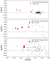 |
Fig. 11. Mean α-element abundance ratios for GCs and field stars in NGC 147, NGC 185 (Vargas et al. 2014), and Fornax (Letarte et al. 2010). |
5. Discussion
The general homogeneity of the α-element abundance patterns among the GCs in our sample, with at most minor differences between GCs in dwarf galaxies and in spirals, was noted in Sect. 4.2. Indeed, the similarity is not restricted to the α-elements, but also extends to most other elements. Three clusters, namely Fornax 4, NGC 6822-SC7, and HM33-B, have significantly different abundance patterns than the rest. From inspection of Figs. 7–10, these three clusters have clearly depleted abundances of Na, Mg, Si, Ca, Ti, Sc, Ni, and possibly also Zn and Eu, compared to the other GCs in our sample. On the other hand, Cr and Mn do not appear to vary in a correlated way with these elements.
A more quantitative way to gain insight into correlations between abundances of different elements is via a Principal Components Analysis (PCA). We used the scikit-learn package (Pedregosa et al. 2011) in Python to carry out a PCA for the abundance measurements [Fe/H], [Na/Fe], [Mg/Fe], [Si/Fe], [Ca/Fe], [Ti/Fe], [Sc/Fe], [Cr/Fe], [Mn/Fe], [Ni/Fe], [Zn/Fe], and [Ba/Fe]. For these elements, measurements are available for all clusters except EXT8 (whose features are very weak owing to the low metallicity) and M 33 H38 (which has a low S/N). Errors on the principal component (PC) vectors were estimated via a Monte-Carlo simulation in which the PCs were recomputed from 1000 random realisations of the dataset. The first four PCs of the dataset are shown in Fig. 12, ordered according to their contributions to the total variance of the dataset. It is clear, and fairly unsurprising, that the first PC, which accounts for more than half of the variance, mainly traces metallicity. The second PC, accounting for 17% of the variance, involves all of the abundance ratios in which the three GCs mentioned above are deficient, also including Zn. This again shows very clearly that variations in the α-elements are strongly correlated with variations in [Na/Fe], [Sc/Fe], [Ni/Fe], and [Zn/Fe].
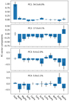 |
Fig. 12. Principal components analysis of the abundance measurements, showing the first four principal components. |
Table 10 lists, for each cluster, the projection of the abundance measurements onto the first four PC vectors. Hence the first column (PC1) indicates metallicity and the second column (PC2) indicates variations in the α-elements and their related elements. We note that PC2 is defined such that a positive increase in this component corresponds to a decrease in the α-element abundances. It is again evident that PC2 has the strongest positive contribution in Fornax 4, HM33-B, and NGC 6822-SC7. The PCA clearly confirms that HM33-B shares similar abundance patterns with Fornax 4 and with NGC 6822-SC7.
Projections of abundance measurement onto principal component vectors.
While the first and second PC have clear astrophysical interpretations, this is less clear for the higher-order PCs. Figure 13 graphically illustrates the data in Table 10 by plotting PC2, PC3, and PC4 as a function of PC1. The three α-deficient GCs are clearly identifiable as outliers in the top panel. PC3 shows a U-shaped variation with PC1, implying a similar U-shaped variation of [Na/Fe] with [Fe/H] and an inverse variation of [Ba/Fe]. This tendency for the most metal-poor and metal-rich clusters to have relatively high [Na/Fe] and relatively low [Ba/Fe] ratios is indeed visible in Figs. 8 and 10. PC4 accounts for less than 6% of the variance, and probably does not trace significant physical variations in the dataset.
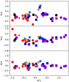 |
Fig. 13. Second, third, and fourth PC as a function of the first PC for each cluster. Symbols are the same as in Fig. 7. |
The relation between [Na/Fe] and the α-elements has previously been discussed in the literature, with conflicting conclusions. Several studies have found significant correlations between [Na/Fe] and [α/Fe] similar to that reported here (Fulbright 2002; I2013), yet no such correlation was found by V2004 in their analysis of a compilation of literature data. Evidently the relationship between Na and the α-elements is complex, as can be appreciated from the fact that relatively metal-rich field stars in dwarf galaxies reach much lower [Na/Fe] values than Galactic stars of comparable metallicities (e.g. Fig. 8).
Similar remarks may be made about the Ni-Na correlation, which has received considerable attention in the literature and is thought to be linked to the production of both elements in Type II SN nucleosynthesis (Nissen & Schuster 1997; Cohen & Huang 2010; Letarte et al. 2010; Lemasle et al. 2014). The two abundance ratios, [Ni/Fe] and [Na/Fe], are also correlated in our dataset though PC2, but cannot here be separated in an unambiguous way from the general correlation of both elements with the α-element abundances.
The identification of the cluster HM33-B in the above analysis is reminiscent of the idea of chemical tagging, which seeks to establish relations between stars or star clusters based on their chemical composition (Freeman & Bland-Hawthorn 2002). Given the small variation in the various abundance ratios at low metallicities, it seems clear that prospects for tagging GCs are most promising for clusters that have metallicities higher than the knee in host galaxies that are sufficiently massive to host GCs, that is, [Fe/H] ≳ −1.5. Similar conclusions were reached in previous work that explored the chemical association of GCs with halo substructure in M 31 (Sakari et al. 2014, 2015) and the Milky Way (Horta et al. 2020).
5.1. Enrichment time scales and IMF
As discussed in the introduction, the integrated light of massive early-type galaxies is usually dominated by old stellar populations with enhanced α-element abundances. When broken down by individual elements the picture becomes more complex. The lighter α-elements (O, Mg) become increasingly enhanced for higher velocity dispersions (i.e. more massive systems), whereas Ca is typically found to be only slightly enhanced relative to scaled-solar composition, or not at all (Conroy et al. 2014; Worthey et al. 2014). These differences reflect differences in nucleosynthetic origin, with the light α-elements being produced predominantly by hydrostatic burning in massive stars, while Ca and Ti are also produced in explosive nucleosynthesis and have significant contributions from type Ia SNe (Woosley & Weaver 1995; McWilliam et al. 2013; Kobayashi et al. 2020). Data for the integrated light of dwarf galaxies are more scarce, but indicate Mg abundances close to scaled-solar values, thus extending the trend of decreasing [α/Fe] ratio with decreasing galaxy mass towards lower masses (Gorgas et al. 1997; Şen et al. 2018).
Abundance measurements for GCs provide a complementary insight into the behaviour of the various abundances at lower metallicities compared to the dominant field star component, and hence at an earlier stage of chemical enrichment (Sect. 4.3). In metal-poor GCs, we find that Ca participates in the general level of α-element enhancement, but at higher metallicities it tends to decrease towards scaled-solar values and thus approaches the behaviour seen in integrated galaxy light. Most of the GCs have metallicities below the knee in the relation of [α/Fe], and at these relatively low metallicities any differences in the mean abundance patterns between dwarf galaxies and the large Local Group spirals are very minor.
In the time-delay model for chemical evolution (Tinsley 1979; Matteucci & Greggio 1986), the abundance ratios at early times, for stars with metallicities below the knee, are expected to depend mainly on the Type II SN yields (see Fig. 10 in Vincenzo et al. 2015 for an illustration). The high degree of similarity of the abundance patterns observed for metal-poor GCs in different environments may therefore not be surprising. However, since the detailed yields do depend on the masses of the Type II SN progenitors (in addition to their metallicity and spin), abundance ratios can, in principle, provide constraints on the shape of the initial mass function (IMF) (Matteucci & Brocato 1990; Nissen et al. 1994; McWilliam 1997; Wyse 1998; Tolstoy et al. 2003). According to chemical evolution models, the α-element abundance patterns of metal-poor stars in the solar neighbourhood are consistent with an early IMF slope similar to, or slightly steeper, than that of the classical Salpeter (1955) IMF (Tsujimoto et al. 1997; Wyse 1998; Hopkins 2018). By way of illustration, Wyse & Gilmore (1992) calculated that a change in IMF slope from −2.3 to −1.1 (where the Salpeter 1955 slope is −2.35) would lead to an increase in [O/Fe] by about 0.4 dex for stars in the Galactic bulge. The details may differ at lower metallicities and for other α-elements, with the effect on Mg, Si, and Ca expected to be about half that on [O/Fe] (Vincenzo et al. 2015). Very roughly, a difference in mean [α/Fe] ratio of about 0.04 dex between dwarf and spiral galaxies (Sect. 4.2) might then correspond to a difference in IMF slope of about 0.2, suggesting that the early IMF in the dwarf galaxies in our sample did not differ substantially from the Salpeter (1955) IMF.
The effects of IMF variations on models for chemical evolution have been explored theoretically for dwarf galaxies (Recchi et al. 2014), including the Sagittarius dSph (Vincenzo et al. 2015), with particular attention to predictions for the Integrated Galactic IMF (IGIMF) theory (Weidner & Kroupa 2005). In this theory, the IMF is coupled to the star formation rate (SFR), with lower SFRs leading to a deficit of high-mass stars and a corresponding lowering of the α-element abundances. The SFRs at early times are generally not well constrained for the dwarf galaxies in our sample. However, the fact that these galaxies were able to form GCs suggests relatively high SFRs. The brightest GCs in each galaxy reach MV ∼ −8 or brighter, corresponding to masses greater than 2.7 × 10⁵ M⊙ (for M/LV = 2 M⊙/LV, ⊙), which translates to SFRs of about 0.8 M⊙ yr−1 or higher in the IGIMF theory (Vincenzo et al. 2015). At such relatively high SFRs, the IGIMF theory predicts only minor differences compared with models that assume classical IMFs. Comparing models with SFRs of 0.5 M⊙ yr−1 and 100 M⊙ yr−1, Recchi et al. (2014) found a difference of only 0.015 dex in the predicted [α/Fe] ratios on the plateau below the knee. These arguments are thus consistent with the similarity of the α-element abundance ratios for GCs in dwarf and spiral galaxies, which suggest that only minor differences in the IMF shape are allowed at low metallicities.
The relatively minor differences in the abundance ratios at low metallicities are in contrast to the more pronounced differences observed at higher metallicities, such as a deficit of hydrostatic elements relative to explosive elements in relatively metal-rich field stars in the Sagittarius dSph (McWilliam et al. 2013). The latter may suggest that the later stages of chemical evolution were characterised by a steeper, more top-light IMF as predicted in the IGIMF theory for the lower SFRs expected at later times (Vincenzo et al. 2015). At lower metallicities, the abundances of stars in Sagittarius are more similar to those observed in the Milky Way halo (and to our GC measurements), consistent with a normal IMF at earlier times (Hansen et al. 2018). It is again worth recalling that some metal-poor GCs also show very low Mg abundances, but linking this to IMF variations is made more difficult by the fact that only some GCs are affected, and by the possibility that Mg is affected by multiple populations.
5.2. Enrichment processes
In Fig. 14 we compare the abundances of Fe, Ba, and Eu, taken as representative tracers of Type Ia SN, s-process, and r-process nucleosynthesis, respectively. In the literature it is customary to plot these elements relative to Mg, taking the latter as a tracer of Type II SN nucleosynthesis (e.g. Skúladóttir & Salvadori 2020). We have here replaced Mg with an error-weighted average of the α-element abundances (Mg, Si, Ca, and Ti) to reduce the uncertainties, and to alleviate the impact of the anomalously low [Mg/Fe] values seen in some GCs. As shown in Fig. 7, this approach is justified by the fairly similar dependencies of the various α-element abundances on metallicity, even though the heavier elements (in particular Ca and Ti) have a more complicated nucleosynthetic history.
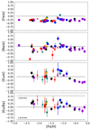 |
Fig. 14. Abundances of heavy elements with respect to the average of the α-elements. Symbols for our measurements as in Fig. 7. |
The top panel in Fig. 14 shows [Fe/α] vs. [Fe/H] and is, of course, equivalent to the mean of the panels in Fig. 7, with the vertical axis inverted, and leads to the same conclusion: for the most part, the GCs are preferentially enriched in the α-elements compared to scaled-solar composition, consistent with enrichment on time scales shorter than those characteristic of Type Ia SNe. Indeed, Fig. 14 suggests the alternative, but equivalent and perhaps more intuitive formulation that the metal-poor GCs are deficient in iron, due to the still ‘missing’ contribution from SN Ia nucleosynthesis. As previously discussed, the main exceptions are Fornax 4, NGC 6822-SC7, and HM33-B. While Fig. 14 shows an average of all four α-elements, the scatter is similar to those of [Ca/Fe] and [Ti/Fe] alone, σ[Fe/α] = 0.09 dex, suggesting that at least part of the dispersion is real.
Similar to [Fe/α], the Ba and Eu abundance ratios, defined with respect to either iron (Fig. 10) or the α-elements (Fig. 14), display no obvious differences depending on the host galaxy. In particular, the apparent enhancement in [Ba/Fe] noted for the M 33 GCs (Sect. 4.2) becomes less clear relative to the α-elements. To be more quantitative, we computed the average [Ba/Fe] for the M 33 GCs and for other GCs in a similar metallicity range (−2 < [Fe/H] < −0.8). We found ⟨[Ba/Fe]⟩M 33 = +0.25 ± 0.03 for the M 33 GCs and ⟨[Ba/Fe]⟩other = +0.21 ± 0.01 for the other GCs, which is only a marginally significant difference. With respect to the α-elements, we instead found ⟨[Ba/α]⟩M 33 = −0.01 ± 0.03 and ⟨[Ba/α]⟩other = 0.00 ± 0.01, which confirms the visual impression from Fig. 14 that no significant difference is present.
As noted in the introduction, the n-capture element abundances are often found to differ significantly between field stars in classical dSph galaxies and the Milky Way. However, at low metallicities, these differences are typically less pronounced (Reichert et al. 2020), in agreement with our results for the GCs. Ultra-faint dwarfs exhibit a larger scatter in the n-capture element abundances that may reflect stochasticity in the enrichment processes dominated by a few rare events (Ji et al. 2016; Marshall et al. 2019; Molero et al. 2021). It is noteworthy that no GC in our sample exhibits the strongly enhanced [Eu/Fe] abundance ratios, up to [Eu/Fe] > 1, recently found for metal-poor stars in the Small and Large Magellanic Cloud (SMC and LMC; Reggiani et al. 2021). These authors suggested that the Eu enhancement in the SMC and LMC stars might result from a more gradual early chemical enrichment history that would have allowed for a more substantial contribution from delayed r-process enrichment due to neutron star mergers. By comparison with our sample, the Magellanic Clouds would appear to have been fairly unique in this respect, even when compared with relatively isolated, irregular galaxies such as NGC 6822 and WLM. A few GCs are consistent with a more moderate Eu enhancement of [Eu/Fe] ≃ 0.6−0.7, as reported for the Gaia Sausage (Aguado et al. 2021) and the Galactic GCs NGC 1261 and NGC 6934 (Koch-Hansen et al. 2021; Marino et al. 2021). Due to the challenging nature of the Eu measurements in the integrated light, independent confirmation of the results for individual clusters would be desirable. However, our measurement of [Eu/Fe] = +0.63 ± 0.04 for the Galactic GC NGC 362 is fairly similar to the literature value of [Eu/Fe] = +0.57 ± 0.02 (Shetrone & Keane 2000; Pritzl et al. 2005).
The [Eu/Ba] ratio, plotted in the lower panel in Fig. 14, is frequently used as an indicator of the importance of r- versus s-process enrichment. The r- and s-process reference ratios are from McWilliam (1997). Our integrated-light measurements mostly lie between the solar system and pure r-process value, but there is a significant scatter. Some GCs, particularly those towards the metal-rich end, even reach sub-solar [Eu/Ba] ratios, implying a more important s-process contribution. Overall, these results are similar to those found for Galactic GCs and field stars in the corresponding metallicity range (McWilliam 1997; Gratton et al. 2004). While Ba is indeed considered a classical tracer of the s-process (according to Bisterzo et al. 2014, about 85% of the Ba in the solar system is attributed to the s-process), Ba production via the r-process becomes increasingly important at early times (Pagel & Tautvaisiene 1997; Cescutti et al. 2006). Europium is, instead, a fairly pure r-process element, with a contribution of only 6% from the s-process in the solar system (Bisterzo et al. 2014). The identification of AGB stars as an important s-process production site is fairly uncontroversial, but s-process elements are also produced in massive stars, so the yields remain not well constrained, as the predictions depend on different parameters in the models, such as rotation, metallicity, and the size of the convective 13C pocket (Cescutti et al. 2006; Prantzos et al. 2018; Limongi & Chieffi 2018; Kobayashi et al. 2020). The details of the r-process are even more uncertain, and it appears increasingly likely that there are at least two r-process sources of which one operates on relatively short time scales (≲108 yr) and is likely linked to massive stars, while the other involves a delay of up to several Gyr and may involve neutron-star mergers (Skúladóttir & Salvadori 2020; Molero et al. 2021). Therefore, the variation in the relative abundances of Ba and Eu as a function of time and metallicity may be expected to be rather more complicated than for the [α/Fe] ratio. Some of the difficulties encountered when modelling the evolution of n-capture elements have been more fully discussed by Tautvaišienė et al. (2021).
Internal variations in the abundances of neutron-capture elements have been observed in NGC 7078 (M 15) and a few other GCs (Roederer 2011), although some cases remain controversial (Cohen 2011). It is reasonable to wonder how this might affect the comparison of n-capture elements in GCs and field stars. In NGC 7078, which is the clearest and best studied case, the member stars fall into two groups with Ba, La, and Eu abundances differing by 0.2−0.4 dex, but both groups have abundance patterns indicative of r-process enrichment. Interestingly, both groups independently show the Na-O anti-correlation that is generally associated with multiple populations in GCs (Sneden et al. 1997; Worley et al. 2013). While the Na spreads in GCs cause clear systematic differences between field stars and mean GC abundances (Fig. 8), internal spreads in n-capture element abundances appear to be relatively rare, and in any case do not make NGC 7078 a significant outlier in the relevant relations. A satisfactory explanation for the spreads in n-capture elements in GCs is even more elusive than for the light element abundance variations. The possibility that r-process self-enrichment in GCs may be caused by neutron-star mergers has been discussed in the literature (e.g. Zevin et al. 2019), but it seems clear from Fig. 10 that such processes do not leave any significant signature in the form of a detectable offset in [Eu/Fe] between GCs and field stars (see also Sakari et al. 2013).
5.3. The extremely metal-poor GC M 31 EXT8
By far the most metal-poor GC in our sample is M 31 EXT8. The spectroscopic observations of this cluster were previously discussed in Larsen et al. (2020) and its CMD was discussed in Larsen et al. (2021).
The metallicity reported here ([Fe/H] = −2.81 ± 0.04) is about 0.1 dex higher than that found in Larsen et al. (2020), mainly due to the application of NLTE corrections (our LTE value is [Fe/H] = −2.88; see Appendix D). As the NLTE corrections also lead to an increase in the metallicites of the other clusters (albeit less so at higher metallicities), the differential change with respect to other GCs in our sample is even smaller. In any case, the slight increase does not change the conclusion that M 31 EXT8 is, by a considerable margin, the most metal-poor GC currently known. It was already noted in previous analysis that the [Mg/Fe] is peculiarly low, while the other α-element abundances are fairly typical of Milky Way field stars at the corresponding metallicity. We note that the [Mg/Fe] measurement in Larsen et al. (2020) was based on the Mg b triplet, while the measurement here is obtained from the weaker Mg I lines that were also used for other clusters in our sample. Nevertheless, we recover the low [Mg/Fe] value previously found.
At the low metallicity of EXT8, the uncertainties on most abundance ratios are relatively large owing to the weakness of the spectral features. There is a suggestion that [Ni/Fe] is somewhat enhanced, but it is not very unusual compared to the Milky Way data when the ∼0.2 dex NLTE correction is accounted for. The [Ba/Fe] value, which has a small uncertainty, is also relatively high, and falls near the upper envelope of [Ba/Fe] values for Galactic halo field stars (Fig. 10). However, [Mg/Fe] remains the most significant outlier in abundance space.
5.4. Outlook: Refining the analysis techniques
While the analysis presented herein has been updated and improved in a variety of ways, it is certainly not definitive. When comparing with model predictions, it is clearly important to eliminate systematic biases in the analysis as much as possible. Even when comparing differentially with other datasets, LTE vs. LTE is not necessarily a like-with-like comparison, owing to the fact that different stellar types and spectral features are affected in different ways by NLTE effects (e.g. Eitner et al. 2019). Here we have applied NLTE corrections for many lines and elements to integrated-light analysis for the first time, and we find that our NLTE abundances for the GCs generally agree well with the corresponding NLTE values for metal-poor Milky Way field stars.
As for individual stars, some elements are more strongly affected by NLTE effects than others. In some cases, application of NLTE corrections can lead to quantitatively different trends with metallicity and different astrophysical implications. A case in point is [Mn/Fe] which displays a strong increasing trend as a function of metallicity in LTE, but remains approximately flat in NLTE. As discussed in Eitner et al. (2020), the flat trend of slightly sub-solar [Mn/Fe] ratios can be reproduced in galactic chemical evolution models in which the Type Ia SN contribution to Mn production is mainly due to sub-Chandrasekhar mass progenitors, with a significant contribution from core collapse SNe as well. In contrast, the steeper trend found in LTE would support Type Ia SN progenitors with near-Chandrasekhar masses.
A similar case to Mn may be Cu. We have not here included NLTE corrections for this element, and our integrated-light analysis (Fig. 10) shows the trend of increasing [Cu/Fe] with metallicity that is also commonly observed in field stars. This is often taken as evidence that Cu behaves as a secondary element, produced by the weak s-process in massive stars (Romano & Matteucci 2007). However, NLTE analyses of Cu tend to find a much shallower trend with metallicity that more closely resembles the behaviour expected for a primary element (Yan et al. 2015; Korotin et al. 2018; Shi et al. 2018). Hence, Cu is another case for which the details of the analysis have important consequences for the astrophysical interpretation, and it might therefore be worthwhile to compute integrated-light NLTE corrections for Cu. Taken together, the abundances of Mn, Zn, and Cu may provide important constraints on Type Ia SN models, in particular the role of the double-detonation scenario in which detonation of a helium-rich surface layer may lead to increased production of these three elements (Lach et al. 2020).
Of course, correction for NLTE effects addresses just one of several approximations made in classical abundance analysis. Another is the assumption that the physical properties of stellar atmospheres are time-independent and depend only on the depth in the atmosphere. In the last decade, significant progress has been made in the computation of 3-dimensional radiation-hydrodynamic models (e.g. Magic et al. 2013) and the resulting stellar spectra, from which it is clear that the effects on the derived abundances can be significant at the level of 0.1 dex or more for some elements (Bergemann et al. 2019; Semenova et al. 2020; Amarsi et al. 2019). One appealing aspect of 3D radiation-hydrodynamic models is that convective motions are explicitly accounted for, which eliminates the mixing length, micro-, and macro-turbulent velocities as free parameters in the analysis.
6. Summary and conclusions
We have presented homogeneous integrated-light abundance measurements for a sample of 45 GCs, including NLTE corrections for several elements. The sample includes clusters in most Local Group galaxies that host GC systems, although it is mostly limited to the brighter half of the GC luminosity function and to relatively compact clusters that are better suited for measurements of their integrated light with single-slit echelle spectrographs. Compared with previously published analyses of a subset of the data, the current analysis has been updated in a number of ways, including a critical revision of the line list, a modified prescription for the assignment of microturbulent velocities, and the use of ATLAS12 model atmospheres with self-consistent chemical composition.
Our main results can be summarised as follows:
-
We have extended the formalism for integrated-light NLTE corrections developed by Eitner et al. (2019) to account for simultaneous fitting of multiple spectral lines.
-
To first order, GCs in different galaxies have very similar abundance patterns. Metal-poor GCs ([Fe/H] ≲ −1.5) have enhanced α-element abundances in all galaxies, and the overall scatter in the α-element abundances is less than 0.1 dex. As in previous studies, we find peculiarly low [Mg/Fe] values for a fraction of the metal-poor GCs.
-
The similarity of the α-element abundances indicates that the GC formed in environments with similar IMFs. There is possibly a small offset of about 0.04 dex between the mean α-element abundances of GCs in dwarf galaxies and in the spirals, which we estimate translates to a variation in the IMF slope of at most 0.2.
-
From a principal components analysis, the α-element abundance variations are found to be correlated with variations in [Na/Fe], [Sc/Fe], [Ni/Fe], and [Zn/Fe]. These correlations are driven mainly by three clusters: Fornax 4, NGC 6822-SC7, and HM33-B. Fornax 4 and NGC 6822-SC7 are the most metal-rich GCs in their respective host galaxies, and the similarity of the abundance patterns of HM33-B to the two other clusters may suggest an accretion origin for HM33-B.
-
The n-capture element abundances are also fairly uniform across our sample. We find no GCs with strongly enhanced r-process signatures, as reported for metal-poor stars in the Magellanic Clouds (Reggiani et al. 2021) and in ultra-faint dwarfs such as Reticulum II (Ji et al. 2016; Roederer et al. 2016).
-
In view of the very similar abundance patterns at low metallicities, and in agreement with previous studies, we conclude that chemical tagging of GCs is likely to work best at metallicities above [Fe/H] ≈ −1.5, where differences between the chemical composition of stellar populations in host dwarf galaxies become more apparent.
-
We measure a line-of-sight velocity dispersion of about 11.7 km s−1 and a corresponding mass-to-light ratio of Mdyn/LV ≃ 2.0 M⊙/LV, ⊙ for the cluster F46 in NGC 2403, consistent with the value expected for a moderately metal-poor old GC.
Beyond the results summarised above, the analysis presented here may also serve as a reference for future studies of larger samples of GCs beyond the Local Group. With the next generation of 30−40 m class telescopes, it will be possible to obtain high S/N spectra for GCs well beyond the Local Group, including in galaxies with rich GC systems (such as the Sombrero galaxy and NGC 5128), of which a substantial fraction will fall in the more metal-rich regime where interesting differences may be expected.
Available at http://www.astro.caltech.edu/~tb/makee/
Acknowledgments
J.S. acknowledges support from the Packard Foundation. A.J.R. was supported by National Science Foundation Grant AST-1616710 and as a Research Corporation for Science Advancement Cottrell Scholar. M.B. is supported through the Lise Meitner grant from the Max Planck Society. We acknowledge support by the Collaborative Research centre SFB 881 (projects A5, A10), Heidelberg University, of the Deutsche Forschungsgemeinschaft (DFG, German Research Foundation). This project has received funding from the European Research Council (ERC) under the European Union’s Horizon 2020 research and innovation programme (Grant agreement No. 949173). Funding for the Sloan Digital Sky Survey (SDSS) has been provided by the Alfred P. Sloan Foundation, the Participating Institutions, the National Aeronautics and Space Administration, the National Science Foundation, the US Department of Energy, the Japanese Monbukagakusho, and the Max Planck Society. The SDSS Website is http://www.sdss.org/. The SDSS is managed by the Astrophysical Research Consortium (ARC) for the Participating Institutions. The Participating Institutions are The University of Chicago, Fermilab, the Institute for Advanced Study, the Japan Participation Group, The Johns Hopkins University, Los Alamos National Laboratory, the Max-Planck-Institute for Astronomy (MPIA), the Max-Planck-Institute for Astrophysics (MPA), New Mexico State University, University of Pittsburgh, Princeton University, the United States Naval Observatory, and the University of Washington. This research has made use of ESASky, developed by the ESAC Science Data Centre (ESDC) team and maintained alongside other ESA science mission’s archives at ESA’s European Space Astronomy Centre (ESAC, Madrid, Spain). Some of the data presented herein were obtained at the W.M. Keck Observatory, which is operated as a scientific partnership among the California Institute of Technology, the University of California and the National Aeronautics and Space Administration. The Observatory was made possible by the generous financial support of the W.M. Keck Foundation. The authors wish to recognize and acknowledge the very significant cultural role and reverence that the summit of Maunakea has always had within the indigenous Hawaiian community. We are most fortunate to have the opportunity to conduct observations from this mountain. We thank A. Wasserman for assistance with the HIRES observations and J. van Eijck for help with selection of lines for NLTE analysis. We are grateful to the anonymous referee for carefully reading the manuscript and delivering a timely report which contained several useful suggestions.
References
- Aguado, D. S., Belokurov, V., Myeong, G. C., et al. 2021, ApJ, 908, L8 [NASA ADS] [CrossRef] [Google Scholar]
- Alam, S., Albareti, F. D., Prieto, C. A., et al. 2015, ApJS, 219, 12 [NASA ADS] [CrossRef] [Google Scholar]
- Alvarez, R., & Plez, B. 1998, A&A, 330, 1109 [NASA ADS] [Google Scholar]
- Alves-Brito, A., Barbuy, B., Zoccali, M., et al. 2006, A&A, 460, 269 [NASA ADS] [CrossRef] [EDP Sciences] [Google Scholar]
- Amarsi, A. M., Nissen, P. E., & Skúladóttir, Á. 2019, A&A, 630, A104 [NASA ADS] [CrossRef] [EDP Sciences] [Google Scholar]
- Andrievsky, S., Bonifacio, P., Caffau, E., et al. 2018, MNRAS, 473, 3377 [NASA ADS] [CrossRef] [Google Scholar]
- Anstee, S. D., & O’Mara, B. J. 1995, MNRAS, 276, 859 [Google Scholar]
- Asplund, M. 2005, ARA&A, 43, 481 [Google Scholar]
- Asplund, M., Grevesse, N., Sauval, A. J., & Scott, P. 2009, ARA&A, 47, 481 [NASA ADS] [CrossRef] [Google Scholar]
- Baade, W. 1944, ApJ, 100, 147 [NASA ADS] [CrossRef] [Google Scholar]
- Barbuy, B., Renzini, A., Ortolani, S., Bica, E., & Guarnieri, M. D. 1999, A&A, 341, 539 [NASA ADS] [Google Scholar]
- Barklem, P. S., Piskunov, N., & O’Mara, B. J. 2000, A&AS, 142, 467 [NASA ADS] [CrossRef] [EDP Sciences] [Google Scholar]
- Barklem, P. S., Belyaev, A. K., Dickinson, A. S., & Gadea, F. X. 2010, A&A, 519, 20 [Google Scholar]
- Barklem, P. S., Osorio, Y., Fursa, D. V., et al. 2017, A&A, 606, 11 [Google Scholar]
- Bastian, N., & Lardo, C. 2018, ARA&A, 56, 83 [Google Scholar]
- Battaglia, G., Tolstoy, E., Helmi, A., et al. 2006, A&A, 459, 423 [NASA ADS] [CrossRef] [EDP Sciences] [Google Scholar]
- Battistini, P., Bonoli, F., Federici, L., Fusi Pecci, F., & Kron, R. G. 1984, A&A, 130, 162 [NASA ADS] [Google Scholar]
- Battistini, P., Bonoli, F., Braccesi, A., et al. 1987, A&AS, 67, 447 [NASA ADS] [Google Scholar]
- Beasley, M. A., Brodie, J. P., Strader, J., et al. 2005, AJ, 129, 1412 [NASA ADS] [CrossRef] [Google Scholar]
- Beasley, M. A., Bridges, T., Peng, E., et al. 2008, MNRAS, 386, 1443 [NASA ADS] [CrossRef] [Google Scholar]
- Beasley, M. A., San Roman, I., Gallart, C., Sarajedini, A., & Aparicio, A. 2015, MNRAS, 451, 3400 [Google Scholar]
- Belokurov, V., Erkal, D., Evans, N. W., Koposov, S. E., & Deason, A. J. 2018, MNRAS, 478, 611 [Google Scholar]
- Bensby, T., Feltzing, S., Gould, A., et al. 2017, A&A, 605, A89 [NASA ADS] [CrossRef] [EDP Sciences] [Google Scholar]
- Bergemann, M., & Cescutti, G. 2010, A&A, 522, A9 [NASA ADS] [CrossRef] [EDP Sciences] [Google Scholar]
- Bergemann, M., Lind, K., Collet, R., & Asplund, M. 2011, J. Phys.: Conf. Ser., 328, 012002 [NASA ADS] [CrossRef] [Google Scholar]
- Bergemann, M., Lind, K., Collet, R., Magic, Z., & Asplund, M. 2012, MNRAS, 427, 27 [Google Scholar]
- Bergemann, M., Collet, R., Amarsi, A. M., et al. 2017a, ApJ, 847, 15 [NASA ADS] [CrossRef] [Google Scholar]
- Bergemann, M., Collet, R., Schönrich, R., et al. 2017b, ApJ, 847, 16 [Google Scholar]
- Bergemann, M., Sesar, B., Cohen, J. G., et al. 2018, Nature, 555, 334 [Google Scholar]
- Bergemann, M., Gallagher, A. J., Eitner, P., et al. 2019, A&A, 631, A80 [NASA ADS] [CrossRef] [EDP Sciences] [Google Scholar]
- Bergemann, M., Hoppe, R., Semenova, E., et al. 2021, MNRAS, 508, 2236 [NASA ADS] [CrossRef] [Google Scholar]
- Bisterzo, S., Travaglio, C., Gallino, R., Wiescher, M., & Käppeler, F. 2014, ApJ, 787, 10 [NASA ADS] [CrossRef] [Google Scholar]
- Boeche, C., & Grebel, E. K. 2016, A&A, 587, A2 [NASA ADS] [CrossRef] [EDP Sciences] [Google Scholar]
- Bohlin, R. C. 2016, AJ, 152, 60 [NASA ADS] [CrossRef] [Google Scholar]
- Bonifacio, P., Spite, M., Cayrel, R., et al. 2009, A&A, 501, 519 [NASA ADS] [CrossRef] [EDP Sciences] [Google Scholar]
- Brewer, J. M., Fischer, D. A., Basu, S., Valenti, J. A., & Piskunov, N. 2015, ApJ, 805, 126 [Google Scholar]
- Brodie, J. P., & Huchra, J. P. 1990, ApJ, 362, 503 [NASA ADS] [CrossRef] [Google Scholar]
- Brodie, J. P., & Huchra, J. P. 1991, ApJ, 379, 157 [NASA ADS] [CrossRef] [Google Scholar]
- Brodie, J. P., & Strader, J. 2006, ARA&A, 44, 193 [Google Scholar]
- Brooke, J. S. A., Ram, R. S., Western, C. M., et al. 2014, ApJS, 210, 23 [NASA ADS] [CrossRef] [Google Scholar]
- Brown, A. G. A. 2021, ARA&A, 59, 59 [NASA ADS] [CrossRef] [Google Scholar]
- Brown, A. G. A., Vallenari, A., Prusti, T., et al. 2021, A&A, 649, A1 [NASA ADS] [CrossRef] [EDP Sciences] [Google Scholar]
- Bruzual, G., & Charlot, S. 2003, MNRAS, 344, 1000 [NASA ADS] [CrossRef] [Google Scholar]
- Buck, T. 2020, MNRAS, 491, 5435 [NASA ADS] [CrossRef] [Google Scholar]
- Buck, T., Rybizki, J., Buder, S., et al. 2021, MNRAS, 508, 3365 [NASA ADS] [CrossRef] [Google Scholar]
- Buder, S., Sharma, S., Kos, J., et al. 2021, MNRAS, 506, 150 [NASA ADS] [CrossRef] [Google Scholar]
- Buonanno, R., Corsi, C. E., Castellani, M., et al. 1999, AJ, 118, 1671 [NASA ADS] [CrossRef] [Google Scholar]
- Burbidge, E., Burbidge, G., Fowler, W., & Hoyle, F. 1957, Rev. Mod. Phys., 29, 547 [NASA ADS] [CrossRef] [Google Scholar]
- Butler, R. P., Vogt, S. S., Laughlin, G., et al. 2017, AJ, 153, 208 [Google Scholar]
- Caldwell, N., Schiavon, R., Morrison, H., Rose, J. A., & Harding, P. 2011, AJ, 141, 61 [NASA ADS] [CrossRef] [Google Scholar]
- Carlsson, M. 1986, Upps. Astron. Obs. Rep., 33, 2 [Google Scholar]
- Carretta, E., & Gratton, R. G. 1997, A&AS, 121, 95 [NASA ADS] [CrossRef] [EDP Sciences] [Google Scholar]
- Carretta, E., Bragaglia, A., Gratton, R., & Lucatello, S. 2009a, A&A, 505, 139 [NASA ADS] [CrossRef] [EDP Sciences] [Google Scholar]
- Carretta, E., Bragaglia, A., Gratton, R. G., et al. 2009b, A&A, 505, 117 [NASA ADS] [CrossRef] [EDP Sciences] [Google Scholar]
- Castelli, F. 2005, Mem. Soc. Astron. It. Suppl., 8, 44 [Google Scholar]
- Castelli, F., & Hubrig, S. 2004, A&A, 425, 263 [NASA ADS] [CrossRef] [EDP Sciences] [Google Scholar]
- Castelli, F., & Kurucz, R. L. 2003, in Modelling of Stellar Atmospheres, Proc. of the 210th Symposium of the IAU, eds. N. Piskunov, W. W. Weiss, & D. F. Gray, 210, 20 [NASA ADS] [Google Scholar]
- Cayrel, R. 1988, in The Impact of Very High S/N Spectroscopy on Stellar Physics, eds. G. Cayrel de Strobel, & M. Spite (Dordrecht: Kluwer Academic Publishers), IAU Symp., 132, 345 [Google Scholar]
- Cenarro, A. J., Beasley, M. A., Strader, J., Brodie, J. P., & Forbes, D. A. 2007, AJ, 134, 391 [NASA ADS] [CrossRef] [Google Scholar]
- Černiauskas, A., Kučinskas, A., Klevas, J., et al. 2018, A&A, 616, A142 [NASA ADS] [CrossRef] [EDP Sciences] [Google Scholar]
- Cescutti, G., François, P., Matteucci, F., Cayrel, R., & Spite, M. 2006, A&A, 448, 557 [NASA ADS] [CrossRef] [EDP Sciences] [Google Scholar]
- Chandar, R., Bianchi, L., & Ford, H. C. 1999, ApJS, 122, 431 [NASA ADS] [CrossRef] [Google Scholar]
- Christian, C. A., & Schommer, R. A. 1982, ApJS, 49, 405 [NASA ADS] [CrossRef] [Google Scholar]
- Cohen, J. G. 1978, ApJ, 223, 487 [Google Scholar]
- Cohen, J. G. 2011, ApJ, 740, L38 [NASA ADS] [CrossRef] [Google Scholar]
- Cohen, J. G., & Blakeslee, J. P. 1998, AJ, 115, 2356 [NASA ADS] [CrossRef] [Google Scholar]
- Cohen, J. G., & Huang, W. 2009, ApJ, 701, 1053 [NASA ADS] [CrossRef] [Google Scholar]
- Cohen, J. G., & Huang, W. 2010, ApJ, 719, 931 [NASA ADS] [CrossRef] [Google Scholar]
- Cohen, J. G., Briley, M. M., & Stetson, P. B. 2002, AJ, 123, 2525 [NASA ADS] [CrossRef] [Google Scholar]
- Colucci, J., & Bernstein, R. 2011, EAS Pub. Ser., 48, 275 [NASA ADS] [CrossRef] [EDP Sciences] [Google Scholar]
- Colucci, J. E., Bernstein, R. A., Cameron, S., McWilliam, A., & Cohen, J. G. 2009, ApJ, 704, 385 [NASA ADS] [CrossRef] [Google Scholar]
- Colucci, J. E., Duran, M. F., Bernstein, R. A., & McWilliam, A. 2013, ApJ, 773, L36 [NASA ADS] [CrossRef] [Google Scholar]
- Colucci, J. E., Bernstein, R. A., & Cohen, J. G. 2014, ApJ, 797, 116 [NASA ADS] [CrossRef] [Google Scholar]
- Colucci, J. E., Bernstein, R. A., & McWilliam, A. 2017, ApJ, 834, 105 [NASA ADS] [CrossRef] [Google Scholar]
- Conroy, C., & van Dokkum, P. G. 2012, ApJ, 760, 71 [Google Scholar]
- Conroy, C., Graves, G. J., & van Dokkum, P. G. 2014, ApJ, 780, 33 [Google Scholar]
- Conroy, C., Villaume, A., van Dokkum, P. G., & Lind, K. 2018, ApJ, 854, 139 [Google Scholar]
- Cook, B. A., Conroy, C., Pillepich, A., et al. 2016, ApJ, 833, 158 [NASA ADS] [CrossRef] [Google Scholar]
- Cooper, A. P., Cole, S., Frenk, C. S., et al. 2010, MNRAS, 406, 744 [Google Scholar]
- Cordoni, G., Da Costa, G. S., Yong, D., et al. 2021, MNRAS, 503, 2539 [NASA ADS] [CrossRef] [Google Scholar]
- Cox, A. N. 2000, Allen’s Astrophysical Quantities, 4th edn. (New York: AIP Press) [Google Scholar]
- Da Costa, G. S., & Mould, J. R. 1988, ApJ, 334, 159 [NASA ADS] [CrossRef] [Google Scholar]
- da Silveira, C. R., Barbuy, B., Friaça, A. C. S., et al. 2018, A&A, 614, A149 [NASA ADS] [CrossRef] [EDP Sciences] [Google Scholar]
- Davison, T. A., Norris, M. A., Leaman, R., et al. 2021, MNRAS, 507, 3089 [NASA ADS] [CrossRef] [Google Scholar]
- Dekker, H., D’Odorico, S., Kaufer, A., Delabre, B., & Kotzlowski, H. 2000, Proc. SPIE, 4008, 534 [Google Scholar]
- Dotter, A., Chaboyer, B., Jevremović, D., et al. 2007, AJ, 134, 376 [NASA ADS] [CrossRef] [Google Scholar]
- Drawin, H.-W., & Felenbok, P. 1965, Data for Plasmas in Local Thermodynamic Equilibrium (Paris: Gauthier-Villars) [Google Scholar]
- Dubath, P., Meylan, G., & Mayor, M. 1992, ApJ, 400, 510 [NASA ADS] [CrossRef] [Google Scholar]
- Dutra-Ferreira, L., Pasquini, L., Smiljanic, R., de Mello, G. F. P., & Steffen, M. 2016, A&A, 585, A75 [NASA ADS] [CrossRef] [EDP Sciences] [Google Scholar]
- Eggen, O. J., Lynden-Bell, D., & Sandage, A. R. 1962, ApJ, 136, 748 [NASA ADS] [CrossRef] [Google Scholar]
- Eitner, P., Bergemann, M., & Larsen, S. S. 2019, A&A, 627, A40 [NASA ADS] [CrossRef] [EDP Sciences] [Google Scholar]
- Eitner, P., Bergemann, M., Hansen, C., et al. 2020, A&A, 635, A38 [NASA ADS] [CrossRef] [EDP Sciences] [Google Scholar]
- Escala, I., Kirby, E. N., Gilbert, K. M., Cunningham, E. C., & Wojno, J. 2019, ApJ, 878, 42 [NASA ADS] [CrossRef] [Google Scholar]
- Escala, I., Gilbert, K. M., Kirby, E. N., et al. 2020, ApJ, 889, 177 [Google Scholar]
- Forbes, D. A. 2020, MNRAS, 493, 847 [Google Scholar]
- Forte, J. C., Strom, S. E., & Strom, K. M. 1981, ApJ, 245, L9 [NASA ADS] [CrossRef] [Google Scholar]
- Frebel, A. 2010, Astron. Nachr., 331, 474 [NASA ADS] [CrossRef] [Google Scholar]
- Freedman, W. L., & Madore, B. F. 1988, ApJ, 332, L63 [NASA ADS] [CrossRef] [Google Scholar]
- Freeman, K., & Bland-Hawthorn, J. 2002, ARA&A, 40, 487 [Google Scholar]
- Fulbright, J. P. 2002, AJ, 123, 404 [NASA ADS] [CrossRef] [Google Scholar]
- Fulbright, J. P., McWilliam, A., & Rich, R. M. 2006, ApJ, 636, 821 [Google Scholar]
- Furenlid, I. 1988, in The Impact of Very High S/N Spectroscopy on Stellar Physics, eds. G. Cayrel de Strobel, & M. Spite (Dordrecht: Kluwer Academic Publishers), IAU Symp., 132, 435 [NASA ADS] [CrossRef] [Google Scholar]
- Gallagher, A. J., Bergemann, M., Collet, R., et al. 2020, A&A, 634, A55 [NASA ADS] [CrossRef] [EDP Sciences] [Google Scholar]
- Galleti, S., Federici, L., Bellazzini, M., Pecci, F. F., & Macrina, S. 2004, A&A, 416, 917 [NASA ADS] [CrossRef] [EDP Sciences] [Google Scholar]
- Gehren, T., Liang, Y. C., Shi, J. R., Zhang, H. W., & Zhao, G. 2004, A&A, 413, 1045 [NASA ADS] [CrossRef] [EDP Sciences] [Google Scholar]
- Gehren, T., Shi, J. R., Zhang, H. W., Zhao, G., & Korn, A. J. 2006, A&A, 451, 1065 [NASA ADS] [CrossRef] [EDP Sciences] [Google Scholar]
- Genel, S., Vogelsberger, M., Springel, V., et al. 2014, MNRAS, 445, 175 [Google Scholar]
- Gieren, W., Górski, M., Pietrzyński, G., et al. 2013, ApJ, 773, 69 [Google Scholar]
- Gilbert, K. M., Wojno, J., Kirby, E. N., et al. 2020, AJ, 160, 41 [NASA ADS] [CrossRef] [Google Scholar]
- Gilmore, G., & Wyse, R. F. G. 1998, AJ, 116, 748 [NASA ADS] [CrossRef] [Google Scholar]
- Gorgas, J., Pedraz, S., Guzman, R., Cardiel, N., & Gonzalez, J. J. 1997, ApJ, 481, L19 [NASA ADS] [CrossRef] [Google Scholar]
- Gratton, R. G., & Sneden, C. 1987, A&A, 178, 179 [NASA ADS] [Google Scholar]
- Gratton, R. G., Carretta, E., Eriksson, K., & Gustafsson, B. 1999, A&A, 350, 955 [NASA ADS] [Google Scholar]
- Gratton, R. G., Sneden, C., Carretta, E., & Bragaglia, A. 2000, A&A, 354, 169 [NASA ADS] [Google Scholar]
- Gratton, R. G., Carretta, E., Claudi, R., Lucatello, S., & Barbieri, M. 2003, A&A, 404, 187 [NASA ADS] [CrossRef] [EDP Sciences] [Google Scholar]
- Gratton, R., Sneden, C., & Carretta, E. 2004, ARA&A, 42, 385 [Google Scholar]
- Gratton, R. G., Carretta, E., & Bragaglia, A. 2012, A&ARv, 20, 1 [CrossRef] [Google Scholar]
- Gratton, R., Bragaglia, A., Carretta, E., et al. 2019, A&ARv, 27, 8 [Google Scholar]
- Graves, G. J., & Schiavon, R. P. 2008, ApJS, 177, 446 [NASA ADS] [CrossRef] [Google Scholar]
- Greener, M. J., Merrifield, M., Aragón-Salamanca, A., et al. 2021, MNRAS, 502, L95 [Google Scholar]
- Grevesse, N., & Sauval, A. J. 1998, Space Sci. Rev., 85, 161 [Google Scholar]
- Grumer, J., & Barklem, P. S. 2020, A&A, 637, A28 [NASA ADS] [CrossRef] [EDP Sciences] [Google Scholar]
- Gustafsson, B., Edvardsson, B., Eriksson, K., et al. 2008, A&A, 486, 951 [NASA ADS] [CrossRef] [EDP Sciences] [Google Scholar]
- Hansen, C. J., El-Souri, M., Monaco, L., et al. 2018, ApJ, 855, 83 [NASA ADS] [CrossRef] [Google Scholar]
- Hardy, E. 2002, in Extragalactic Star Clusters, eds. D. Geisler, E. K. Grebel, & D. Minniti (San Francisco: ASP), IAU Symp., 207, 62 [NASA ADS] [Google Scholar]
- Harris, W. E. 1996, AJ, 112, 1487 [Google Scholar]
- Harris, W. E., Harris, G. L. H., Layden, A. C., & Wehner, E. M. H. 2007, ApJ, 666, 903 [NASA ADS] [CrossRef] [Google Scholar]
- Hasselquist, S., Shetrone, M., Smith, V., et al. 2017, ApJ, 845, 162 [Google Scholar]
- Helmi, A., Babusiaux, C., Koppelman, H. H., et al. 2018, Nature, 563, 85 [Google Scholar]
- Hendricks, B., Koch, A., Walker, M., et al. 2014, A&A, 572, A82 [NASA ADS] [CrossRef] [EDP Sciences] [Google Scholar]
- Hendricks, B., Boeche, C., Johnson, C. I., et al. 2016, A&A, 585, A86 [NASA ADS] [CrossRef] [EDP Sciences] [Google Scholar]
- Herbig, G. H. 1975, ApJ, 196, 129 [NASA ADS] [CrossRef] [Google Scholar]
- Hernandez, S., Larsen, S., Trager, S., Kaper, L., & Groot, P. 2018, MNRAS, 476, 5189 [NASA ADS] [CrossRef] [Google Scholar]
- Herschel, J. F. W. 1847, Results of Astronomical Observations made During the Years 1834, 5, 6, 7, 8, at the Cape of Good Hope; being the Completion of a Telescopic Survey of the Whole Surface of the Visible Heavens, Commenced in 1825 (London: Smith, Elder and Co.) [Google Scholar]
- Hidalgo, S. L., Pietrinferni, A., Cassisi, S., et al. 2018, ApJ, 856, 125 [Google Scholar]
- Hiltner, W. A. 1960, ApJ, 131, 163 [NASA ADS] [CrossRef] [Google Scholar]
- Hodge, P. W. 1961, AJ, 66, 83 [NASA ADS] [CrossRef] [Google Scholar]
- Hodge, P. W., Dolphin, A. E., Smith, T. R., & Mateo, M. 1999, ApJ, 521, 577 [NASA ADS] [CrossRef] [Google Scholar]
- Hopkins, A. M. 2018, PASA, 35, e039 [NASA ADS] [CrossRef] [Google Scholar]
- Horta, D., Schiavon, R. P., Mackereth, J. T., et al. 2020, MNRAS, 493, 3363 [NASA ADS] [CrossRef] [Google Scholar]
- Hubble, E. 1932, ApJ, 76, 44 [NASA ADS] [CrossRef] [Google Scholar]
- Hubble, E. P. 1925, ApJ, 62, 409 [NASA ADS] [CrossRef] [Google Scholar]
- Humason, M. L., Mayall, N. U., & Sandage, A. R. 1956, AJ, 61, 97 [CrossRef] [Google Scholar]
- Huxor, A., Ferguson, A. M. N., Barker, M. K., et al. 2009, ApJ, 698, L77 [NASA ADS] [CrossRef] [Google Scholar]
- Huxor, A., Ferguson, A., Veljanoski, J., Mackey, D., & Tanvir, N. 2013, MNRAS, 429, 1039 [NASA ADS] [CrossRef] [Google Scholar]
- Huxor, A. P., Mackey, A. D., Ferguson, A. M. N., et al. 2014, MNRAS, 442, 2165 [Google Scholar]
- Hwang, N., Lee, M. G., Lee, J. C., et al. 2011, ApJ, 738, 58 [NASA ADS] [CrossRef] [Google Scholar]
- Ibata, R. A., Gilmore, G., & Irwin, M. J. 1994, Nature, 370, 194 [Google Scholar]
- Ibata, R. A., Lewis, G. F., McConnachie, A. W., et al. 2014, ApJ, 780, 128 [Google Scholar]
- Igenbergs, K., Schweinzer, J., Bray, I., Bridi, D., & Aumayr, F. 2008, At. Data Nucl. Data Tables, 94, 981 [NASA ADS] [CrossRef] [Google Scholar]
- Irwin, A. W. 1981, ApJS, 45, 621 [NASA ADS] [CrossRef] [Google Scholar]
- Ishigaki, M. N., Aoki, W., & Chiba, M. 2013, ApJ, 771, 67 [NASA ADS] [CrossRef] [Google Scholar]
- Jefferies, J. T. 1968, Spectral Line Formation (Waltham, Massachusetts: Blaisdell Publishing Company) [Google Scholar]
- Ji, A. P., Frebel, A., Chiti, A., & Simon, J. D. 2016, Nature, 531, 610 [NASA ADS] [CrossRef] [Google Scholar]
- Jofré, P., Heiter, U., & Soubiran, C. 2019, ARA&A, 57, 571 [Google Scholar]
- Johnson, C. I., Rich, R. M., Kobayashi, C., & Fulbright, J. P. 2012, ApJ, 749, 175 [NASA ADS] [CrossRef] [Google Scholar]
- Keenan, P. C., & McNeil, R. C. 1989, ApJS, 71, 245 [Google Scholar]
- Kinman, T. D. 1959, MNRAS, 119, 538 [NASA ADS] [CrossRef] [Google Scholar]
- Kirby, E. N., Lanfranchi, G. A., Simon, J. D., Cohen, J. G., & Guhathakurta, P. 2011, ApJ, 727, 78 [Google Scholar]
- Kirby, E. N., Xie, J. L., Guo, R., et al. 2019, ApJ, 881, 45 [NASA ADS] [CrossRef] [Google Scholar]
- Kobayashi, C., Haynes, C. J., & Vincenzo, F. 2019, in Why Galaxies Care About AGB Stars: A Continuing Challenge through Cosmic Time (Cambridge: Cambridge University Press), IAU Symp., 343, 247 [Google Scholar]
- Kobayashi, C., Karakas, A. I., & Lugaro, M. 2020, ApJ, 900, 179 [Google Scholar]
- Koch, A., & McWilliam, A. 2008, AJ, 135, 1551 [NASA ADS] [CrossRef] [Google Scholar]
- Koch-Hansen, A. J., Hansen, C. J., & McWilliam, A. 2021, A&A, 653, A2 [NASA ADS] [CrossRef] [EDP Sciences] [Google Scholar]
- Kondo, S., Fukue, K., Matsunaga, N., et al. 2019, ApJ, 875, 129 [NASA ADS] [CrossRef] [Google Scholar]
- Korotin, S. A., Andrievsky, S. M., & Zhukova, A. V. 2018, MNRAS, 480, 965 [NASA ADS] [CrossRef] [Google Scholar]
- Kovalev, M., Bergemann, M., Ting, Y. S., & Rix, H. W. 2019, A&A, 628, 54 [Google Scholar]
- Kramida, A., Ralchenko, Y., & Reader, J. 2013, NIST Atomic Spectra Database, http://physics.nist.gov/asd [Google Scholar]
- Kriek, M., Price, S. H., Conroy, C., et al. 2019, ApJ, 880, L31 [NASA ADS] [CrossRef] [Google Scholar]
- Kron, G. E., & Mayall, N. U. 1960, AJ, 65, 581 [NASA ADS] [CrossRef] [Google Scholar]
- Kroupa, P. 2001, MNRAS, 322, 231 [NASA ADS] [CrossRef] [Google Scholar]
- Kruijssen, J. M. D., Pfeffer, J. L., Chevance, M., et al. 2020, MNRAS, 498, 2472 [NASA ADS] [CrossRef] [Google Scholar]
- Kuntschner, H. 2000, MNRAS, 315, 184 [NASA ADS] [CrossRef] [Google Scholar]
- Kupka, F., Piskunov, N., Ryabchikova, T. A., Stempels, H. C., & Weiss, W. W. 1999, A&AS, 138, 119 [NASA ADS] [CrossRef] [EDP Sciences] [Google Scholar]
- Kurucz, R. L. 1970, Atlas: A Computer Program for Calculating Model Stellar Atmospheres (Smithsonian Astrophysical Observatory), http://kurucz.harvard.edu/papers/sao309/saospecialreport309.pdf [Google Scholar]
- Kurucz, R. L. 2005, Mem. Soc. Astron. It. Suppl., 8, 14 [Google Scholar]
- Kurucz, R. L., & Avrett, E. H. 1981, Solar Spectrum Synthesis. I. A Sample Atlas from 224 to 300 nm (Smithsonian Astrophysical Observatory), http://kurucz.harvard.edu/papers/sao391/saosr391.pdf [Google Scholar]
- Kurucz, R. L., Furenlid, I., Brault, J., & Testerman, L. 1984, Solar Flux Atlas from 296 to 1300 nm (Sunspot: National Solar Observatory) [Google Scholar]
- La Barbera, F., Vazdekis, A., Ferreras, I., et al. 2017, MNRAS, 464, 3597 [Google Scholar]
- Lach, F., Röpke, F. K., Seitenzahl, I. R., et al. 2020, A&A, 644, A118 [NASA ADS] [CrossRef] [EDP Sciences] [Google Scholar]
- Lamers, H. J. G. L. M., Kruijssen, J. M. D., Bastian, N., et al. 2017, A&A, 606, A85 [NASA ADS] [CrossRef] [EDP Sciences] [Google Scholar]
- Lapenna, E., Mucciarelli, A., Lanzoni, B., et al. 2014, ApJ, 797, 124 [NASA ADS] [CrossRef] [Google Scholar]
- Lardo, C., Pancino, E., Mucciarelli, A., & Milone, A. P. 2012, A&A, 548, A107 [NASA ADS] [CrossRef] [EDP Sciences] [Google Scholar]
- Larsen, S. 2020, https://doi.org/10.5281/zenodo.4036092 [Google Scholar]
- Larsen, S., Brodie, J., Beasley, M., & Forbes, D. 2002a, AJ, 124, 828 [NASA ADS] [CrossRef] [Google Scholar]
- Larsen, S. S., Brodie, J. P., Sarajedini, A., & Huchra, J. P. 2002b, AJ, 124, 2615 [NASA ADS] [CrossRef] [Google Scholar]
- Larsen, S. S., Brodie, J. P., & Strader, J. 2012, A&A, 546, A53 [NASA ADS] [CrossRef] [EDP Sciences] [Google Scholar]
- Larsen, S. S., Brodie, J. P., Forbes, D. A., & Strader, J. 2014, A&A, 565, A98 [NASA ADS] [CrossRef] [EDP Sciences] [Google Scholar]
- Larsen, S. S., Brodie, J. P., & Strader, J. 2017, A&A, 601, A96 [NASA ADS] [CrossRef] [EDP Sciences] [Google Scholar]
- Larsen, S. S., Brodie, J. P., Wasserman, A., & Strader, J. 2018a, A&A, 613, A56 [NASA ADS] [CrossRef] [EDP Sciences] [Google Scholar]
- Larsen, S. S., Pugliese, G., & Brodie, J. P. 2018b, A&A, 617, A119 [NASA ADS] [CrossRef] [EDP Sciences] [Google Scholar]
- Larsen, S. S., Romanowsky, A. J., Brodie, J. P., & Wasserman, A. 2020, Science, 370, 970 [NASA ADS] [CrossRef] [Google Scholar]
- Larsen, S. S., Romanowsky, A. J., & Brodie, J. P. 2021, A&A, 651, A102 [NASA ADS] [CrossRef] [EDP Sciences] [Google Scholar]
- Laverick, M., Lobel, A., Royer, P., et al. 2019, A&A, 624, A60 [NASA ADS] [CrossRef] [EDP Sciences] [Google Scholar]
- Leaman, R., Venn, K. A., Brooks, A. M., et al. 2013, ApJ, 767, 131 [NASA ADS] [CrossRef] [Google Scholar]
- Lemasle, B., de Boer, T., Hill, V., et al. 2014, A&A, 572, A88 [NASA ADS] [CrossRef] [EDP Sciences] [Google Scholar]
- Letarte, B., Hill, V., Jablonka, P., et al. 2006, A&A, 453, 547 [NASA ADS] [CrossRef] [EDP Sciences] [Google Scholar]
- Letarte, B., Hill, V., Tolstoy, E., et al. 2010, A&A, 523, A17 [NASA ADS] [CrossRef] [EDP Sciences] [Google Scholar]
- Limongi, M., & Chieffi, A. 2018, ApJS, 237, 13 [NASA ADS] [CrossRef] [Google Scholar]
- Lind, K., Asplund, M., Barklem, P. S., & Belyaev, A. K. 2011, A&A, 528, A103 [NASA ADS] [CrossRef] [EDP Sciences] [Google Scholar]
- Liu, Y., Romero-Romero, E., Garand, D., et al. 2019, Spectrochim. Acta Part B: At. Spectr., 158, 105640 [NASA ADS] [CrossRef] [Google Scholar]
- Lodders, K. 2003, ApJ, 591, 1220 [Google Scholar]
- Luck, R. E., & Bond, H. E. 1981, ApJ, 244, 919 [NASA ADS] [CrossRef] [Google Scholar]
- Mackereth, J. T., Schiavon, R. P., Pfeffer, J., et al. 2019, MNRAS, 482, 3426 [Google Scholar]
- Mackey, A. D., & Gilmore, G. F. 2003, MNRAS, 340, 175 [Google Scholar]
- Mackey, A. D., Ferguson, A. M., Huxor, A. P., et al. 2019, MNRAS, 484, 1756 [NASA ADS] [CrossRef] [Google Scholar]
- Magic, Z., Collet, R., Asplund, M., et al. 2013, A&A, 557, A26 [NASA ADS] [CrossRef] [EDP Sciences] [Google Scholar]
- Malhan, K., Ibata, R. A., & Martin, N. F. 2018, MNRAS, 481, 3442 [Google Scholar]
- Marino, A. F., Milone, A. P., Renzini, A., et al. 2021, ApJ, 923, 22 [CrossRef] [Google Scholar]
- Marshall, J. L., Hansen, T., Simon, J. D., et al. 2019, ApJ, 882, 177 [NASA ADS] [CrossRef] [Google Scholar]
- Martell, S. L., Smith, G. H., & Briley, M. M. 2008, AJ, 136, 2522 [NASA ADS] [CrossRef] [Google Scholar]
- Martocchia, S., Dalessandro, E., Salaris, M., Larsen, S., & Rejkuba, M. 2020, MNRAS, 495, 4518 [NASA ADS] [CrossRef] [Google Scholar]
- Martocchia, S., Lardo, C., Rejkuba, M., et al. 2021, MNRAS, 505, 5389 [NASA ADS] [CrossRef] [Google Scholar]
- Mashonkina, L., Korn, A. J., & Przybilla, N. 2007, A&A, 461, 261 [NASA ADS] [CrossRef] [EDP Sciences] [Google Scholar]
- Mashonkina, L., Jablonka, P., Pakhomov, Y., Sitnova, T., & North, P. 2017a, A&A, 604, A129 [NASA ADS] [CrossRef] [EDP Sciences] [Google Scholar]
- Mashonkina, L., Jablonka, P., Sitnova, T., Pakhomov, Y., & North, P. 2017b, A&A, 608, 89 [Google Scholar]
- Mashonkina, L. I., Neretina, M. D., Sitnova, T. M., & Pakhomov, Y. V. 2019, Astron. Rep., 63, 726 [NASA ADS] [CrossRef] [Google Scholar]
- Masseron, T. 2006, PhD Thesis, Observatoire de Paris [Google Scholar]
- Masseron, T., Plez, B., Van Eck, S., et al. 2014, A&A, 571, A47 [NASA ADS] [CrossRef] [EDP Sciences] [Google Scholar]
- Matsuno, T., Aoki, W., Casagrande, L., et al. 2021a, ApJ, 912, 72 [NASA ADS] [CrossRef] [Google Scholar]
- Matsuno, T., Hirai, Y., Tarumi, Y., et al. 2021b, A&A, 650, A110 [NASA ADS] [CrossRef] [EDP Sciences] [Google Scholar]
- Matteucci, F., & Brocato, E. 1990, ApJ, 365, 539 [CrossRef] [Google Scholar]
- Matteucci, F., & Greggio, L. 1986, A&A, 154, 279 [NASA ADS] [Google Scholar]
- Mayall, N. U. 1946, ApJ, 104, 290 [Google Scholar]
- McConnachie, A. W., Ibata, R., Martin, N., et al. 2018, ApJ, 868, 55 [Google Scholar]
- McWilliam, A. 1997, ARA&A, 35, 503 [NASA ADS] [CrossRef] [Google Scholar]
- McWilliam, A. 1998, AJ, 115, 1640 [NASA ADS] [CrossRef] [Google Scholar]
- McWilliam, A., & Bernstein, R. A. 2008, ApJ, 684, 326 [NASA ADS] [CrossRef] [Google Scholar]
- McWilliam, A., Rich, R. M., & Smecker-Hane, T. A. 2003, ApJ, 592, L21 [NASA ADS] [CrossRef] [Google Scholar]
- McWilliam, A., Wallerstein, G., & Mottini, M. 2013, ApJ, 778, 149 [NASA ADS] [CrossRef] [Google Scholar]
- Melnick, J., & D’Odorico, S. 1978, A&AS, 34, 249 [NASA ADS] [Google Scholar]
- Mihalas, D. 1970, Stellar Atmospheres (San Francisco: W.H. Freeman) [Google Scholar]
- Minelli, A., Mucciarelli, A., Massari, D., et al. 2021, ApJ, 918, L32 [NASA ADS] [CrossRef] [Google Scholar]
- Mishenina, T., Pignatari, M., Cot’e, B., et al. 2017, MNRAS, 469, 4378 [NASA ADS] [CrossRef] [Google Scholar]
- Molero, M., Romano, D., Reichert, M., et al. 2021, MNRAS, 505, 2913 [NASA ADS] [CrossRef] [Google Scholar]
- Moltzer, C. A. S. 2020, Bachelor’s Thesis, Radboud University [Google Scholar]
- Morgan, W. W. 1956, PASP, 68, 509 [NASA ADS] [CrossRef] [Google Scholar]
- Navarro, J. F., & White, S. D. M. 1994, MNRAS, 267, 401 [NASA ADS] [CrossRef] [Google Scholar]
- Nissen, P. E., & Schuster, W. J. 1997, A&A, 326, 751 [NASA ADS] [Google Scholar]
- Nissen, P. E., & Schuster, W. J. 2010, A&A, 511, L10 [NASA ADS] [CrossRef] [EDP Sciences] [Google Scholar]
- Nissen, P. E., Gustafsson, B., Edvardsson, B., & Gilmore, G. 1994, A&A, 285, 440 [NASA ADS] [Google Scholar]
- Pace, A. B., Walker, M. G., Koposov, S. E., et al. 2021, ApJ, 923, 77 [NASA ADS] [CrossRef] [Google Scholar]
- Pagel, B. E. J., & Tautvaisiene, G. 1997, MNRAS, 288, 108 [Google Scholar]
- Palla, M. 2021, MNRAS, 503, 3216 [Google Scholar]
- Pancino, E., Romano, D., Tang, B., et al. 2017, A&A, 601, A112 [NASA ADS] [CrossRef] [EDP Sciences] [Google Scholar]
- Parikh, T., Thomas, D., Maraston, C., et al. 2019, MNRAS, 483, 3420 [Google Scholar]
- Pavlenko, Y. V., Jenkins, J. S., Jones, H. R. A., Ivanyuk, O., & Pinfield, D. J. 2012, MNRAS, 422, 542 [NASA ADS] [CrossRef] [Google Scholar]
- Pedregosa, F., Varoquaux, G., Gramfort, A., et al. 2011, J. Mach. Learn. Res., 12, 2825 [Google Scholar]
- Peterken, T., Merrifield, M., Aragón-Salamanca, A., et al. 2020, MNRAS, 495, 3387 [Google Scholar]
- Pietrinferni, A., Hidalgo, S. L., Cassisi, S., et al. 2021, ApJ, 908, 102 [NASA ADS] [CrossRef] [Google Scholar]
- Pilachowski, C. A., Leep, E. M., & Wallerstein, G. 1980, ApJ, 236, 508 [NASA ADS] [CrossRef] [Google Scholar]
- Pilachowski, C. A., Sneden, C., & Kraft, R. P. 1996, AJ, 111, 1689 [Google Scholar]
- Pillepich, A., Madau, P., & Mayer, L. 2015, ApJ, 799, 184 [Google Scholar]
- Piskunov, N. E., Kupka, F., Ryabchikova, T. A., Weiss, W. W., & Jeffery, C. S. 1995, A&A, 112, 525 [Google Scholar]
- Plez, B. 1998, A&A, 337, 495 [NASA ADS] [Google Scholar]
- Plez, B. 2012, Astrophysics Source Code Library [record ascl:1205.004] [Google Scholar]
- Prantzos, N., Abia, C., Limongi, M., Chieffi, A., & Cristallo, S. 2018, MNRAS, 476, 3432 [Google Scholar]
- Pritzl, B. J., Venn, K. A., & Irwin, M. 2005, AJ, 130, 2140 [NASA ADS] [CrossRef] [Google Scholar]
- Puzia, T. H., Kissler-Patig, M., Thomas, D., et al. 2005, A&A, 439, 997 [NASA ADS] [CrossRef] [EDP Sciences] [Google Scholar]
- Puzia, T. H., Kissler-Patig, M., & Goudfrooij, P. 2006, ApJ, 648, 383 [NASA ADS] [CrossRef] [Google Scholar]
- Radburn-Smith, D. J., de Jong, R. S., Seth, A. C., et al. 2011, ApJS, 195, 18 [Google Scholar]
- Ramírez, I., & Allende Prieto, C. 2011, ApJ, 743, 135 [Google Scholar]
- Recchi, S., Calura, F., Gibson, B. K., & Kroupa, P. 2014, MNRAS, 437, 994 [NASA ADS] [CrossRef] [Google Scholar]
- Reggiani, H., Schlaufman, K. C., Casey, A. R., Simon, J. D., & Ji, A. P. 2021, AJ, 162, 229 [NASA ADS] [CrossRef] [Google Scholar]
- Reichert, M., Hansen, C. J., Hanke, M., et al. 2020, A&A, 641, A127 [NASA ADS] [CrossRef] [EDP Sciences] [Google Scholar]
- Rennó, C., Barbuy, B., Moura, T. C., & Trevisan, M. 2020, MNRAS, 498, 5834 [CrossRef] [Google Scholar]
- Roederer, I. U. 2011, ApJ, 732, L17 [CrossRef] [Google Scholar]
- Roederer, I. U., Preston, G. W., Thompson, I. B., et al. 2014, AJ, 147, 136 [Google Scholar]
- Roederer, I. U., Mateo, M., Bailey, J. I., III, et al. 2016, AJ, 151, 82 [NASA ADS] [CrossRef] [Google Scholar]
- Roediger, J. C., Courteau, S., Graves, G., & Schiavon, R. P. 2014, ApJS, 210, 10 [Google Scholar]
- Romano, D., & Matteucci, F. 2007, MNRAS, 378, L59 [NASA ADS] [Google Scholar]
- Romanowsky, A. J., Strader, J., Brodie, J. P., et al. 2012, ApJ, 748, 29 [Google Scholar]
- Saglia, R. P., Fabricius, M., Bender, R., et al. 2009, A&A, 509, A61 [Google Scholar]
- Saglia, R. P., Opitsch, M., Fabricius, M. H., et al. 2018, A&A, 618, A156 [NASA ADS] [CrossRef] [EDP Sciences] [Google Scholar]
- Sakari, C. M., Shetrone, M., Venn, K., McWilliam, A., & Dotter, A. 2013, MNRAS, 434, 358 [NASA ADS] [CrossRef] [Google Scholar]
- Sakari, C. M., Venn, K., Shetrone, M., Dotter, A., & Mackey, D. 2014, MNRAS, 443, 2285 [NASA ADS] [CrossRef] [Google Scholar]
- Sakari, C. M., Venn, K. A., Mackey, D., et al. 2015, MNRAS, 448, 1314 [NASA ADS] [CrossRef] [Google Scholar]
- Sakari, C. M., Shetrone, M. D., Schiavon, R. P., et al. 2016, ApJ, 829, 116 [NASA ADS] [CrossRef] [Google Scholar]
- Salgado, C., Da Costa, G. S., Norris, J. E., & Yong, D. 2019, MNRAS, 484, 3093 [NASA ADS] [CrossRef] [Google Scholar]
- Salpeter, E. E. 1955, ApJ, 121, 161 [Google Scholar]
- Sandage, A., & Carlson, G. 1985, AJ, 90, 1464 [NASA ADS] [CrossRef] [Google Scholar]
- Sanders, J. L., Belokurov, V., & Man, K. T. F. 2021, MNRAS, 506, 4321 [NASA ADS] [CrossRef] [Google Scholar]
- Sarajedini, A., Geisler, D., Harding, P., & Schommer, R. 1998, ApJ, 508, L37 [NASA ADS] [CrossRef] [Google Scholar]
- Sarajedini, A., Geisler, D., Schommer, R., & Harding, P. 2000, AJ, 120, 2437 [NASA ADS] [CrossRef] [Google Scholar]
- Sarajedini, A., Bedin, L. R., Chaboyer, B., et al. 2007, AJ, 133, 1658 [Google Scholar]
- Sargent, W. L. W., Kowal, C. T., Hartwick, F. D. A., & van den Bergh, S. 1977, AJ, 82, 947 [NASA ADS] [CrossRef] [Google Scholar]
- Sbordone, L., Bonifacio, P., Castelli, F., & Kurucz, R. L. 2004, Mem. Soc. Astron. It. Suppl., 5, 93 [Google Scholar]
- Sbordone, L., Bonifacio, P., Buonanno, R., et al. 2007, A&A, 465, 815 [NASA ADS] [CrossRef] [EDP Sciences] [Google Scholar]
- Schaye, J., Crain, R. A., Bower, R. G., et al. 2015, MNRAS, 446, 521 [Google Scholar]
- Schiavon, R. P., Caldwell, N., Conroy, C., et al. 2013, ApJ, 776, L7 [NASA ADS] [CrossRef] [Google Scholar]
- Schwenke, D. W. 1998, Faraday Discuss., 109, 321 [NASA ADS] [CrossRef] [Google Scholar]
- Searle, L., & Zinn, R. 1978, ApJ, 225, 357 [Google Scholar]
- Semenova, E., Bergemann, M., Deal, M., et al. 2020, A&A, 643, A164 [NASA ADS] [CrossRef] [EDP Sciences] [Google Scholar]
- Şen, S., Peletier, R. F., Boselli, A., et al. 2018, MNRAS, 475, 3453 [CrossRef] [Google Scholar]
- Shapley, H. 1939, Proc. Natl. Acad. Sci., 25, 565 [NASA ADS] [CrossRef] [Google Scholar]
- Sharina, M., & Davoust, E. 2009, A&A, 497, 65 [NASA ADS] [CrossRef] [EDP Sciences] [Google Scholar]
- Sharina, M. E., Afanasiev, V. L., & Puzia, T. H. 2006, MNRAS, 372, 1259 [NASA ADS] [CrossRef] [Google Scholar]
- Shetrone, M. D., & Keane, M. J. 2000, AJ, 119, 840 [NASA ADS] [CrossRef] [Google Scholar]
- Shetrone, M. D., Côté, P., & Sargent, W. L. W. 2001, ApJ, 548, 592 [NASA ADS] [CrossRef] [Google Scholar]
- Shetrone, M., Bizyaev, D., Lawler, J. E., et al. 2015, ApJS, 221, 24 [Google Scholar]
- Shi, J. R., Yan, H. L., Zhou, Z. M., & Zhao, G. 2018, ApJ, 862, 71 [Google Scholar]
- Skúladóttir, Á., & Salvadori, S. 2020, A&A, 634, L2 [NASA ADS] [CrossRef] [EDP Sciences] [Google Scholar]
- Smith, G., & Raggett, D. J. 1981, J. Phys. B: At. Mol. Phys., 14, 4015 [CrossRef] [Google Scholar]
- Sneden, C., Lambert, D. L., & Whitaker, R. W. 1979, ApJ, 234, 964 [NASA ADS] [CrossRef] [Google Scholar]
- Sneden, C., Gratton, R. G., & Crocker, D. A. 1991, A&A, 246, 354 [NASA ADS] [Google Scholar]
- Sneden, C., Kraft, R. P., Shetrone, M. D., et al. 1997, AJ, 114, 1964 [NASA ADS] [CrossRef] [Google Scholar]
- Sollima, A., & Baumgardt, H. 2017, MNRAS, 471, 3668 [NASA ADS] [CrossRef] [Google Scholar]
- Stanek, K. Z., & Garnavich, P. M. 1998, ApJ, 503, L131 [Google Scholar]
- Strader, J., Brodie, J. P., Forbes, D. A., Beasley, M. A., & Huchra, J. P. 2003, AJ, 125, 1291 [NASA ADS] [CrossRef] [Google Scholar]
- Strader, J., Brodie, J. P., Cenarro, A. J., Beasley, M. A., & Forbes, D. A. 2005, AJ, 130, 1315 [NASA ADS] [CrossRef] [Google Scholar]
- Strader, J., Smith, G. H., Larsen, S., Brodie, J. P., & Huchra, J. P. 2009, AJ, 138, 547 [NASA ADS] [CrossRef] [Google Scholar]
- Strader, J., Caldwell, N., & Seth, A. C. 2011, AJ, 142, 8 [NASA ADS] [CrossRef] [Google Scholar]
- Suda, T., Katsuta, Y., Yamada, S., et al. 2008, PASJ, 60, 1159 [NASA ADS] [Google Scholar]
- Takeda, Y., Zhao, G., Takada-Hidai, M., et al. 2003, Chin. J. Astron. Astrophys., 3, 316 [NASA ADS] [CrossRef] [Google Scholar]
- Tammann, G. A., & Sandage, A. 1968, ApJ, 151, 825 [NASA ADS] [CrossRef] [Google Scholar]
- Tautvaišienė, G., Viscasillas Vázquez, C., Mikolaitis, Š., et al. 2021, A&A, 649, A126 [NASA ADS] [CrossRef] [EDP Sciences] [Google Scholar]
- Thomas, D., Maraston, C., Bender, R., & de Oliveira, C. M. 2005, ApJ, 621, 673 [NASA ADS] [CrossRef] [Google Scholar]
- Thygesen, A. O., Sbordone, L., Andrievsky, S., et al. 2014, A&A, 572, A108 [NASA ADS] [CrossRef] [EDP Sciences] [Google Scholar]
- Tinsley, B. M. 1979, ApJ, 229, 1046 [Google Scholar]
- Tolstoy, E., Venn, K. A., Shetrone, M., et al. 2003, AJ, 125, 707 [Google Scholar]
- Tolstoy, E., Hill, V., & Tosi, M. 2009, ARA&A, 47, 371 [Google Scholar]
- Trager, S. C., Faber, S. M., Worthey, G., & González, J. J. 2000, AJ, 120, 165 [NASA ADS] [CrossRef] [Google Scholar]
- Tsujimoto, T., Yoshii, Y., Nomoto, K., et al. 1997, ApJ, 483, 228 [NASA ADS] [CrossRef] [Google Scholar]
- Valenti, J. A., & Fischer, D. A. 2005, ApJS, 159, 141 [Google Scholar]
- Van der Swaelmen, M., Hill, V., Primas, F., & Cole, A. A. 2013, A&A, 560, A44 [NASA ADS] [CrossRef] [EDP Sciences] [Google Scholar]
- Van der Swaelmen, M., Barbuy, B., Hill, V., et al. 2016, A&A, 586, A1 [NASA ADS] [CrossRef] [EDP Sciences] [Google Scholar]
- Vanderbeke, J., West, M. J., De Propris, R., et al. 2013, MNRAS, 437, 1734 [Google Scholar]
- Vargas, L. C., Geha, M. C., & Tollerud, E. J. 2014, ApJ, 790, 73 [NASA ADS] [CrossRef] [Google Scholar]
- Vazdekis, A., Coelho, P., Cassisi, S., et al. 2015, MNRAS, 449, 1177 [Google Scholar]
- Veljanoski, J., Ferguson, A. M. N., Huxor, A. P., et al. 2013, MNRAS, 435, 3654 [NASA ADS] [CrossRef] [Google Scholar]
- Veljanoski, J., Ferguson, A. M. N., Mackey, A. D., et al. 2015, MNRAS, 452, 320 [NASA ADS] [CrossRef] [Google Scholar]
- Venn, K. A., Irwin, M., Shetrone, M. D., et al. 2004, AJ, 128, 1177 [NASA ADS] [CrossRef] [Google Scholar]
- Vincenzo, F., Matteucci, F., Recchi, S., et al. 2015, MNRAS, 449, 1327 [NASA ADS] [CrossRef] [Google Scholar]
- Vogt, S. S., Allen, S. L., Bigelow, B. C., et al. 1994, in Proc. SPIE, eds. D. L. Crawford, & E. R. Craine, 2198, 362 [NASA ADS] [CrossRef] [Google Scholar]
- Wallace, L., Hinkle, K., Valenti, J., & Harmer, D. 2000, Visible and Near Infrared Atlas of the Arcturus Spectrum, 3727–9300 AA (San Francisco: ASP), 375 [Google Scholar]
- Webbink, R. F. 1985, in Dynamics of Star Clusters, eds. J. Goodman, & P. Hut (Dordrecht: Reidel Publishing Co.), IAU Symp., 113, 541 [Google Scholar]
- Weidner, C., & Kroupa, P. 2005, ApJ, 625, 754 [NASA ADS] [CrossRef] [Google Scholar]
- Wiese, W. L., Smith, M. W., & Miles, B. M. 1969, Atomic Transition Probabilities. Vol. II: Sodium through Calcium. A Critical Data Compilation (Washington: National Bureau of Standards) [Google Scholar]
- Woodley, K. A., Harris, W. E., Puzia, T. H., et al. 2010, ApJ, 708, 1335 [CrossRef] [Google Scholar]
- Woody, T., & Schlaufman, K. C. 2021, AJ, 162, 42 [NASA ADS] [CrossRef] [Google Scholar]
- Woosley, S. E., & Weaver, T. A. 1995, ApJS, 101, 181 [Google Scholar]
- Worley, C. C., Cottrell, P. L., Freeman, K. C., & Wylie-de Boer, E. C. 2009, MNRAS, 400, 1039 [NASA ADS] [CrossRef] [Google Scholar]
- Worley, C. C., Hill, V., Sobeck, J., & Carretta, E. 2013, A&A, 553, A47 [NASA ADS] [CrossRef] [EDP Sciences] [Google Scholar]
- Worthey, G., Faber, S. M., & Gonzalez, J. J. 1992, ApJ, 398, 69 [Google Scholar]
- Worthey, G., Tang, B., & Serven, J. 2014, ApJ, 783, 20 [NASA ADS] [CrossRef] [Google Scholar]
- Wyder, T. K., Hodge, P. W., & Zucker, D. B. 2000, PASP, 112, 1162 [NASA ADS] [CrossRef] [Google Scholar]
- Wyse, R. F. G. 1998, ASP Conf. Ser., 142, 89 [NASA ADS] [Google Scholar]
- Wyse, R. F. G., & Gilmore, G. 1992, AJ, 104, 144 [NASA ADS] [CrossRef] [Google Scholar]
- Yan, H. L., Shi, J. R., & Zhao, G. 2015, ApJ, 802, 36 [NASA ADS] [CrossRef] [Google Scholar]
- Yong, D., Carney, B. W., & de Almeida, M. L. T. 2005, AJ, 130, 597 [NASA ADS] [CrossRef] [Google Scholar]
- Zevin, M., Kremer, K., Siegel, D. M., et al. 2019, ApJ, 886, 4 [NASA ADS] [CrossRef] [Google Scholar]
- Zhao, G., Mashonkina, L., Yan, H. L., et al. 2016, ApJ, 833, 225 [Google Scholar]
Appendix A: Observations
Observations.
Appendix B: Spectral windows
Windows used for spectral fitting.
Appendix C: NLTE abundance measurements
Tables C.1–C.3 list the average abundance measurements from our analysis, based on DSEP isochrones and empirical horizontal branches. The measurements in these tables include NLTE corrections on the abundance measurements when available.
Results for Fe, Na, Mg, Si, Ca, and Ti.
Results for Sc, Cr, Mn, and Ni.
Results for Cu, Zn, Zr, Ba, and Eu.
Appendix D: LTE abundance measurements
Tables D.1–D.3 list the average LTE abundance measurements from our analysis, based on DSEP isochrones and empirical horizontal branches.
LTE results for Fe, Na, Mg, Si, Ca, and Ti.
LTE results for Sc, Cr, Mn, and Ni.
LTE results for Cu, Zn, Zr, Ba, and Eu.
Appendix E: NLTE abundance measurements (BaSTI isochrones)
Tables E.1–E.3 list the average abundance measurements based on BaSTI isochrones. The measurements in these tables include NLTE corrections on the abundance measurements when available.
Results for Fe, Na, Mg, Si, Ca, and Ti.
Results for Sc, Cr, Mn, and Ni.
Results for Cu, Zn, Zr, Ba, and Eu.
Appendix F: Individual abundance measurements
This appendix lists the individual abundance measurements per spectral window for each cluster, as well as the Sun and Arcturus. The full Table F.1 is available on-line only. For each measurement, the table columns list the target, the element measured, the wavelength range, the LTE abundance ([X/H]) obtained from the spectral modelling, the NLTE correction (ΔNLTE), and the formal uncertainty on the measurement (σi). For the NLTE corrections, a value of +99.990 indicates that no NLTE correction was computed for the corresponding spectral window.
Individual abundance measurements.
All Tables
Comparison of our integrated-light NLTE abundance measurements with NLTE measurements for individual stars (Kovalev et al. 2019, K2019).
All Figures
|
Fig. 1. Absolute visual magnitude (MV) as a function of metallicity for the observed GCs. Symbol colours and shapes identify the host galaxy as indicated in the legend. |
| In the text | |
|
Fig. 2. Fits to the spectra of Arcturus (top) and the Sun (bottom). Model spectra were computed using the standard Kurucz line list, the Castelli & Hubrig (2004) list, and our adopted version of the Kurucz list, as indicated in the legend. |
| In the text | |
|
Fig. 3. Integrated-light NLTE abundance corrections for Na, Mg, Ca, Mn, and Ba. In each panel, corrections are shown as a function of [Fe/H] for three different abundance ratios, as indicated in the legends. |
| In the text | |
|
Fig. 4. Integrated-light spectra and model fits for GCs spanning the range of NLTE metallicities from [Fe/H] = −2.8 (M 31 EXT8, top) to [Fe/H] = −0.1 (M 31 163−217, bottom). |
| In the text | |
|
Fig. 5. Average integrated-light NLTE corrections for each element as a function of metallicity. |
| In the text | |
|
Fig. 6. Comparison of our integrated-light LTE [Fe/H] values for M 31 and Milky Way GCs with data from Caldwell et al. (2011) and Harris (1996). The line is the 1:1 relation, not a fit. |
| In the text | |
|
Fig. 7. Integrated-light abundances of α-elements relative to iron (Table C.1). Large symbols show our measurements, with symbol colours and shapes encoding information about the host galaxies as indicated in the legend. Error bars indicate σ⟨X⟩ or SX, whichever is larger. Olive coloured small triangles: NLTE measurements for Milky Way field stars (Bergemann et al. 2017b; Mashonkina et al. 2017b, 2019; Mishenina et al. 2017; Zhao et al. 2016). Orange points: Milky Way bulge stars (Bensby et al. 2017). Grey points in panel with [Si/Fe]: LTE measurements for Milky Way field stars (Suda et al. 2008). |
| In the text | |
|
Fig. 8. Sodium abundances (NLTE). Symbols for our integrated-light measurements are the same as in Fig. 7. References for Milky Way GCs (open circles), Milky Way field star LTE data (grey points) and NLTE data (olive coloured triangles), and field stars in the Fornax dwarf (small red circles) are given in the text. |
| In the text | |
|
Fig. 9. Abundances of iron-peak elements (Table C.2). Symbols for our measurements are the same as in Fig. 7. NLTE abundances for Mn in Milky Way field stars are from Eitner et al. (2020). |
| In the text | |
|
Fig. 10. Abundances of heavy elements (Table C.3). Symbols for our measurements are the same as in Fig. 7. |
| In the text | |
|
Fig. 11. Mean α-element abundance ratios for GCs and field stars in NGC 147, NGC 185 (Vargas et al. 2014), and Fornax (Letarte et al. 2010). |
| In the text | |
|
Fig. 12. Principal components analysis of the abundance measurements, showing the first four principal components. |
| In the text | |
|
Fig. 13. Second, third, and fourth PC as a function of the first PC for each cluster. Symbols are the same as in Fig. 7. |
| In the text | |
|
Fig. 14. Abundances of heavy elements with respect to the average of the α-elements. Symbols for our measurements as in Fig. 7. |
| In the text | |
Current usage metrics show cumulative count of Article Views (full-text article views including HTML views, PDF and ePub downloads, according to the available data) and Abstracts Views on Vision4Press platform.
Data correspond to usage on the plateform after 2015. The current usage metrics is available 48-96 hours after online publication and is updated daily on week days.
Initial download of the metrics may take a while.