| Issue |
A&A
Volume 685, May 2024
|
|
|---|---|---|
| Article Number | A154 | |
| Number of page(s) | 14 | |
| Section | Galactic structure, stellar clusters and populations | |
| DOI | https://doi.org/10.1051/0004-6361/202346859 | |
| Published online | 22 May 2024 | |
Detailed chemical composition of the globular cluster Sextans A GC-1 on the outskirts of the Local Group
1
Department of Astrophysics/IMAPP, Radboud University, PO Box 9010 Nijmegen, 6500 GL, The Netherlands
e-mail: anastasia.gvozdenko@durham.ac.uk
2
Centre for Astrophysics and Supercomputing, Swinburne University, John Street, Hawthorn VIC 3122, Australia
3
Instituto de Astrofísica de Canarias, Calle Vía Láctea, 38206 La Laguna, Spain
4
Departamento de Astrofísica, Universidad de La Laguna, 38206 La Laguna, Spain
5
Astronomisches Rechen-Institut, Zentrum für Astronomie der Universität Heidelberg, Mönchhofstraße 12-14, 69120 Heidelberg, Germany
6
Max-Planck Institute for Astronomy, 69117 Heidelberg, Germany
7
Ruprecht-Karls-Universität, Grabengasse 1, 69117 Heidelberg, Germany
8
Department of Astrophysics, University of Vienna, Türkenschanzstrasse 17, 1180 Wien, Austria
Received:
4
May
2023
Accepted:
23
February
2024
Context. The chemical composition of globular clusters (GCs) across the Local Group provides information on chemical abundance trends. Studying GCs in isolated systems in particular provides us with important initial conditions plausibly unperturbed by mergers and tidal forces from the large Local Group spirals.
Aims. We present a detailed chemical abundance analysis of Sextans A GC-1. The host galaxy, Sextans A, is a low-surface-brightness dwarf irregular galaxy located on the edge of the Local Group. We derive the dynamical mass of the GC together with the mass-to-light ratio and the abundances of the α, Fe-peak, and heavy elements.
Methods. Abundance ratios were determined from the analysis of an optical integrated-light spectrum of Sextans A GC-1, obtained with UVES on the VLT. We apply non-local thermodynamic equilibrium (NLTE) corrections to Mg, Ca, Ti, Fe, and Ni.
Results. The GC appears to be younger and more metal-poor than the majority of the GCs of the Milky Way, with an age of 8.6 ± 2.7 Gyr and [Fe/H] = −2.14 ± 0.04 dex. The calculated dynamical mass is Mdyn = (5.18 ± 1.62)×105 M⊙, which results in an atypically high value of the mass-to-light ratio, 4.35 ± 1.40 M⊙/LV⊙. Sextans A GC-1 has varying α elements – the Mg abundance is extremely low, Ca and Ti are solar-scaled or mildly enhanced, and Si is enhanced. The measured values are [Mg/Fe] = −0.79 ± 0.29, [Ca/Fe] = +0.13 ± 0.07, [Ti/Fe] = +0.27 ± 0.11, and [Si/Fe] = +0.62 ± 0.26, which makes the mean α abundance (excluding Mg) to be enhanced [⟨Si, Ca, Ti⟩/Fe]NLTE = +0.34 ± 0.15. The Fe-peak elements are consistent with scaled-solar or slightly enhanced abundances: [Cr/Fe] = +0.31 ± 0.18, [Mn/Fe] = +0.19 ± 0.32, [Sc/Fe] = +0.22 ± 0.22, and [Ni/Fe] = +0.02 ± 0.12. The heavy elements measured are Ba, Cu, Zn, and Eu. Ba and Cu have sub-solar abundance ratios ([Ba/Fe] = −0.48 ± 0.21 and [Cu/Fe] < −0.343), while Zn and Eu are consistent with their upper limits being solar-scaled and enhanced, [Zn/Fe] < +0.171 and [Eu/Fe] < +0.766.
Conclusions. The composition of Sextans A GC-1 resembles the overall pattern and behaviour of GCs in the Local Group. The anomalous values are the mass-to-light ratio and the depleted abundance of Mg. There is no definite explanation for such an extreme abundance value. Variations in the initial mass function or the presence of an intermediate-mass black hole might explain the high mass-to-light ratio value.
Key words: techniques: spectroscopic / galaxies: abundances / galaxies: dwarf / galaxies: stellar content / galaxies: star clusters: individual: Sextans A GC-1
© The Authors 2024
 Open Access article, published by EDP Sciences, under the terms of the Creative Commons Attribution License (https://creativecommons.org/licenses/by/4.0), which permits unrestricted use, distribution, and reproduction in any medium, provided the original work is properly cited.
This article is published in open access under the Subscribe to Open model. Subscribe to A&A to support open access publication.
1. Introduction
Observations of globular clusters (GCs) in the Milky Way (MW) and other galaxies have uncovered evidence for a ‘metallicity floor’ (Harris 1996; Forbes et al. 2018; Beasley et al. 2019). An empirical minimum metallicity of [Fe/H] = −2.5 for GCs was suggested based on spectroscopic metallicities of 1928 GCs (Fig. 7 in Beasley et al. 2019). Since galaxies, dwarf ones in particular, obey a well-defined mass-metallicity relation (e.g. Kirby et al. 2013), the existence of this metallicity floor may be related to the minimum mass that is required for GCs to survive until the present day (about 105 M⊙). For example, the galaxy mass-metallicity relation of Choksi & Gnedin (2019) gives a metallicity of [Fe/H] = −2.3 at redshift z = 5 for a mass of 106 M⊙, suggesting that galaxies with a significantly lower metallicity would likely not be massive enough to form GCs (see also Kruijssen 2019). Recently, some GCs or tidally disrupted remains of GCs were identified to go through this metallicity floor. These include M31 GC EXT 8, [Fe/H] = −2.91 ± 0.04 (Larsen et al. 2021), and streams C-19, [Fe/H ] = −3.38 ± 0.06 (Martin et al. 2022), and the Phoenix stream, [Fe/H] = −2.7 (Wan et al. 2020). Another metal-poor GC that appeared to be close to the metallicity floor value is Sextans A GC-1 (Beasley et al. 2019). It is located in an isolated dwarf irregular galaxy (dIrr). Detailed investigation of GCs in dwarf galaxies is crucial for obtaining a complete theory of the formation and evolution of GCs. Globular clusters also provide a connection that allows one to study nearby and more distant galaxies in a consistent manner. They are used to characterise possible ancient accretion events, such as those that contributed to building the MW (Bell et al. 2008; Helmi et al. 2018). Globular clusters have been used to identify some of the past mergers by measuring their orbital and chemical properties (Forbes & Bridges 2010; Bajkova et al. 2020).
Larsen et al. (2022) studied the integrated light (IL) spectra of 45 GCs in the Local Group and found for metal-poor ([Fe/H] ≲ −1.5) GCs a depletion of the Mg abundance in some clusters compared to other α elements. The latter appears to be enhanced in all galaxies with minimal overall scatter (< 0.1 dex). Larsen et al. (2022) found a slight preference for the GCs in dwarf galaxies to have less α enhancement compared to the GCs in large galaxies (by about 0.04 dex). This consistency of α elements suggests similar initial mass functions (IMFs) for the environments in which GCs formed. Further iron-peak and neutron-capture elements also reveal uniform abundance patterns. Some of these elements are also established to correlate with α elements; namely, Sc, Ni, Zn, and the light element Na.
Distinctions between the different environments in which the GCs are located are crucial for understanding the early chemical evolution of their host galaxies. Studying isolated dIrrs, in particular, provides us with important initial conditions for tidal transformation scenarios and the opportunity to understand the evolution in low-mass halos that have not been strongly perturbed by the MW’s tidal forces (Kazantzidis et al. 2011; Leaman et al. 2013b). Further, the lack of mergers in the past might manifest through a lack of bursts in the isolated objects (Dohm-Palmer et al. 1997; Kennicutt & Skillman 2001; Forbes et al. 2022).
The nearby Local Group galaxies such as the closest MW satellites – the Small Magellanic Cloud and the Large Magellanic Cloud (SMC and LMC) – provide an opportunity to study the chemical composition of stellar populations in interacting galaxies (Minelli et al. 2021). The metal-rich metallicity regime ([Fe/H] > −1 dex) of these galaxies shows large differences in the abundances in comparison with stars in the MW. Likewise, it is important to study low-density systems. The isolated, low-mass dwarf galaxies are approximations in nature to ‘closed’ models of chemical enrichment1 as they supposedly have neither undergone any strong tidal interactions nor experienced ram pressure stripping.
One of the excellent targets in the nearby galaxies is Sextans A GC-1, mentioned above. This GC is located in a low-surface-brightness dIrr, Sextans A, which has a peculiar diamond shape. This galaxy is seen nearly face-on with an inclination of i ∼ 36° (Skillman et al. 1988). Dolphin et al. (2003a) used Cepheids, red clump stars, and the tip of the red giant branch (RGB) to measure the distance, which was derived to be 1.32 ± 0.04 Mpc. Later this value was updated by Bellazzini et al. (2014) to 1.42 ± 0.08 Mpc. This value puts Sextans A right at the edge of the Local Group.
Studies of existing stellar populations in Sextans A show that the star formation (SF) was not continuous but bursty. It had a significant SF in ancient times, > 5–10 Gyr ago, with a break at intermediate ages (1–5 Gyr ago), and a bursty episode that started between 1 and 2.5 Gyr ago (Mateo 1998). It has continuously formed stars since then. In particular, the SF rate over the past 0.06 Gyr is a factor of 20 larger than the average over the whole lifetime of the galaxy. A small number of stars older than 2.5 Gyr was found; however, there was no evidence of other older bursts in the past besides the ancient epoch of SF at > 5–10 Gyr (van Dyk et al. 1998; Dohm-Palmer et al. 1997; Dolphin et al. 2003b; Garcia et al. 2019).
Sextans A is quite isolated, as the nearest galaxy to it is 300 kpc away (Sextans B). Therefore, it is suggested that the SF is mainly due to intrinsic processes and is unrelated to tidal action from a nearby neighbour. Over this distance, the dynamical effects are expected to be minimal (van Dyk et al. 1998). This means that the Sextans A and its GCs should have no input from extragalactic material as it is a low-density system.
It is fascinating to see what the detailed chemical composition can tell us about the outskirts of the Local Group in isolated systems such as Sextans A GC-1. Beasley et al. (2019) studied this cluster using the OSIRIS integrated spectrum and Du Pont (100-inch telescope at the Las Campanas Observatory) V and I band imaging. Using photometry, these authors measured a circularised half-light radius to be 1.10 ± 0.03 arcsec, which is covered well by the OSIRIS slit width of 1.20 arcsec. The cluster is quite elliptical, ϵ = 0.12 ± 0.01, and at the distance D = 1.42 ± 0.08 Mpc (Beasley et al. 2019) the half-light radius corresponds to Rh = 7.6 ± 0.2 pc Beasley et al. (2019). The cluster is thus quite large and close in size to the median of GCs in the outer halo of M31 and bigger than the median size of GCs in the MW and nearby dIrrs (Harris 1996; Georgiev et al. 2009; Huxor et al. 2014). Beasley et al. (2019) derived the first estimates of age (8.6 ± 2.7 Gyr), the iron abundance [Fe/H] = −2.38 ± 0.29), and the heliocentric radial velocity (νhelio = 305 ± 15 km s−1); while the heliocentric velocity of the system Sextans A is 324 ± 2 km s−1 from HI (Koribalski et al. 2004).
In this study, we revisit Sextans A GC-1 to examine its low iron abundance and further derive the detailed chemical composition of this GC. Additionally, using the high-resolution IL spectrum we derive the velocity dispersion, which allows us to derive the dynamical mass and the mass-to-light ratio (M/L). Sections are as follows: Sect. 2 presents the observations we used, which are described together with the data reduction. The main stages of the analysis method are explained in Sect. 3, including the secondary method of defining the estimated age and metallicity (Sect. 3.2). The results are given in Sect. 4. We discuss and compare our findings to other Local Group GCs in Sect. 5. We offer a discussion of the dynamical mass and the mass-to-light ratio in Sect. 5.5, while the age metallicity relation is discussed in Sect. 5.6. In Sect. 6, we present our main conclusions.
2. Data
The basic parameters of Sextans A and the Sextans A GC-1 are listed in Table 1, while the image of the target is shown in Fig. 1 from the Du Pont telescope.
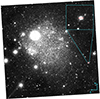 |
Fig. 1. Image of the Sextans A galaxy using du Pont 100 inch. The slit drawn on top of Sextans A GC-1 indicates the location of the UVES slit. |
Literature and derived basic parameters of Sextans A and its GC-1.
Sextans A GC-1 was observed with UVES on the ESO Very Large Telescope (Dekker et al. 2000) in 2021 (14-15 April, 18-19 April, and 6-7 June). The observation of the target was performed using the red arm and executed in clear conditions and a seeing of  , thin sky transparency, and airmass ranging between 1.06 and 1.39.
The target’s magnitude is V = 18.04 with five hours of observational time, resulting in a signal to noise (S/N) per Å of 160 at 6000 Å. The data were reduced (flat-fielding, wavelength calibration, and flux calibration) using EsoReflex (esoreflex-2.11.5) for UVES (uves-6.1.8). The final spectrum covers the region of 4167–6205 Å. The resolution-slit product of the red arm on UVES is 38 700 and the slit width used was 1.20 arcsec, yielding a spectral resolving power of 33 000 (Dekker et al. 2000).
During the analysis to assess the age estimate, a method from Cabrera-Ziri & Conroy (2022) was applied. For this method it is favourable for a spectrum to contain Ca H+K lines (see Sect. 3.2); therefore, an IL spectrum obtained with OSIRIS, GTC (La Palma) was a better option (Cepa 2010). The observations were performed on March 5 2016 and the data was obtained for and adopted in Beasley et al. (2019). The slit width of 1 arcsec and 2000B grism were used, and the integrated time was 600 s. The data were reduced using IRAF and Python scripts combined. The covered wavelength of the final spectrum is 3947–5693 Å the resolution (FWHM) is 3.0 ± 0.2 Å and the median S/N is 27 Å−1.
3. Analysis
3.1. Models and stellar parameters
The analysis in this study was performed in a similar manner to Larsen et al. (2022), in order for the results to be consistent and comparable. This section covers only the basic overview of the method, while the detailed analysis of high-resolution IL data for star clusters is described in Larsen et al. (2022).
The analysis was performed with a Python3 package called ISPy3 (Larsen et al. 2020). The method uses full spectral synthesis, which automatically accounts for line blending, and one can access a wide variety of elements: α abundances (Mg, Si, Ca, and Ti), Fe-peak elements (Cr, Mn, Fe, Ni, and Sc), heavy elements (Cu, Zn, Zr, Ba, and Eu), and lighter elements such as Na. At first, the spectrum was split up into a number of segments for a pre-analysis step (approximately 100 or 200 Å each); this allowed us to estimate the broadening per segment, which was then used to calculate the mean and standard deviation of the broadening. Subsequently, only regions with lines from specific elements were fitted, and hence spectral windows were provided for each element where their lines are present. Spectral windows were prepared based on the Hinkle et al. (2000) spectrum of Arcturus and the solar spectrum (Kurucz et al. 1984; 2005 version). The spectral windows are the same as in Larsen et al. (2022) with a few exceptions. For some elements, the spectral windows had to be adjusted due to the wavelength coverage of the current data set. A couple of Fe spectral windows were shortened (4952.0–4962.0 Å and 5610.0–5630.0 Å) and one window was excluded completely (5008.0–5017.0 Å). The Mg b triplet (5523.0–5531.0 Å) was excluded as it falls on the edge of the UVES coverage. However, for some of the used spectral windows, the analysis could not find a solution, typically because the spectral features in these windows were too weak to constrain the corresponding abundance at the S/N of our data. The full list of the successfully used spectral windows is given in Table A.1. The table also lists the S/N per Å for each spectral window. These values were computed from the S/N per pixel for reduced data:
where a is the dimensionless number of pixels in one Å: 1 Å ÷ 0.026 Å ≈ 38.
As a starting point for the analysis, we based the spectral modelling on an isochrone with a metallicity similar to that derived from the previous spectroscopic analysis, [Fe/H] = −2.4. In subsequent iterations, the choice of isochrone was updated for consistency with our spectroscopic analysis. In our analysis, the stellar populations were based on the theoretical isochrones of the Dartmouth Stellar Evolution Program (DSEP; Dotter et al. 2007). These isochrones cover stellar populations up to the tip of the RGB evolutionary stage. Therefore, to account for the horizontal branch (HB) stars, photometry of MW GCs was used to complement the DSEP isochrones. The HBs were taken from Advanced Camera for Surveys photometry in Sarajedini et al. (2007) and merged with the isochrones in order to produce a complete Hertzsprung-Russell Diagram (HRD; see Larsen et al. (2022) for details). While other isochrone libraries exist that have more complete coverage of the HRD (including the HB and AGB), we continued using the combination of DSEP isochrones and empirical HB data for consistency with the previous work by Larsen et al. (2022). All these different stellar evolutionary stages from the entire HRD with a combination of HB and DSEP were organised into a set of 98 bins, each with a number of parameters defining the spectral synthesis. The parameters were stellar mass, effective temperature (Teff), the logarithm of surface gravity (log(g)), the radius of the star, the weight of the bin (i.e. the number of stars in the mass range covered by the bin), the logarithm of microturbulent velocity, and the atmospheric model and spectral synthesis codes used to produce the synthetic spectra. The two different combinations were ATLAS12+SYNTHE for stars with Teff > 4000 K (Kurucz 1970) and MARCS+Turbospectrum for the cool stars (Teff < 4000 K) (Gustafsson et al. 2008; Plez 2012). When co-adding the model spectra for each bin to produce an integrated-light spectrum, weights were assigned to each bin, assuming a stellar mass function of the form dN/dM ∝ Mα. A value for the exponent of α = 1 was assumed in order to account for the preferential loss of low-mass stars due to dynamical evolution (Sollima & Baumgardt 2017; Larsen et al. 2022). A lower mass limit of 0.15 M⊙ was assumed. A microturbulent velocity, vturb, for each bin, is described through a linear function of logarithmic surface gravity, log(g):

while for the HB stars the value of the microturbulent velocity was set to vturb = 1.8 km s−1 (Pilachowski et al. 1996; Larsen et al. 2022). The abundances used in the modelling were then iteratively adjusted until the best fit to the observed spectra was obtained. The best fit was estimated based on the χ2 of the difference between the model spectra and the observed spectra, once the model spectra had been scaled to the observed spectrum by means of spline or polynomial fitting functions (to match the continuum levels). The errors for derived abundance values (listed in Table A.1) were assessed when the χ2 value increased by one, compared to the best-fit value, while varying the abundances.
3.2. Analysis of the Sextans A GC-1
In order to define the HRD, an assumption about age and metallicity is required. As discussed above, we used an isochrone with a metallicity that self-consistently matched that derived from our spectral analysis. However, the age was not well constrained by our analysis of the UVES spectra. To verify the values obtained in Beasley et al. (2019), we used the method from Cabrera-Ziri & Conroy (2022). This approach uses the integrated light spectrum to infer the HB properties, age, metallicity, and individual element abundance. For this method, we used the OSIRIS data due to its wavelength coverage. The OSIRIS spectrum has a blue spectral coverage that includes the Ca II H and K lines, which are important for constraining the morphology of the HB. The derived estimate of the age was at least ∼9 Gyr, which is in agreement with Beasley et al. (2019), and this analysis also confirmed that GC-1 is metal-poor, [Fe/H] ∼ −2.00, and that it probably hosts a prominent hot HB population. That said, we should note that although these independent estimates seem consistent with the literature values, the metallicity of this target is outside the regime in which the models used in Cabrera-Ziri & Conroy (2022) were designed to operate (i.e. ∼−1.5 < [Fe/H] < 0.3, see Conroy et al. 2018). Hence, we should sound a note of caution regarding the accuracy of these results.
After a number of iterations including isochrones with various metallicity values, including −2.40 from Beasley et al. (2019) and −2.00 from the above analysis of Cabrera-Ziri & Conroy (2022), the final HRD used corresponded to an α-enhanced isochrone with an age of 9 Gyr and a metallicity of −2.20. The appointed HB was from the Galactic GC NGC 7099, which has a metallicity of [Fe/H] = −2.24 ± 0.02, similar to that of GC-1 (Larsen et al. 2022).
The radial velocity derived from the UVES spectrum is 340.4 ± 0.6 km s−1. It was obtained with an iterative approach in which the radial velocity was determined in a number of the wavelength intervals, from which the mean and the uncertainty on the mean, using the standard deviation, were computed. The derived radial velocity with this method is higher than the earlier determined value of 305 ± 15 km s−1 in Beasley et al. (2019). Sextans A GC-1 then has a radial velocity offset of about 16 km s−1 with respect to the Sextans A (H I) systemic velocity (324 ± 2 km s−1) (Koribalski et al. 2004). The broadening velocity required to fit the model spectra to the UVES observations is σ = 6.67 ± 0.69 km s−1. Once the UVES instrumental broadening of 3.9 km s−1 is subtracted in quadrature (Dekker et al. 2000), the velocity broadening of GC-1 itself becomes 5.41 ± 0.77 km s−1.
4. Results
We have derived the values of iron (Fe), α- (Mg, Ca, Ti, Si), Fe-peak (Cr, Mn, Sc, Ni), and heavy (Ba, Cu, Zn, Eu) element abundances. We also give the non-local thermodynamic equilibrium (NLTE) corrected values for elements for which these have been determined (Mg, Ca, Ti, Mn, Fe, Ni, and Ba) (Eitner et al. 2019; Larsen et al. 2022). The rest of the elements (Si, Cr, Sc, Cu, Zn, and Eu) are unaltered and only the local thermodynamic equilibrium (LTE) values are given.
Each element had one or more spectral windows fitted; Table A.1 provides the full list of wavelength ranges, the derived values (LTE and NLTE), and their uncertainties from ISPy3. These values were used to calculate the final value of each element. The elements with a single spectral window (e.g. Si, Cu, Zn, and Eu) have values directly from ISPy3 output.
For some of the lines, only upper limits were found in some cases (i.e. lines were too weak). In these cases, while the fit converged towards a best-fit value, no lower bound on the uncertainty range was found (i.e. the data are consistent with the complete absence of the line), and hence only a positive error bar is defined. The values and uncertainties listed in Table 2 are the weighted average of the values derived for the spectral windows of every individual element:
![$$ \begin{aligned} \langle [\mathrm{X/Fe} ] \rangle =\frac{\sum w_i[\mathrm{X/Fe} ]_i}{\sum w_i} .\end{aligned} $$](/articles/aa/full_html/2024/05/aa46859-23/aa46859-23-eq4.gif)
Derived abundances.
There are two different uncertainties listed for the final abundance ratio values in the Table 2. The first one is SX – an estimate of the standard error on the mean abundance, which was derived using the weighted standard deviation (SDX, w):
![$$ \begin{aligned} \mathrm{SD} _{\mathrm{X},w}= \left[ \frac{N}{N-1} \frac{\sum (\mathrm{X/Fe} _i - \langle \mathrm{X/Fe} \rangle )^2 w_i}{\sum w_i} \right]^{1/2} \end{aligned} $$](/articles/aa/full_html/2024/05/aa46859-23/aa46859-23-eq5.gif)
The weights were defined as
where σ0 = 0.05 dex was used to account for non-random uncertainties on the derived individual window abundances. Such non-random uncertainties refer to a typical scatter in the abundances between spectral windows that is seen even when spectra of very high S/N are analysed (Larsen et al. 2022).
Another way of estimating the uncertainties on the mean value is to propagate the individual measurement uncertainties, according to the usual formula:
Both estimates of the uncertainties are listed in Table 2. While SX can vary between the LTE and NLTE values depending on how the individual measurements change, σ⟨X⟩ stays the same and is therefore only listed per abundance ratio. In the following, we generally use the larger of the two uncertainties.
To assess how the uncertainty on the velocity dispersion affects our abundance measurements, we performed a test in which we varied the velocity dispersion within the uncertainty range and then repeated the abundance measurements (see the right column in Table 2). The effect is small for the examined range (±0.7 km s−1) and it can be said that velocity broadening is not a strong contribution to the systematic uncertainty. The age difference was explored in previous literature; for example Larsen et al. (2014), where the authors find that the age (within several Gyr) of the input isochrone has only a small effect on the results (< 0.1 dex for [Fe/H] and < 0.05 for abundance ratios [X/Fe].
We used 36 windows containing lines of Fe I and Fe II (see Table A.1 for the list of spectral windows fitted). Sextans A GC-1 was found to be quite metal-poor, [Fe/H] = −2.14 ± 0.04. The abundance ratios of individual α elements differ strongly. In particular, Mg is depleted with respect to the solar value, [Mg/Fe] = −0.79 ± 0.28, while the values for Ca, Ti, and Si are all consistent with super-solar [α/Fe] ratios ([Ca/Fe] = +0.13 ± 0.07, [Ti/Fe] = +0.27 ± 0.11, and [Si/Fe] = +0.62 ± 0.26). The overall α abundance, [α/Fe] = +0.34 ± 0.15, was calculated using only the abundance ratios of [Ca/Fe], [Ti/Fe], and [Si/Fe], due to the extremely depleted [Mg/Fe] value (see Sect. 5.2 for further discussion). Iron-peak elements derived include Sc, Cr, Mn, and Ni. The Fe-peak elements are consistent with scaled-solar or somewhat elevated abundance ratios: [Sc/Fe] = +0.22 ± 0.22, [Cr/Fe] = +0.31 ± 0.18, [Mn/Fe] = +0.19 ± 0.32, and [Ni/Fe] = +0.02 ± 0.12. The heavy elements derived for this GC are Ba, Cu, Zn, and Eu. Ba was derived using three spectral windows. The derived value for the Ba abundance ratio is sub-solar, [Ba/Fe] = −0.38 ± 0.22. The other three elements had a single spectral window and only an upper limit of the abundance was found. The upper limit of Cu is also sub-solar ([Cu/Fe] < −0.355), and for Zn the upper limit is consistent with a scaled-solar composition ([Zn/Fe] < +0.143), whereas the upper limit of Eu allows a significantly super-solar abundance ratio, [Eu/Fe] < +0.766.
The data allowed us to measure the virial mass and the mass-to-light ratio using the line-of-sight velocity broadening of σ = 5.41 ± 0.77 km s−1 calculated in Sect. 3.2. This was then used to calculate the virial mass,
where the half-light radius is taken from Beasley et al. (2019), 7.6 ± 0.2 pc. The same authors obtained the absolute magnitude, MV, 0 = −7.85, from the integrated magnitude, V = 18.04. This results in an unexpectedly high value for the mass-to-light ratio of Mdyn/LV = 4.35 ± 1.40 M⊙/LV⊙ (see Sect. 5.5 for further discussion on this issue).
5. Discussion
5.1. Iron abundance
The derived iron abundance of Sextans A GC-1 shows it to be metal-poor but still well above the metallicity floor, [Fe/H] = −2.14 ± 0.04. Our [Fe/H] determination from the UVES data falls between the two estimates obtained from the OSIRIS spectrum, by Beasley et al. (2019) and the method of Cabrera-Ziri & Conroy (2022), respectively (although see Sect. 3.2 regarding some caveats of these models in this metallicity regime).
Concerning the metallicity of the host galaxy, from the mean V–I colour of the RGB McConnachie (2012) reports ⟨[Fe/H]⟩ ∼ −1.85, while from the colour magnitude diagram (CMD) Dolphin et al. (2003a) estimated ⟨[M/H]⟩ = −1.45 ± 0.20 (with approximate limits of −1.75 < [M/H] < −1.35). Thus, the metallicity range of the metal-poor old populations in Sextans A is extended further towards the low-metallicity tail by GC-1. This means that the present stellar populations could be as low as [Fe/H] = −2.14 ± 0.04.
According to Mateo (1998), Sextans A, WLM, and NGC 6822 have globally similar SF histories as derived from the CMDs. Namely, all three dIrrs had significant SF more than 5–10 Gyr ago, followed by a pause in SF, and then recent SF events within the past Gyr. In Larsen et al. (2022) the iron abundance measured for WLM GC is [Fe/H] = −1.85 ± 0.03, which is more metal-rich compared to Sextans A GC-1; moreover, the iron abundances of three GCs in NGC 6822 were found to be higher than in WLM GC and Sextans A GC-1. Therefore, Sextans A GC-1 is the most metal-poor of the studied GCs within these three galaxies that share similar SF histories.
5.2. α element abundances
The [α/Fe] abundance ratio is susceptible to the ages of stars. This is due to the rapid dispersion of α elements into the ISM by core-collapse SNII from massive stars, occurring on short timescales. In contrast, Fe and Fe-peak elements are dispersed by SNIa, which requires a white dwarf and takes place on longer timescales than SNII (Gilmore & Wyse 1998; Maoz & Mannucci 2012). This means that old stars will be enhanced in [α/Fe] with low metallicities, while younger stars will be depleted in the [α/Fe] ratio but have higher metallicity. This creates a characteristic ‘knee’ in the [α/Fe]–[Fe/H] plane (Tolstoy et al. 2009). α elements can actually be divided into two groups: those formed during a hydrostatic carbon and neon burning (Mg and O) and those formed in the explosion event of Type II supernovae (Si, Ca, and Ti) (Woosley & Weaver 1995; Kobayashi et al. 2006; Pagel 2009).
The derived abundances of Ca, Ti, Si, and Mg, and the mean α abundance, are shown in Fig. 2. In Sextans A GC-1, both [Ca/Fe] and [Ti/Fe] are moderately enhanced. Within the uncertainties, the abundances of Si, Ca, and Ti are all consistent with being enhanced relative to a scaled-solar composition and resemble those typically observed for GCs in the Local Group. In particular, the highlighted GCs in Fig. 2 are: N147 PA-1 (red circle) for [Ca/Fe] and [Si/Fe]; Fornax 3 (red star) for [Ca/Fe], [Ti/Fe], and [Si/Fe]; and M31 358-219 (red square) is the closest match for [Ti/Fe] abundance ratios in Sextans A GC-1. The most occurent GCs that resemble the majority of the element abundances are N147 PA-1 and Fornax 3, hence these two GCs are highlighted in the mean α abundance plot (bottom plot in Fig. 2).
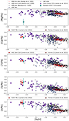 |
Fig. 2. Individual α elements plotted against iron abundance, [Fe/H]. Top: [Mg/Fe] vs. [Fe/H]. Second row: [Ca/Fe] vs. [Fe/H]. Third row: [Ti/Fe] vs. [Fe/H]. Fourth row: [Si/Fe] vs. [Fe/H]. Bottom: [⟨Si, Ca, Ti⟩/Fe] vs. [Fe/H]. Turquoise rhombus refers to this work. Purple circles show the NLTE abundance of the GCs in the Local Group from Larsen et al. (2022); some of these Local Group GCs are highlighted in red symbols and introduced in the legends accordingly, e.g. N147 PA-1 is a red circle, Fornax 3 is a red star, M31 358-219 is a red square, and red crosses and black Xs present MW disc abundances from Reddy et al. (2003, 2006), respectively. Black open circles are the MW disc abundances from Bensby et al. (2005). Blue squares and stars belong to LMC bar and inner disc abundances presented by Van der Swaelmen et al. 2013). |
The derived Mg abundance ratio value for Sextans A GC-1 is extremely depleted, [Mg/Fe] = −0.79 ± 0.29. The NLTE corrections for the [Mg/Fe] abundance ratio were computed at [Mg/Fe] = −0.1 because the grid does not extend to such low [Mg/Fe] ratios. However, it does not influence the conclusions since the NLTE corrections are small (see Table 2) compared to the depletion. There are no GCs that exhibit such a low value of Mg in the Local Group. That is also not in agreement with the value of Mg abundance in the host galaxy that was measured in Kaufer et al. (2004) to be ⟨[α(Mg)/FeII, CrII]⟩ = −0.11 ± 0.02 ± 0.10; however, this value was measured for a young population represented by supergiants (≈10 Myr).
Strongly depleted [Mg/Fe] ratios of extragalactic GCs are frequently found in IL studies, which still remains puzzling (Colucci et al. 2009; Larsen et al. 2012, 2014). An internal spread in the [Mg/Fe] abundance ratios has been observed in some MW GCs, with a fraction of the GC stars having lower [Mg/Fe] ratios than field stars of a corresponding metallicity. One example is M13, for which a sample of stars was examined by Sneden et al. (2004). The study showed clear Na-O and Mg-Al anti-correlations, with a spread in [Mg/Fe] and [Na/Fe] ratios. In particular, [Mg/Fe] varied from −0.2 to +0.4, while [Na/Fe] varied from −0.3 to +0.6. These variations average to [Mg/Fe] = +0.11 and [Na/Fe] = +0.21. The behaviour of these values is similar to the ones derived with IL for WLM GC – [Mg/Fe] = +0.04 ± 0.15 and [Na/Fe] = +0.23 ± 0.15 (Larsen et al. 2014). Another IL study of M13 (Sakari et al. 2013) found [Mg/Fe] = +0.14 ± 0.10 and [Na/Fe] = +0.33 ± 0.16. An even more extreme example is NGC 2419, where [Mg/Fe] ratios of stars extend over from −1 to +1 dex (Mucciarelli et al. 2012, 2018). While these average [Mg/Fe] values (⟨[Mg/Fe]⟩ = +0.05 ± 0.08) are somewhat lower than typical values for field stars, they are not nearly as depleted as the value derived for Sextans A GC-1 from our analysis. Sometimes the [Mg/Fe] ratios are significantly lower than [Ca/Fe] and [Ti/Fe]. The reason for the anomalous [Mg/Fe] ratios in GCs like GC-1 might be linked to a more extreme manifestation of anti-correlations such as those observed in M13, and such internal spreads in the [Mg/Fe] ratio might thus be a common feature within extragalactic GCs. It is however puzzling, then, that no MW GCs exhibit internal Mg abundance variations that are sufficiently large to explain cases like GC-1 (e.g. Pancino et al. 2017). While the environment might be expected to play a role, integrated-light studies of entire galaxies have not uncovered Mg/Fe anomalies as pronounced as those observed in GC-1 (e.g. Kuntschner et al. 2002; Sánchez-Blázquez et al. 2006). However, some evidence for similar abundance patterns has been observed in ultra-faint satellite companions of the Magellanic Clouds such as Car II, with variations in the high-mass end of the IMF suggested as one possible explanation (Ji et al. 2020).
To verify the reliability of the derived value for the [Mg/Fe] abundance ratio, we computed synthetic models for enhanced ([Mg/Fe] = 0.3) and solar ([Mg/Fe] = 0.0) values for Mg abundance ratio. Figure 3 shows the resulting difference between the three models: the best-fit model with depleted Mg in blue, solar Mg in red, enhanced Mg abundance in green, and the observed spectrum in grey. A higher S/N spectrum would lead to a better constraint on [Mg/Fe], but it is already clear from the comparison in Fig. 3 that a favourable model is the depleted Mg model. The reduced χ2 values derived for these three models are 1.138, 1.177, and 1.185 for the depleted, solar, and enhanced models for the Mg line at 4571 Å, while the reduced χ2 values for the Mg line at 4703 Å are similarly 1.306, 1.347, and 1.397 for the depleted, solar, and enhanced models. This test for the used Mg lines at 4571 Å and 4703 Å confirms the Mg deficit in Sextans A GC-1 and the fact that this low abundance of Mg is a favourable solution. Examples of a few other spectral windows and their best fits are given in Figs. 4 and 5.
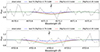 |
Fig. 3. Variation in [Mg/Fe] test. Top: spectral window of the Mg I line at 4571 Å. Bottom: spectral window of the Mg I line at 4703 Å. The best-fit model is in blue, the solar value of [Mg/Fe] is in red, the enhanced [Mg/Fe] abundance is in green, and the observed spectrum is in grey. |
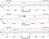 |
Fig. 4. Examples of a few spectral windows used. Top: spectral window at 5328 Å capturing the Fe I lines. Middle: spectral window of Ba II lines at 4934 Å. Bottom: busier spectral region for Ti I lines at 5014–5016 Å with the presence of other elements such as Fe I and Ni I. The best-fit model is in red and the observed spectrum is in grey. |
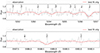 |
Fig. 5. Examples of a couple of spectral windows used to derive Ca. Top: spectral window containing a number of Ca I lines ranging from 5261.0–5266.0 Å with the presence of other elements such as Fe I, Ti I, and Cr I. Bottom: spectral region of Ca I lines at 5588.7 Å and 5590.1 Å. The best-fit model is in red and the observed spectrum is in grey. |
The mean α-abundance, computed by combining all individual α elements except Mg, [⟨Si, Ca, Ti⟩/Fe] = +0.34 ± 0.15, is enhanced at a level that is typical for GCs in the Local Group (Larsen et al. 2022). To summarise, in terms of the α-element abundance, the Sextans A GC mostly resembles GCs in the Local Group, with the one exception of the strongly depleted [Mg/Fe] value.
5.3. Fe-peak element abundances
The Fe-peak elements were produced through thermonuclear reactions in SNIa and massive stars (Kobayashi et al. 2020; Minelli et al. 2021). The derived abundances of Cr, Mn, Sc, and Ni are shown in Fig. 6. The [Cr/Fe] abundance ratio of Sextans A GC-1 is enhanced and it is higher than in the majority of the Local Group GCs. The single cluster that has a higher ratio and is still within the error range is M33 H38, [Cr/Fe] = +0.626 ± 0.161 (red cross in the second plot in Fig. 6).
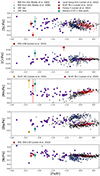 |
Fig. 6. Fe-peak and heavy elements plotted against iron abundance, [Fe/H]. Top: [Sc/Fe] vs. [Fe/H]. Second row: [Cr/Fe] vs. [Fe/H]. Third row: [Mn/Fe] vs. [Fe/H]. Fourth row: [Ba/Fe] vs. [Fe/H]. Bottom: [Ni/Fe] vs. [Fe/H]. Symbols are the same as in Fig. 2. |
The value of Mn abundance derived is solar and resembles some of the GCs within the Local Group: N147 HIII and PA-1. These GCs also show solar and enhanced abundances (shown in yellow and red circles in Fig. 6, respectively). This element has a large uncertainty not only for this cluster but for others as well. This element has only two spectral windows fitted, which results in large uncertainty if the two derived values are not in perfect agreement.
The elevated [Sc/Fe] abundance ratio of this GC fits the Local Group picture. Sc is also often a tracer of α abundance, which is in agreement with Ca, Ti, and Si, which are scaled-solar or enhanced in Sextans A GC-1. In the top plot of Fig. 6 the highlighted GCs are N147 PA-1 (red circle) and Fornax 3 (red star), as these two GCs resembled the majority of the α elements and some Fe-peak elements. It is noticeable here that Sextans A GC-1 and N147 PA-1 are not in perfect agreement for the [Sc/Fe] value; however, this abundance ratio can be quite diverse among Local Group GCs. It ranges between solar 0.0 to enhanced 0.4 dex (Larsen et al. 2022). Another Fe-peak element that resembles the current pattern seen in the Local Group is Ni. The GCs with the closest [Ni/Fe] are Fornax 3 and M31 358-219 (red star and red square in Fig. 6, respectively).
5.4. Heavy element abundances
Heavy elements derived in this study are Ba, Cu, Zn, and Eu. Ba is mainly created by the slow (s-) neutron-capture process (Burris et al. 2000), while Cu and Zn are thought to form via weak s-processing (Pignatari et al. 2010). Eu is mainly created in a rapid neutron-capture (r-) process (Burris et al. 2000). The [Ba/Fe] abundance ratio is depleted to a similar value as in N147 HIII (yellow circle in the fourth plot in Fig. 6). Figure 7 shows the abundances for the Cu, Zn, and Eu abundance ratios. These are the elements for which only the upper limit of the value was found. All of the upper limits appear to be consistent with the current picture of the abundance pattern of the Local Group GCs; for example, M31 358-219 (red square in the first plot in Fig. 7) is particularly close in a value of [Cu/Fe].
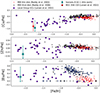 |
Fig. 7. Cu, Zn, and Eu abundance plotted against iron abundance, [Fe/H]. Top: [Cu/Fe] vs. [Fe/H]. Middle: [Zn/Fe] vs. [Fe/H]. Bottom: [Eu/Fe] vs. [Fe/H]. The top of the error bar represents the upper limit derived for the element. The arrow represents all the possible values for this element. Symbols are the same as in Fig. 2. |
5.5. Mass-to-light ratio and dynamical mass
The calculated value for the dynamical mass is Mdyn = (5.18 ± 1.62)×105 M⊙, which is a few times higher than the median mass of GCs in the MW (≈2 × 10⁵ M⊙, e.g. Baumgardt & Hilker 2018). GC-1 is within the ranges found in the Local Group, as significantly more massive GCs with masses well above 106 M⊙ exist in the Local Group (e.g. Strader et al. 2011).
The mass-to-light ratio of Sextans A GC-1 was computed to be high: 4.35 ± 1.40 M⊙/LV⊙. The average value of M/LV in the Local Group is 1.45 M⊙/LV⊙ (McLaughlin 2000), although higher values have been found for GCs in Cen A, NGC 5128, where the ratio varies between 1.1–5 M⊙/LV⊙ (Rejkuba et al. 2008). The latter study also showed an unexpected trend that some blue and metal-poor GCs have rather high mass-to-light ratios of 4–5 M⊙/LV⊙, in contrast to the expectation from simple stellar population models that the M/L ratio should increase with metallicity. Similarly, Strader et al. (2011) found that the optical M/L ratios of M31 GCs decline with increasing metallicity. Given that Sextans A GC-1 is also metal-poor and has a high M/L ratio, it provides another data point that reinforces these trends.
If the dynamical mass is correct – there is no systematic instrumental influence – it could mean a couple of different scenarios that would require different ways to prove or refute them. Kroupa et al. (2013) discussed the possibility of two types of IMF modifications that could enhance the M/L ratio for ultra-compact dwarfs. For a top-heavy IMF, the ratio would be high only if the stellar population were old. This is possible for an old population because the massive stars have become non-luminous remnants. For a bottom-heavy IMF, instead, the M/L ratio is increased because of an excess of faint main-sequence dwarf stars. The two cases are difficult to disentangle by observations, as both populations have low luminosities. There are different tracers to identify the type of IMF. For a bottom-heavy IMF there should be a characteristic absorption feature of CO index in the spectra from low-mass stars (Mieske & Kroupa 2008). If the high M/L ratio is due to a top-heavy IMF then this may be noticeable from low-mass X-ray sources (Kroupa et al. 2013). Another explanation for the high M/L ratio could be the presence of an intermediate-mass black hole (IMBH). An IMBH can be detected through a central rise in the velocity dispersion profile or a shallow central cusp in the surface brightness profile (Hénault-Brunet et al. 2020). Another option might be the presence of more exotic non-stellar mass (i.e. dark matter).
5.6. Age-metallicity relation
Sometimes this relation is used to define the nature of the MW GC – they can be recognised as accreted objects as they appear to follow the accretion branch (i.e. the sequence of decreasing age as a function of increasing metallicity) in the bifurcated age-metallicity relation (AMR) of MW GCs (Leaman et al. 2013a; Carretta & Bragaglia 2022). The steepness of the AMR is dependent on the mass of the host galaxy; in other words, the very old and metal-rich GCs in the MW are those formed in situ. An example of a clear separation between in situ and accreted MW GCs is shown in Forbes & Bridges (2010). This suggests that the detailed age–metallicity distribution of GCs can be used to infer the accretion history of the host galaxy.
Sextans A GC-1 turns out to be more metal-poor for its age when compared to other GCs in Fig. 8. However, one has to be cautious in drawing conclusions from this given the large uncertainty on the age. The closest GC system exhibiting a systematically lower iron abundance at a given age when compared to MW GCs is that of the spiral galaxy NGC 2403, which is also isolated. The two closest to Sextans A GC-1 are JD1 (age = 8.6 ± 2.9 and [Fe/H] = −1.24 ± 0.31) and C4 (age = 12.5 ± 1.6 and [Fe/H] = −2.07 ± 0.18). The system of GCs in NGC 2403 resembles the SMC system for a leaky-box chemical enrichment model (Leaman et al. 2013a). Nevertheless, NGC 2403 GCs lie below other GCs of dwarf galaxies accreted onto the MW. This could be a result of the outflow of enriched material (Fraternali et al. 2002; Dalcanton 2007; Forbes et al. 2022). Another interesting target is the WLM GC, since WLM has spent the majority of its lifetime in isolation (Leaman et al. 2013b). Unfortunately, there is only a single study with the age determined for this target using the V and I photometry bands obtained with Hubble Space Telescope. Based on that study, WLM GC is one of the oldest (14.8 Gyr) with an iron abundance of [Fe/H] = −1.52 ± 0.08 (Hodge et al. 1999). It should be noted that spectroscopic analyses have found a lower metallicity for the WLM GC (Larsen et al. 2022; Colucci & Bernstein 2011). It could be beneficial to revisit this GC to obtain a more accurate age estimate. Hence, while the environment may play a role in setting the AMR for GCs, the WLM GC provides at least one example of a very old, relatively metal-poor GC formed in a low-density environment.
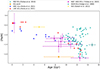 |
Fig. 8. Age vs. [Fe/H] for GCs in the Local Group and NGC 2403. The orange hexagon refers to this work, turquoise circles represent GCs in the MW from Forbes & Bridges (2010), magenta circles represent NGC 2403 GCs from Forbes et al. (2022), the teal circle refers to WLM GCs from Hodge et al. (1999), the yellow circle shows Pal1 from Sakari et al. (2011), and blue and red squares show GCs with reliable parameters (those with confidence code 1) in the SMC and LMC, respectively (Horta et al. 2021). |
The bottom left side of Fig. 8 appears to be underpopulated, which indicates the rarity of young, metal-poor GCs. It would be fascinating to find other isolated GCs to contribute to the same region.
Observational evidence suggests that galaxies in low-density regions tend to form stars with a delay and finish within a longer timescale compared to the galaxies in high-density environments. The SF of field galaxies continues to z ≲ 1 and stays at low-level rates even to the present day, while the ones in clusters finish forming stars at z ≳ 2 (Kuntschner et al. 2002; Thomas et al. 2005). Additionally, early-type galaxies in low-density environments appear ∼1.5 Gyr younger and more metal-rich than in the high-density environments. The favoured scenario is for field galaxies to have a more extended SF history, which results in a less homogeneous stellar population than in the cluster galaxies. Namely, the galaxies in low-density environments are best described by the distribution of the stellar population in which a small portion of young stars is added to an old population (Sánchez-Blázquez et al. 2006). Furthermore, due to the relation found between age and velocity dispersion, authors notice that less-massive galaxies tend to be younger. This seems to be complimentary with the Sextans A and its GC, as it is a dIrr galaxy with a somewhat younger GC of 8.6 ± 2.7 Gyr. This galaxy had continuously formed stars in ancient times, which was followed by a break in SF. Additionally, a small number of stars older than 2.5 Gyr was found, which is again in agreement with Sánchez-Blázquez et al. (2006). This suggests that the SF history of Sextans A is typical of galaxies in low-density environments.
6. Conclusions
Sextans A GC-1 is another cluster that helps populate the low-density environments on the outskirts of the Local Group. It has a curious distribution of α element abundances – extremely metal-poor Mg, solar-scaled or mildly enhanced Ca and Ti, and enhanced Si. In general, this cluster resembles a number of GCs in the Local Group belonging to galaxies such as Fornax and NGC 147. Even though single derived elements resemble the Fornax GCs (Fornax 3 in particular), there is no cluster that would match all of the derived abundances. The depletion of Mg to such a low value cannot be explained up to this moment. Hints of similar (but less extreme) deficiencies of Mg have been observed in the Local Group in GCs such as M13 and NGC 2419 (Sneden et al. 2004; Mucciarelli et al. 2012), but none of these clusters have a [Mg/Fe] ratio as low as that observed in Sextans A GC-1.
Sextans A GC-1 appears to have a high dynamical mass and mass-to-light ratio (Mdyn = (5.18 ± 1.62) × 105 M⊙ and 4.35 ± 1.40 M⊙/LV⊙). This cannot be explained with certainty within this study. A possible solution could include a varying IMF or an IMBH.
This cluster is the first step to start filling up the underpopulated region on the age-metallicity plot. It would be intriguing to find more targets that are metal-poor while being less than 10 Gyr old.
Acknowledgments
We thank the anonymous referee for a careful and critical reading of the manuscript. M.A.B. acknowledges financial support from the grant PID2019-107427GB-C32 from the Spanish Ministry of Science, Innovation and Universities (MCIU) and from the Severo Ochoa Excellence scheme (SEV-2015-0548). This work was backed in part through the IAC project TRACES which is supported through the state budget and the regional budget of the Consejería de Economía, Industria, Comercio y Conocimiento of the Canary Islands Autonomous Community. A.G. thanks Silvia Martocchia for her valuable comments and discussions during this project. This study was supported by the Klaus Tschira Foundation.
References
- Bajkova, A. T., Carraro, G., Korchagin, V. I., Budanova, N. O., & Bobylev, V. V. 2020, ApJ, 895, 69 [NASA ADS] [CrossRef] [Google Scholar]
- Baumgardt, H., & Hilker, M. 2018, MNRAS, 478, 1520 [Google Scholar]
- Beasley, M. A., Leaman, R., Gallart, C., et al. 2019, MNRAS, 487, 1986 [Google Scholar]
- Bell, E. F., Zucker, D. B., Belokurov, V., et al. 2008, ApJ, 680, 295 [Google Scholar]
- Bellazzini, M., Beccari, G., Fraternali, F., et al. 2014, A&A, 566, A44 [NASA ADS] [CrossRef] [EDP Sciences] [Google Scholar]
- Bensby, T., Feltzing, S., Lundström, I., & Ilyin, I. 2005, A&A, 433, 185 [NASA ADS] [CrossRef] [EDP Sciences] [Google Scholar]
- Burris, D. L., Pilachowski, C. A., Armandroff, T. E., et al. 2000, ApJ, 544, 302 [Google Scholar]
- Cabrera-Ziri, I., & Conroy, C. 2022, MNRAS, 511, 341 [NASA ADS] [CrossRef] [Google Scholar]
- Carretta, E., & Bragaglia, A. 2022, A&A, 660, L1 [NASA ADS] [CrossRef] [EDP Sciences] [Google Scholar]
- Cepa, J. 2010, in Highlights of Spanish Astrophysics V, Astrophys. Space Sci. Proc., 14, 15 [NASA ADS] [CrossRef] [Google Scholar]
- Choksi, N., & Gnedin, O. Y. 2019, MNRAS, 486, 331 [NASA ADS] [CrossRef] [Google Scholar]
- Colucci, J. E., & Bernstein, R. A. 2011, in EAS Publications Series, eds. M. Koleva, P. Prugniel, & I. Vauglin, EAS Pub. Ser., 48, 275 [NASA ADS] [CrossRef] [EDP Sciences] [Google Scholar]
- Colucci, J. E., Bernstein, R. A., Cameron, S., McWilliam, A., & Cohen, J. G. 2009, ApJ, 704, 385 [NASA ADS] [CrossRef] [Google Scholar]
- Conroy, C., Villaume, A., van Dokkum, P. G., & Lind, K. 2018, ApJ, 854, 139 [Google Scholar]
- Dalcanton, J. J. 2007, ApJ, 658, 941 [CrossRef] [Google Scholar]
- Dekker, H., D’Odorico, S., Kaufer, A., Delabre, B., & Kotzlowski, H. 2000, in Optical and IR Telescope Instrumentation and Detectors, eds. M. Iye, & A. F. Moorwood, SPIE Conf. Ser., 4008, 534 [Google Scholar]
- Dohm-Palmer, R. C., Skillman, E. D., Saha, A., et al. 1997, AJ, 114, 2527 [Google Scholar]
- Dolphin, A. E., Saha, A., Skillman, E. D., et al. 2003a, AJ, 125, 1261 [Google Scholar]
- Dolphin, A. E., Saha, A., Skillman, E. D., et al. 2003b, AJ, 126, 187 [NASA ADS] [CrossRef] [Google Scholar]
- Dotter, A., Chaboyer, B., Jevremović, D., et al. 2007, AJ, 134, 376 [NASA ADS] [CrossRef] [Google Scholar]
- Eitner, P., Bergemann, M., & Larsen, S. 2019, A&A, 627, A40 [NASA ADS] [CrossRef] [EDP Sciences] [Google Scholar]
- Forbes, D. A., & Bridges, T. 2010, MNRAS, 404, 1203 [NASA ADS] [Google Scholar]
- Forbes, D. A., Bastian, N., Gieles, M., et al. 2018, Proc. R. Soc. London Ser. A, 474, 20170616 [Google Scholar]
- Forbes, D. A., Ferré-Mateu, A., Gannon, J. S., et al. 2022, MNRAS, 512, 802 [NASA ADS] [CrossRef] [Google Scholar]
- Fraternali, F., van Moorsel, G., Sancisi, R., & Oosterloo, T. 2002, AJ, 123, 3124 [CrossRef] [Google Scholar]
- Garcia, M., Herrero, A., Najarro, F., Camacho, I., & Lorenzo, M. 2019, MNRAS, 484, 422 [Google Scholar]
- Georgiev, I. Y., Puzia, T. H., Hilker, M., & Goudfrooij, P. 2009, MNRAS, 392, 879 [NASA ADS] [CrossRef] [Google Scholar]
- Gilmore, G., & Wyse, R. F. G. 1998, AJ, 116, 748 [NASA ADS] [CrossRef] [Google Scholar]
- Gustafsson, B., Edvardsson, B., Eriksson, K., et al. 2008, A&A, 486, 951 [NASA ADS] [CrossRef] [EDP Sciences] [Google Scholar]
- Harris, W. E. 1996, AJ, 112, 1487 [Google Scholar]
- Helmi, A., Babusiaux, C., Koppelman, H. H., et al. 2018, Nature, 563, 85 [Google Scholar]
- Hénault-Brunet, V., Gieles, M., Strader, J., et al. 2020, MNRAS, 491, 113 [CrossRef] [Google Scholar]
- Hinkle, K., Wallace, L., Valenti, J., & Harmer, D. 2000, Visible and Near Infrared Atlas of the Arcturus Spectrum 3727-9300 A (San Francisco: ASP) [Google Scholar]
- Hodge, P. W., Dolphin, A. E., Smith, T. R., & Mateo, M. 1999, ApJ, 521, 577 [NASA ADS] [CrossRef] [Google Scholar]
- Horta, D., Hughes, M. E., Pfeffer, J. L., et al. 2021, MNRAS, 500, 4768 [Google Scholar]
- Huxor, A. P., Mackey, A. D., Ferguson, A. M. N., et al. 2014, MNRAS, 442, 2165 [Google Scholar]
- Ji, A. P., Li, T. S., Simon, J. D., et al. 2020, ApJ, 889, 27 [NASA ADS] [CrossRef] [Google Scholar]
- Kaufer, A., Venn, K. A., Tolstoy, E., Pinte, C., & Kudritzki, R.-P. 2004, AJ, 127, 2723 [NASA ADS] [CrossRef] [Google Scholar]
- Kazantzidis, S., Łokas, E. L., Callegari, S., Mayer, L., & Moustakas, L. A. 2011, ApJ, 726, 98 [NASA ADS] [CrossRef] [Google Scholar]
- Kennicutt, R. C., Jr., & Skillman, E. D. 2001, AJ, 121, 1461 [NASA ADS] [CrossRef] [Google Scholar]
- Kirby, E. N., Cohen, J. G., Guhathakurta, P., et al. 2013, ApJ, 779, 102 [Google Scholar]
- Kobayashi, C., Umeda, H., Nomoto, K., Tominaga, N., & Ohkubo, T. 2006, ApJ, 653, 1145 [NASA ADS] [CrossRef] [Google Scholar]
- Kobayashi, C., Karakas, A. I., & Lugaro, M. 2020, ApJ, 900, 179 [Google Scholar]
- Koribalski, B. S., Staveley-Smith, L., Kilborn, V. A., et al. 2004, AJ, 128, 16 [Google Scholar]
- Kroupa, P., Weidner, C., Pflamm-Altenburg, J., et al. 2013, in Planets, Stars and Stellar Systems. Volume 5: Galactic Structure and Stellar Populations, eds. T. D. Oswalt, & G. Gilmore, 5, 115 [NASA ADS] [Google Scholar]
- Kruijssen, J. M. D. 2019, MNRAS, 486, L20 [NASA ADS] [CrossRef] [Google Scholar]
- Kuntschner, H., Smith, R. J., Colless, M., et al. 2002, MNRAS, 337, 172 [NASA ADS] [CrossRef] [Google Scholar]
- Kurucz, R. L. 1970, SAO Special Report, 309 [Google Scholar]
- Kurucz, R. L., Furenlid, I., Brault, J., & Testerman, L. 1984, Solar Flux Atlas from 296 to 1300 nm (New Mexico: National Solar Observatory) [Google Scholar]
- Larsen, S. S., Brodie, J. P., & Strader, J. 2012, A&A, 546, A53 [NASA ADS] [CrossRef] [EDP Sciences] [Google Scholar]
- Larsen, S. S., Brodie, J. P., Forbes, D. A., & Strader, J. 2014, A&A, 565, A98 [NASA ADS] [CrossRef] [EDP Sciences] [Google Scholar]
- Larsen, S. S., Romanowsky, A. J., Brodie, J. P., & Wasserman, A. 2020, Science, 370, 970 [NASA ADS] [CrossRef] [Google Scholar]
- Larsen, S. S., Romanowsky, A. J., & Brodie, J. P. 2021, A&A, 651, A102 [NASA ADS] [CrossRef] [EDP Sciences] [Google Scholar]
- Larsen, S. S., Eitner, P., Magg, E., et al. 2022, A&A, 660, A88 [NASA ADS] [CrossRef] [EDP Sciences] [Google Scholar]
- Leaman, R., VandenBerg, D. A., & Mendel, J. T. 2013a, MNRAS, 436, 122 [Google Scholar]
- Leaman, R., Venn, K. A., Brooks, A. M., et al. 2013b, ApJ, 767, 131 [NASA ADS] [CrossRef] [Google Scholar]
- Maoz, D., & Mannucci, F. 2012, PASA, 29, 447 [NASA ADS] [CrossRef] [Google Scholar]
- Martin, N. F., Venn, K. A., Aguado, D. S., et al. 2022, Nature, 601, 45 [NASA ADS] [CrossRef] [Google Scholar]
- Mateo, M. L. 1998, ARA&A, 36, 435 [NASA ADS] [CrossRef] [Google Scholar]
- McConnachie, A. W. 2012, AJ, 144, 4 [Google Scholar]
- McLaughlin, D. E. 2000, ApJ, 539, 618 [CrossRef] [Google Scholar]
- Mieske, S., & Kroupa, P. 2008, ApJ, 677, 276 [NASA ADS] [CrossRef] [Google Scholar]
- Minelli, A., Mucciarelli, A., Romano, D., et al. 2021, ApJ, 910, 114 [CrossRef] [Google Scholar]
- Mucciarelli, A., Bellazzini, M., Ibata, R., et al. 2012, MNRAS, 426, 2889 [Google Scholar]
- Mucciarelli, A., Lapenna, E., Ferraro, F. R., & Lanzoni, B. 2018, ApJ, 859, 75 [NASA ADS] [CrossRef] [Google Scholar]
- Pagel, B. E. J. 2009, Nucleosynthesis and Chemical Evolution of Galaxies (Cambridge, UK: Cambridge University Press) [Google Scholar]
- Pancino, E., Romano, D., Tang, B., et al. 2017, A&A, 601, A112 [NASA ADS] [CrossRef] [EDP Sciences] [Google Scholar]
- Pignatari, M., Gallino, R., Heil, M., et al. 2010, ApJ, 710, 1557 [Google Scholar]
- Pilachowski, C. A., Sneden, C., & Kraft, R. P. 1996, AJ, 111, 1689 [Google Scholar]
- Plez, B. 2012, Astrophysics Source Code Library, record [ascl:1205.004] [Google Scholar]
- Reddy, B. E., Tomkin, J., Lambert, D. L., & Allende Prieto, C. 2003, MNRAS, 340, 304 [Google Scholar]
- Reddy, B. E., Lambert, D. L., & Allende Prieto, C. 2006, MNRAS, 367, 1329 [Google Scholar]
- Rejkuba, M., Dubath, P., Minniti, D., & Meylan, G. 2008, in Dynamical Evolution of Dense Stellar Systems, eds. E. Vesperini, M. Giersz, & A. Sills, 246, 418 [NASA ADS] [Google Scholar]
- Sakari, C. M., Venn, K. A., Irwin, M., et al. 2011, ApJ, 740, 106 [NASA ADS] [CrossRef] [Google Scholar]
- Sakari, C. M., Shetrone, M., Venn, K., McWilliam, A., & Dotter, A. 2013, MNRAS, 434, 358 [NASA ADS] [CrossRef] [Google Scholar]
- Sánchez-Blázquez, P., Gorgas, J., Cardiel, N., & González, J. J. 2006, A&A, 457, 809 [NASA ADS] [CrossRef] [EDP Sciences] [Google Scholar]
- Sarajedini, A., Bedin, L. R., Chaboyer, B., et al. 2007, AJ, 133, 1658 [Google Scholar]
- Skillman, E. D., Terlevich, R., Teuben, P. J., & van Woerden, H. 1988, A&A, 198, 33 [NASA ADS] [Google Scholar]
- Sneden, C., Kraft, R. P., Guhathakurta, P., Peterson, R. C., & Fulbright, J. P. 2004, AJ, 127, 2162 [NASA ADS] [CrossRef] [Google Scholar]
- Sollima, A., & Baumgardt, H. 2017, MNRAS, 471, 3668 [NASA ADS] [CrossRef] [Google Scholar]
- Strader, J., Caldwell, N., & Seth, A. C. 2011, AJ, 142, 8 [NASA ADS] [CrossRef] [Google Scholar]
- Thomas, D., Maraston, C., Bender, R., & Mendes de Oliveira, C. 2005, ApJ, 621, 673 [Google Scholar]
- Tolstoy, E., Hill, V., & Tosi, M. 2009, ARA&A, 47, 371 [Google Scholar]
- Van der Swaelmen, M., Hill, V., Primas, F., & Cole, A. A. 2013, A&A, 560, A44 [NASA ADS] [CrossRef] [EDP Sciences] [Google Scholar]
- van Dyk, S. D., Puche, D., & Wong, T. 1998, AJ, 116, 2341 [CrossRef] [Google Scholar]
- Wan, Z., Lewis, G. F., Li, T. S., et al. 2020, Nature, 583, 768 [Google Scholar]
- Woosley, S. E., & Weaver, T. A. 1995, ApJS, 101, 181 [Google Scholar]
Appendix A: Chemical abundances
Chemical abundances of Sextans A GC-1.
All Tables
All Figures
|
Fig. 1. Image of the Sextans A galaxy using du Pont 100 inch. The slit drawn on top of Sextans A GC-1 indicates the location of the UVES slit. |
| In the text | |
|
Fig. 2. Individual α elements plotted against iron abundance, [Fe/H]. Top: [Mg/Fe] vs. [Fe/H]. Second row: [Ca/Fe] vs. [Fe/H]. Third row: [Ti/Fe] vs. [Fe/H]. Fourth row: [Si/Fe] vs. [Fe/H]. Bottom: [⟨Si, Ca, Ti⟩/Fe] vs. [Fe/H]. Turquoise rhombus refers to this work. Purple circles show the NLTE abundance of the GCs in the Local Group from Larsen et al. (2022); some of these Local Group GCs are highlighted in red symbols and introduced in the legends accordingly, e.g. N147 PA-1 is a red circle, Fornax 3 is a red star, M31 358-219 is a red square, and red crosses and black Xs present MW disc abundances from Reddy et al. (2003, 2006), respectively. Black open circles are the MW disc abundances from Bensby et al. (2005). Blue squares and stars belong to LMC bar and inner disc abundances presented by Van der Swaelmen et al. 2013). |
| In the text | |
|
Fig. 3. Variation in [Mg/Fe] test. Top: spectral window of the Mg I line at 4571 Å. Bottom: spectral window of the Mg I line at 4703 Å. The best-fit model is in blue, the solar value of [Mg/Fe] is in red, the enhanced [Mg/Fe] abundance is in green, and the observed spectrum is in grey. |
| In the text | |
|
Fig. 4. Examples of a few spectral windows used. Top: spectral window at 5328 Å capturing the Fe I lines. Middle: spectral window of Ba II lines at 4934 Å. Bottom: busier spectral region for Ti I lines at 5014–5016 Å with the presence of other elements such as Fe I and Ni I. The best-fit model is in red and the observed spectrum is in grey. |
| In the text | |
|
Fig. 5. Examples of a couple of spectral windows used to derive Ca. Top: spectral window containing a number of Ca I lines ranging from 5261.0–5266.0 Å with the presence of other elements such as Fe I, Ti I, and Cr I. Bottom: spectral region of Ca I lines at 5588.7 Å and 5590.1 Å. The best-fit model is in red and the observed spectrum is in grey. |
| In the text | |
|
Fig. 6. Fe-peak and heavy elements plotted against iron abundance, [Fe/H]. Top: [Sc/Fe] vs. [Fe/H]. Second row: [Cr/Fe] vs. [Fe/H]. Third row: [Mn/Fe] vs. [Fe/H]. Fourth row: [Ba/Fe] vs. [Fe/H]. Bottom: [Ni/Fe] vs. [Fe/H]. Symbols are the same as in Fig. 2. |
| In the text | |
|
Fig. 7. Cu, Zn, and Eu abundance plotted against iron abundance, [Fe/H]. Top: [Cu/Fe] vs. [Fe/H]. Middle: [Zn/Fe] vs. [Fe/H]. Bottom: [Eu/Fe] vs. [Fe/H]. The top of the error bar represents the upper limit derived for the element. The arrow represents all the possible values for this element. Symbols are the same as in Fig. 2. |
| In the text | |
|
Fig. 8. Age vs. [Fe/H] for GCs in the Local Group and NGC 2403. The orange hexagon refers to this work, turquoise circles represent GCs in the MW from Forbes & Bridges (2010), magenta circles represent NGC 2403 GCs from Forbes et al. (2022), the teal circle refers to WLM GCs from Hodge et al. (1999), the yellow circle shows Pal1 from Sakari et al. (2011), and blue and red squares show GCs with reliable parameters (those with confidence code 1) in the SMC and LMC, respectively (Horta et al. 2021). |
| In the text | |
Current usage metrics show cumulative count of Article Views (full-text article views including HTML views, PDF and ePub downloads, according to the available data) and Abstracts Views on Vision4Press platform.
Data correspond to usage on the plateform after 2015. The current usage metrics is available 48-96 hours after online publication and is updated daily on week days.
Initial download of the metrics may take a while.