| Issue |
A&A
Volume 659, March 2022
|
|
|---|---|---|
| Article Number | A131 | |
| Number of page(s) | 13 | |
| Section | Extragalactic astronomy | |
| DOI | https://doi.org/10.1051/0004-6361/202140613 | |
| Published online | 17 March 2022 | |
Ionised gas kinematics in MaNGA AGN
Extents of the narrow-line and kinematically disturbed regions⋆
1
Instituto de Astrofisíca de Andalucía, IAA-CSIC, Glorieta de la Astronomia s/n, 18008 Granada, Spain
e-mail: This email address is being protected from spambots. You need JavaScript enabled to view it.
2
Departamento de Física, CCNE, Universidade Federal de Santa Maria, 97105-900 Santa Maria, RS, Brazil
3
Laboratório Interinstitucional de e-Astronomia – LIneA, Rua Gal. José Cristino 77, Rio de Janeiro, RJ 20921-400, Brazil
4
Departamento de Astronomia, Universidade Federal do Rio Grande do Sul, IF, CP 15051, Porto Alegre, 91501-970 RS, Brazil
5
Department of Astronomy and Astrophysics, The Pennsylvania State University, University Park, PA 16802, USA
6
Institute for Gravitation and the Cosmos, The Pennsylvania State University, University Park, PA 16802, USA
7
Apache Point Observatory and New Mexico State University, Sunspot, NM 88349, USA
8
Sternberg Astronomical Institute, Moscow State University, Moscow, Russia
9
Key Laboratory for Research in Galaxies and Cosmology, Shanghai Astronomical Observatory, 80 Nandan Road, Shanghai 200030, PR China
10
University of the Chinese Academy of Sciences, No. 19A Yuquan Road, Beijing 100049, PR China
11
European Southern Observatory, Karl-Schwarzschildstr. 2, 85748 Garching bei München, Germany
12
Observatório Nacional – MCT, Rua General José Cristino 77, Rio de Janeiro, RJ 20921-400, Brazil
13
Universidade do Vale do Paraíba, Av. Shishima Hifumi, 2911, 12244-000 São José dos Campos, SP, Brazil
Received:
19
February
2021
Accepted:
3
January
2022
Abstract
Context. Feedback from active galactic nuclei (AGNs) in general seems to play an important role in the evolution of galaxies, although the impact of AGN winds on their host galaxies is still unknown in the absence of a detailed analysis.
Aims. We aim to analyse the kinematics of a sample of 170 AGN host galaxies as compared to those of a matched control sample of non-active galaxies from the MaNGA survey in order to characterise and estimate the extents of the narrow-line region (NLR) and of the kinematically disturbed region (KDR) by the AGN.
Methods. We defined the observed NLR radius (rNLR, o) as the farthest distance from the nucleus within which both [O III]/Hβ and [N II]/Hα ratios fall in the AGN region of the BPT diagram, and the Hα equivalent width was required to be larger than 3.0 Å. The extent of the KDR (rKDR, o) is defined as the distance from the nucleus within which the AGN host galaxies show a more disturbed gas kinematics than the control galaxies.
Results. The AGN [O III]λ5007 luminosity ranges from 1039 to 1041 erg s−1, and the kinematics derived from the [O III] line profiles reveal that, on average, the most luminous AGNs (L[O III] > 3.8 × 1040 erg s−1) possess higher residual differences between the gaseous and stellar velocities and velocitie dispersions than their control galaxies in all the radial bins. Spatially resolved NLRs and KDRs were found in 55 and 46 AGN host galaxies, with corrected radii 0.2 < rKDR, c < 2.3 kpc and 0.4 < rNLR, c < 10.1 kpc and a relation between the two given by log rKDR, c = (0.53 ± 0.12) log rNLR, c + (1.07 ± 0.22), respectively. On average, the extension of the KDR corresponds to about 30% of that of the NLR. Assuming that the KDR is due to an AGN outflow, we have estimated ionised gas mass outflow rates that range between 10−5 and ∼1 M⊙ yr−1, and kinetic powers that range from 1034 to 1040 erg s−1.
Conclusions. Comparing the power of the AGN ionised outflows with the AGN luminosities, they are always below the 0.05 LAGN model threshold for having an important feedback effect on their respective host galaxies. The mass outflow rates (and power) of our AGN sample correlate with their luminosities, populating the lowest AGN luminosity range of the correlations previously found for more powerful sources.
Key words: galaxies: active / galaxies: kinematics and dynamics / galaxies: general
Tables 1 and 2 are only available at the CDS via anonymous ftp to cdsarc.u-strasbg.fr (130.79.128.5) or via http://cdsarc.u-strasbg.fr/viz-bin/cat/J/A+A/659/A131
© ESO 2022
1. Introduction
Only a small fraction (∼10%) of galaxies are expected to present an active galactic nucleus (AGN, Ho 2008). This phenomenon occurs when the supermassive black hole (SMBH) in the centre of the galaxy captures nearby matter. During this process, this matter is gradually accreted, turning gravitational potential energy into electromagnetic radiation and kinetic energy, by the ejection of particles in the form of winds. The radiation and winds produced in the accretion disk could play an important role in the evolution of the AGN host galaxy – the so-called AGN feedback mechanisms (Cattaneo et al. 2009; Fabian 2012; Harrison 2017). This feedback may influence the evolution of the galaxy, as predicted in cosmological simulations (Croton et al. 2006).
In the unified scheme of AGN (Antonucci 1993; Urry & Padovani 1995), a torus surrounding the accretion disk collimates its radiation, leading to a bi-conical morphology for the narrow-line region (NLR). A similar structure could be expected for the winds launched from the accretion disc, which could also be collimated by the torus. Narrow-band HST images of type 2 quasi-stellar objects (QSOs) reveal elongated ENLRs and bipolar ionisation cones whose extents increase with [O III]λ5007 luminosity (Fischer et al. 2018; Storchi-Bergmann et al. 2018), but in less-luminous Seyfert galaxies the conical morphology is not as common as expected from the unified scheme (Schmitt et al. 2003). He et al. (2018) found bipolar structures with an opening angle of ∼80° in NLRs from MaNGA AGN by analysing emission lines’ ratio behaviours.
The [O III]λ5007 kinematics of the inner kilo-parsec of nearby AGNs reveal that although bi-conical outflows are observed, they appear to be more the exception than the rule. For instance, Mullaney et al. (2013) found that AGN-driven winds due to the interaction of radio jets with the ambient gas usually present a linear structure and not a bi-conical morphology. Fischer et al. (2013) also studied the [O III]λ5007 kinematics in the NLR of 48 Seyfert galaxies and found that in only 12 objects is the ionised gas kinematics consistent with conical outflows, indicating that the gas kinematics of AGNs is more complex than predicted by the unified model. Fischer et al. (2018) investigated the [O III]λ5007 emission distribution and kinematics in a sample of 12 type 2 nearby (z < 0.12) and luminous (log L[O III]/erg s−1 ≳ 42) quasars, using HST observations. They found that the gas is kinematically disturbed by the AGN up to distances of ∼8−15 kpc and determined an average maximum outflow radius of ∼600 pc. Wylezalek et al. (2020) discussed the ionised gas kinematics of a sample of AGNs observed with MaNGA and found that high-velocity gas is more prevalent in AGNs compared to non-AGNs, based on measurements of the line velocity width that encloses 80% of the total flux of the [O III]λ5007 emission line.
Active-galactic-nucleus-driven outflows are known to extend from tens to kpc scales, achieving velocities of hundreds of km s−1 (Crenshaw et al. 2003; Ilha et al. 2019; Wylezalek et al. 2020). However, the impact of these outflows in the AGN host galaxies remains unclear, and recent studies have focused on this question by studying the gas kinematics on large (kpc) scales. Using spatially resolved long-slit spectroscopy, Greene et al. (2011) investigated the kinematics of a sample of 15 nearby (z < 0.5) quasars with [O III]λ5007 luminosity > 1042 erg s−1 and reported that the AGN is the main ionising agent of the interstellar medium over the entire structure of their host galaxies. In powerful AGNs, large-scale outflows are detected, and their extents increase with the AGN luminosity (Greene et al. 2012; Fischer et al. 2018; Storchi-Bergmann et al. 2018). By analysing the [O III]λ5007 and Hβ emitting gas kinematics of a sample of 14 quasars, observed with Gemini IFUs, Liu et al. (2013a) found that all objects possess extended ionised gas nebulae outflows with mean diameter of 28 kpc. Such powerful outflows are able to halt star formation in the host galaxy (e.g. Alatalo et al. 2015). However, Husemann et al. (2016) found that the results from Liu et al. (2013a, 2014) may be affected by not considering beam-smearing effects, which probably indicates that the outflows present smaller extents (Villar-Martín et al. 2016; Karouzos et al. 2016; Tadhunter et al. 2018).
The role of the AGN feedback in low-luminosity AGNs can be addressed with the current surveys of integral field spectroscopy of galaxies, such as the Sloan Digital Sky Survey–IV’s (SDSS-IV; Blanton et al. 2017) Mapping Nearby Galaxies at APO (MaNGA; Bundy et al. 2015) and the Calar Alto Legacy Integral Field Area (CALIFA; Sánchez et al. 2012). We used MaNGA data to investigate the AGN host’s properties, with results presented in the following series of papers. Rembold et al. (2017) discusses nuclear stellar population properties of the first 62 AGNs observed with the MaNGA survey and defined a control sample of inactive galaxies that match the AGN hosts’ properties in terms of stellar mass, redshift, visual morphology, and inclination. It was found that AGNs of increasing luminosity exhibit an increasing contribution from the youngest stellar population relative to control galaxies and a decrease in the oldest components.
The sample defined by Rembold et al. (2017) was used in subsequent studies. Mallmann et al. (2018) presented spatially resolved stellar population properties using the MaNGA data. They showed that the fraction of a young stellar population in high-luminosity AGNs is higher in the inner regions (R ≤ 0.5 Re, where Re is the galaxy effective radius) when compared with the control sample. The low-luminosity AGN and control galaxies display similar fractions of young stars over the whole MaNGA field of view (∼1 Re). do Nascimento et al. (2019) focused on the emission-line flux distributions and gas excitation of this sample and reported that the extent of the region ionised by the AGN is proportional to ![Mathematical equation: $ L_{[{\mathrm{O}\,\textsc{iii}}]}^{0.5} $](/articles/aa/full_html/2022/03/aa40613-21/aa40613-21-eq1.gif) , where L[O III] is the luminosity of the [O III]λ5007 emission line. They also found that the star formation rate is higher in AGNs than in the control galaxies for the early-type host galaxies. The analysis of the nuclear stellar and gas kinematics, as well as the difference of the orientation of the line of nodes derived from the stellar and gas velocity fields (kinematic position angle [PA] offset), is presented in Ilha et al. (2019). By comparing AGN host and inactive galaxies, no difference was found in terms of the kinematic PA offsets between gas and stars. However, AGNs present higher gas velocity dispersion within the inner
, where L[O III] is the luminosity of the [O III]λ5007 emission line. They also found that the star formation rate is higher in AGNs than in the control galaxies for the early-type host galaxies. The analysis of the nuclear stellar and gas kinematics, as well as the difference of the orientation of the line of nodes derived from the stellar and gas velocity fields (kinematic position angle [PA] offset), is presented in Ilha et al. (2019). By comparing AGN host and inactive galaxies, no difference was found in terms of the kinematic PA offsets between gas and stars. However, AGNs present higher gas velocity dispersion within the inner  diameter region, which has been interpreted as being due to AGN-driven outflows.
In the present study, we used an expanded sample relative to that of the above papers, consisting of all AGNs included in the MaNGA Product Launch 8 (MPL-8) (Law et al. 2016), to investigate the large-scale gas kinematics of AGN hosts and compare them to those of a control sample of inactive galaxies, drawn in the same way as in Rembold et al. (2017). Our AGN sample consists of 170 AGNs and two control galaxies for each AGN host. This paper is organised as follows. Section 2 presents a brief description of the MaNGA survey and discusses the sample properties. In Sect. 3, we describe our measurements. In Sect. 4, we present radial profiles of the kinematic properties of the sample galaxies, which are discussed in Sect. 5. The main conclusions of this work are summarised in Sect. 6. The assumed cosmological parameters in this work are H0 = 70 km s−1 Mpc−1, Ωm = 0.3, and ΩV = 0.7.
2. Data
The MaNGA survey focuses on understanding the formation and evolution of galaxies by mapping the kinematics and physical properties of ∼10 000 nearby galaxies, with the redshift (z) ranging from 0.01 to 0.15 and stellar masses greater than 109 M⊙ (Law et al. 2015). The integral field unit (IFU) spectroscopic observations were done with the 2.5-m Sloan telescope of the Apache Point Observatory (APO; Gunn et al. 2006; Smee et al. 2013; Wake et al. 2017; Yan et al. 2016a,b). The spectral resolving power is R ∼ 2000, resulting in an instrumental broadening of σinst = 70 km s−1 (Law et al. 2021), and the average IFU’s angular resolution is  (Yan et al. 2016b; Law et al. 2016). Details about the survey, instrument, and data processing are given in Bundy et al. (2015) and Drory et al. (2015).
The SDSS-IV Data Release (DR) 14 (Abolfathi et al. 2018) includes 2778 MaNGA data cubes. Rembold et al. (2017) presented a sample of all AGN observed by MaNGA in DR14, as obtained from diagnostic diagrams (Baldwin et al. 1981; Cid Fernandes et al. 2010), hereafter called BPT and WHAN diagrams, based on emission-line fluxes and equivalent widths measured using the SDSS-III spectra by Thomas et al. (2013). These diagrams can be used to identify the dominant gas ionisation mechanism in each galaxy and are among the most commonly used diagnostic diagrams to select AGNs using optical observations. To be selected as an AGN host, the galaxy must be located in the Seyfert or LINER region on both BPT and WHAN diagrams simultaneously, including the uncertainties. In order to analyse the effects of AGN on the host galaxies, Rembold et al. (2017) have also selected non-active galaxies to compose a control sample. Two control galaxies were selected for each AGN. This selection was performed by matching the morphology, stellar mass, absolute magnitude, and redshifts of the inactive galaxies to those of the AGN hosts. The initial control sample contains 124 galaxies (12 of them were paired to more than one AGN host). The initial AGN and control samples, as well as their main properties, are listed in Rembold et al. (2017).
After the release of the MaNGA Product Launch 8 (MPL-8), which contains data-cubes for 6779 galaxies, the number of observed AGNs with MaNGA has grown to 173 objects using the same criteria as in Rembold et al. (2017), including the 62 AGNs presented in that work. Following Rembold et al. (2017), we selected two control galaxies for each new AGN, except for three objects: the galaxies identified as MaNGA ID 1-37440, 1-189584, and 31-115. Since these galaxies have low redshifts (z ≲ 0.01), which are close to the lower limit of MaNGA’s redshift range, we were not able to identify control galaxies at similar redshifts. Considering this issue and the fact that the main goal of this paper is to compare the gas kinematics of AGN hosts and their control galaxies, we do not include these objects in the global statistics. The final AGN sample consists of 170 galaxies, with a [O III]λ5007 emission line luminosity ranging from 1039 to 1041 erg s−1, as measured from the SDSS-III spectra. The AGNs and their respective control galaxies are listed in Tables 1 and 2 (available at the CDS), respectively. Figure 1 presents the location of AGN hosts and control galaxies of our sample in the diagnostic diagrams BPT and WHAN. Figure 2 shows the distributions of redshift (z), stellar mass (M⋆), r-band (Mr) absolute magnitude, and [O III]λ5007 luminosity (L[O III]) of our AGN sample, as compared to that of their associated control galaxies. As in the initial sample (Rembold et al. 2017), the AGN and control samples present similar distributions in all parameters except (L[O III]), which is shifted towards larger values for the AGN hosts. Figure 3 presents the SDSS-III multi-colour images of four representative AGN hosts in our extended sample; that is, those not included in Rembold et al. (2017), and their associated controls.
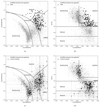 |
Fig. 1. BPT (left) and WHAN (right) diagrams for the AGN hosts (top) and control objects (bottom) in our sample. The separating lines in the plots are from Kauffmann et al. (2003), Kewley et al. (2001), and Cid Fernandes et al. (2010). Grey dots represent all the emission-line galaxies in MPL-8. Large black circles represent AGNs and control objects. |
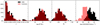 |
Fig. 2. Redshift (z), stellar mass (M⋆), integrated r-band (Mr) absolute magnitude, and [O III]λ5007 distributions for AGN (black) and control samples (red). Both samples are composed mostly of low-luminosity galaxies. |
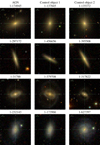 |
Fig. 3. SDSS-III multi-colour images of four representative examples of AGN hosts (left column) and their respective control galaxies (centre and right columns) in our sample. These galaxies were chosen to roughly reproduce the morphological Hubble sequence from ellipticals (top) to late-type spirals (bottom). |
In total, the AGN sample contains 57 early-type (33.5%), 87 late-type (51.2%), and 3 merger galaxies (1.8%), according to the Galaxy Zoo database. There is no classification in Galaxy Zoo for 23 objects (13.5%). Similarly, the control sample is composed of 125 early-type galaxies (36.8%), 182 late-type galaxies (53.5%), 4 merger galaxies (1.2%), and 29 objects (8.5%) whose classifications are uncertain. Regarding the AGN classification, 94 (55.3%) out of the 170 sources present LINER nuclei, while the other 76 (44.7%) galaxies present Seyfert nuclei, as indicated by the BPT diagram (Fig. 1). By visual inspection of the nuclear spectra of all AGN hosts, we conclude that 12 (7.06% of the sample) objects are type 1 AGN (showing broad components in their hydrogen recombination lines). The fraction of type 1 AGN in our sample is smaller than that obtained using SDSS-DR7 spectra, of 10−34% for similar [O III] luminosities (Oh et al. 2015). This difference is likely due to selection effects of the MaNGA sample and by the visual inspection of the observed spectra, which may not be sensitive to faint broad line components. These weak broad components do not affect the determinations of NLR properties, which is the aim of this study.
We have also separated the sample according to the [O III]λ5007 emission line luminosity (L[O III]), which can be used as a proxy for the bolometric luminosity of the AGN (Heckman et al. 2004). The [O III]λ5007 luminosity L[O III] is determined within a circular aperture of  in diameter from the nucleus, based in a single fiber. Following previous works by our group (Rembold et al. 2017; Mallmann et al. 2018; Ilha et al. 2019; do Nascimento et al. 2019), we separated our sample into strong and weak AGNs: strong AGN are defined as those with L[O III] ≥ 3.8 × 1040 erg s−1, measured within a nuclear aperture of 3″ in diameter; weak AGNs are those with L[O III] < 3.8 × 1040 erg s−1. We used the same L[O III], originally proposed by Kauffmann et al. (2003) and that roughly divide their sample in Seyfert (defined by the authors as objects with [O III]5007/Hβ > 3 and [N II]6583/Hα > 0.6) and LINER ([O III]5007/Hβ < 3 and [N II]6583/Hα > 0.6) nuclei. In the complete sample, 62 galaxies can be classified as strong AGNs, which corresponds to 36% of our AGN sample; the new sample includes almost four times the number of strong AGNs when compared to the 17 of Rembold et al. (2017). The number of strong AGNs is slightly smaller than the number of Seyfert nuclei (76), and, for consistency with our previous works, we separated our sample into strong and weak AGNs in this study. The larger number of strong AGNs is relevant, as the main differences in terms of physical properties of the gas and stars of AGN and non-AGN hosts in previous works (Mallmann et al. 2018; Ilha et al. 2019; do Nascimento et al. 2019) were seen in strong AGN. Wylezalek et al. (2020) also observed that the ionised gas kinematics is more extreme in more luminous MaNGA AGNs.
The most important difference between our sample and those of previous studies is that our sample is based on MPL-8, which includes data for 6779 galaxies, while the previous works were based on data release (DR) 14 (Abolfathi et al. 2018), including 2744 galaxies. In addition, this work and that of Wylezalek et al. (2020) used distinct AGN selection criteria. While our selection is based on SDSS-III spectroscopic data from DR 12 (Alam et al. 2015), Wylezalek et al. (2020) used MaNGA data, including off-centred photo-ionisation signatures to classify a galaxy as an AGN (Wylezalek et al. 2018). Finally, an advantage of our work is the selection of a control sample of non-active galaxies with properties matching those of the AGN hosts. This allows us to better investigate the effects of AGN feedback on the host galaxy properties, by making sure that eventual differences are not related to properties such as stellar mass or Hubble type.
3. Measurements
The measurements of the emission-line fluxes and the gas and stellar kinematics from the MaNGA data cubes were performed using the Gas AND Absorption Line Fitting (GANDALF) code (Sarzi et al. 2006), written in interactive data language (IDL). This algorithm maps the gas emission and kinematics while separating the stellar continuum and the gas contributions to the galaxy’s spectra. In order to subtract the continuum spectra and also to measure the stellar kinematics, GANDALF uses the Penalized Pixel-Fitting (PPXF) code (Cappellari & Emsellem 2004; Cappellari 2017). The PPXF code consists of stellar absorption-line fitting, using template spectra as bases. Following Ilha et al. (2019), we used 30 selected evolutionary population synthesis models from Bruzual & Charlot (2003) as template spectra. These models cover ages ranging from 5 Myr to 12 Gyr and three metallicities (0.004 Z⊙, 0.02 Z⊙, 0.05 Z⊙). In addition, we included a multiplicative Legendre polynomial of the order of 3 to account for the different continuum shapes, and the line-of-sight velocity distribution is represented by a Gaussian.
The following emission lines were fitted: Hβ, [O III]λλ4959,5007, [O I]λ6300, [N II]λλ6548,6583, Hα, and [S II]λλ6716,6731. Each emission line is fitted by a single Gaussian component, except for type 1 objects, where a broad component is included to reproduce the nuclear profiles of Hβ and Hα. The centroid velocity and width of the emission lines of the doublets [O III]λλ4959, 5007, [N II]λλ6548, 6583, and [S II]λλ6716, 6731 were kept tied, for each pair separately. During the fit, the following intensity ratios were kept fixed to their theoretical values: [O III]λ5007/[O III]λ4959 = 2.86 and [N II]λ6583/[N II]λ6548 = 2.94 (Osterbrock & Ferland 2006). As discussed in Ilha et al. (2019), the emission-line profiles are well reproduced by single-Gaussian fits; details about the spectral fitting can be found there. In Fig. 4, we present an example of the resulting maps of the properties we derived from our measurements for the AGN host with mangaid 1-48116.
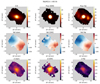 |
Fig. 4. Example of maps we obtained from our measurements for the galaxy MaNGA 1-48116. First row: from left to right, a continuum map in units of 10−17 erg s−1 cm−2 Å−1 obtained by collapsing the whole spectral range, the [O III]5007 Å and Hα flux maps in units of 10−17 erg s−1 cm−2. Second row: from left to right, the stellar, [O III], and Hα velocity fields in km s−1, relatively to the systemic velocity of the galaxy. Bottom row: velocity dispersion maps for the stars, [O III], and Hα, from left to right. In all panels, the north points up and east to the left, and the ΔX and ΔY labels show the distance relative to the peak of the continuum emission. |
To identify and characterise the kinematically disturbed gas by the AGN, we constructed radial profiles of the gas kinematic properties and emission-line ratios. Due to the MaNGA’s spatial resolution and coverage, the radii range that we considered in the present work ranges from 0.5 to 5.0 kpc. We preferred not to correct the radial profiles for projection along the azimuthal direction, because this correction is not clear for many galaxies in our sample. Any bias resulting from this is nevertheless compensated by the fact that the control sample galaxies were selected to present the same aspect ratio of the corresponding AGN. For each galaxy, we calculated the azimuthal median of all values whose spaxels are located within a 0.5 kpc bin, for which the uncertainty in [O III]5007 flux is smaller than 30% and uncertainties in velocity dispersion and centroid velocity are lower than 30 km s−1. Throughout this article, median profiles for properties of the different sub-samples were constructed by computing the median azimuthal values determined within each radial bin. The residual values ([O III] – stars) were calculated at each spaxel and then the median was valued in each radial bin. The differences between the kinematic properties of AGNs and each control galaxy were computed between their azimuthal median profiles.
4. Results
4.1. Excitation
Figure 5 shows median radial profiles of emission-line ratios for the AGN and control samples. We also show bars corresponding to plus and minus the root mean square standard deviation of the quantities, divided by the square root of the number of spaxels. These profiles were used to compare the radial behaviour of the [O III]λ5007/Hβ line ratio of different sub-samples; besides the comparison between AGN and control sample, the panels of Fig. 5 also include the AGN profiles separated into strong and weak sub-samples, as well as in sub-samples of early- and late-type host galaxies.
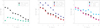 |
Fig. 5. Comparison of the [O III]λ5007/Hβ line ratio spatial profiles. Each point represents the azimuthal median value of the quantities in a bin of 0.5 kpc. The error bars present the standard deviation of the quantities, divided by the square root of the number of spaxels. Left panel: AGN hosts (black) and controls (green); central panel: strong (dark blue) and weak (red) AGNs; right panel: early-type (light blue) and late-type (pink) AGNs. |
Both AGNs’ and control samples’ [O III]λ5007/Hβ ratio profiles decrease with the distance from the nucleus, with a steeper gradient seen for AGNs. Although a few control galaxies do not show gas emission, most of them show some emission, but the median [O III]λ5007/Hβ ratio becomes higher than 1 only in the 1 kpc nuclear bin, while AGNs show a median nuclear [O III]λ5007/Hβ > 3. Strong AGNs display higher [O III]/Hβ ratios for radial distances up to 5 kpc than weak AGNs, indicating that the AGN has a major role in the gas excitation even at large radii. The comparison between early and late-type galaxies reveals that they show similar [O III]/Hβ values at the nucleus, but at distances of 1.5 to 5.0 kpc there are clear differences. While the early-type AGNs have [O III]λ5007/Hβ ≈ 3 over all distances, this ratio decreases for late-type galaxies with increasing distance from the nucleus. Besides probable H II regions dominating the outer regions of the disc of late-type galaxies, another possible explanation for this difference is that, as the amount of gas in early-type galaxies is smaller than in late-type galaxies, the AGN radiation reaches greater distances from the nucleus.
4.2. Kinematics
Figure 6 shows the radial profiles of the kinematic properties of the samples obtained from measurements of the [O III]λ5007 and stellar kinematics. We analysed residual gas velocities and residual velocity dispersion. The residual velocity is defined as the median of the absolute value of [O III]λ5007 velocity minus the velocity of the stars (vres = |v[O III] − vstars|). Likewise, the residual velocity dispersion (σres) is defined as σ[O III] − σstars, where σ is the velocity dispersion. Comparing AGN hosts and controls, the AGNs present higher values of these properties, especially if we only consider the strong AGN. All along the analysed extension, vres for AGN hosts is slightly higher than that for the control galaxies; in strong AGNs, vres is about 10 km s−1 larger than in weak AGNs. Late-type AGNs display similar kinematic properties to that of the control and weak AGN samples. Conversely, early-type AGNs present higher vres than late-type AGNs, increasing with the distance from the nucleus.
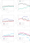 |
Fig. 6. Comparison of median kinematic radial profiles. The symbols and colours are identical to those of Fig. 5. First row: a comparison between AGNs and controls. From left to right: residual between the [O III]λ5007 gas and stellar velocities and residual between the corresponding velocity dispersions. Second row: same as in first row, but comparing strong and weak AGN hosts. Third row: same as first, but comparing early- and late-type AGN hosts. |
The σres profiles shown in the central column panels of Fig. 6 indicate that the velocity dispersion of the control galaxies’ gas is always lower than that of the AGN sample. In the nuclear aperture, the controls display σres ≈ −25.0 km s−1, whilst for AGNs the median value is σres ≈ 2.0 km s−1. Separating the AGN in strong/weak, the highest σres values are dominated by strong AGN all along the analysed extension. While weak AGN do not present positive σres, the strong AGN present it out to 4 kpc from the nucleus. Regarding the early and late-type AGN σres profiles, late-type galaxies show the highest residual velocity dispersion, about 8.0 km s−1 in the nuclear aperture. Early-type galaxies yield negative values of σres in all the analysed bins of radius.
As seen in Fig. 6, the main difference in the kinematics of the AGN and control sample is in the velocity dispersion. A direct comparison of the [O III]λ5007 σ values of AGNs and their controls is shown in Fig. 7. We obtain the median values of the profiles σAGN − σcontrols in three different bins of luminosity: 39.0 ≤ log L[O III] < 40.0 (hereafter low), 40.0 ≤ log L[O III] < 41.0 (hereafter intermediate), and 41.0 ≤ log L[O III] < 42.0 (hereafter high). Each AGN was compared to its respective control galaxies. We define σcontrols = (σcontrol1 + σcontrol2)/2. Low- and intermediate-luminosity AGNs present similar profiles, reaching values of σAGN − σcontrols ∼ 20.0 km s−1 and ∼40.0 km s−1 in the bin corresponding to the inner kpc, respectively. The most luminous AGNs display the highest values of σAGN − σcontrols in all the radial bins. In the inner 1 kpc, this difference reaches ≈65.0 km s−1, indicating a relation between the [O III]λ5007 luminosity and σ.
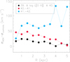 |
Fig. 7. Median radial profile of the σ difference between AGNs and controls. Each AGN was compared to its respective control galaxies. The coloured lines indicate different bins of [O III]λ5007 luminosity, on a logarithmic scale. Over all the analysed extension, the largest differences between an AGN and control velocity dispersions were observed for the most luminous AGN hosts. |
5. Discussion
By comparing the gas kinematics of AGN hosts and control galaxies, we find evidence that the AGNs affect the gas motions up to 4−5 kpc, most clearly seen as differences in the gas velocity dispersion of AGNs and controls, but also observable in the centroid velocities. We attribute these differences to AGN-driven winds interacting with the NLR gas; in this section, we determine the physical extent of these kinematically disturbed regions (KDRs), determine the outflow powers, and discuss their implication for AGN-feedback processes. The KDR is defined here as the region where the gas kinematics is disturbed by the AGN.
5.1. Sizes of the NLR and KDR
5.1.1. Estimates of the NLR and KDR extents
Measurements of the extent of the NLR in AGNs are commonly reported in the literature, mainly based on imaging and integral field spectroscopy (IFS) observations. The extent of the NLR correlates with the AGN luminosity and ranges from a few hundred parsecs in low-luminosity AGNs (e.g. Fraquelli et al. 2003; Schmitt et al. 2003; do Nascimento et al. 2019; Chen et al. 2019) to tens of kpc in the most luminous objects (e.g. Bennert et al. 2002; Greene et al. 2011; Liu et al. 2013a, 2014; Storchi-Bergmann et al. 2018). The KDR extents and how they relate to the size of the NLR is less clear. So far, studies on individual objects and small samples find ionised gas outflows on scales from tens of parsecs to one kiloparsec (Das et al. 2005, 2007; Storchi-Bergmann et al. 2010; Liu et al. 2013b, 2014; Barbosa et al. 2014; Davies et al. 2014; Cresci et al. 2015; Riffel et al. 2013, 2018; Fischer et al. 2017, 2018; Revalski et al. 2018; Diniz et al. 2019; Muñoz Vergara et al. 2019; Soto-Pinto et al. 2019). Here, we measured both the extent of the KDR and the size of the NLR.
We computed the observed extents of the NLR (rNLR, o) and KDR (rKDR, o) of our AGN sample by comparing emission-line ratios and gas kinematics of AGN hosts and control galaxies in bins of 0.5 kpc, although the minimal region considered has a size of two spaxels, which corresponds, on average, to ∼0.876 kpc in our sample. All the bins only take into account the sources that have measurements in the corresponding region; for example, some galaxies do not have the first 0.5 kpc resolved and as consequence are not considered in this bin. We define rNLR, o as the farthest radius from the nucleus within which both [O III]/Hβ and [N II]/Hα emission lines ratios fall in the AGN region of the [O III]/Hβ versus [N II]/Hα BPT diagrams (Baldwin et al. 1981). In addition, the Hα equivalent width was required to be larger than 3.0 Å to exclude regions ionised by post-AGB stars (Stasińska et al. 2008; Cid Fernandes et al. 2011; Singh et al. 2013; Belfiore et al. 2016).
The observed extent of the KDR rKDR, o is defined as the largest radius from the nucleus where the residual σres, AGN = σ[OIII],AGN − σstars, AGN and becomes equal to σres, controls = σ[OIII],controls − σstars, controls. To compare these residuals in both AGN and controls, we fitted their radial distribution by a second-order polynomial and computed the radius where they intercept, which is rKDR, o. The extents rNLR, o and rKDR, o could not be determined for the entire AGN sample, since it was not possible to obtain all the necessary measurements (e.g. when one or both line ratios are AGN-like only for the nuclear aperture, or σres, AGN and σres, controls are already similar at the nucleus).
5.1.2. Are the NLR and KDRs resolved?
The emission-line flux distributions of an unresolved nuclear source can be smeared by the seeing to distances much larger than the FWHM of the point spread function. In order to verify whether the NLR and KDR radii rNLR, o and rKDR, o derived in the previous section are spatially resolved, we followed Kakkad et al. (2020) and computed the [O III]5007 emission-line flux curve of growth (CofG) for each galaxy. We then compared the [O III]5007 flux and PSF CofGs, with the latter obtained from the reconstructed g-band point source profiles included in the MaNGA data cubes. The CofG are not used to estimate the NLR or KDR radii, but just to check if they are spatially resolved by MaNGA. The [O III]5007 emission line is chosen for this purpose because it is the best tracer of the gas ionised by the AGN and of the gas in outflow, with it being one of the strongest optical lines. First, we normalised the [O III] flux by its the value in the nuclear spaxel – defined as that corresponding to the peak of the continuum emission – and then computed the integrated fluxes, increasing the radius in steps of  . The same procedure is adopted to compute the CofG for the PSF.
In Fig. 8, we show examples of the CofGs. We consider that the KDR is spatially resolved if the [O III] flux in the CofG at rKDR, o is higher than that of the PSF considering the 1σ error (i.e. the shaded red region must be above the PSF CofG profile). Similarly, the NLR is considered resolved if at rNLR, o the [O III] flux of the CofG is larger than that of the PSF CofG. The left panel of Fig. 8 shows an example in which both rKDR, o and rNLR, o are spatially resolved, while the right panel shows an example in which the KDR is unresolved and the NLR is resolved. We find that rNLR, o and rKDR, o are spatially resolved in 55 and 46 AGN hosts of our sample, respectively. Our further analysis will be focused on these objects.
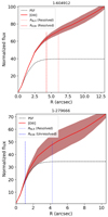 |
Fig. 8. Examples of curves of growth. The black dashed line corresponds to the PSF, and the red line shows the [O III]λ5007 flux and curve of growth. The shaded regions delineate the 1σ flux uncertainties. The vertical dotted and dashed lines show the observed radii of the NLR and KDR, respectively. The mangaid of the galaxies are identified in the title of each panel. |
5.1.3. Correction for the beam smearing effect
Having established that the NLR and KDR of most AGN in our sample are spatially resolved, we now correct their measured extents for beam smearing. In particular, our estimates of the extent of the KDRs are based on kinematic parameters, which are hard to correct using purely photometric techniques like surface brightness deconvolution. In what follows, we simply assume that beam smearing equally affects the derived linear extents obtained from the kinematic and photometric analyses, rKDR, o and rNLR, o, respectively. This assumption allows us to perform a rough correction to the estimated radial extents.
Our methodology for estimating the corrected extents of both the NLR (rNLR, c) and KDR (rKDR, c) is as follows. We start by deconvolving the [O III]5007 brightness profiles of each galaxy, which were derived by calculating the integrated fluxes in concentric rings around the galaxy centre at fixed steps of  in width. The same calculation was performed for the PSF associated with each galaxy (see Sect. 5.1.2). We used these profiles to derive 2D, circularly symmetric flux distributions for [O III] and the PSF with a cubic spline fit, producing ‘pseudo-images’ whose linear scale was lower than the original MaNGA data cubes by a factor of 10. We then performed a 2D Richardson-Lucy deconvolution on the [O III] brightness distributions using the Python package SCIKIT-IMAGE, with the 2D symmetric PSF as input. Finally, in the observed profile we calculated the fraction of the total [O III] flux contained within the raw, uncorrected radial extent of a given structure (KDR or NLR), and impose that the corrected extent comprises the same flux fraction in the deconvolved profile.
Figure 9 shows the comparison between the raw estimates of the extent of the KDR and NLR and those corrected as explained above. The beam smearing, as expected, produces an overestimation of the true extent of both structures. In some cases, particularly for the most extended (≳5″) sources, the corrected sizes are very similar to the raw ones, which was also expected. The mean ratio between the corrected and observed radii are 0.48 ± 0.14 and 0.65 ± 0.22 for rKDR and rNLR, respectively.
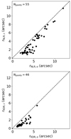 |
Fig. 9. Comparison of the raw estimates of the extents of the NLR (top) and KDR (bottom) with the corrected sizes obtained after deconvolving the [O III] brightness profiles (see text). The dashed lines indicate the locus of the 1:1 relation. |
5.1.4. Comparison between the NLR and KDR extents
Figure 10 displays the rKDR, c against the rNLR, c. The average ⟨rNLR, c⟩ is 3.00 ± 0.33 kpc, and individual values range between 0.4 and 10.1 kpc, which is in good agreement with previous values obtained for MaNGA AGNs based on spatially resolved BPT diagrams (Chen et al. 2019). The KDRs present extents of ⟨rKDR, c⟩ = 0.96 ± 0.09 kpc, varying between 0.2 and 2.3 kpc. Wylezalek et al. (2020) found that the average width of the [OIII]λ5007 line in weak AGNs reaches the same level as non-AGNs at distances of ∼8 kpc from the nucleus, while for strong AGNs similar values are seen at distances of up to 15 kpc, leading to a ‘qualitative’ measurement of the extent of the KDR that are, on average, larger than ours. The p value of the correlation between rKDR, c and rNLR, c of our sources is 10−4, suggesting that they are correlated. We fitted the data by a linear equation and find
 (1)
(1)
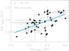 |
Fig. 10. KDR extents versus NLR extents on a logarithmic scale. There is a correlation between these extents, with a Spearman correlation coefficient of CC ∼ 0.53 and a p-value of 10−4. The best-fit linear regression (blue line) results in an intercept of ∼1.07 ± 0.22 and a slope of ∼0.53 ± 0.12. The uncertainties are represented by grey bars corresponding to differences in the value of the properties of 1σ. |
in units of kpc. rKDR, c and rNLR, c present a positive correlation, and, on average, rKDR, c is smaller than rNLR, c, with a mean value of ⟨rKDR, c/rNLR, c⟩ = 0.32 ± 0.27. Using HST observations of 12 nearby type 2 quasars (z < 0.12, Lbol ∼ 1046 erg s−1), Fischer et al. (2018) reported that the extent of the outflows are, on average, only 20% of the extent of the [O III] emission (NLR or ENLR) in a sample of nearby type 2 quasars. Other studies on quasars at larger distances and luminosities (z = 0.5 − 0.6, Lbol ∼ 1047 erg s−1) using integral field spectroscopy and HST images find similar extents for the outflow and ionised gas emission (Liu et al. 2013b, 2014; Wylezalek et al. 2016). As a cautionary note, we point out that the methods used to estimate the size of the KDR and outflows vary widely among all these studies and the comparison between different measurements is not straightforward.
5.2. Mass outflow rates
In order to examine the outflow impact on their host galaxies, we first must estimate the mass outflow rate. Following previous works (e.g. Riffel et al. 2013; Riffel & Storchi-Bergmann 2011; Storchi-Bergmann et al. 2010), we define the mass outflow rate Ṁout as
 (2)
(2)
in which mp is the proton mass, Ne is the electron density, vout is the outflow velocity in the [O III]λ5007 emission line, f is the filling factor, A is the area of the outflow cross-section, and the 1.4 factor is due to the estimated contribution from He to the gas mass. The filling factor can be estimated by
 (3)
(3)
where LHα is the Hα luminosity emitted by a volume V and  erg cm−3 s−1 (Osterbrock & Ferland 2006). Here, we adopt the assumption that all the gas is in outflow, as our data does not allow the separation between gas in the outflow from gas that is not. This assumption may introduce uncertainties that are nevertheless not larger than those introduced by our ignorance of other variables in these calculations, such as the outflow geometry and orientation. Replacing f in Eq. (2) and assuming a spherical geometry for the outflow, we obtain
 (4)
(4)
where r is the radius of the sphere.
As pointed out in the previous section, the radius of the outflow is considered to be smaller than rKDR, c, as previous resolved studies have shown that the mass outflow rates (and powers) (e.g. Storchi-Bergmann et al. 2018; Fischer et al. 2017) usually peak within the inner kpc of the host galaxies and then decrease for larger distances. This ‘peak radius’ is the one to be used in calculations of Ṁout and outflow power, although the effect of the outflows (disturbed kinematics) may extend far beyond this radius. Nevertheless, such radii are not resolved in our MaNGA data. We thus adopted the outflow radius as the smallest value consistent with our observations as the distance corresponding to the radius of the seeing disc of the observation of each source. These values at the galaxies approximately correspond to typical values obtained in resolved studies of ≈1 kpc.
The electron density values were calculated for each galaxy from the [S II]λ6717/[S II]λ6731 ratio and assuming a temperature of 10 000 K. Recent works have argued that the density of the gas in outflow obtained using [S II] is an underestimation for outflows occurring on scales of hundreds of pc, as the [S II] emission originates from a partially ionised region farther out from the nucleus, which has a lower gas density (Baron & Netzer 2019a,b; Davies et al. 2020). However, as the radii of the outflows are of the order of several kpc for our sample, the [S II] emission can be used to obtain the gas density at these distances.
The [S II] doublet is not sensitive to 50 > Ne ≳ 1 × 104 cm−3, where the dependence of the [S II] line ratios with Ne becomes asymptotically flat. Thus, we only estimated the outflow properties in objects with measured densities 50 < Ne < 1 × 104 cm−3. Among the AGN hosts with spatially resolved outflows, we estimate 50 < Ne < 1 × 104 cm−3 for 43 sources. The mass outflow rate and kinetic power of the outflows are estimated only for these objects. In any case, mass outflow rates Ṁout and kinetic power of the outflows Ėkin estimated in this work should be treated as upper limits, the electron density being the major source of uncertainties (e.g. Harrison et al. 2018; Davies et al. 2020).
The differences observed in the gas kinematic profiles of AGN hosts and their controls can be attributed to the nuclear activity. We calculate the outflow velocity as
![Mathematical equation: $$ \begin{aligned} { v}_{\rm out} = |{ v}_{[{\text{O}}{\small {{\text{ II}}}}],\mathrm{AGN}}-{ v}_{\rm stars,AGN}|. \end{aligned} $$](/articles/aa/full_html/2022/03/aa40613-21/aa40613-21-eq12.gif) (5)
(5)
We calculated vout for each galaxy within an aperture corresponding to the MaNGA angular resolution ( FWHM) – adopted as the outflow radius – and then compared each AGN with its respective control galaxy by subtracting their velocities.
The median mass outflow rate of our AGN sample is Ṁout = 7.1 × 10⁻³ M⊙ yr−1. This value is highly uncertain, mainly due to the assumptions regarding the geometry of the outflow and its density. However, by adopting the same assumptions for the whole sample, we can compare the derived mass-outflow rates of all AGN host galaxies. This is done in Fig. 11, which presents Ṁout versus the AGN bolometric luminosity (Lbol). The Lbol was obtained using the following relation from Heckman et al. (2004):
![Mathematical equation: $$ \begin{aligned} L_{\rm bol} \sim 3500 L[{\text{O}}{\small {{\text{ III}}}}], \end{aligned} $$](/articles/aa/full_html/2022/03/aa40613-21/aa40613-21-eq14.gif) (6)
(6)
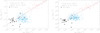 |
Fig. 11. Ṁout (left panel) and Ėkin (right panel) versus the AGN bolometric luminosity. Red circles indicate objects analysed in Fiore et al. (2017), while blue crosses show the objects from Baron & Netzer (2019b). Our sample is represented by black dots, and these characterise AGNs with the lowest luminosity in these relations. We were able to estimate these properties for 20 sources. Black lines show the linear fits considering the three samples. The red dashed lines indicate the linear fit presented in Fiore et al. (2017). |
where L[O III] is the [O III]λ5007 luminosity measured within a circular aperture of  diameter.
For our sample alone, we do not find a strong correlation between Ṁout and L[O III], but the AGNs in our sample span a small luminosity range. For comparison, in Fig. 11 we include the measurements of ionised gas outflows from Fiore et al. (2017) for high-luminosity AGNs (Lbol ≳ 1045 erg s−1) and from Baron & Netzer (2019b) for intermediate-luminosity AGNs (Lbol ≈ 1044 − 1046 erg s−1). Our data fill the low-luminosity end of the relation (Lbol ≈ 1042 − 1045 erg s−1). The galaxies of our sample are equally spread above and below the relation obtained by Fiore et al. (2017) for higher luminosity AGNs (red dashed line). The galaxies from the sample of Baron & Netzer (2019b) fall mostly below the relation due to their adopted smaller distances and higher densities and thus lower mass outflow rates.
In Fig. 11, we have separated the values of Ṁout obtained in the present work, combined with those of Fiore et al. (2017) and Baron & Netzer (2019b), in bins of log Lbol = 0.5 and fitted the average values of Ṁout in these bins as a function of the AGN luminosity Lbol with a linear relation:
 (7)
(7)
which is shown as a black line in the left panel of Fig. 11. However, this result must be taken with caution, as the mass-outflow rates are determined with different methods in the three studies, and the scatter of the relation in the low-luminosity end is large (Shimizu et al. 2019).
5.3. Kinetic power of the outflows
We now obtain the kinetic power of the outflows Ėkin, which is defined as
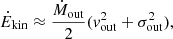 (8)
(8)
in which vout is the outflow velocity defined in Eq. (5). We used the [O III] velocity dispersion as a proxy of σout, which may be a lower limit, as usually the outflows appear as broad wings in the line profiles. We obtain a median value of Ėkin = 5.14 × 1037 erg s−1 for the MaNGA AGN sample. The right panel of Fig. 11 shows Ėkin versus Lbol. As for Ṁout, we included the compilations from Fiore et al. (2017) and Baron & Netzer (2019b). Some of our derived values of Ėkin are on and above the extrapolation of the relation of Fiore et al. (2017), but most are below, similarly to the points from Baron & Netzer (2019b). We obtain the following relation from the fit of the three samples with a linear regression:
 (9)
(9)
which is shown as a black line in the right panel of Fig. 11. We point out that our values of Ėkin may be lower limits, due to our assumed velocity dispersion of the outflow used in the determination of Ėkin.
Numerical simulations (Hopkins & Elvis 2009) indicate that AGN feedback is only important if their kinetic efficiency is Ėkin/Lbol > 5 × 10⁻³, and the AGN feedback becomes more effective when Ėkin is at least ∼5% of the bolometric luminosity (Harrison et al. 2018). In our sample, this occurs only for one source (MaNGA ID 1-258599). Therefore, the majority of outflows detected in our AGN sample are not powerful enough to affect their host galaxies on a large scale. The gas is outflowing from the nucleus and being re-distributed within the galaxies remaining available for further star formation and AGN feeding, comprising the so-called ‘maintenance mode’ AGN feedback. However, the kinetic power of the ionised outflows only corresponds to their mechanical effect in a single gas phase and do not correspond to the initial AGN input energy included in theoretical studies, and thus a comparison between the observed kinetic efficiencies in a specific wind phase and theoretical predictions is not straightforward (e.g. Harrison 2017).
We also measured the escape velocity (Vesc) for each galaxy and find that the outflow velocity is lower than the Vesc in every source, which reinforces the conclusion that the AGN impact is low, the feedback being only in ‘maintenance mode’.
6. Conclusions
We compared the ionised gas kinematics of a sample of 170 active galaxies to those of a control sample of non-active galaxies from the MaNGA survey. Our goal was to look for properties related to the nuclear activity. Using these properties, we estimated the extent of the NLR and of the kinetically disturbed region – KDR (attributed to the interaction of AGN outflows with ambient gas in the host galaxy), showing average kinematic profiles as a function of the radius (in units of effective radius). We also estimated the average values of the mass outflow rate within the inner kpc and the kinetic power of outflows for the AGN sample. Our main conclusions are the following.
-
We find spatially resolved NLRs and KDRs in 55 and 46 AGN host galaxies, respectively, among the 170 AGN of our sample.
-
The main difference in the mean gas excitation of AGN relative to controls was observed in the line ratio [O III]λ5007/Hβ, which was used to obtain the extent of the NLR.
-
The main difference in the kinematic radial profiles of AGNs relative to controls was observed in the residual velocity dispersion σres = σ[O III] − σstars.
-
Over the whole analysed radial extent, the most luminous AGNs (41.0 ≤ log L[O III] ≤ 42.0) present the highest residual velocities vres = |v[O III] − vstars| and residual velocity dispersions σres relative to their respective control galaxies.
-
The NLR extent – adopted as the region where the AGN is the dominant source of ionisation – ranges from 0.4 kpc to 10.1 kpc.
-
The KDR extent ranges from 0.2 to 2.3 kpc, defined as the largest distance from the nucleus where the residual between σ[OIII] and σstars for the AGN and controls become similar. The KDR size is, on average, 32% of the mean NLR extent.
-
There is a correlation between the extent of the KDR and the extent of the NLR; the best fit is rKDR, c = (0.53 ± 0.12)rNLR, c + (1.07 ± 0.22).
-
Assuming that the kinematic disturbance observed along the NLR is due to outflows from the AGN, we estimated the values of the mass outflow rate and power adopting as radius of the outflow the angular resolution of the data.
-
The mass outflow rate ranges between ∼10−5 and ∼1 M⊙ yr−1 and shows a weak correlation with the AGN luminosity.
-
The power of the outflows ranges between ∼1034 and ∼1040 erg s−1 and presents a weak correlation with the AGN luminosity – although this is probably underestimated – with most values below those expected from the extrapolation of the Fiore et al. (2017) relation for more luminous AGNs.
-
The ratio between the kinetic power of the outflow and the AGN bolometric luminosity Ėkin/Lbol ranges between ∼10−7 and 10−4. Only for the AGN with MaNGA ID 1-258599, which is one of the most luminous sources in our sample, is it higher than the 0.5% threshold AGN feedback postulated by models to significantly affect the evolution of the host galaxy.
Although we find that the kinematic disturbance on the NLR by the AGN extends up to several kpc in some galaxies, its effect is not powerful enough to significantly affect their host galaxies. Nevertheless, other gas phases – neutral and molecular – as well as other forms of feedback besides the kinetic one seen in the ionised gas, should also be considered as possible sources of AGN feedback for a fairer comparison with galaxy evolution models.
Acknowledgments
The authors thank the anonymous referee for her/his valu-able suggestions that helped us to significantly improve the present paper. This study was funded in part by the Coordenação de Aperfeiçoamento de Pessoal de Nível Superior – Brasil (CAPES) – Finance Code 001, Conselho Nacional de Desenvolvimento Científico e Tecnológico (CNPq) and Fundação de Amparo à pesquisa do Estado do RS (FAPERGS). ADM acknowledges financial support from the Spanish MCIU grant PID2019-106027GB-C41 and from the State Agency for Research of the Spanish MCIU through the “Center of Excellence Severo Ochoa” award for the Instituto de Astrofísica de Andalucía (SEV-2017-0709). ADM also acknowledges the support of the INPhINIT fellowship form “la Caixa” Foundation (ID 100010434), under the fellowship code LCF/BQ/DI19/11730018. SDSS is managed by the Astrophysical Research Consortium for the Participating Institutions of the SDSS Collaboration including the Brazilian Participation Group, the Carnegie Institution for Science, Carnegie Mellon University, the Chilean Participation Group, the French Participation Group, Harvard-Smithsonian Center for Astrophysics, Instituto de Astrofisica de Canarias, The Johns Hopkins University, Kavli Institute for the Physics and Mathematics of the Universe (IPMU)/University of Tokyo, the Korean Participation Group, Lawrence Berkeley National Laboratory, Leibniz Institut für Astrophysik Potsdam (AIP), Max-Planck-Institut für Astronomie (MPIA Heidelberg), Max-Planck-Institut für Astrophysik (MPA Garching), Max-Planck-Institut für Extraterrestrische Physik (MPE), National Astronomical Observatories of China, New Mexico State University, New York University, University of Notre Dame, Observatório Nacional/MCTI, The Ohio State University, Pennsylvania State University, Shanghai Astronomical Observatory, United Kingdom Participation Group, Universidad Nacional Autónoma de México, University of Arizona, University of Colorado Boulder, University of Oxford, University of Portsmouth, University of Utah, University of Virginia, University of Washington, University of Wisconsin, Vanderbilt University, and Yale University.
References
- Abolfathi, B., Aguado, D. S., Aguilar, G., et al. 2018, ApJS, 235, 42 [NASA ADS] [CrossRef] [Google Scholar]
- Alam, S., Albareti, F. D., Allende Prieto, C., et al. 2015, ApJS, 219, 12 [Google Scholar]
- Alatalo, K., Lacy, M., Lanz, L., et al. 2015, ApJ, 798, 31 [Google Scholar]
- Antonucci, R. 1993, ARA&A, 31, 473 [Google Scholar]
- Baldwin, J. A., Phillips, M. M., & Terlevich, R. 1981, PASP, 93, 5 [Google Scholar]
- Barbosa, F. K. B., Storchi-Bergmann, T., McGregor, P., Vale, T. B., & Riffel, R. A. 2014, MNRAS, 445, 2353 [NASA ADS] [CrossRef] [Google Scholar]
- Baron, D., & Netzer, H. 2019a, MNRAS, 482, 3915 [Google Scholar]
- Baron, D., & Netzer, H. 2019b, MNRAS, 486, 4290 [Google Scholar]
- Belfiore, F., Maiolino, R., Maraston, C., et al. 2016, MNRAS, 461, 3111 [Google Scholar]
- Bennert, N., Falcke, H., Schulz, H., Wilson, A. S., & Wills, B. J. 2002, ApJ, 574, L105 [NASA ADS] [CrossRef] [Google Scholar]
- Blanton, M. R., Bershady, M. A., Abolfathi, B., et al. 2017, AJ, 154, 28 [Google Scholar]
- Bruzual, G., & Charlot, S. 2003, MNRAS, 344, 1000 [NASA ADS] [CrossRef] [Google Scholar]
- Bundy, K., Bershady, M. A., Law, D. R., et al. 2015, ApJ, 798, 7 [Google Scholar]
- Cappellari, M. 2017, MNRAS, 466, 798 [Google Scholar]
- Cappellari, M., & Emsellem, E. 2004, PASP, 116, 138 [Google Scholar]
- Cattaneo, A., Faber, S. M., Binney, J., et al. 2009, Nature, 460, 213 [NASA ADS] [CrossRef] [Google Scholar]
- Chen, J., Shi, Y., Dempsey, R., et al. 2019, MNRAS, 489, 855 [CrossRef] [Google Scholar]
- Cid Fernandes, R., Stasińska, G., Schlickmann, M. S., et al. 2010, MNRAS, 403, 1036 [Google Scholar]
- Cid Fernandes, R., Stasińska, G., Mateus, A., & Vale Asari, N. 2011, MNRAS, 413, 1687 [Google Scholar]
- Crenshaw, D. M., Kraemer, S. B., George, I. M., et al. 2003, ARA&A, 41, 117 [NASA ADS] [CrossRef] [Google Scholar]
- Cresci, G., Marconi, A., Zibetti, S., et al. 2015, A&A, 582, A63 [NASA ADS] [CrossRef] [EDP Sciences] [Google Scholar]
- Croton, D. J., Springel, V., White, S. D. M., et al. 2006, MNRAS, 365, 11 [Google Scholar]
- Das, V., Crenshaw, D. M., Hutchings, J. B., et al. 2005, AJ, 130, 945 [NASA ADS] [CrossRef] [Google Scholar]
- Das, V., Crenshaw, D. M., & Kraemer, S. B. 2007, ApJ, 656, 699 [NASA ADS] [CrossRef] [Google Scholar]
- Davies, R. I., Maciejewski, W., Hicks, E. K. S., et al. 2014, ApJ, 792, 101 [Google Scholar]
- Davies, R., Baron, D., Shimizu, T., et al. 2020, MNRAS, 498, 4150 [Google Scholar]
- Diniz, M. R., Riffel, R. A., Storchi-Bergmann, T., & Riffel, R. 2019, MNRAS, 487, 3958 [NASA ADS] [CrossRef] [Google Scholar]
- do Nascimento, J. C., Storchi-Bergmann, T., Mallmann, N. D., et al. 2019, MNRAS, 486, 5075 [NASA ADS] [CrossRef] [Google Scholar]
- Drory, N., MacDonald, N., Bershady, M. A., et al. 2015, AJ, 149, 77 [CrossRef] [Google Scholar]
- Fabian, A. C. 2012, ARA&A, 50, 455 [Google Scholar]
- Fiore, F., Feruglio, C., Shankar, F., et al. 2017, A&A, 601, A143 [NASA ADS] [CrossRef] [EDP Sciences] [Google Scholar]
- Fischer, T. C., Crenshaw, D. M., Kraemer, S. B., et al. 2013, ApJS, 209, 1 [NASA ADS] [CrossRef] [Google Scholar]
- Fischer, T. C., Machuca, C., Diniz, M. R., et al. 2017, ApJ, 834, 30 [Google Scholar]
- Fischer, T. C., Kraemer, S. B., Schmitt, H. R., et al. 2018, ApJ, 856, 102 [Google Scholar]
- Fraquelli, H. A., Storchi-Bergmann, T., & Levenson, N. A. 2003, MNRAS, 341, 449 [NASA ADS] [CrossRef] [Google Scholar]
- Greene, J. E., Zakamska, N. L., Ho, L. C., et al. 2011, ApJ, 732, 9 [Google Scholar]
- Greene, J. E., Zakamska, N. L., & Smith, P. S. 2012, ApJ, 746, 86 [Google Scholar]
- Gunn, J. E., Siegmund, W. A., Mannery, E. J., et al. 2006, AJ, 131, 2332 [NASA ADS] [CrossRef] [Google Scholar]
- Harrison, C. M. 2017, Nat. Astron., 1, 0165 [NASA ADS] [CrossRef] [Google Scholar]
- Harrison, C. M., Costa, T., Tadhunter, C. N., et al. 2018, Nat. Astron., 2, 198 [Google Scholar]
- He, Z., Sun, A.-L., Zakamska, N. L., et al. 2018, MNRAS, 478, 3614 [Google Scholar]
- Heckman, T. M., Kauffmann, G., Brinchmann, J., et al. 2004, ApJ, 613, 109 [Google Scholar]
- Ho, L. C. 2008, ARA&A, 46, 475 [Google Scholar]
- Hopkins, P. F., & Elvis, M. 2009, MNRAS, 401, 7 [Google Scholar]
- Husemann, B., Scharwächter, J., Bennert, V. N., et al. 2016, A&A, 594, A44 [NASA ADS] [CrossRef] [EDP Sciences] [Google Scholar]
- Ilha, G. S., Riffel, R. A., Schimoia, J. S., et al. 2019, MNRAS, 484, 252 [Google Scholar]
- Kakkad, D., Mainieri, V., Vietri, G., et al. 2020, A&A, 642, A147 [NASA ADS] [CrossRef] [EDP Sciences] [Google Scholar]
- Karouzos, M., Woo, J.-H., & Bae, H.-J. 2016, ApJ, 833, 171 [NASA ADS] [CrossRef] [Google Scholar]
- Kauffmann, G., Heckman, T. M., Tremonti, C., et al. 2003, MNRAS, 346, 1055 [Google Scholar]
- Kewley, L. J., Dopita, M. A., Sutherland, R. S., Heisler, C. A., & Trevena, J. 2001, ApJ, 556, 121 [Google Scholar]
- Law, D. R., Yan, R., Bershady, M. A., et al. 2015, AJ, 150, 19 [CrossRef] [Google Scholar]
- Law, D. R., Cherinka, B., Yan, R., et al. 2016, AJ, 152, 83 [Google Scholar]
- Law, D. R., Westfall, K. B., Bershady, M. A., et al. 2021, AJ, 161, 52 [NASA ADS] [CrossRef] [Google Scholar]
- Liu, G., Zakamska, N. L., Greene, J. E., et al. 2013a, MNRAS, 430, 2327 [NASA ADS] [CrossRef] [Google Scholar]
- Liu, G., Zakamska, N. L., Greene, J. E., Nesvadba, N. P. H., & Liu, X. 2013b, MNRAS, 436, 2576 [NASA ADS] [CrossRef] [Google Scholar]
- Liu, G., Zakamska, N. L., & Greene, J. E. 2014, MNRAS, 442, 1303 [NASA ADS] [CrossRef] [Google Scholar]
- Mallmann, N. D., Riffel, R., Storchi-Bergmann, T., et al. 2018, MNRAS, 478, 5491 [NASA ADS] [CrossRef] [Google Scholar]
- Muñoz Vergara, D., Nagar, N. M., Ramakrishnan, V., et al. 2019, MNRAS, 487, 3679 [CrossRef] [Google Scholar]
- Mullaney, J. R., Alexander, D. M., Fine, S., et al. 2013, MNRAS, 433, 622 [Google Scholar]
- Oh, K., Yi, S. K., Schawinski, K., et al. 2015, ApJS, 219, 1 [Google Scholar]
- Osterbrock, D. E., & Ferland, G. J. 2006, Astrophysics of Gaseous Nebulae and Active Galactic Nuclei (Sausalito, CA: University Science Books) [Google Scholar]
- Rembold, S. B., Shimoia, J. S., Storchi-Bergmann, T., et al. 2017, MNRAS, 472, 4382 [Google Scholar]
- Revalski, M., Crenshaw, D. M., Kraemer, S. B., et al. 2018, ApJ, 856, 46 [NASA ADS] [CrossRef] [Google Scholar]
- Riffel, R. A., & Storchi-Bergmann, T. 2011, MNRAS, 411, 469 [Google Scholar]
- Riffel, R. A., Storchi-Bergmann, T., & Winge, C. 2013, MNRAS, 430, 2249 [Google Scholar]
- Riffel, R. A., Hekatelyne, C., & Freitas, I. C. 2018, PASA, 35, 40 [NASA ADS] [CrossRef] [Google Scholar]
- Sánchez, S. F., Kennicutt, R. C., Gil de Paz, A., et al. 2012, A&A, 538, A8 [Google Scholar]
- Sarzi, M., Falcón-Barroso, J., Davies, R. L., et al. 2006, MNRAS, 366, 1151 [Google Scholar]
- Schmitt, H. R., Donley, J. L., Antonucci, R. R. J., Hutchings, J. B., & Kinney, A. L. 2003, ApJS, 148, 327 [NASA ADS] [CrossRef] [Google Scholar]
- Shimizu, T. T., Davies, R. I., Lutz, D., et al. 2019, MNRAS, 490, 5860 [Google Scholar]
- Singh, R., van de Ven, G., Jahnke, K., et al. 2013, A&A, 558, A43 [NASA ADS] [CrossRef] [EDP Sciences] [Google Scholar]
- Smee, S. A., Gunn, J. E., Uomoto, A., et al. 2013, AJ, 146, 32 [Google Scholar]
- Soto-Pinto, P., Nagar, N. M., Finlez, C., et al. 2019, MNRAS, 489, 4111 [NASA ADS] [CrossRef] [Google Scholar]
- Stasińska, G., Vale Asari, N., Cid Fernandes, R., et al. 2008, MNRAS, 391, L29 [NASA ADS] [Google Scholar]
- Storchi-Bergmann, T., Lopes, R. D. S., McGregor, P. J., et al. 2010, MNRAS, 402, 819 [NASA ADS] [CrossRef] [Google Scholar]
- Storchi-Bergmann, T., Dall’Agnol de Oliveira, B., Longo Micchi, L. F., et al. 2018, ApJ, 868, 14 [Google Scholar]
- Tadhunter, C., Rodríguez Zaurín, J., Rose, M., et al. 2018, MNRAS, 478, 1558 [NASA ADS] [CrossRef] [Google Scholar]
- Thomas, D., Steele, O., Maraston, C., et al. 2013, MNRAS, 431, 1383 [NASA ADS] [CrossRef] [Google Scholar]
- Urry, C. M., & Padovani, P. 1995, PASP, 107, 803 [NASA ADS] [CrossRef] [Google Scholar]
- Villar-Martín, M., Arribas, S., Emonts, B., et al. 2016, MNRAS, 460, 130 [Google Scholar]
- Wake, D. A., Bundy, K., Diamond-Stanic, A. M., et al. 2017, AJ, 154, 86 [Google Scholar]
- Wylezalek, D., Zakamska, N. L., Liu, G., & Obied, G. 2016, MNRAS, 457, 745 [NASA ADS] [CrossRef] [Google Scholar]
- Wylezalek, D., Zakamska, N. L., Greene, J. E., et al. 2018, MNRAS, 474, 1499 [NASA ADS] [CrossRef] [Google Scholar]
- Wylezalek, D., Flores, A. M., Zakamska, N. L., Greene, J. E., & Riffel, R. A. 2020, MNRAS, 492, 4680 [NASA ADS] [CrossRef] [Google Scholar]
- Yan, R., Tremonti, C., Bershady, M. A., et al. 2016a, AJ, 151, 8 [Google Scholar]
- Yan, R., Bundy, K., Law, D. R., et al. 2016b, AJ, 152, 197 [Google Scholar]
All Figures
|
Fig. 1. BPT (left) and WHAN (right) diagrams for the AGN hosts (top) and control objects (bottom) in our sample. The separating lines in the plots are from Kauffmann et al. (2003), Kewley et al. (2001), and Cid Fernandes et al. (2010). Grey dots represent all the emission-line galaxies in MPL-8. Large black circles represent AGNs and control objects. |
| In the text | |
|
Fig. 2. Redshift (z), stellar mass (M⋆), integrated r-band (Mr) absolute magnitude, and [O III]λ5007 distributions for AGN (black) and control samples (red). Both samples are composed mostly of low-luminosity galaxies. |
| In the text | |
|
Fig. 3. SDSS-III multi-colour images of four representative examples of AGN hosts (left column) and their respective control galaxies (centre and right columns) in our sample. These galaxies were chosen to roughly reproduce the morphological Hubble sequence from ellipticals (top) to late-type spirals (bottom). |
| In the text | |
|
Fig. 4. Example of maps we obtained from our measurements for the galaxy MaNGA 1-48116. First row: from left to right, a continuum map in units of 10−17 erg s−1 cm−2 Å−1 obtained by collapsing the whole spectral range, the [O III]5007 Å and Hα flux maps in units of 10−17 erg s−1 cm−2. Second row: from left to right, the stellar, [O III], and Hα velocity fields in km s−1, relatively to the systemic velocity of the galaxy. Bottom row: velocity dispersion maps for the stars, [O III], and Hα, from left to right. In all panels, the north points up and east to the left, and the ΔX and ΔY labels show the distance relative to the peak of the continuum emission. |
| In the text | |
|
Fig. 5. Comparison of the [O III]λ5007/Hβ line ratio spatial profiles. Each point represents the azimuthal median value of the quantities in a bin of 0.5 kpc. The error bars present the standard deviation of the quantities, divided by the square root of the number of spaxels. Left panel: AGN hosts (black) and controls (green); central panel: strong (dark blue) and weak (red) AGNs; right panel: early-type (light blue) and late-type (pink) AGNs. |
| In the text | |
|
Fig. 6. Comparison of median kinematic radial profiles. The symbols and colours are identical to those of Fig. 5. First row: a comparison between AGNs and controls. From left to right: residual between the [O III]λ5007 gas and stellar velocities and residual between the corresponding velocity dispersions. Second row: same as in first row, but comparing strong and weak AGN hosts. Third row: same as first, but comparing early- and late-type AGN hosts. |
| In the text | |
|
Fig. 7. Median radial profile of the σ difference between AGNs and controls. Each AGN was compared to its respective control galaxies. The coloured lines indicate different bins of [O III]λ5007 luminosity, on a logarithmic scale. Over all the analysed extension, the largest differences between an AGN and control velocity dispersions were observed for the most luminous AGN hosts. |
| In the text | |
|
Fig. 8. Examples of curves of growth. The black dashed line corresponds to the PSF, and the red line shows the [O III]λ5007 flux and curve of growth. The shaded regions delineate the 1σ flux uncertainties. The vertical dotted and dashed lines show the observed radii of the NLR and KDR, respectively. The mangaid of the galaxies are identified in the title of each panel. |
| In the text | |
|
Fig. 9. Comparison of the raw estimates of the extents of the NLR (top) and KDR (bottom) with the corrected sizes obtained after deconvolving the [O III] brightness profiles (see text). The dashed lines indicate the locus of the 1:1 relation. |
| In the text | |
|
Fig. 10. KDR extents versus NLR extents on a logarithmic scale. There is a correlation between these extents, with a Spearman correlation coefficient of CC ∼ 0.53 and a p-value of 10−4. The best-fit linear regression (blue line) results in an intercept of ∼1.07 ± 0.22 and a slope of ∼0.53 ± 0.12. The uncertainties are represented by grey bars corresponding to differences in the value of the properties of 1σ. |
| In the text | |
|
Fig. 11. Ṁout (left panel) and Ėkin (right panel) versus the AGN bolometric luminosity. Red circles indicate objects analysed in Fiore et al. (2017), while blue crosses show the objects from Baron & Netzer (2019b). Our sample is represented by black dots, and these characterise AGNs with the lowest luminosity in these relations. We were able to estimate these properties for 20 sources. Black lines show the linear fits considering the three samples. The red dashed lines indicate the linear fit presented in Fiore et al. (2017). |
| In the text | |
Current usage metrics show cumulative count of Article Views (full-text article views including HTML views, PDF and ePub downloads, according to the available data) and Abstracts Views on Vision4Press platform.
Data correspond to usage on the plateform after 2015. The current usage metrics is available 48-96 hours after online publication and is updated daily on week days.
Initial download of the metrics may take a while.