| Issue |
A&A
Volume 656, December 2021
|
|
|---|---|---|
| Article Number | A78 | |
| Number of page(s) | 22 | |
| Section | Galactic structure, stellar clusters and populations | |
| DOI | https://doi.org/10.1051/0004-6361/202141768 | |
| Published online | 08 December 2021 | |
Photo-chemo-dynamical analysis and the origin of the bulge globular cluster Palomar 6⋆
1
Universidade de São Paulo, IAG, Rua do Matão 1226, Cidade Universitária, São Paulo 05508-900, Brazil
e-mail: This email address is being protected from spambots. You need JavaScript enabled to view it.
2
Leibniz-Institut für Astrophysik Potsdam (AIP), An der Sternwarte 16, Potsdam 14482, Germany
3
Instituto de Astronomía, Universidad Nacional Autónoma de México, A. P. 106, 22800
Ensenada, B. C., México
4
Università di Padova, Dipartimento di Astronomia, Vicolo dell’Osservatorio 2, 35122
Padova, Italy
5
INAF-Osservatorio Astronomico di Padova, Vicolo dell’Osservatorio 5, 35122
Padova, Italy
6
Centro di Ateneo di Studi e Attività Spaziali “Giuseppe Colombo” – CISAS, Via Venezia 15, 35131
Padova, Italy
7
Aix Marseille Univ., CNRS, CNES, LAM, 13013
Marseille, France
8
Instituto de Alta Investigación, Universidad de Tarapacá, Casilla 7D, Arica, Chile
9
Institut de Ciències del Cosmos, Universitat de Barcelona (IEEC-UB), Carrer Martí i Franquès 1, 08028
Barcelona, Spain
10
Universidade Federal do Rio Grande do Sul, Departamento de Astronomia, CP 15051, Porto Alegre, 91501-970
Brazil
Received:
11
July
2021
Accepted:
25
August
2021
Abstract
Context. Palomar 6 (Pal6) is a moderately metal-poor globular cluster projected towards the Galactic bulge. A full analysis of the cluster can give hints on the early chemical enrichment of the Galaxy and a plausible origin of the cluster.
Aims. The aim of this study is threefold: a detailed analysis of high-resolution spectroscopic data obtained with the UVES spectrograph at the Very Large Telescope (VLT) at ESO, the derivation of the age and distance of Pal6 from Hubble Space Telescope (HST) photometric data, and an orbital analysis to determine the probable origin of the cluster.
Methods. High-resolution spectra of six red giant stars in the direction of Pal6 were obtained at the 8 m VLT UT2-Kueyen telescope equipped with the UVES spectrograph in FLAMES+UVES configuration. Spectroscopic parameters were derived through excitation and ionisation equilibrium of Fe I and Fe II lines, and the abundances were obtained from spectrum synthesis. From HST photometric data, the age and distance were derived through a statistical isochrone fitting. Finally, a dynamical analysis was carried out for the cluster assuming two different Galactic potentials.
Results. Four stars that are members of Pal 6 were identified in the sample, which gives a mean radial velocity of 174.3 ± 1.6 km s−1 and a mean metallicity of [Fe/H] = −1.10 ± 0.09 for the cluster. We found an enhancement of α-elements (O, Mg, Si, and Ca) of 0.29< [X/Fe] < 0.38 and the iron-peak element Ti of [Ti/Fe] ∼ +0.3. The odd-Z elements (Na and Al) show a mild enhancement of [X/Fe] ∼ +0.25. The abundances of both first- (Y and Zr) and second-peak (Ba and La) heavy elements are relatively high, with +0.4 < [X/Fe] < +0.60 and +0.4 < [X/Fe] < +0.5, respectively. The r-element Eu is also relatively high with [Eu/Fe] ∼ +0.6. One member star presents enhancements in N and Al, with [Al/Fe] > +0.30, this being evidence of a second stellar population, further confirmed with the NaON-Al (anti)correlations. For the first time, we derived the age of Pal 6, which resulted to be 12.4 ± 0.9 Gyr. We also found a low extinction coefficient RV = 2.6 for the Pal 6 projection, which is compatible with the latest results for the highly extincted bulge populations. The derived extinction law results in a distance of 7.67 ± 0.19 kpc from the Sun with an AV = 4.21 ± 0.05. The chemical and photometric analyses combined with the orbital-dynamical analyses point out that Pal 6 belongs to the bulge component probably formed in the main-bulge progenitor.
Conculsions. The present analysis indicates that the globular cluster Pal 6 is located in the bulge volume and that it was probably formed in the bulge in the early stages of the Milky Way formation, sharing the chemical properties with the family of intermediate metallicity very old clusters M 62, NGC 6522, NGC 6558, and HP 1.
Key words: Galaxy: bulge / globular clusters: individual: Palomar 6 / stars: abundances / Hertzsprung-Russell and C-M diagrams / Galaxy: kinematics and dynamics
Observations collected at the European Southern Observatory, Paranal, Chile (ESO), under programmes 0103.D-0828A (PI: M. Valentini); based on observations with the NASA/ESA Hubble Space Telescope, obtained at the Space Telescope Science Institute, which is operated by AURA, Inc. under NASA contract NAS 5-26555 associated with programme GO-14074.
© ESO 2021
1. Introduction
The stellar populations in the Galactic bulge can provide information on its complex formation processes (e.g., Barbuy et al. 2018a; Queiroz et al. 2020a,b; Rojas-Arriagada et al. 2020). The system of globular clusters (GCs) is an important tracer for the study of the formation and evolution of the Galaxy since they retain the chemo-dynamical signatures of the first stages of the Milky Way formation.
It is expected that the oldest stars of the Galaxy have metallicities of [Fe/H] ∼ −3 and are mostly found in the Galactic halo. However, the oldest stars might instead reside mainly in the Galactic bulge (e.g., Tumlinson 2010) with a higher metallicity of [Fe/H] > −1.5 due to the fast early chemical enrichment in the inner Galaxy (Chiappini et al. 2011; Wise et al. 2012; Barbuy et al. 2018a). Analyses of Galactic bulge GCs have demonstrated that the metallicity distribution of their members peaks at [Fe/H] ∼ −1.0 (Bica et al. 2016, and references therein) and that some of these GCs are older than 12.5 Gyr (Miglio et al. 2016; Barbuy et al. 2016, 2018b; Kerber et al. 2019; Ortolani et al. 2019; Oliveira et al. 2020).
Palomar 6 (Pal 6) is a GC projected towards the Galactic bulge (l = 2.10° and b = 1.78°), located in a highly-extincted region with AV > 4.3 (Harris 1996, 2010 edition)1. Despite being a very interesting cluster, information about Pal 6 is conflicting, preventing further analysis, in particular concerning its distance, and consequently in terms of the Galactic component to which Pal 6 should belong. Pal 6 has been considered to belong to the Galactic bulge due to its current position with respect to the Galactic centre (Ortolani et al. 1995; Bica et al. 2016). Lee et al. (2004) suggested that, based on its chemical and kinematic determinations, Pal 6 should belong to an internal component related to a contribution of the halo (inner). Pérez-Villegas et al. (2020) discussed the case of Pal 6 using a distance of d⊙ = 5.8 kpc (Baumgardt et al. 2019), and from their dynamical orbital analysis, they classified the cluster as a thick disc member. This result is opposite to that of Ortolani et al. (1995), which found a distance of d⊙ = 8.9 kpc, placing Pal 6 in the Galactic bulge. Recently, Massari et al. (2019) presented a classification of clusters in terms of their plausible progenitors, indicating whether a cluster originates in a well-defined component of the Galaxy or if it came from one of the merger processes that occurred in the history of the Galaxy, besides other possibilities. They indicated Pal 6 as an unassociated low-energy cluster, again based on the distance estimated by Baumgardt et al. (2019).
The controversy on which Galactic component Pal 6 is part of is also due to an uncertain metallicity. The first metallicity estimations of Pal 6 by Malkan (1981) from a reddening-free index resulted in [Fe/H] ∼ −1.30. Ortolani et al. (1995), from the V versus V − I colour-magnitude diagram (CMD) based on data observed at the ESO NTT-EMMI, found [Fe/H] ∼ −0.40 by the slope of the red giant branch (RGB) and the presence of a red horizontal branch (RHB). Lee & Carney (2002) obtained [Fe/H] = −1.22 ± 0.18 by analysing the slope of the RGB on the near-infrared (NIR) CMD with NICMOS3 JHK bands. Spectroscopic analysis from high-resolution NIR spectra of three RGB stars by the same authors resulted in [Fe/H] = −1.08 ± 0.06. In Lee et al. (2004), a metallicity of [Fe/H] = −1.0 ± 0.1 was confirmed from a high-resolution spectroscopic analysis of five probable member stars observed with the CSHELL spectrograph at the NASA Infrared Telescope Facility.
As part of the present work, we carried out a detailed analysis of Pal 6 from high-resolution spectra obtained with the FLAMES-UVES spectrograph at the ESO Very Large Telescope (VLT). We also provide the first age derivation of Pal 6 and a consistent distance determination based on photometric data from the Hubble Space Telescope (HST). Furthermore, to connect the spectroscopic and photometric analyses, we perform orbital calculations determining the most probable Galactic component to which Pal 6 belongs. Finally, we indicate the probable progenitor for Pal 6.
This work is organised as follows. The spectroscopic and photometric data are described in Sect. 2 along with the membership analysis of the observed stars. Section 3 gives the derivation of photometric stellar parameters as a first guess for the spectroscopic analysis. The final spectroscopic stellar parameters and abundance derivation are presented in Sect. 4. The photometric analysis and derivation of the fundamental parameters age and distance are described in Sect. 5. The orbital analysis and discussion on the origin of Pal 6 are presented in Sect. 6. Finally, our conclusions are drawn in Sect. 7.
2. Data
In this section, we describe the spectroscopic and photometric data, and the proper motion analysis.
2.1. Spectroscopy
The UVES spectra were obtained using the FLAMES-UVES setup centred at 580 nm in the ESO programme 0103.D-0828 (A) (PI: M. Valentini). The ESO programme was coordinated with programme GO11126 (PI: M. Valentini) for Campaign 11 of the K2 satellite (K2 is the re-purposed Kepler mission; Howell et al. 2014): the goal was to obtain asteroseismology for the giants in the proposed GCs. K2 observed four giants in Pal 6, but their UVES spectra were not collected due to clouds and strong winds that affected ESO observations. UVES spectra have a coverage ranging from 480 nm to 680 nm. Six giant stars of Pal 6 were observed, and the log of observations is given in Table 1. The JHKS-combined image of Pal 6 is shown in Fig. 1 and was obtained from the Vista Variables in the Via Lactea (VVV) survey (Saito et al. 2012).
Log of the spectroscopic FLAMES-UVES observations of programme 0103.D-0828 (A), carried out in 2019.
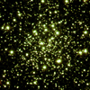 |
Fig. 1. JHKs-combined colour image from the VVV survey for Pal 6. The image has a size of 2 × 2 arcmin2. North is at 45°anticlockwise. |
The data were reduced using the ESO-Reflex software with UVES-Fibre pipeline (Ballester et al. 2000; Modigliani et al. 2004). After reduction, we are left with six spectra for each star. The corresponding spectra of each star were corrected by the radial velocity. To compute the radial velocities and the barycentric corrections, we used the python library PyAstronomy cross-correlating the spectra with the Arcturus spectrum (Hinkle et al. 2000).
The values of heliocentric radial velocity of each spectrum and their mean are presented in Table 2. From these values, we calculate a mean heliocentric radial velocity for Pal 6 of 174.3 ± 1.6 km s−1, excluding the stars ID730 and ID030 for which the radial velocities are very discrepant compared with the other stars. Our mean radial velocity determination is in good agreement with the recent value of 176.3 ± 1.5 km s−1 given by Baumgardt et al. (2019). Finally, each spectrum is normalised and combined through the median flux to obtain the final stellar spectrum.
Radial velocity obtained for each extracted spectra and the average value for each star.
2.2. Photometry
For the photometric analysis, we used the HST data collected during the GO-14074 (PI: Cohen, Cohen et al. 2018) in F110W and F160W (WFC3-IR), and in F606W (ACS-WFC) (first panel of Fig. 2). Data were reduced using the pipeline described in Nardiello et al. (2018). We also followed their recipe (based on the use of the quality-of-fit and photometric error parameters) to select well-measured stars and reject poor photometric measurements. Additionally, we selected the stars within a radius of 300 pixels from the cluster centre that is equivalent to a core radius of ∼0.66 (Harris 1996, 2010 edition). The cleaned CMD is shown in the second panel of Fig. 2, which contains the final selected stars.
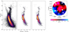 |
Fig. 2. Procedure to obtain the photometry of Pal 6. First panel: HST photometry from Cohen et al. (2018). Second panel: stars selected by the quality method within a radius of ∼0.66 arcmin from the cluster centre. Third panel: differential reddening corrected CMD. Last panel: differential reddening map. |
Another important effect in the photometric data is the differential reddening. Mainly for the clusters with a high reddening value, differential reddening increases the spread on the CMD. This is the case of Pal 6, which has an extinction of AV > 4. We perform a reddening correction with a method similar to that described in Milone et al. (2012). The third panel of Fig. 2 presents the final CMD after the reddening correction is applied, and the map of differential reddening is on the last panel of Fig. 2. The contamination by field stars, combined with the high extincted region, results in low values of differential reddening. However, we obtained clearer main-sequence (MS) turn-off (TO) and sub-giant-branch (SGB) structures for the Pal 6 CMD.
2.3. Membership selection
We performed a membership analysis to find out which stars observed spectroscopically are members of Pal 6. We selected the Gaia Early Data Release 3 (EDR3; Gaia Collaboration 2016) stars within 10′ of the cluster centre (top left panel of Fig. 3). For the proper-motion distribution presented in the bottom left panel of Fig. 3, we applied the Gaussian mixture models (GMMs; Pedregosa et al. 2011) clustering method to separate the cluster members from the field stars. The derived mean proper motion for Pal 6 is 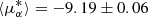 mas yr−1 and ⟨μδ⟩= − 5.30 ± 0.05 mas yr−1, in excellent agreement with the new values computed by Vasiliev & Baumgardt (2021).
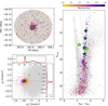 |
Fig. 3. Proper motion analysis to obtain the cluster members. Top left panel: sky distribution of stars within 10 arcmin of the cluster centre. Bottom left panel: vector point diagram with the cluster (coloured dots) and field (grey dots) stars; the green star symbols are the observed stars with FLAMES-UVES, and the insert plots show the density distributions found using GMMs. Right panel: Gaia EDR3 G versus GBP − GRP CMD; the green star symbols are the observed stars. From the bottom left and right panels, we can identify that two observed stars have zero membership probability (yellow star symbols). |
The membership probabilities are computed taking into account both cluster and field distributions, which are derived using GMMs (see Bellini et al. 2009) for the mathematical description of the membership distribution). Once we obtained the membership probability, we cross-matched our sample stars with the Gaia data (Table 3), indicated as green stars in Fig. 3. We found that two stars of our sample have zero membership probability (non-members) and four stars have probabilities above 80%. The non-member stars are the same stars with discrepant radial velocities (ID730 and ID030).
Gaia EDR3 information about the observed stars.
3. Atmospheric stellar paramaters
The photometric effective temperature (Teff) and surface gravity (log g) are derived from the VIJHKS magnitudes given in Table 4. For comparison purposes, we also obtained the effective temperature from the Transiting Exoplanet Survey Satellite (TESS) input catalogue (TIC; Stassun et al. 2018) for five of our six observed stars. We collected the 2MASS J, H, and KS magnitudes from Skrutskie et al. (2006) and the VVV survey (Saito et al. 2012). Finally, according to Alonso et al. (1999), the colour V − I is the best colour index to derive the effective temperature of giant stars. To obtain the V − I colour for our sample, we employed the photometric systems’ relationships G − V = f(GBP − GRP) and G − I = f(GBP − GRP) from Gaia EDR3 (Riello et al. 2021).
Identifications, coordinates, and magnitudes. JHKs are given from both 2MASS and VVV surveys.
3.1. Effective temperatures
Effective temperatures Teff were derived from V − I, V − K, and J − K using the colour-temperature calibrations from Casagrande et al. (2010). The VVV JHK colours were transformed into the 2MASS JHKS system using relations given by Soto et al. (2013). For Pal 6, the distance modulus of (m − M)0 = 13.87, extinction AV = 4.53, and metallicity [Fe/H] = −0.91 were used (Harris 1996, 2010 edition) to perform the reddening correction of the colours. Table 5 lists the derived photometric effective temperatures. The ⟨Teff⟩ is the mean effective temperature considering only values below 5000 K.
Atmospheric parameters derived from photometry using calibrations by Casagrande et al. (2010) for V − I, V − K, J − K, and spectroscopic analysis of Fe lines.
3.2. Surface gravities
To derive the photometric surface gravities log g, we used the ratio log(g*/g⊙) where log g⊙ = 4.44:
 (1)
(1)
We adopted the values of ⟨Teff⟩ from Table 5, M* = 0.85 M⊙, and Mbol⊙ = 4.75. The derived values of the photometric Teff and log g are given in the left columns of Table 5.
4. Abundance analysis
We carried out a detailed abundance analysis by means of ionisation and excitation equilibrium to derive stellar parameters, and line-by-line spectrum synthesis for the derivation of abundance ratios.
4.1. Spectroscopic stellar parameters
To determine the final stellar parameters Teff, log g, metallicity [Fe/H], and microturbulence velocity vt of Pal 6, we measured the equivalent width (EW) for a list of Fe I and Fe II lines using DAOSPEC (Stetson & Pancino 2008). With the purpose of evaluating the impact of blending lines, we remeasured some lines with IRAF, mainly for Fe II. In the line list of Table B.1, we also give the adopted oscillator strengths (log gf) for Fe I lines obtained from VALD3 and NIST databases (Piskunov et al. 1995; Martín et al. 2002) and for Fe II lines from Meléndez & Barbuy (2009).
Using the MARCS grid of atmospheric models (Gustafsson et al. 2008), we extracted the 1D photospheric models for our sample. These CN-mild models consider [α/Fe] = +0.20 for [Fe/H] = −0.50, while [α/Fe] = +0.40 for [Fe/H] ≤ −1.00. For the solar Fe abundance, we adopted ϵ(Fe) = 7.50 (Grevesse & Sauval 1998).
Adopting the mean photometric ⟨Teff⟩ and log g calculated in Sect. 3 as initial guesses, we derived the spectroscopic parameters. Through an iterative method, we obtained the excitation and ionisation equilibrium. The excitation equilibrium means a constant distribution of Fe I versus χexc and is obtained iterating the value of Teff. The similar values of [Fe I/H] and [Fe II/H] indicate that the ionisation equilibrium is reached, obtained by iterating in log g. Finally, the microturbulence velocity vt is obtained by imposing a constant distribution of Fe I abundance versus EW. Figure 4 shows the excitation and ionisation equilibrium for the four member stars.
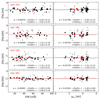 |
Fig. 4. Excitation and ionisation equilibria of Fe I and Fe II lines for the four member stars. The black dots are the values considered to compute the metallicity of Fe I lines after a sigma-clipping of 1 − σ. The crosses are the omitted values. The red squares are the values of Fe II lines. The α values show the slope of the trends of Fe I lines. |
The derived spectroscopic parameters Teff, log g, [Fe I/H], [Fe II/H], [Fe/H], and vt are presented in the right columns of Table 5. Our metallicity determination, based on the four member stars, is [Fe/H] = −1.10 ± 0.09 dex. This metallicty is in excellent agreement with the spectroscopic determinations of Lee & Carney (2002) and Lee et al. (2004), which are [Fe/H] = −1.08 ± 0.06 and −1.0 ± 0.1, respectively.
4.2. Spectrum synthesis
We derived the abundance ratios for the elements C, N, O, Na, Mg, Al, Si, Ca, Ti, Y, Zr, Ba, La, and Eu. For the spectrum synthesis, we employed the PFANT code described in Barbuy et al. (2018c). The code is an update of the Meudon code by M. Spite, and it adopts the local thermodynamic equilibrium (LTE). The basic atomic line list is from VALD3 (Ryabchikova et al. 2015). To obtain the best abundance value, we performed a chi-square minimisation algorithm that fits different values to a region of the spectrum. When needed, a variation on the level of the continuum was taken into account. Figure 5 shows an example of the result obtained with this algorithm for the line of Y I 6435.004 Å of star 243. The blue shaded region represents the best-fit spectrum within 1 − σ, while the grey vertical stripe shows the fit region. The solar abundances A(X) were taken from Grevesse et al. (2015).
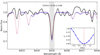 |
Fig. 5. Fit to Y I 6435.004 Å line for star 243. The red dotted lines are the synthetic spectra, the blue strip represents the 1σ region, and the observed spectrum is the black solid line. The values of χ2 are in the insert plot. |
The CNO abundances are listed in Table 6, as detailed below. For the odd-Z, α, and heavy elements, we used the line list from Barbuy et al. (2016). In Table B.2, we give the line-by-line abundance ratios of the odd-Z elements Na and Al; the α-elements Mg, Si, Ca, and Ti; neutron-capture dominant s-elements Y, Zr, La, and Ba; and the r-element Eu. We did not measure Sr lines because they are faint in the observed spectra. The mean values for each star, as well as the cluster mean (considering only the mean of the member stars), are given in Table 7.
Carbon, nitrogen, and oxygen abundances [X/Fe] from C2, CN bandheads, and [OI], respectively.
Abundances in the six UVES sample stars.
4.3. CNO abundances
To measure the CNO abundances we performed an iterative fitting of C, N, and O abundances. For the C abundance, we use the extended C2(1,0) Swan molecular bandhead at 5635.3 Å. We considered the average fit of the region (left panel, Fig. 6) and assumed the abundances as upper limits. For the oxygen (Fig. 6) forbidden line at [OI] 6300.31 Å, a selection among the original spectra where telluric lines did not contaminate the line was needed, since most of the observations were contaminated, showing that these spectra seem to have been observed at too high air masses. A few spectra could be retrieved showing a clean [OI] 6300.31Å line, and the oxygen abundance could be derived. The nitrogen abundance is derived from the CN(5,1) at 6332.2 Å and CN(6,2) at 6478.48 Å of the A2ΠX2Σ system bandheads (Fig. 7). The derived abundances are listed in Table 6.
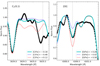 |
Fig. 6. Example for star 243 line fit of the bandhead C2(0,1) (left) and [OI] (right). The solid cyan line is the best-fit abundance ratio, while the dotted lines consider [X/Fe] = [X/Fe]best ± 0.20 (red, plus – blue, minus). |
4.4. Odd-Z elements
We derived the sodium abundances using three NaI lines, one of which is located in the blue arm at 5682.633 Å. The blue-arm spectrum has a S/N lower than the red-arm one. Due to the lower S/N values in all stars, these lines show a higher noise. For this reason, the abundance ratios were essentially derived from the lines located in the red arm, 6154.23 Å and 6160.753 Å.
The aluminium abundances were derived from lines at 6696.185Å and 6698.673 Å. In Fig. 8, we show the Na and Al abundances compared with literature abundances of four other bulge GCs with similar [Fe/H]: M62 (gold; Yong et al. 2014), NGC 6558 (red; Barbuy et al. 2018b), NGC 6522 (green; Barbuy et al. 2021), and HP 1 (purple; Barbuy et al. 2016). For Pal 6, only the member stars are plotted. In general, the abundances are consistent with the other GCs within the uncertainties. The mean value of Pal 6 (pink square) is in good agreement with the other GCs except for M62.
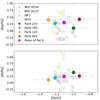 |
Fig. 8. Odd-Z elements, Na (top panel) and Al (bottom panel), abundances as a function of metallicity [Fe/H]. Symbols: Crosses correspond to M 62 (gold; Yong et al. 2014), NGC 6558 (red; Barbuy et al. 2018b), NGC 6552 (green; Barbuy et al. 2021), and HP 1 (purple; Barbuy et al. 2016). The pink square shows the mean value of Pal 6. The filled dots are the mean abundances, together with the error bars. |
4.5. α-elements
The fast early enrichment of the proto-cluster gas by supernovae type II (SNII) can be seen through the abundances of α-elements O, Mg, Ca, and Si, together with Eu produced through the rapid neutron capture process. We obtained a consistent enrichment for all α-elements with a mean value of [α/Fe] = +0.35 and a dispersion of 0.06.
Figure 9 shows the line profile fitting of the Mg I 6318.720 Å, Si I 6142.494 Å, Ca I 5867.562 Å, and Ti I 6336.113 Å for the member star 243. The best fit is represented by the cyan line. We also show the lines considering a variation of 0.20 dex plus (red) and minus (blue) with regard to the best abundance.
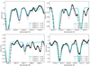 |
Fig. 9. Same as Fig. 6, but for α−elements Mg (top left) Si (top right), Ca (bottom left), and Ti (bottom right). |
We compare the literature abundances of α-elements for the same four GCs NGC 6522, NGC 6558, HP 1, and M 62 in Fig. 10 (Mg in the top panel and Si in the bottom panel) and Fig. 11 (Ca in the top panel and Ti in the bottom panel). These GCs show α enrichment and abundances between ∼0.0 and ∼ + 0.60, which means an average value of ∼0.35. For all elements, the abundances are uniform as functions of [Fe/H].
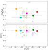 |
Fig. 10. α−elements Mg (top panel) and Si (bottom panel) as functions of metallicity [Fe/H]. The colour code is the same in Fig. 8. |
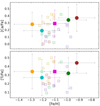 |
Fig. 11. α−elements Ca (top panel) and Ti (bottom panel) as functions of metallicity [Fe/H]. The colour code is the same in Fig. 8. |
4.6. Heavy elements
We derived the abundances of the heavy neutron-capture elements Y, Zr, Ba, La, and Eu. The Eu abundance is essentially the reference for the r-process. We measured the Y I 6435.004 Å and the Y II 6613.73 Å lines. For the final [Y/Fe] values, we assumed that the ionised species of Y contributes 99% to the abundance. Figure 12 shows the line profile fitting of the Y I 6435.004 Å, Ba II 6496.897 Å, La II 6390.477 Å, and Eu II 6437.640 Å for the member star 243. The [Y/Fe] is systematically enhanced for Pal 6 and follows the same pattern observed for the bulge GCs with the same metallicity (top panel of Fig. 13).
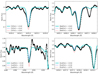 |
Fig. 12. Same as Fig. 6, but for heavy elements Y (top left), Ba (top right), La (bottom left), and Eu (bottom right). |
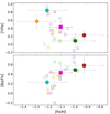 |
Fig. 13. Heavy-elements Y (top panel) and Ba (bottom panel) as a functions of metallicity [Fe/H]. The colour code is the same as in Fig. 8. |
The barium abundance was measured considering only the Ba II 5853.675 Å and 6496.897 Å lines. In the bottom panel of Fig. 13, we show the barium abundances as a function of [Fe/H] compared with the other three bulge GCs. It is possible to observe an opposite pattern compared with [Y/Fe]. The [Ba/Fe] has an enhanced abundance value.
For zirconium, we fit four Zr I lines: 6127.47 Å, 6134.58 Å, 6140.53 Å, and 6143.25 Å. We neglected the strong lines of Zr I located in the blue arm.
The lanthanum abundances are based on five La II lines, which are located at 6172.72 Å, 6262.287 Å, 6296.079 Å, 6320.376 Å, and 6390.477 Å. In Fig. 14, we show the comparison of La abundances with the bulge GCs (top panel). The abundances are in good agreement with the values of the reference GCs. Finally, for the europium abundances, we adopted the lines of Eu II 6437.6 Å and 6645.1 Å. The literature comparison of europium is shown in Fig. 14 (bottom panel).
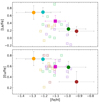 |
Fig. 14. Heavy-elements La (top panel) and Eu (bottom panel) as functions of metallicity [Fe/H]. The colour code is the same as in Fig. 8. |
4.7. Errors
Uncertainties in spectroscopic parameters are given in Table 8 for star 243. For each stellar parameter, we adopted the usual uncertainties as for similar samples (Barbuy et al. 2014, 2016, 2018b): ±100 K in effective temperature, ±0.2 on gravity, and ±0.2 km s−1 on the microturbulence velocity. The sensitivities are computed by employing models with these modified parameters and recomputing lines of different elements considering changes of ΔTeff = +100 K, Δlog g = +0.2, Δvt = 0.2 km s−1. The given error is the difference between the new abundance and the adopted one. Uncertainties due to non-LTE effects are negligible for these stellar parameters as discussed in Ernandes et al. (2018). The same error analysis and estimations can be applied to other stars in our sample. The abundance derivations from strong lines are, in general, avoided, since they are too sensitive to stellar parameters and spectral resolution, as can be seen for the sensitivity of the Ba II lines in Table 8. The La lines are, on the other hand, faint, and they are at least not affected by the same problem. Finally, it is important to note that the main uncertainties in stellar parameters are due to uncertainties in the effective temperature, as can be seen in Table 5. Other significantly important sources of error are the EWs, given the limited S/N of the spectra, which can be estimated by the formula from Cayrel et al. (2004): σEW = 1.5  , where δx is the pixel size.
Sensitivity in abundances due to variation in atmospheric parameters for the star 243, considering uncertainties of ΔTeff = 100 K and Δlog g = 0.2, Δvt = 0.2 km s−1.
4.8. Comparison with previous results
The metallicity derived in this work is in very good agreement with the values derived by Lee & Carney (2002) ([Fe/H] = −1.08 ± 0.06) and Lee et al. (2004) ([Fe/H] = −1.0 ± 0.1) from high-resolution spectroscopy. It is also in good agreement with the Carretta et al. (2009b) metallicity scale, where Pal 6 has [Fe/H] = −1.06 ± 0.09. The metallicity scale of Dias et al. (2016) gives a value of [Fe/H] = −0.85 ± 0.11 for Pal 6. For comparison purposes, we selected the stars of Dias et al. (2016) and calculated their membership probabilities. The stars Pal 6-9 and Pal 6-13 in their sample seem to be members of Pal 6 with metallicities [Fe/H] = −0.76 ± 0.18 and [Fe/H] = −1.14 ± 0.28, respectively. Therefore, we can suppose that the star Pal 6-13 is the most probable member of Pal 6. This shows the power of Gaia, which was not available until very recently, and membership should be verified in all samples preceding the Gaia data.
Recently, Kunder et al. (2021) analysed Pal 6 in the context of the data release 16 (DR16) of the Apache Point Observatory Galactic Evolution Experiment (APOGEE) survey for five observed stars. We inspected the membership probabilities of their sample. With our analysis, all stars are members of the cluster. Their mean radial velocity of 174.5 ± 1.5 is in agreement with our derivation. Their mean metallicity given by the three stars with good ASPCAPFLAG is [Fe/H] = −0.92 ± 0.10, which is compatible within 1 − σ with our result.
We also have abundances for C, N, O, Na, Mg, Si, and Ca elements from APOGEE DR16. The CNO abundances are [C/Fe] = −0.05 ± 0.04, [N/Fe] = +0.31 ± 0.27, and [O/Fe] = +0.22 ± 0.05. These values agreed with our results considering our derived errors; the carbon abundance, which is in excellent agreement with our determination. The abundances of α-elements [Mg/Fe] = +0.34 ± 0.03, [Si/Fe] = +0.22 ± 0.07, and [Ca/Fe] = +0.20 ± 0.03, individually are following the results of Table 7. Additionally, the abundances of α-elements give a value of [α/Fe] = +0.25 ± 0.06, which agrees with our UVES analysis. This value is also in agreement with Coelho et al. (2005): [α/Fe] = +0.28 ± 0.05. Finally, only the two stars with ASPCAPFLAG ≠ 0 have [Na/Fe] values with a mean of [Na/Fe] = +0.35 ± 0.10. However, it is expected that Na should show variations due to the probable presence of first and second generation stars, as discussed below.
4.9. Heavy element analysis
The presence of heavy elements in old stars can be explained through the r-process contribution to these elements, as first suggested by Truran (1981). Otherwise, if an s-process contribution can be identified, the early enhancement of heavy elements can be explained by the ignition of the s-process for the first generation of stars with high rotation, the fast-rotating massive stars (Chiappini et al. 2011; Cescutti et al. 2013, 2015; Frischknecht et al. 2016; Choplin et al. 2018). The rotation transports the 12C from the internal layers to external ones to burn into 14N and 13C. The activation of the s-process occurs when the 14N is converted into 22Ne. Therefore, this mechanism does not predict carbon enhancements.
An alternative explanation is an s-process contribution within a binary system in which the main companion has gone through the asymptotic giant branch (AGB) phase (Beers & Christlieb 2005; Sneden et al. 2008, and references therein). Due to the mass transfer from AGB, the second companion receives s-process yields (see discussion in Barbuy et al. 2021).
The top panel of Fig. 15 highlights the region for the Solar System r-process abundance ratio of [Eu/Ba] = +0.60 ± 0.13 (Simmerer et al. 2004), which would characterise r-II stars. Otherwise, r-I stars are defined to have 0.3 ≤ [Eu/Fe] ≤ +1.0 and [Ba/Eu] < 0, and r/s stars to have 0.0 < [Ba/Eu] < +0.5 (Beers & Christlieb 2005). These ratios are shown for the present sample of stars in the bottom panel of Fig. 15.
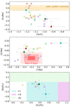 |
Fig. 15. Heavy-element enhancement diagnostic. Top panel: [Eu/Ba] versus [Fe/H] diagram for the four reference GCs. The Solar System r-process region is highlighted by the orange strip for [Eu/Ba] = +0.60 ± 0.13 (see text). Middle panel: [Zr/Ba] versus [Y/Ba] diagram for the three reference GCs that have Zr, Y, and Ba abundance determinations. The main r-process stars region is represented with the red-square (3 − σ). Bottom panel: [Ba/Eu] versus [Eu/Fe] diagram for the selected r-rich stars from the upper panel (see text). The light green region represents the regime of enhancement by both the r- and s-processes. The cyan and magenta regions show the domains of mainly r-process enhancement. The dot and cross colour code is the same as in Fig. 8. |
We also tentatively investigated the nature of heavy element enhancement through the diagnostic plots of Fig. 15 using the [Zr/Ba] ratio. The use of [Zr/Ba] as presented by Siqueira-Mello et al. (2016) consisted of using [Y/Ba] and values from the six r-rich halo stars compiled in Sneden et al. (2008), as representatives of the main r-process, which have a mean of [Y/Ba] = −0.42 ± 0.12. On the other hand, Siqueira-Mello et al. (2016) gathered another six halo metal-poor stars showing enhancement of the first peak of heavy elements, which have [Y/Ba] = +0.58 ± 0.18 on the other extreme. The same is applied to Zr-to-Ba, with [Zr/Ba] = −0.18 ± 0.12 and +0.95 ± 0.15 in the two extremes.
In the middle panel of Fig. 15, we show the [Zr/Ba] versus [Y/Ba] diagram for Pal 6 and three other reference bulge GCs. For diagnostics, we highlighted the region of main r-process stars (red region) at [Y/Ba]r = −0.4 ± 0.1 (Sneden et al. 2008) and [Zr/Ba]r = −0.2 ± 0.1 (Siqueira-Mello et al. 2016). Only three of the six observed stars are plotted due the absence of Ba abundance. The member stars 785 and 401 are consistent with r-rich stars considering the errors. Besides that, the star 401 is located at the highest star density; consequently, it is compatible with the reference GCs.
The bottom panel of Fig. 15 shows the further inspection of the r- and s-process to the r-rich stars selected by the [Eu/Ba] versus [Fe/H] and [Zr/Ba] versus [Y/Ba] diagrams. The two member stars (785 and 401) classified as r-rich are compatible with the definition of r-I, which is in agreement with that observed for the reference GCs.
4.10. Are there two stellar populations?
According to Martocchia et al. (2018, 2019), stellar clusters older than 2 Gyr show a presence of multiple stellar populations (MPs), evidenced by their chemical abundances. From a spectroscopic point of view, Osborn (1971) observed anomalous variations in carbon molecules in one star of M5 and another of M10. Later, Hartwick & McClure (1972) also discovered the anomaly in nitrogen. Currently, it is known that the phenomenon of MPs is also caused by star-by-star variations in light elements and helium mass fraction (Y) (Gratton et al. 2004, 2012; Carretta et al. 2010; Milone et al. 2018; Mészáros et al. 2020). Specifically, the major variation is in N with a maximum enrichment of δ[N/Fe]∼1.20 dex (Milone et al. 2018). For that reason, many works have sought N-enhanced stars in field stars and GCs as evidence of second-generation stars (e.g., Barbuy et al. 2016; Schiavon et al. 2017a; da Silveira et al. 2018; Fernández-Trincado et al. 2020, 2021).
It is important to determine whether the GC hosts MPs because this is related to the origin of the GC itself. For example, Bellini et al. (2017) analysed the complex Type II GC (Milone et al. 2017) ω−Cen (NGC 5139). They found that this cluster hosts at least five stellar populations, and that the populations can be split into 15 sub-populations. Their results show that ω−Cen is much more complex than the majority of GCs. Additionally, Massari et al. (2019) associated ω−Cen with the Gaia-Enceladus (Belokurov et al. 2018; Helmi et al. 2018) progenitor. This could be pointing to a cluster that originated from a merger event. However, ω−Cen seems to be more compatible with a core of a dwarf galaxy (Mészáros et al. 2021). For the ‘normal’ (Type I; Milone et al. 2017) GCs, we could expect them to have an origin from main components of the Galaxy, as observed in Massari et al. (2019) with 62 GCs associated with a so-called main-progenitor.
The expected N-O anti-correlation (Carretta et al. 2010; Gratton et al. 2004, 2012) is given in left panel of Fig. 16. We also found two N-rich non-member stars, which are possible field members, with [N/Fe] > +0.70. These could be stars that were Pal 6 or other cluster members trapped by the Galactic bulge (Schiavon et al. 2017b). Another indicator of MPs is the Na-O anti-correlation. Carretta et al. (2009a) demonstrated that this anti-correlation is more likely to be seen in massive clusters. Since Pal 6 is a relatively low-mass cluster (with an absolute magnitude of MV = −6.79; Harris 1996, 2010 edition), in Fig. 16 (right panel) we can observe a slight Na-O anti-correlation.
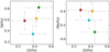 |
Fig. 16. Anti-correlations N-O (left) and Na-O (right) for Pal 6 member stars. |
To verify if our N-enhanced star 401 is a probable second-generation member, we investigated the Al-NaON relations (Fig. 17). Mészáros et al. (2020) analysed stars observed with the APOGEE for 31 GCs. They observed that at [Al/Fe] = +0.30, the stars are split reasonably well into two populations. We investigated these patterns and observed that our N-enhanced star has [Al/Fe] > +0.30, while the other three member stars have [Al/Fe] < +0.30. Even though the phenomenon of MPs (Bastian & Lardo 2018) is a characteristic of the majority of GCs (Piotto et al. 2015), Lagioia et al. (2019) presented the first evidence of a GC consistent with hosting a simple stellar population (Terzan 7). For that reason, the abundance pattern observed for Pal 6 is important in order to check if it hosts at least two stellar populations.
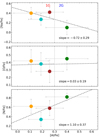 |
Fig. 17. Al-NaON (anti)correlations. The dots are coloured according to the same colour code of Fig. 16. The dotted grey line represents the generation split around [Al/Fe] = +0.30 (Mészáros et al. 2020). The black dashed lines show the obtained linear regression. |
5. Age and distance
Previous photometric studies did not attempt to derive the age of Pal 6, and there are controversies on its distance in the literature. These are largely due to the absence of observed standard candle stars in Pal 6, and different values result from different methods. Ortolani et al. (1995) derived a distance of ∼8.9 kpc from the horizontal branch (HB) magnitude method with an extinction of AV = 4.12. Lee & Carney (2002), comparing the Pal 6 HB magnitude to the 47 Tuc one, obtained a distance of ∼7.2 kpc with AV = 4.1 mag. Harris (1996) gave a distance of 5.80 kpc, which was adopted by Baumgardt et al. (2019) and used in Massari et al. (2019) and Pérez-Villegas et al. (2020).
With the final corrected CMD (Sect. 2.2), we used the SIRIUS code (Souza et al. 2020) to perform the statistical isochrone fitting to obtain the accurate probability distributions for the fundamental parameters of Pal 6. We employed isochrones from the MESA Isochrones & Stellar Tracks database (MIST; Dotter 2016; Choi et al. 2016) with the metallicity [Fe/H] ranging from 0.0 to −2.0 dex in steps of 0.01 dex and ages from 10 Gyr to 15 Gyr with an interval of 0.1 Gyr; the reddening and distance modulus can vary freely. To obtain a consistent analysis, we used a Gaussian prior for the metallicity with information from the high-resolution spectroscopic determination by this work.
We also obtained the temperature-dependent second-order extinction corrections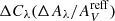 by comparing the MIST isochrones with AV = 0.00 and 6.0 for each value of Teff. The correction is given by the second-order polynomial function ΔCλ = a0 × (log Teff)2 + a1 × log Teff + a2, and the
  . As mentioned in Oliveira et al. (2020), the second-order correction is obtained by interpolation considering the desired AV. The coefficients a0, 1, 2 are listed in Table 9.
Coefficients for effective temperature second-order correction to different passbands.
We adopted the 50th percentile as the best solution and 50th − 16th and 84th − 50th percentiles for the uncertainties. The red line in Fig. 18 represents the best fit, while the red strip shows the region of 1 − σ solutions. We want to stress that the HB model fits well to the HB region in the CMD. Also, this technique allows us to obtain a better distance determination with low uncertainty. The best distance, reddening, and well-constrained metallicity values provided us with the first derivation of age for Pal 6 as 12.4 ± 0.9 Gyr, therefore it is among the oldest GCs in the Galaxy.
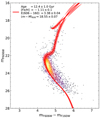 |
Fig. 18. Best-fit from isochrone fitting (solid line) and results for ±1σ (red region). |
The reddening E(606 − 160) = 3.38 ± 0.04 and distance modulus (m − M)606 = 18.55 ± 0.07 obtained from isochrone fitting can be converted in E(B − V) and (m − M)0 using the following relations:
 (2)
(2)
 (3)
(3)
where Cλ, RV is the ratio of temperature- and gravity-dependent coefficients at the λ for an extinction law with RV (Pallanca et al. 2021, and references therein). Since the extinction is given by Aλ = RV × Cλ, RV × E(B − V), the reddening is inversely proportional to RV. Therefore, the assumption of RV will affect the fundamental parameters of the cluster.
For the isochrone fitting, it is common to use the extinction law setting RV = 3.1, which is the case for all the fundamental parameters calculated for Pal 6 in the literature. With this extinction law, our determination is AV = 4.56 ± 0.06 (E(B − V)=1.47 ± 0.02), which is compatible with the reddening used to derive the photometric temperatures. However, Nataf et al. (2016) argue that a lower value of RV is more compatible with the Galactic bulge population, where it could reach down to RV = 2.5 at least for (absolute) Galactic latitudes between 2 and 7 degrees and −10° < l < 10°. Vasiliev & Baumgardt (2021) compared the distance from literature to the Gaia EDR3 parallaxes. They found a discrepancy between the photometric distances and the inverse of parallaxes for the bulge GCs, precisely those with high reddening values (E(B − V)> 1.0). Also, Pallanca et al. (2021) show that the RV = 3.1 needs different values of reddening and distance moduli to fit the CMD well with different colours in the case of the bulge GC Liller 1. They demonstrated that to fit the three CMDs simultaneously with a unique set of reddening and distance values, it is necessary to adopt an extinction law with RV = 2.5. They also conclude that the variation in the extinction law results in variations in the reddening and distance modulus determinations (consequently in the distance).
To determine the value of RV for Pal 6, we compare the optical (VI; Ortolani et al. 1995), GaiaGBP − GRP versus G, and NIR HST CMDs using the best-fit parameters of Fig. A.1. Since we varied the RV, we re-derived the extinction coefficients in the adopted bands (AF606W/AV, AF110W/AV, AF160W/AV, AGBP/AV, AGRP/AV, AG/AV, and AI/AV) using the extinction laws from Cardelli et al. (1989). The corresponding extinction law to a given RV value has been done by interpolating the curves in a grid with the values RV = 2.1, 3.1, 4, 5 (Fig. 19). We derived RV = 2.6 by maximising the negative χ2 for the optical and Gaia CMDs (first and second panels of Fig. 20). Finally, we determined an extinction of AV = 4.21 ± 0.05 (E(B − V)=1.62 ± 0.02) and a distance of d⊙ = 7.67 ± 0.19 kpc (Fig. 21), a result within the range between 5.8 kpc (Harris 1996, 2010) and 8.9 kpc (Ortolani et al. 1995) and very close to the Lee & Carney (2002) value of 7.2 kpc. We stress that the latter distance determination derived from near-IR JHK photometry is independent of the RV optical value.
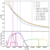 |
Fig. 19. Extinction law curves’ derivation. The effective wavelengths are computed from λeff = ∫λ2Tλdλ/∫λTλdλ. |
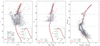 |
Fig. 20. Posterior fitting to obtain the best value of RV. First panel: optical CMD V − I versus I from Ortolani et al. (1995). Second panel: Gaia EDR3 GBP − GRP versus G CMD. Third panel: corrected NIR HST CMD. The cyan dotted lines are the isochrones considering the best fit from the standard isochrone fitting and standard extinction coefficient (RV = 3.0). The embedded plots show the χ2 function to the variation of RV. The solid red lines are the isochrones with the best RV value. Finally, the blue horizontal lines denote the isochrone HB and turn-off mean locus. |
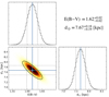 |
Fig. 21. New distance and reddening determinations using the best extinction law. |
To confirm our determination, we performed the distance calculation using two other methods. From the relation Mv−[Fe/H] derived by Oliveira et al. (2021) for RR Lyrae stars, we can obtain the HB absolute magnitude of 0.758 ± 0.086 in the V band. Assuming the apparent V-magnitude value of 19.70 ± 0.15 calculated for the HB of Pal 6 by Ortolani et al. (1995), we obtain the distance modulus of (m − M)V = 18.94 ± 0.18. Finally, with the extinction value found in the present work (AV = 4.21 ± 0.05, compatible with the average calculated with dust map of the Galaxy using the DUST web tool2), we have a distance of 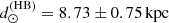 .
.
Using the Gaia EDR3 membership analysis (Sect. 2.3), we identified five stars with distances derived by the StarHorse calculations (with Gaia EDR3 and APOGEE DR16; Queiroz et al. 2020a, Queiroz et al. in prep). Due to the low statistics, we expanded the sample with a bootstrapping method taking into account the uncertainties. The mean distance derived from the expanded sample is 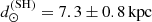 .
.
The individual distance determinations through the HB and StarHorse are already compatible within 1.5σ with our determination from the isochrone fitting of 7.67 ± 0.19 kpc. In addition, the average of these determinations results in a distance of ⟨d⊙⟩(HB,SH) = 8.0 ± 1.1 kpc, compatible with the distance of the present work. Finally, we added the average of the literature of 7.05 ± 0.46 kpc given by Baumgardt & Vasiliev (2021)
3, resulting in ⟨d⊙⟩(HB,SH,B\AMP V21) = 7.5 ± 1.0 kpc, which is in good agreement with our determination. Therefore, these results reinforce the one we found through the isochrone fitting of 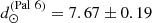 kpc calculated with the derived extinction law (RV = 2.6).
6. The origin of Pal 6
With the chemical information, age, and distance obtained in the previous sections, it is possible to infer a plausible origin of Pal 6. Using the distance of Harris (Harris 1996), which was adopted by Baumgardt et al. (2019), Pérez-Villegas et al. (2020) classified Pal 6 as belonging to the Galaxy thick disc with a probability of 98%. Caution was recommended given other distance estimations in the literature (e.g., Ortolani et al. 1995).
Given the much more reliable distance now derived in the present paper, we carried out the calculations of orbits for the cluster. We employed the same Galactic model of Pérez-Villegas et al. (2018, 2020) that includes a triaxial Ferrers bar of 3.5 kpc (major axis). The total mass of the bar is 1.2 × 10¹⁰ M⊙, with an angle of 25° with the Sun-major axis. We also assume three pattern speeds of the bar: Ωb = 40, 45, and 50 km s−1 kpc−1.
We generated a set of 1000 initial conditions employing a Monte Carlo approach. In order to do that, we considered the observational uncertainties of distance, heliocentric radial velocity, and absolute proper motion components, with the purpose of evaluating the errors in those observational parameters. We integrated the orbits forward for 10 Gyr using the NIGO tool (Rossi 2015). In Table 10, we give the new orbital parameters as the median values of the perigalactic distance ⟨rmin⟩, apogalactic distance ⟨rmax⟩, mean eccentricity ⟨e⟩ (where the eccentricity is defined as e = (rmax − rmin)/(rmax + rmin)), and maximum vertical excursion from the Galactic plane ⟨|z|max⟩. The error of each orbital parameter is given as the standard deviation of the distribution.
Orbital parameters of Pal 6 for the McMillan (2017) potential and the potential employed in Pérez-Villegas et al. (2020) assuming three different bar pattern speed values.
In Fig. 22, we show the probability density map of the orbits of Pal 6 in the x − y and R − z projections co-rotating with the bar. The gold colour displays the space region that the orbits of Pal 6 cross more frequently, while the black curves are the orbits considering the central values of the observational parameters. We can observe that Pal 6 is mostly confined within ∼2.1 kpc, and therefore has a high probability of belonging to the bulge component (> 99%), when we adopt the distance of 7.67 kpc estimated in this work. Our new distance determination points out that Pal 6 is also a very inner cluster due to its maximum height of |z|< 1.3 kpc and a high eccentric orbit. Those characteristics were also found for the GCs NGC 6522, NGC 6558, and HP 1, which are very old and moderately metal-poor GCs of the Galactic bulge.
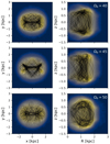 |
Fig. 22. Probability density map for the x − y and R − z projections of the set of orbits for Pal 6 using three different values of Ωb = 40, 45, and 50 km s−1 kpc−1. The orbits are co-rotating with the bar frame. The gold colour corresponds to the higher probabilities, while the black lines show the orbits using the central observational parameters. |
Based on our analysis, we are confident that Pal 6 is confined within the Galactic bulge. However, it remains unclear if this cluster is originated from the Galaxy or due to some merger process that occurred in the early stages of the Milky Way. To elucidate whether Pal 6 was formed in situ or accreted, we followed the method described in Massari et al. (2019) to determine the probable progenitor of Pal 6. The classification is based on the integrals of motion space Lz and E, and the age-metallicity relation (AMR). It is important to mention that these integrals of motion are only conserved by Galactic potential in an axisymmetric model. Because of that, we employed the axisymmetric potential of McMillan (2017) and recalculated the orbital parameters of Pal 6 using the python-package galpy (Bovy 2015). For this case, we also integrated forward for 10 Gyr and employed a set of 1000 initial conditions. The reason for adopting the McMillan (2017) Galactic potential is to compare our results with Massari et al. (2019) and to relate Pal 6 with its plausible progenitor. The orbital parameters with the axisymmetric potential are listed in last column of Table 10.
We found Lz = 7.88 ± 13.22 km s−1 kpc and E = (−2.40±0.05) × 105 km2 s−2. Pal 6 is compatible with three progenitors due to its low values of E, Lz, and z-perpendicular angular momentum Lperp (see Fig. 23): the main progenitor (in situ), a low-energy progenitor (low-energy), and Gaia-Enceladus. Massari et al. (2019) classified Pal 6 as having been formed by the low-energy progenitor due to the previous values of distance employed. Since the classification of a main-bulge progenitor is related to the apogalactic distance rmax < 3.6 kpc (maximum 3D radius of the orbit), Pal 6 is clearly compatible with this definition.
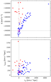 |
Fig. 23. Integrals of motion space of 82 Galactic GCs. The colour-code relates to the association with their probable progenitor (Massari et al. 2019); Gaia-Enceladus is marked in red, low-energy in pink, and the main progenitor in blue. The magenta square represents Pal 6 with the values of the present work. |
On the other hand, with our new determination of [Fe/H] from high-resolution spectroscopy and the age derivation of Pal 6, we can observe the location of the cluster in the AMRs. Figure 24 shows the AMRs for the clusters according to its associated progenitors for the ones more compatible with Pal 6. We found that Pal 6 is located in a possible ridge line of the main-progenitor distribution. Therefore, according to the classification of the present work, in combination with the classifications presented in Massari et al. (2019), we conclude that Pal 6 is a cluster of the Galactic bulge having been formed in situ.
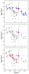 |
Fig. 24. Age-metallicity relation (AMR) for 82 GCs (black dots) analysed by Massari et al. (2019) (plot based on their Fig. 4). The ages are taken from Vandenberg et al. (2013) and the metallicities from Carretta et al. (2009b). In each panel, one progenitor is highlighted. From top to bottom: First panel, main-progenitor (disc and bulge); second panel, low energy; third panel, Gaia-Enceladus. The magenta square represents Pal 6 with metallicity and age of the present work. |
This result could also give us an explanation about the possible formation scenario of the MPs in Pal 6. Since the cluster was formed in situ, the most compatible formation scenarios of MPs are those predicted by internal pollution of the cluster. This hypothesis is in agreement with the results described in the chemical abundances of heavy elements found in this work. A more detailed analysis of the stellar ages is required to provide a constraint on the most probable formation scenario (Nardiello et al. 2015; Souza et al. 2020; Oliveira et al. 2020; Lucertini et al. 2021).
7. Conclusions
We present a complete and detailed analysis of the GC Pal 6, through the analysis of high-resolution spectra of the UVES spectrograph, HST photometry, and a dynamical analysis. Based on Gaia EDR3, we determined that four of our six sample stars are members of Pal 6 and give a heliocentric radial velocity consistent with values from the literature.
With the UVES spectroscopic data, we determined the final stellar parameters and abundances for the six sample stars. The metallicity of [Fe/H] = −1.10 ± 0.09 and α-element enhancement of [α/Fe] = +0.35 ± 0.06 were derived. One of the member stars is N-enhanced, indicating a presence of second-generation stars, confirmed from a separation into two populations based on a [Al/Fe] = +0.30 threshold. We can also observe that the abundance pattern of Pal 6 is very similar in many aspects to the GCs typical of the bulge population such as NGC 6266 (M 62; Yong et al. 2014), HP 1 (Barbuy et al. 2016), NGC 6558 (Barbuy et al. 2018a), and NGC 6522 (Barbuy et al. 2014, Barbuy et al. 2021), as illustrated in Fig. 25. The Si, Ca, and Ti abundances are also low enhanced. The abundances of the first-peak of heavy elements are relatively high, while the second-peak of heavy elements is moderately high. Finally, the r-element Eu is enhanced. It is interesting to note that the four reference bulge GCs are representatives of moderately metal-poor GCs with a BHB, whereas Pal 6 has an RHB.
 |
Fig. 25. Abundance pattern [X/Fe] vs. atomic number (Z) of the references moderately metal-poor bulge GCs NGC 6558, NGC 6522, M62, and HP 1. The colours are the same as Fig. 8. |
A photometric analysis combined with dynamics was performed in order to determine the probable progenitor of the cluster. For this, we derived an age of 12.4 ± 0.9 Gyr and a distance of 7.67 ± 0.19 kpc. Due to the new and more reliable distance value, the orbital analysis indicates that Pal 6 is confined within the Galactic bulge. The dynamical analysis and the values of the age and metallicity of Pal 6 show that the cluster was most probably formed in the main-bulge progenitor of the Galaxy (in situ). Finally, considering that Pal 6 was formed in the Galaxy, it is probable that the second generation of stars in the cluster could be formed from internal pollution of the cluster, which is compatible with both the AGB star (Renzini et al. 2015; Calura et al. 2019) and fast-rotating massive star (Decressin et al. 2007; Chiappini et al. 2011; Frischknecht et al. 2016) pollution scenarios.
The study of GCs is of great importance to understand the formation and evolution of the Galaxy. Our analysis shows that Pal 6 is a GC formed in the Galactic bulge progenitor present in the early stages of the Milky Way, and it shares chemical properties with other well-known old-bulge GCs.
They considered the distances from Ortolani et al. (1995), Barbuy et al. (1998), Lee & Carney (2002), and Lee et al. (2004). Because of the expected distance for Pal 6, they did not consider the inverse of the parallax given by Vasiliev & Baumgardt (2021).
Acknowledgments
We acknowledge our referee, Dr. Thomas Masseron, for the detailed review and for the helpful suggestions, which allowed us to improve the manuscript. We are grateful to Anna B. A. Queiroz for providing the StarHorse distances with APOGEE DR16 and Gaia EDR3. SOS acknowledges the FAPESP PhD fellowship 2018/22044-3. S. O. S. and A. P. V. acknowledge the DGAPA-PAPIIT grant IG100319. B. B. and E. B. acknowledge grants from FAPESP, CNPq and CAPES – Financial code 001. S. O. acknowledges the partial support of the research program DOR1901029, 2019, and the project BIRD191235, 2019 of the University of Padova. M. V. acknowledges the support of the Deutsche Forschungsgemeinschaft (DFG, project number: 428473034). Part of this work was supported by the German Deutsche Forschungsgemeinschaft, DFG project number Ts 17/2–1. DN acknowledges the support from the French Centre National d’Etudes Spatiales (CNES).
References
- Alonso, A., Arribas, S., & Martínez-Roger, C. 1999, A&AS, 140, 261 [NASA ADS] [CrossRef] [EDP Sciences] [Google Scholar]
- Ballester, P., Modigliani, A., Boitquin, O., et al. 2000, Messenger, 101, 31 [NASA ADS] [Google Scholar]
- Barbuy, B., Bica, E., & Ortolani, S. 1998, A&A, 333, 117 [NASA ADS] [Google Scholar]
- Barbuy, B., Chiappini, C., Cantelli, E., et al. 2014, A&A, 570, A76 [NASA ADS] [CrossRef] [EDP Sciences] [Google Scholar]
- Barbuy, B., Cantelli, E., Vemado, A., et al. 2016, A&A, 591, A53 [NASA ADS] [CrossRef] [EDP Sciences] [Google Scholar]
- Barbuy, B., Chiappini, C., & Gerhard, O. 2018a, ARA&A, 56, 223 [Google Scholar]
- Barbuy, B., Muniz, L., Ortolani, S., et al. 2018b, A&A, 619, A178 [NASA ADS] [CrossRef] [EDP Sciences] [Google Scholar]
- Barbuy, B., Trevisan, J., & de Almeida, A. 2018c, PASA, 35, 46 [Google Scholar]
- Barbuy, B., Cantelli, E., Muniz, L., et al. 2021, A&A, 654, A29 [NASA ADS] [CrossRef] [EDP Sciences] [Google Scholar]
- Bastian, N., & Lardo, C. 2018, ARA&A, 56, 83 [Google Scholar]
- Baumgardt, H., & Vasiliev, E. 2021, MNRAS, 505, 5957 [NASA ADS] [CrossRef] [Google Scholar]
- Baumgardt, H., Hilker, M., Sollima, A., et al. 2019, MNRAS, 482, 5138 [NASA ADS] [CrossRef] [Google Scholar]
- Beers, T. C., & Christlieb, N. 2005, ARA&A, 43, 531 [NASA ADS] [CrossRef] [Google Scholar]
- Bellini, A., Piotto, G., Bedin, L. R., et al. 2009, A&A, 493, 959 [NASA ADS] [CrossRef] [EDP Sciences] [Google Scholar]
- Bellini, A., Milone, A. P., Anderson, J., et al. 2017, ApJ, 844, 164 [NASA ADS] [CrossRef] [Google Scholar]
- Belokurov, V., Erkal, D., Evans, N. W., et al. 2018, MNRAS, 478, 611 [NASA ADS] [CrossRef] [Google Scholar]
- Bica, E., Ortolani, S., & Barbuy, B. 2016, PASA, 33, e028 [Google Scholar]
- Bovy, J. 2015, ApJS, 216, 29 [NASA ADS] [CrossRef] [Google Scholar]
- Calura, F., D’Ercole, A., Vesperini, E., et al. 2019, MNRAS, 489, 3269 [NASA ADS] [Google Scholar]
- Cardelli, J. A., Clayton, G. C., & Mathis, J. S. 1989, ApJ, 345, 245 [Google Scholar]
- Carretta, E., Bragaglia, A., Gratton, R., et al. 2009a, A&A, 508, 695 [NASA ADS] [CrossRef] [EDP Sciences] [Google Scholar]
- Carretta, E., Bragaglia, A., Gratton, R., et al. 2009b, A&A, 505, 139 [NASA ADS] [CrossRef] [EDP Sciences] [Google Scholar]
- Carretta, E., Bragaglia, A., Gratton, R. G., et al. 2010, A&A, 516, A55 [NASA ADS] [CrossRef] [EDP Sciences] [Google Scholar]
- Casagrande, L., Ramírez, I., Meléndez, J., et al. 2010, A&A, 512, A54 [NASA ADS] [CrossRef] [EDP Sciences] [Google Scholar]
- Cayrel, R., Depagne, E., Spite, M., et al. 2004, A&A, 416, 1117 [NASA ADS] [CrossRef] [EDP Sciences] [Google Scholar]
- Cescutti, G., Chiappini, C., Hirschi, R., et al. 2013, A&A, 553, A51 [NASA ADS] [CrossRef] [EDP Sciences] [Google Scholar]
- Cescutti, G., Romano, D., Matteucci, F., et al. 2015, A&A, 577, A139 [NASA ADS] [CrossRef] [EDP Sciences] [Google Scholar]
- Chiappini, C., Frischknecht, U., Meynet, G., et al. 2011, Nature, 474, 666 [NASA ADS] [CrossRef] [Google Scholar]
- Choi, J., Dotter, A., Conroy, C., et al. 2016, ApJ, 823, 102 [Google Scholar]
- Choplin, A., Hirschi, R., Meynet, G., et al. 2018, A&A, 618, A133 [NASA ADS] [CrossRef] [EDP Sciences] [Google Scholar]
- Coelho, P., Barbuy, B., Meléndez, J., et al. 2005, A&A, 443, 735 [NASA ADS] [CrossRef] [EDP Sciences] [Google Scholar]
- Cohen, R. E., Mauro, F., Alonso-García, J., et al. 2018, AJ, 156, 41 [Google Scholar]
- da Silveira, C. R., Barbuy, B., Friaça, A. C. S., et al. 2018, A&A, 614, A149 [NASA ADS] [CrossRef] [EDP Sciences] [Google Scholar]
- Decressin, T., Meynet, G., Charbonnel, C., et al. 2007, A&A, 464, 1029 [NASA ADS] [CrossRef] [EDP Sciences] [Google Scholar]
- Dias, B., Barbuy, B., Saviane, I., et al. 2016, A&A, 590, A9 [NASA ADS] [CrossRef] [EDP Sciences] [Google Scholar]
- Dotter, A. 2016, ApJs, 222, 8 [NASA ADS] [CrossRef] [Google Scholar]
- Ernandes, H., Barbuy, B., Alves-Brito, A., et al. 2018, A&A, 616, A18 [NASA ADS] [CrossRef] [EDP Sciences] [Google Scholar]
- Fernández-Trincado, J. G., Minniti, D., Beers, T. C., et al. 2020, A&A, 643, A145 [Google Scholar]
- Fernández-Trincado, J. G., Minniti, D., Souza, S. O., et al. 2021, ApJ, 908, L42 [Google Scholar]
- Frischknecht, U., Hirschi, R., Pignatari, M., et al. 2016, MNRAS, 456, 1803 [Google Scholar]
- Gaia Collaboration (Brown, A. G. A., et al.) A&A, 649, A1 [Google Scholar]
- Gratton, R., Sneden, C., & Carretta, E. 2004, ARA&A, 42, 385 [Google Scholar]
- Gratton, R. G., Carretta, E., & Bragaglia, A. 2012, A& Arv, 20, 50 [Google Scholar]
- Grevesse, N., & Sauval, A. J. 1998, Space Sci. Rev., 85, 161 [Google Scholar]
- Grevesse, N., Scott, P., Asplund, M., et al. 2015, A&A, 573, A27 [NASA ADS] [CrossRef] [EDP Sciences] [Google Scholar]
- Gustafsson, B., Edvardsson, B., Eriksson, K., et al. 2008, A&A, 486, 951 [NASA ADS] [CrossRef] [EDP Sciences] [Google Scholar]
- Harris, W. E. 1996, AJ, 112, 1487 [Google Scholar]
- Hartwick, F. D. A., & McClure, R. D. 1972, ApJ, 176, L57 [NASA ADS] [CrossRef] [Google Scholar]
- Helmi, A., & de Zeeuw, P. T. 2000, MNRAS, 319, 657 [Google Scholar]
- Helmi, A., Babusiaux, C., Koppelman, H. H., et al. 2018, Nature, 563, 85 [Google Scholar]
- Hinkle, K., Wallace, L., Valenti, J., & Harmer, D. 2000, in Visible and Near Infrared Atlas of the Arcturus Spectrum 3727–9300 Å, eds. K. Hinkle, L. Wallace, J. Valenti, & D. Harmer (San Francisco: ASP) [Google Scholar]
- Howell, S. B., Sobeck, C., Haas, M., et al. 2014, PASP, 126, 398 [Google Scholar]
- Kerber, L. O., Libralato, M., Souza, S. O., et al. 2019, MNRAS, 484, 5530 [Google Scholar]
- Kunder, A., Crabb, R. E., Debattista, V. P., et al. 2021, AJ, 162, 86 [NASA ADS] [CrossRef] [Google Scholar]
- Lagioia, E. P., Milone, A. P., Marino, A. F., et al. 2019, AJ, 158, 202 [NASA ADS] [CrossRef] [Google Scholar]
- Lee, J.-W., & Carney, B. W. 2002, AJ, 123, 3305 [NASA ADS] [CrossRef] [Google Scholar]
- Lee, J.-W., Carney, B. W., & Balachandran, S. C. 2004, AJ, 128, 2388 [NASA ADS] [CrossRef] [Google Scholar]
- Lucertini, F., Nardiello, D., & Piotto, G. 2021, A&A, 646, A125 [NASA ADS] [CrossRef] [EDP Sciences] [Google Scholar]
- McMillan, P. J. 2017, MNRAS, 465, 76 [NASA ADS] [CrossRef] [Google Scholar]
- Malkan, M. A. 1981, IAU Colloq. 68: Astrophysical Parameters for Globular Clusters, 533 [Google Scholar]
- Martín, E. L., Basri, G., Pavlenko, Y., et al. 2002, ApJ, 579, 437 [CrossRef] [Google Scholar]
- Martocchia, S., Cabrera-Ziri, I., Lardo, C., et al. 2018, MNRAS, 473, 2688 [NASA ADS] [CrossRef] [Google Scholar]
- Martocchia, S., Dalessandro, E., Lardo, C., et al. 2019, MNRAS, 487, 5324 [Google Scholar]
- Massari, D., Koppelman, H. H., & Helmi, A. 2019, A&A, 630, L4 [NASA ADS] [CrossRef] [EDP Sciences] [Google Scholar]
- Meléndez, J., & Barbuy, B. 2009, A&A, 497, 611 [NASA ADS] [CrossRef] [EDP Sciences] [Google Scholar]
- Mészáros, S., Masseron, T., García-Hernández, D. A., et al. 2020, MNRAS, 492, 1641 [Google Scholar]
- Mészáros, S., Masseron, T., Fernández-Trincado, J. G., et al. 2021, MNRAS, 505, 1645 [Google Scholar]
- Miglio, A., Chaplin, W. J., Brogaard, K., et al. 2016, MNRAS, 461, 760 [NASA ADS] [CrossRef] [Google Scholar]
- Milone, A. P., Piotto, G., Bedin, L. R., et al. 2012, A&A, 540, A16 [NASA ADS] [CrossRef] [EDP Sciences] [Google Scholar]
- Milone, A. P., Piotto, G., Renzini, A., et al. 2017, MNRAS, 464, 3636 [Google Scholar]
- Milone, A. P., Marino, A. F., Renzini, A., et al. 2018, MNRAS, 481, 5098 [NASA ADS] [CrossRef] [Google Scholar]
- Modigliani, A., Mulas, G., Porceddu, I., et al. 2004, Messenger, 118, 8 [NASA ADS] [Google Scholar]
- Nardiello, D., Piotto, G., Milone, A. P., et al. 2015, MNRAS, 451, 312 [NASA ADS] [CrossRef] [Google Scholar]
- Nardiello, D., Libralato, M., Piotto, G., et al. 2018, MNRAS, 481, 3382 [NASA ADS] [CrossRef] [Google Scholar]
- Nataf, D. M., Gonzalez, O. A., Casagrande, L., et al. 2016, MNRAS, 456, 2692 [Google Scholar]
- Oliveira, R. A. P., Souza, S. O., Kerber, L. O., et al. 2020, ApJ, 891, 37 [Google Scholar]
- Oliveira, R. A. P., Ortolani, S., Barbuy, B., et al. 2021, arXiv eprints [arXiv:2110.13943] [Google Scholar]
- Ortolani, S., Bica, E., & Barbuy, B. 1995, A&A, 296, 680 [NASA ADS] [Google Scholar]
- Ortolani, S., Held, E. V., Nardiello, D., et al. 2019, A&A, 627, A145 [NASA ADS] [CrossRef] [EDP Sciences] [Google Scholar]
- Osborn, W. 1971, Observatory, 91, 223 [Google Scholar]
- Pallanca, C., Lanzoni, B., Ferraro, F. R., et al. 2021, ApJ, 913, 137 [NASA ADS] [CrossRef] [Google Scholar]
- Pedregosa, F., Varoquaux, G., Gramfort, A., et al. 2011, JMLR, 12, 2825 [Google Scholar]
- Pérez-Villegas, A., Rossi, L., Ortolani, S., et al. 2018, PASA, 35 [Google Scholar]
- Pérez-Villegas, A., Barbuy, B., Kerber, L. O., et al. 2020, MNRAS, 491, 3251 [Google Scholar]
- Piotto, G., Milone, A. P., Bedin, L. R., et al. 2015, AJ, 149, 91 [Google Scholar]
- Piskunov, N. E., Kupka, F., Ryabchikova, T. A., et al. 1995, A&As, 112, 525 [Google Scholar]
- Queiroz, A. B. A., Anders, F., Chiappini, C., et al. 2020a, A&A, 638, A76 [NASA ADS] [CrossRef] [EDP Sciences] [Google Scholar]
- Queiroz, A. B. A., Chiappini, C., Pérez-Villegas, A., et al. 2020b, A&A, submitted, [arXiv:2007.12915] [Google Scholar]
- Renzini, A., D’Antona, F., Cassisi, S., et al. 2015, MNRAS, 454, 4197 [Google Scholar]
- Riello, M., De Angeli, F., Evans, D. W., et al. 2021, A&A, 649, A3 [NASA ADS] [CrossRef] [EDP Sciences] [Google Scholar]
- Rojas-Arriagada, A., Zasowski, G., Schultheis, M., et al. 2020, MNRAS, 499, 1037 [Google Scholar]
- Rossi, L. J. 2015, Astron. Comput., 12, 11 [Google Scholar]
- Ryabchikova, T., Piskunov, N., Kurucz, R. L., et al. 2015, PhyS, 90, 054005 [Google Scholar]
- Saito, R. K., Hempel, M., Minniti, D., et al. 2012, A&A, 537, A107 [NASA ADS] [CrossRef] [EDP Sciences] [Google Scholar]
- Schiavon, R. P., Zamora, O., Carrera, R., et al. 2017a, MNRAS, 465, 501 [Google Scholar]
- Schiavon, R. P., Johnson, J. A., Frinchaboy, P. M., et al. 2017b, MNRAS, 466, 1010 [NASA ADS] [CrossRef] [Google Scholar]
- Skrutskie, M. F., Cutri, R. M., Stiening, R., et al. 2006, AJ, 131, 1163 [NASA ADS] [CrossRef] [Google Scholar]
- Simmerer, J., Sneden, C., Cowan, J. J., et al. 2004, ApJ, 617, 1091 [Google Scholar]
- Siqueira-Mello, C., Chiappini, C., Barbuy, B., et al. 2016, A&A, 593, A79 [NASA ADS] [CrossRef] [EDP Sciences] [Google Scholar]
- Sneden, C., Cowan, J. J., & Gallino, R. 2008, ARA&A, 46, 241 [Google Scholar]
- Soto, M., Barbá, R., Gunthardt, G., et al. 2013, A&A, 552, A101 [NASA ADS] [CrossRef] [EDP Sciences] [Google Scholar]
- Souza, S. O., Kerber, L. O., Barbuy, B., et al. 2020, ApJ, 890, 38 [Google Scholar]
- Stassun, K. G., Oelkers, R. J., Pepper, J., et al. 2018, AJ, 156, 102 [Google Scholar]
- Stetson, P. B., & Pancino, E. 2008, PASP, 120, 1332 [Google Scholar]
- Truran, J. W. 1981, A&A, 97, 391 [NASA ADS] [Google Scholar]
- Tumlinson, J. 2010, ApJ, 708, 1398 [CrossRef] [Google Scholar]
- Vandenberg, D. A., Brogaard, K., Leaman, R., & Casagrande, L. 2013, ApJ, 775, 134 [Google Scholar]
- Vasiliev, E., & Baumgardt, H. 2021, MNRAS, 505, 5978 [NASA ADS] [CrossRef] [Google Scholar]
- Yong, D., Alves Brito, A., Da Costa, G. S., et al. 2014, MNRAS, 439, 2638 [NASA ADS] [CrossRef] [Google Scholar]
- Wise, J. H., Turk, M. J., Norman, M. L., et al. 2012, ApJ, 745, 50 [NASA ADS] [CrossRef] [Google Scholar]
Appendix A: Fundamental parameter determination
Figure A.1 shows the corner plots, which represent the 4D parameter space of the isochrone fitting (age, reddening, distance modulus, and metallicity) represented in 2D density distributions. The cumulative best solutions (posterior distributions) of each parameter are represented by the histograms, while the 2D density maps show the correlations between the parameters. To represent the distributions of each parameter, we assumed the region of highest density as the representative value, and the uncertainties were calculated from the 16th and 84th percentiles.
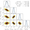 |
Fig. A.1. Corner plots with the parameter correlations. |
Appendix B: Line list
Equivalent widths for Fe I and Fe II lines.
Line-by-line abundance ratios in the six UVES sample stars for the CNO, odd-Z (Na and Al), alpha- (Mg, Si, Ca, and Ti), and heavy elements (Y, Zr, Ba, La, and Eu).
All Tables
Log of the spectroscopic FLAMES-UVES observations of programme 0103.D-0828 (A), carried out in 2019.
Radial velocity obtained for each extracted spectra and the average value for each star.
Identifications, coordinates, and magnitudes. JHKs are given from both 2MASS and VVV surveys.
Atmospheric parameters derived from photometry using calibrations by Casagrande et al. (2010) for V − I, V − K, J − K, and spectroscopic analysis of Fe lines.
Carbon, nitrogen, and oxygen abundances [X/Fe] from C2, CN bandheads, and [OI], respectively.
Sensitivity in abundances due to variation in atmospheric parameters for the star 243, considering uncertainties of ΔTeff = 100 K and Δlog g = 0.2, Δvt = 0.2 km s−1.
Coefficients for effective temperature second-order correction to different passbands.
Orbital parameters of Pal 6 for the McMillan (2017) potential and the potential employed in Pérez-Villegas et al. (2020) assuming three different bar pattern speed values.
Line-by-line abundance ratios in the six UVES sample stars for the CNO, odd-Z (Na and Al), alpha- (Mg, Si, Ca, and Ti), and heavy elements (Y, Zr, Ba, La, and Eu).
All Figures
|
Fig. 1. JHKs-combined colour image from the VVV survey for Pal 6. The image has a size of 2 × 2 arcmin2. North is at 45°anticlockwise. |
| In the text | |
|
Fig. 2. Procedure to obtain the photometry of Pal 6. First panel: HST photometry from Cohen et al. (2018). Second panel: stars selected by the quality method within a radius of ∼0.66 arcmin from the cluster centre. Third panel: differential reddening corrected CMD. Last panel: differential reddening map. |
| In the text | |
|
Fig. 3. Proper motion analysis to obtain the cluster members. Top left panel: sky distribution of stars within 10 arcmin of the cluster centre. Bottom left panel: vector point diagram with the cluster (coloured dots) and field (grey dots) stars; the green star symbols are the observed stars with FLAMES-UVES, and the insert plots show the density distributions found using GMMs. Right panel: Gaia EDR3 G versus GBP − GRP CMD; the green star symbols are the observed stars. From the bottom left and right panels, we can identify that two observed stars have zero membership probability (yellow star symbols). |
| In the text | |
|
Fig. 4. Excitation and ionisation equilibria of Fe I and Fe II lines for the four member stars. The black dots are the values considered to compute the metallicity of Fe I lines after a sigma-clipping of 1 − σ. The crosses are the omitted values. The red squares are the values of Fe II lines. The α values show the slope of the trends of Fe I lines. |
| In the text | |
|
Fig. 5. Fit to Y I 6435.004 Å line for star 243. The red dotted lines are the synthetic spectra, the blue strip represents the 1σ region, and the observed spectrum is the black solid line. The values of χ2 are in the insert plot. |
| In the text | |
|
Fig. 6. Example for star 243 line fit of the bandhead C2(0,1) (left) and [OI] (right). The solid cyan line is the best-fit abundance ratio, while the dotted lines consider [X/Fe] = [X/Fe]best ± 0.20 (red, plus – blue, minus). |
| In the text | |
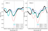 |
Fig. 7. Same as Fig. 6, but for N from CN(5,1) (left) and CN(6,2) (right). |
| In the text | |
|
Fig. 8. Odd-Z elements, Na (top panel) and Al (bottom panel), abundances as a function of metallicity [Fe/H]. Symbols: Crosses correspond to M 62 (gold; Yong et al. 2014), NGC 6558 (red; Barbuy et al. 2018b), NGC 6552 (green; Barbuy et al. 2021), and HP 1 (purple; Barbuy et al. 2016). The pink square shows the mean value of Pal 6. The filled dots are the mean abundances, together with the error bars. |
| In the text | |
|
Fig. 9. Same as Fig. 6, but for α−elements Mg (top left) Si (top right), Ca (bottom left), and Ti (bottom right). |
| In the text | |
|
Fig. 10. α−elements Mg (top panel) and Si (bottom panel) as functions of metallicity [Fe/H]. The colour code is the same in Fig. 8. |
| In the text | |
|
Fig. 11. α−elements Ca (top panel) and Ti (bottom panel) as functions of metallicity [Fe/H]. The colour code is the same in Fig. 8. |
| In the text | |
|
Fig. 12. Same as Fig. 6, but for heavy elements Y (top left), Ba (top right), La (bottom left), and Eu (bottom right). |
| In the text | |
|
Fig. 13. Heavy-elements Y (top panel) and Ba (bottom panel) as a functions of metallicity [Fe/H]. The colour code is the same as in Fig. 8. |
| In the text | |
|
Fig. 14. Heavy-elements La (top panel) and Eu (bottom panel) as functions of metallicity [Fe/H]. The colour code is the same as in Fig. 8. |
| In the text | |
|
Fig. 15. Heavy-element enhancement diagnostic. Top panel: [Eu/Ba] versus [Fe/H] diagram for the four reference GCs. The Solar System r-process region is highlighted by the orange strip for [Eu/Ba] = +0.60 ± 0.13 (see text). Middle panel: [Zr/Ba] versus [Y/Ba] diagram for the three reference GCs that have Zr, Y, and Ba abundance determinations. The main r-process stars region is represented with the red-square (3 − σ). Bottom panel: [Ba/Eu] versus [Eu/Fe] diagram for the selected r-rich stars from the upper panel (see text). The light green region represents the regime of enhancement by both the r- and s-processes. The cyan and magenta regions show the domains of mainly r-process enhancement. The dot and cross colour code is the same as in Fig. 8. |
| In the text | |
|
Fig. 16. Anti-correlations N-O (left) and Na-O (right) for Pal 6 member stars. |
| In the text | |
|
Fig. 17. Al-NaON (anti)correlations. The dots are coloured according to the same colour code of Fig. 16. The dotted grey line represents the generation split around [Al/Fe] = +0.30 (Mészáros et al. 2020). The black dashed lines show the obtained linear regression. |
| In the text | |
|
Fig. 18. Best-fit from isochrone fitting (solid line) and results for ±1σ (red region). |
| In the text | |
|
Fig. 19. Extinction law curves’ derivation. The effective wavelengths are computed from λeff = ∫λ2Tλdλ/∫λTλdλ. |
| In the text | |
|
Fig. 20. Posterior fitting to obtain the best value of RV. First panel: optical CMD V − I versus I from Ortolani et al. (1995). Second panel: Gaia EDR3 GBP − GRP versus G CMD. Third panel: corrected NIR HST CMD. The cyan dotted lines are the isochrones considering the best fit from the standard isochrone fitting and standard extinction coefficient (RV = 3.0). The embedded plots show the χ2 function to the variation of RV. The solid red lines are the isochrones with the best RV value. Finally, the blue horizontal lines denote the isochrone HB and turn-off mean locus. |
| In the text | |
|
Fig. 21. New distance and reddening determinations using the best extinction law. |
| In the text | |
|
Fig. 22. Probability density map for the x − y and R − z projections of the set of orbits for Pal 6 using three different values of Ωb = 40, 45, and 50 km s−1 kpc−1. The orbits are co-rotating with the bar frame. The gold colour corresponds to the higher probabilities, while the black lines show the orbits using the central observational parameters. |
| In the text | |
|
Fig. 23. Integrals of motion space of 82 Galactic GCs. The colour-code relates to the association with their probable progenitor (Massari et al. 2019); Gaia-Enceladus is marked in red, low-energy in pink, and the main progenitor in blue. The magenta square represents Pal 6 with the values of the present work. |
| In the text | |
|
Fig. 24. Age-metallicity relation (AMR) for 82 GCs (black dots) analysed by Massari et al. (2019) (plot based on their Fig. 4). The ages are taken from Vandenberg et al. (2013) and the metallicities from Carretta et al. (2009b). In each panel, one progenitor is highlighted. From top to bottom: First panel, main-progenitor (disc and bulge); second panel, low energy; third panel, Gaia-Enceladus. The magenta square represents Pal 6 with metallicity and age of the present work. |
| In the text | |
|
Fig. 25. Abundance pattern [X/Fe] vs. atomic number (Z) of the references moderately metal-poor bulge GCs NGC 6558, NGC 6522, M62, and HP 1. The colours are the same as Fig. 8. |
| In the text | |
|
Fig. A.1. Corner plots with the parameter correlations. |
| In the text | |
Current usage metrics show cumulative count of Article Views (full-text article views including HTML views, PDF and ePub downloads, according to the available data) and Abstracts Views on Vision4Press platform.
Data correspond to usage on the plateform after 2015. The current usage metrics is available 48-96 hours after online publication and is updated daily on week days.
Initial download of the metrics may take a while.