| Issue |
A&A
Volume 654, October 2021
|
|
|---|---|---|
| Article Number | A51 | |
| Number of page(s) | 20 | |
| Section | The Sun and the Heliosphere | |
| DOI | https://doi.org/10.1051/0004-6361/202141404 | |
| Published online | 08 October 2021 | |
Evidence of the multi-thermal nature of spicular downflows
Impact on solar atmospheric heating⋆
1
Institute of Theoretical Astrophysics, University of Oslo, PO Box 1029, Blindern, 0315 Oslo, Norway
e-mail: This email address is being protected from spambots. You need JavaScript enabled to view it.
2
Rosseland Centre for Solar Physics, University of Oslo, PO Box 1029, Blindern, 0315 Oslo, Norway
3
Instituto de Astrofísica de Canarias, 38200 La Laguna, Tenerife, Spain
4
Departamento de Astrofísica, Universidad de La Laguna, 38206 La Laguna, Tenerife, Spain
5
Lockheed Martin Solar and Astrophysics Laboratory, Palo Alto, CA 94304, USA
6
Bay Area Environmental Research Institute, NASA Research Park, Moffett Field, CA 94035, USA
Received:
27
May
2021
Accepted:
4
August
2021
Abstract
Context. Spectroscopic observations of the emission lines formed in the solar transition region commonly show persistent downflows on the order of 10−15 km s−1. The cause of such downflows, however, is still not fully clear and has remained a matter of debate.
Aims. We aim to understand the cause of such downflows by studying the coronal and transition region responses to the recently reported chromospheric downflowing rapid redshifted excursions (RREs) and their impact on the heating of the solar atmosphere.
Methods. We have used two sets of coordinated data from the Swedish 1 m Solar Telescope, the Interface Region Imaging Spectrograph, and the Solar Dynamics Observatory for analyzing the response of the downflowing RREs in the transition region and corona. To provide theoretical support, we use an already existing 2.5D magnetohydrodynamic simulation of spicules performed with the Bifrost code.
Results. We find ample occurrences of downflowing RREs and show several examples of their spatio-temporal evolution, sampling multiple wavelength channels ranging from the cooler chromospheric to the hotter coronal channels. These downflowing features are thought to be likely associated with the returning components of the previously heated spicular plasma. Furthermore, the transition region Doppler shifts associated with them are close to the average redshifts observed in this region, which further implies that these flows could (partly) be responsible for the persistent downflows observed in the transition region. We also propose two mechanisms – (i) a typical upflow followed by a downflow and (ii) downflows along a loop –from the perspective of a numerical simulation that could explain the ubiquitous occurrence of such downflows. A detailed comparison between the synthetic and observed spectral characteristics reveals a distinctive match and further suggests an impact on the heating of the solar atmosphere.
Conclusions. We present evidence that suggests that at least some of the downflowing RREs are the chromospheric counterparts of the transition region and lower coronal downflows.
Key words: Sun: chromosphere / Sun: corona / Sun: transition region / line: formation / radiative transfer / line: profiles
Movies associated to Figs. 1–3, 8, and 10 are available at https://www.aanda.org
© ESO 2021
1. Introduction
The emission spectral lines formed in the upper atmosphere of the Sun, in particular the transition region, are on average found to be persistently Doppler shifted toward the redward side of the respective line centers. In other words, these layers, existing at temperatures ranging from 0.05 MK to ∼0.25 MK, show abundant downward flows that appear to last from several hours to (sometimes) several days (e.g., Doschek et al. 1976; Gebbie et al. 1981; Dere 1982). Decades of observations, since the launch of NASA’s Skylab missions in the 1970s, have revealed this puzzling phenomenon in the Sun (Doschek et al. 1976; Gebbie et al. 1981; Dere 1982; Kjeldseth-Moe et al. 1988; Brekke et al. 1997; Peter 1999; Peter & Judge 1999; Dadashi et al. 2011). These studies have shown that the average line profiles formed in the transition region are redshifted by as much as 10−15 km s−1, implying the presence of wave motions or plasma flows with amplitudes that are considerable fractions of the speed of sound. Persistent redshifts have also been observed in the spectra of late type stars, indicating that this phenomenon is rather common not just in the Sun but also (at least) among the relatively cool stars (see Wood et al. 1996; Pagano et al. 2004).
Later, observations from the Solar and Heliospheric Observatory and the Hinode Extreme Ultraviolet Imaging Spectrograph revealed that one can often find a net upflow or blueshift on the order of a few km s−1 associated with the spectral lines that are sensitive beyond ∼1 MK (coronal lines) when observed close to the disk center (Peter 1999; Peter & Judge 1999; De Pontieu et al. 2009; McIntosh et al. 2012). These studies indicate that there could be a temperature dependence of the Doppler shift of these spectral lines, with a transition from redshifts to blueshifts. McIntosh et al. (2012) suggested that this conversion takes place roughly around 1 MK. This transition provides an important constraint on distinguishing the different models of the upper solar atmosphere, in particular the transition region.
The above studies have led to the development of several hypotheses, from the perspective of both observations and numerical simulations, to explain the observed shifts of the coronal and transition region lines. Several theories, such as downward propagating acoustic waves generated by nanoflares in the corona (Hansteen 1993), the return of the previously heated spicular material (Pneuman & Kopp 1977; Athay & Holzer 1982), rapid episodic heating at the base of the corona (Hansteen et al. 2010), and downward propagating pressure disturbances (Zacharias et al. 2018), have been proposed in the past, but no definitive consensus has emerged so far.
Spicules, being ubiquitous, could play an important role in explaining these observed Doppler shifts in the upper atmosphere. Since the average upward mass flux carried by spicules is roughly 100 times more than what is needed to contribute to the solar wind, Pneuman & Kopp (1977) proposed, for the first time, that the remaining heated spicular plasma undergoes cooling and is eventually drained back to the chromosphere via the transition region. These downflowing spicular materials were therefore conjectured to be responsible for the observed redshifts in the transition region lines. Later, Athay & Holzer (1982) and Athay (1984) supported this scenario based on their extensive modeling efforts. However, there has been a lack of direct observational signatures, and more advanced theoretical models have not been able to reproduce these initial observations (Mariska 1987). Nonetheless, recent extreme ultraviolet (EUV) and UV observations from high-resolution space-based telescopes have revived massive interest in the role of spicules in mass and energy supply to the upper atmospheres of the Sun (De Pontieu et al. 2009, 2011; McIntosh & De Pontieu 2009), with McIntosh et al. (2012) finding strong observational indications of both lower coronal and transition region flows attributed to spicules. Interestingly, McIntosh et al. (2012) also found signatures of downflowing patterns in the relatively cool emission channels of the lower solar corona that were speculated to be returning heated spicule plasma. In fact, the observations of McIntosh & De Pontieu (2009) suggest that the high-speed upflows are associated with discrete mass-injection events caused by rapid episodic heating in the solar chromosphere in the form of spicules. This proposition shows some similarities to the explanation provided by Hansteen et al. (2010), who observed similar episodic heating in their numerical simulations, which led to the production of bidirectional flows in the interface between the transition region and the lower solar corona.
Despite abundant observations of such downflows, it is not very clear as to why their signatures were not prominent in the deeper layers of the Sun, such as the chromosphere. An obvious hypothesis is that it could be attributed to the enormous difference in the plasma densities between the deeper and the upper layers (i.e., the chromosphere and the transition region), which might cause these downflows to disintegrate as soon as they reach chromospheric heights. However, recent observations and analysis with high-resolution data sets acquired from the Swedish 1 m Solar Telescope (SST; Scharmer et al. 2003) by Bose et al. (2021) show that rapid downflows in the form of chromospheric spicules are observed in abundance when viewed in the red wing images of the Hα spectral line. These downflows, termed downflowing rapid redshifted excursions, were found to have an apparent motion that is opposite to their traditional counterparts, namely the rapid blueshifted excursions (RBEs) and the traditional rapid redshifted excursions (RREs). Langangen et al. (2008a), and later Rouppe van der Voort et al. (2009), observed the spectral signatures of RBEs in high-resolution Ca II 8542 Å and Hα data sets and linked them to the on-disk counterparts of type-II spicules that were first observed (off the limb) by De Pontieu et al. (2007). The RREs, first reported by De Pontieu et al. (2012), were found to be the red wing counterparts of RBEs, and their occurrence was attributed to the complex twisting and swaying motions exhibited by type-II spicules. Both RBEs and RREs are associated with upflows along the chromospheric magnetic field lines and are thought to be a manifestation of the same phenomenon. The occurrence of RREs was attributed to the complex torsional and transverse motions associated with RBEs, which sometimes resulted in a net redshift when observed on the disk (see discussions by De Pontieu et al. 2012, 2014; Sekse et al. 2013; Kuridze et al. 2015).
However, the downflowing RREs, which are retracting, rather than expanding, and moving away from the magnetic network – were associated with downward mass motions along the magnetic field lines and were speculated to be the (much sought after) chromospheric representatives of the transition region and lower coronal downflows (Bose et al. 2021). Even though type-II spicules have been shown to exhibit typical parabolic up-down behavior with lifetimes around 600 s (Pereira et al. 2014; Samanta et al. 2019), their impact on the net redshifts of the transition region lines and their connection to the chromospheric spicular counterparts have not yet been studied in great detail. In this paper, using two sets of coordinated ground- and space-based data sets with SST, the Interface Region Imaging Spectrograph (IRIS; De Pontieu et al. 2014), and the Atmospheric Imaging Assembly (AIA; Lemen et al. 2012) on board the Solar Dynamics Observatory (SDO; Pesnell et al. 2012), we show that many chromospheric spicular downflows show signatures in the transition region and the lower corona. Focusing on enhanced network and quiet Sun targets close to the disk center, we find that these downflows are ubiquitous and multi-thermal in nature, with many of them being heated to temperatures as high as 0.8 MK. Analysis, based on their spatio-temporal evolution and spectral signatures, indicates that these downflows are associated with real mass motions. Furthermore, a comparison with a state-of-the-art magnetohydrodynamic (MHD) spicule simulation reveals a good match with the observations and further indicates that these flows show an enhancement in temperature and undergo increased heating during the downflowing phase. This further affects the formation of emission lines in the upper chromosphere, which, in turn, could impact the heating of the solar chromosphere.
The outline of the paper is structured as follows. Section 2 describes the observations used in this study and provides an overview of the numerical simulation. Section 3 describes the methodology used for the identification of the rapid downflows in the observations, followed by a description of the radiative transfer techniques used. This is followed by Sect. 4, which describes the results of the analysis performed, and, finally, the discussions and conclusions are presented in Sects. 5 and 6, respectively.
2. Observations and numerical simulation
2.1. Observations and data reduction
For this study we analyzed two data sets from coordinated SST and IRIS campaigns, on 25 May 2017 (henceforth data set 1) and on 19 September 2020 (henceforth data set 2). Data set 1 focused on an enhanced network region close to the disk center with solar (X, Y) = (45″, −93″), and a duration close to 97 min. The CRisp Imaging Spectropolarimeter (CRISP; Scharmer et al. 2008) was used to acquire imaging spectroscopic and spectropolarimetric data in Hα and Fe I 6302 Å, respectively, while the CHROmospheric Imaging Spectrometer (CHROMIS) was used to record imaging spectroscopy data in Ca II K. Moreover, IRIS was running in a medium-dense eight-step raster mode (OBS-ID 3633105426) with a 2 s exposure time and spectrograph slit covering a field-of-view (FOV) of  and
and  in the solar X and Y directions. The IRIS data set was expanded up to CHROMIS pixel scale (
 ) and was co-aligned by cross-correlating the inner wings of Ca II K with 2796 Å slit-jaw images (SJIs) such that the cadence of the co-aligned sequence is roughly 13.6 s. The common FOV of the co-aligned sequences was roughly 56″ × 60″ in the solar X and Y directions. The top row of Fig. 1 shows a scan from this co-aligned data set with panels a and b showing SST CRISP (Hα) red wing image at +40 km s−1 and CHROMIS (Ca II K) line core image, whereas panels c and d show the corresponding IRIS Si IV 1400 Å SJI and AIA 171 Å images. This data set has been used (without the co-aligned SDO sequences) by Bose et al. (2019a, 2021) where further details on these observations such as data reduction and precise co-alignment techniques can be found.
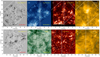 |
Fig. 1. Full FOV of the observations corresponding to data sets 1 (top row) and 2 (bottom row). Top row, panel a: Hα red wing image observed with CRISP at a Doppler offset of +40 km s−1, panel b: corresponding CHROMIS Ca II K line core image, and panels c and d: co-spatial Si IV 1400 Å SJI from IRIS and the 171 Å image from AIA, respectively. Bottom row, panel a: Hα red wing image observed at a Doppler offset of +36 km s−1 acquired with CRISP, and panels b–d: corresponding co-spatial cutouts from AIA 304 Å, the IRIS Si IV 1400 Å SJI, and AIA 171 Å, respectively. The dashed vertical lines correspond to the spatial extent of the IRIS rasters in the two data sets, and the direction to solar north is pointing upward. The white and cyan boxes in the top and bottom rows represent the area of the Ca II K core and the Hα red wing images, respectively. Animations corresponding to these figures are available online. |
Data set 2 focused on a quiet Sun region at the disk center located around solar (X, Y) = (−1″, 1″) shown in the bottom row of Fig. 1. The duration of this data was 59 min starting from 08:23 UT and lasting until 09:22 UT. CRISP recorded imaging spectroscopic data in Hα and Ca II 8542 Å, in addition to spectropolarimetric data in Fe I 6173 Å. The Hα spectral line was sampled at 31 wavelength positions between ±1.5 Å, in steps of 100 mÅ, Ca II 8542 Å was sampled at 9 wavelength positions between ±0.8 Å, in steps of 200 mÅ, and Fe I 6173 Å was sampled at 14 wavelength positions between −0.32 Å and +0.68 Å with respect to the line cores. The temporal cadence of the time series was 23.6 s with a spatial sampling of  . High spatial resolution down to the diffraction limit of the telescope (given by λ/D =
  at 6563 Å) was achieved through high-quality seeing conditions, the SST adaptive optics system (Scharmer et al. 2019) and the Multi-Object Multi-Frame Blind Deconvolution (MOMFBD) technique described in van Noort et al. (2005). We used the SSTRED reduction pipeline (de la Cruz Rodríguez et al. 2015; Löfdahl et al. 2021) to facilitate further reduction of the data, while including the spectral consistency technique outlined in Henriques (2012). Furthermore, intra-CRISP alignment between Hα and Ca II 8542 Å was achieved by cross-correlating the corresponding photospheric wideband images, followed by a de-stretching procedure to compensate the warping due to seeing effects. In this study we only focus on the spicular downflows observed in the red wings of Hα.
IRIS ran in a large-dense four-step raster mode (OBS-ID 3633109417), co-observing the same FOV as SST. The raster cadence was 36 s (with a step cadence of 9 s and an exposure time of 8 s per slit position) and the FOV covered by the spectrograph slit was  in the solar X and Y direction. Moreover, it also recorded SJIs in the 2796 Å channel (that is dominated by the inner wings and core of the Mg II k spectral line), and Si IV 1400 Å channel with a cadence of 18 s covering a FOV of 120″ × 120″. The high exposure time (in comparison to data set 1) of this data set enabled better visibility of the different features in the Si IV channel.
The IRIS data were co-aligned to SST by cross-correlating Ca II 8542 Å data (integrated over the entire wavelength dimension) with the SJI recorded in the 2796 Å channel (expanded to the CRISP pixel scale of  ). The summation over the wavelength resulted in images that bore a close resemblance to the features observed in the 2796 Å channel thereby enabling better correlation. The resulting IRIS data were finally cropped so as to have a common FOV of 70″ × 70″ with SST. Panels a, and c in the bottom row of Fig. 1 show the co-aligned SST CRISP image observed in the red wing (+36 km s−1) of Hα and the corresponding Si IV 1400 Å SJI, respectively. The coordinated data sets (both 1 and 2) will be made publicly available in the future as a part of the SST–IRIS database (Rouppe van der Voort et al. 2020).
Observations from the Solar Dynamics Observatory. For both data set 1 and data set 2, we downloaded corresponding SDO image cutout sequences. These sequences were cross-aligned – all AIA channels to Helioseismic Magnetic Imager (HMI) continuum – and then the HMI continuum images were finally co-aligned to the Ca II K and Ca II 8542 Å wideband channels for data set 1 and 2, respectively. We used an Interactive Data Language (IDL) based automated aligning procedure developed by Rob Rutten for this purpose, which is publicly available at his website1. For a precise cross-alignment among the SDO channels, the procedure collects and downloads two sets of SDO cutouts – one at full cadence focusing on the smaller target area (SST wideband) and the other large ones (700″ × 700″) around disk center at a lower cadence. The latter set is used to find offsets between the different channels by cross-correlation of smaller subfields covering roughly 30″ × 30″, and by applying the height-of-formation differences in an iterative fashion. Since both the data sets are close to the disk center, the projection effects are likely lower, which suggests that the accuracy of cross-alignment could be on the order of an AIA pixel ( ) or possibly less, depending on the overall magnetic topology. We refer the reader to Rutten (2020) for more details. Each co-aligned SDO data set comprises eleven (nine AIA and two HMI) image cutout sequences that are resampled from their original pixel scale (
 ) to the CHROMIS and CRISP pixel scale of
  and
and  respectively for the two data sets and are chosen such that they are as close as possible in time (through nearest-neighbor selection) with respect to one another. Sample co-aligned SDO AIA images are shown in panel d (top row) and panels b and d (bottom row) of Fig. 1. For the purpose of the analysis presented in this paper, we use only the EUV AIA 304 Å, 171 Å, and 131 Å sequences.
2.2. Numerical simulation
For the purpose of comparing the observed properties of the downflowing RREs, we use 2.5–dimensional (2.5D) radiative MHD numerical simulation of spicules from Martínez-Sykora et al. (2017a,b). This simulation was performed using the state-of-the-art Bifrost code (Gudiksen et al. 2011), including ambipolar diffusion2 to model spicule generation. Contrary to older Bifrost simulations, high-speed (∼50−100 km s−1), thin, needle, spicule-like features were produced naturally in this case and they occurred ubiquitously throughout the simulation domain. The importance of ambipolar diffusion along with large-scale magnetic fields (that is, magnetic loops with length ∼50 Mm) and high spatial resolution were found to be crucial for the simulated spicular ubiquity. Furthermore, this model also successfully reproduced various observed properties of type-II spicules such as strongly collimated flows (∼100 km s−1) that reach up to 10 Mm in height within a lifetime of up to ∼10 min. Most of the spicular activity is concentrated around network and plage regions, which is also compatible with observations.
The simulation domain spans from 2.5 Mm below the visible photosphere up to about 40 Mm into the corona with resolution varying from 12 km to 60 km in the vertical direction. The horizontal domain spans 96 Mm with a uniform resolution of ∼12 km. Figure 2 shows an overview of the simulation snapshot with the top row showing a 2D map of temperature and the bottom row showing the corresponding vertical velocity. The type-II spicules appear as cooler chromospheric intrusions into the hot corona. For the sake of visualization, the vertical domain has been limited to only 12 Mm. The complex physical processes that lead to the generation of spicules, along with other details of the simulation setup has been described extensively in Martínez-Sykora et al. (2017a,b, 2018).
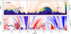 |
Fig. 2. Overview of the MHD simulation snapshot from Martínez-Sykora et al. (2017b) showing a 2D slice of temperature (top row) and signed vertical velocity vz (bottom row) at t = 190 s from the start. The spicules appear as cool finger-like intrusions in the hot corona, and the ones that are further analyzed are numbered 1 and 2. Velocities away from the observer are indicated in red (positive) and toward the observer in blue (negative). The contour indicates the location where the temperature equals 30 kK. The region to left of the dashed vertical line in the bottom row indicates the region of interest that is further studied in Sect. 5.3. An animation of this figure is available online. |
3. Method of analysis
3.1. Identification of the downflowing spicular events
The downflowing RREs, like RREs, show significant absorption asymmetries in the red wing of the Hα spectral line. This formed the basis of an automated detection algorithm based on the k-means clustering technique, which enabled the detection of tens of thousands of spicular events, including the downflowing RREs, RBEs, and RREs in data set 1. The details of the algorithm along with the advanced morphological processing techniques have been described in Bose et al. (2019a), and more recently in Bose et al. (2021). In this paper, we simply use those detections and overlay them on the co-aligned IRIS and SDO data sets to study their responses in the transition region and the solar corona.
For data set 2, we relied on a detection method that is based on the morphology of the events observed in the far red wing (+36 km s−1) of the Hα spectral line, as shown in the bottom row of Fig. 1. The events were selected by constructing Hα Doppler maps (blue – red wing image subtraction at ±36 km s−1) where the RBEs show up as dark streaks, while the RREs (downflowing RREs) show up as bright ones. Simple thresholding based on intensity of the resulting Doppler maps, led to the extraction of spicular features in the red wing of Hα. This approach has been used in the past to detect RBEs and RREs, and we refer to Rouppe van der Voort et al. (2009, 2015) and Henriques et al. (2016) for more details. We relied on a simpler detection method for data set 2 because the major goal was to simply extract the location of the downflowing RREs so that we could investigate their responses in hotter passbands on an event-by-event basis, rather than focusing on their detailed statistical characterization. Moreover, the idea was also to highlight that the downflowing RREs are equally ubiquitous in regions with different magnetic field environments. These detections were further confirmed by extensive visualization using CRISPEX (Vissers & Rouppe van der Voort 2012), a widget-based analysis tool written in IDL. The animations associated with Fig. 1 clearly convey that both the data sets are replete with downflowing RREs (in the chromosphere), whose apparent motion is directed toward the strong network regions, opposite to what we typically observe in RBEs and RREs (see Rouppe van der Voort et al. 2009; De Pontieu et al. 2012; Sekse et al. 2012, 2013; Kuridze et al. 2015, and references therein).
In both data sets 1 and 2, the detected events were then simply overlaid on the corresponding co-aligned IRIS and SDO data sets to study their responses in the transition region and the solar corona. To aid visibility, we subtracted an average over the whole time series from each AIA image on a per-channel basis. This is done separately for the 131 Å, 171 Å, and 304 Å channels, which ensured the removal of the effect of long-lived brighter structures (e.g., loops) along the enormous line-of-sight (LOS) superposition in an optically thin plasma. Finally, the events, now observed across the different wavelengths (from SST, IRIS, and SDO), were again analyzed and visualized using CRISPEX. The evolution of the downflowing RREs was highlighted by constructing space-time (X − t) maps for each event that are generated by computing the average over the highlighted regions for each time step.
3.2. Optically thick and thin radiative transfer
We used the RH1.5D3 (Pereira & Uitenbroek 2015) radiative transfer code for optically thick radiative transfer calculations. RH1.5D is a massively parallelized version of the former RH radiative transfer code by Uitenbroek (2001). It is capable of performing multi-atom, multilevel nonlocal thermodynamic equilibrium (non-LTE) radiative transfer computations under both partial and complete frequency redistribution (PRD and CRD). Moreover, it can also synthesize full Stokes parameters while including Zeeman splitting effects. This code can compute synthetic spectra from 3D, 2D, or 1D model atmospheres on a column-by-column (1.5D) basis. It also scales well to at least thousands of CPU cores and can be easily run over multiple nodes in a supercomputing cluster.
We used the RH1.5D code to generate synthetic Ca II K and Mg II k spectra from the 2.5D numerical simulation described in Sect. 2.2. The goal of this analysis is to compare the spectral properties of type-II spicules from the simulation with available observations from IRIS and SST. Such an investigation leads to a detailed understanding of spectral line formation in stellar atmospheres. We used a five-bound-level plus continuum model of the Ca II ion, as used by Bjørgen et al. (2018) and a ten-level plus continuum model of the Mg II atom used by, e.g., Leenaarts et al. (2013) and Bose et al. (2019b), under PRD and 1.5D geometry. The fast angle hybrid approximation scheme was used for PRD calculations as described in Leenaarts et al. (2012). The initial level populations were estimated by assuming a zero mean radiation field and solving the statistical equilibrium equations. This approach works better than starting with LTE populations, for instance, since atoms with strong lines have level populations that are significantly different from LTE (Pereira & Uitenbroek 2015). The effects of PRD are important in the region where the K2/k2 emission peaks are formed since radiative damping is much larger than collisional damping (Sukhorukov & Leenaarts 2017; Bjørgen et al. 2018). Furthermore, these emission peaks along with the wings of resonance lines under consideration, such as Ca II K and Mg II k, are formed deeper in the solar atmosphere in comparison to the line core, where the effect of horizontal radiative transfer is small, thereby justifying the 1.5D treatment. The computed specific intensity is further spectrally and spatially smeared with the SST and IRIS instrumental point spread functions to compare with the observations.
The analysis of synthetic intensity corresponding to the Si IV 1393 Å spectral line is computed assuming optically thin approximation under ionization equilibrium of Si IV, in a way similar to Martínez-Sykora et al. (2016), for example. We use the CHIANTI database (Dere et al. 2009) to synthesize the plasma emission with the ionization balance available in the CHIANTI distribution and using the Si IV abundance from Asplund et al. (2009) – more specifically, 7.52 in the customary astronomical scale, where 12 corresponds to hydrogen. The resulting emission spectra was convolved with the IRIS spectral transmission function before comparing with the observations.
4. Results
4.1. Transition region and coronal response to downflowing RREs
Figure 3 shows three examples of downflowing RREs along with their signatures in the transition region and coronal passbands. The vertical dashed lines in the figures show the region that is used to construct the X − t maps to study their evolution. The top row of the figure and its associated animation shows the evolution of a typical downflowing RRE observed in data set 1 in the far red wing (+40 km s−1) of Hα and its corresponding signature in the AIA 304 Å, 131 Å, and 171 Å passbands. These passbands are dominated by spectral lines from He II, Fe VIII, and Fe IX ions that are formed primarily around 0.1, 0.4 and 0.8 MK, respectively (Lemen et al. 2012). A detailed analysis of the synthetic emission of various AIA passbands from 3D MHD simulations by Martínez-Sykora et al. (2011) indicated that the above mentioned channels were least influenced by nondominant ionic species, thereby suggesting that the major contribution to the emission mostly comes from the dominant ions specified earlier. The apparent inward motion (i.e., toward the bright points) is clearly revealed from the X − t maps and also from the animation. While the HαX − t map shows signatures of the downflow starting around t = 170 s, a close look at the corresponding maps in the hotter passbands of AIA, especially the 171 Å channel, show that the feature is already present close to t = 0 s. The 304 and 131 Å channels also show faint signatures toward the beginning of the evolution. The animation associated with the Hα red wing image also shows a small horizontal displacement of the bright network element close to the footpoint of the downflowing RRE from ∼(X, Y) = ( ) to ∼(X, Y) = (
 ) during its evolution. This transverse displacement can have a LOS component causing the apparent downward motion; however, given the fact that the displacement (by
  ) is small and strictly in the horizontal direction with a velocity of roughly 2 km s−1, it is unlikely to affect the vertically downward apparent motion shown by the downflowing RRE, which has a significantly higher velocity of roughly 30 km s−1 (deduced from the HαX − t map). Moreover, the location of the coronal plasma with respect to the chromospheric downflowing RRE seems to vary substantially with temperature, with a clear spatial offset of the hottest emission above the cooler chromospheric plasma. Since the accuracy of the cross-alignment between the AIA channels is found to be better than the AIA pixel scale, it is likely that this offset (of roughly 1″) is attributable to the downflowing RRE. This suggests the possibility that the downflowing RREs have a multi-thermal nature and can be heated to at least lower coronal temperatures roughly at 0.8 MK.
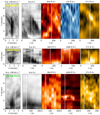 |
Fig. 3. Space-time (X − t) diagrams for three representative downflowing RREs, on 25 May 2017 (top row) and 19 September 2020 (middle and bottom rows), showing their multi-thermal nature across multiple wavelength channels. The dashed vertical lines in the Hα red wing images indicate the region along which the X − t maps have been extracted in the coordinated SST, IRIS, and SDO data sets. The different panels in each row corresponds to the X − t maps in the different wavelength channels as indicated at the top. The solid white vertical lines in the X − t maps correspond to the time step at which these maps have been shown. Animations of this figure are available online. |
The lack of signature in the first half of the HαX − t map could be primarily because the downflowing RREs, like traditional RREs and RBEs, have a wide range of Doppler shifts associated with them (Pereira et al. 2016; Bose et al. 2021). Therefore, it is possible that observations in the wing positions, closer to the line core of Hα spectral line, can overcome this gap to some extent. This can be further supported by taking a closer look at the Hα spectral-time evolution diagrams of some additional examples from data set 1 (shown in Figs. 4–6 and described further in Sect. 4.2), which provides an impression that the downflowing RREs have roughly zero Doppler shifts during their initial phases, which increases gradually with time.
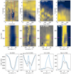 |
Fig. 4. Representative example of a downflowing RRE observed in the SST, IRIS, and SDO data sets acquired on 25 May 2017 and its spectral signature across the different chromospheric and transition region spectral lines. Top row (left to right): Hα red wing image showing the downflowing RRE at +40 km s−1, X − t maps (extracted from the region bounded by the two dashed red lines) corresponding to the Hα red wing at +40 km s−1, the IRIS Si IV 1400 Å SJI, and the AIA 171 Å channels. Middle row (from left to right): λt diagrams in Hα, Ca II K, Si IV 1393 Å, and Mg II k, respectively, corresponding to the spatial location marked with a white cross in the Hα red wing image. Bottom row: corresponding spectral profiles for the different wavelengths at the instant of maximum redward excursion (magenta marker) indicated in the λt diagrams. The dashed spectral profiles correspond to the spatial and temporal average over the whole time series in each case. The observed intensity is shown in arbitrary units. |
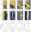 |
Fig. 5. Second representative example of a downflowing RRE observed on 25 May 2017 in the same format as Fig. 4. |
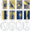 |
Fig. 6. Third representative example of a downflowing RRE observed on 25 May 2017 in the same format as Fig. 4. |
The middle and the bottom rows of Fig. 3 show two additional examples of multi-thermal downflowing RREs from data set 2 in the same format described above. Like before, here also we find emission signatures in the transition region and coronal passbands corresponding to the chromospheric downflows. The IRIS Si IV 1400 Å channel, sampling roughly 0.08 MK, is shown in these examples instead of the AIA 131 Å passband, since the signatures in the latter is not as prominent. The X − t maps appear to be coarser in comparison to the earlier example because the temporal cadence of data set 2 (23.6 s) is lower than data set 1, and the downflows last for a shorter period of time. The animation associated with this figure provides a clearer impression of the apparent motions associated with the two events. Unlike the example in the top row, here we see a co-temporal downflow in all channels including the Hα red wing. This could be due to the image being observed at a line position that is closer to the Hα core. Based on the Si IV 1400 Å X − t maps, we also find that the plasma associated with the downflowing RREs is at least sometimes heated to transition temperatures throughout its evolution. It is also to be noted that, unlike the middle row, the Si IV channel corresponding to the downflowing RRE in the bottom row does not show significant emission toward the later stages of evolution starting roughly around 150 s. The hotter 171 Å channel also shows strong emission throughout the evolution of the downflowing RREs except in the middle row where the signal starts to appear only toward the later half. Similarly, the 304 Å passband shows a gradual enhancement in emission as the evolution progresses with a substantial emission around t = 100 s (middle row). The spatial offset between the hotter coronal and cooler chromospheric plasma is even more prominent in the bottom row indicating that the hotter material lies on top of the cooler plasma. The scenario described here suggests that downflows are not completely heated to transition region (or even coronal temperatures) and are likely multi-threaded with cold and hot threads. We also note that the downflowing RRE shown in the middle row has a smaller spatial extent in comparison to the other two rows, roughly covering 6−7 AIA pixels in the Y direction. However, the apparent motion in the AIA channels show strong emission that is well correlated with the corresponding signature in the HαX − t map. This suggests that some downflows can also have a small blob-like appearance, contrary to elliptical shapes that is commonly observed in spicules.
In both examples, the X − t maps suggest that the apparent velocity of the chromospheric, transition region and coronal plasma is probably very similar, with velocities in the range between 25−40 km s−1, and they move (inward) toward the bright network regions. It is to be noted that we did not find any associated signature in the blue wings of Hα preceding the downflowing RREs. This has already been shown to be the case for a few downflowing RREs by Bose et al. (2021), and will be discussed in detail in the following section. Moreover, we also suggest an alternate mechanism from the numerical simulations in Sect. 5.3 that could likely explain the appearance of such downflows without preceding blueward excursions.
4.2. Spectral signatures
The spectral signatures of the downflowing RREs in the solar chromosphere (mainly in Hα) were already discussed in Bose et al. (2021). In this paper, we aim to show their signatures observed in the lines formed in the upper chromosphere and transition region. The spatial coverage of the IRIS rasters is limited as compared to the SST FOV. Therefore, the number of downflowing RREs overlapping on the IRIS raster at a given time is limited. Moreover, despite being quasi-simultaneous, there could be residual temporal offsets between the SST and IRIS rasters on the order of 3−4 s, which can cause a further limitation. The examples described in Sect. 4.1 do not overlap the IRIS rasters and therefore have no spectral information. In this section we highlight a few examples from data set 1 where the downflowing spicular events overlapped co-temporally and co-spatially in all three (SST, IRIS–SJI+raster, and SDO) instruments.
Figure 4 shows an example of a downflowing RRE with the temporal evolution indicated with the help of X − t maps in the different passbands in the top row, while the middle row shows the spectral evolution in the form of λt (spectral–time diagrams) in Hα, Ca II K, Si IV, and Mg II k, respectively from left to right. The dashed red lines in the Hα red wing image at +40 km s−1 indicate the region selected for generating the X − t maps for the different passbands, which clearly show the apparent inward motion in all the channels. This suggests enhancement to temperatures as high as 0.8 MK during the downflow based on the emission pattern in 171 Å. Furthermore, a closer look at the X − t diagrams reveal that Hα shows fainter signal in the period between 0 and 100 s whereas the Si IV 1400 Å and 171 Å channel shows significant emission. This could hint that during the initial stages, the downflow is too hot to be detected clearly in the Hα red wing images, which was perhaps also the case in the example shown in the top row of Fig. 3. Such behavior is compatible with a multi-thermal nature in the downflowing RREs.
The λt diagrams reveal the temporal evolution of the spectral profiles at a given spatial location of the downflowing RRE. The excursion toward the redward side of the Hα line center is nearly co-temporal with the excursions of the central absorption K3 (k3) feature in the Ca II K (Mg II k) diagrams, and a strong redward emission in the Si IV 1393 diagram. We see a typical development of a highly asymmetric line profile peaking out at 20−40 km s−1 redward of the nominal line center in all the cases. This is further illustrated in the bottom row of Fig. 4, where spectral profiles corresponding to the time of maximum redward excursion in Hα are shown. The Ca II K and Mg II k spectral lines show a redshift in the central absorption K3 (k3) feature with respect to the average profiles (constructed from temporal and spatial average over the entire FOV for Ca II K and over all the slit positions for Mg II k), which causes the K2r and k2r emission peaks to disappear completely. Furthermore, an enhancement in the K2v and k2v peaks is also seen that makes it well aligned with the observations by Rouppe van der Voort et al. (2015) and optically thick line formation mechanism in spicules described in Bose et al. (2019a).
The Si IV 1393 Å spectra are generally noisier at this exposure time (2 s). Nevertheless, a comparison of the λt diagram with other panels show similar temporal behavior with redward asymmetric excursions that are in tandem with their pure chromospheric counterparts Hα, Ca II K and Mg II k. Preliminary analysis based on single Gaussian fits to the far-UV spectra indicates a Doppler shift on the order of 15−20 km s−1 for the downflowing RRE, which is slightly higher than the values reported by Rouppe van der Voort et al. (2015) for traditional RREs.
Figures 5 and 6 show two additional examples of downflowing RREs in the same format as Fig. 4. Like the earlier cases, we clearly see the multi-thermal behavior of the downflowing RREs based on their near co-temporal visibility in the 1400 Å and 171 Å along with Hα red wing X − t maps. A noticeable distinction among the three examples is that the emission pattern of 171 Å shown in Fig. 4, appears to occur over a larger spatial region and is colocated with the appearance of the dark spicular region in Hα in comparison to the other cases, where we clearly see the emission confined to narrower bright streaks. This difference is also apparent to some extent in the examples shown in Fig. 3. Furthermore, the 171 Å emission seems to weaken toward the later part of the evolution of the downflowing RREs (in Figs. 5 and 6), though the inward apparent progression remains evident. Contrary to Figs. 4 and 5, the emission pattern in the 1400 Å X − t map observed in Fig. 6, lasts for a shorter period of time (∼30 s) around t = 100 s. The inward apparent motion (downflow) is also not very prominent like in the other wavelength channels. This could be mainly attributed to either the low exposure time of the acquired SJIs or the downflowing RRE not being hot enough throughout its evolution or a combination of the two. The evolution in the adjacent 171 Å map seems to support the scenario that the downflowing RRE indeed cools down after t = 100 s (or so), since the emission is significantly reduced. Also, with the exception of Fig. 4, at any given time the emission corresponding to 171 Å appears to have a slight offset in the Y direction in comparison to the cooler chromospheric component. This seems to also be the case when the transition region brightenings are compared with Hα. This is similar to the examples shown in the top and bottom rows of Fig. 3. Therefore, it suggests the possibility of a scenario where the hot plasma (∼0.1−0.8 MK) lies above the cooler chromospheric component at ∼0.01 MK, once again revealing the multi-thermal nature of downflowing RREs, similar to RBEs and RREs (De Pontieu et al. 2011; Pereira et al. 2014; Skogsrud et al. 2014).
The λt diagrams and the corresponding spectral profiles at the time of maximum excursion of the downflowing RREs show similar properties to what has been described earlier in Fig. 4. In fact, the two downflowing RREs shown in Figs. 5 and 6 show stronger absorption asymmetries toward the redward side of the line center both in Hα and Ca II K. Even the emission corresponding to Si IV 1393 Å appears to have a stronger excursion when compared against Fig. 4. A closer look at the Ca II K spectral line shown in the bottom row of Fig. 6 reveals significant enhancement in its specific intensity (including the line wings) in comparison to the Ca II K spectral profiles shown in the other examples. This is attributed to the bright network regions in the background of the spicule, which is clearly visible in the Hα red wing image. Nevertheless, the asymmetry in the line profile with a shift of the K3 line core toward the redward side of the line center, along with the enhancement in the K2v peaks is apparent in all the three cases. The redshift of the k3 core in the Mg II k spectral profile shown in the bottom row of Fig. 5, does not completely eliminate or suppress the k2r peak as evident in the other examples. However, like Ca II K, the asymmetry is clear enough with the k2v peak being enhanced in comparison to the k2r indicating the presence of strong velocity gradients in spicules that remove the upper-layer opacities at the k2v wavelengths.
In the examples described in this section, the λt diagrams (for all wavelengths) do not show signs of preceding blueshift that are typical for type-I spicules. This is suggestive of an alternate mechanism (based on loops) that could also be responsible for the observed downflowing RREs. This is discussed further in Sect. 5.3. We also find that the Doppler shifts associated with the downflowing RREs (25−50 km s−1) are compatible with their apparent velocities of the corresponding transition region and with coronal brightenings. The compatibility of the apparent motion and the observed Doppler shifts indicates that the downflows studied here are basically a result of real plasma (mass) flows that are different than the high-speed (100−300 km s−1) apparent motions often associated with transition region network jets (Tian et al. 2014). Such high speeds in the network jets are possibly caused by rapidly propagating heating fronts rather than mass flows (De Pontieu et al. 2017a).
The properties of the Hα, Ca II K, and Mg II k line profiles for the downflowing RREs described in this section are well aligned with the spectral characteristics of RREs (downflowing RREs) reported by Bose et al. (2019a). Characterizing millions of RBE and RRE spectral profiles belonging to Ca II K, Hα, and Mg II k with the statistical k-means clustering technique, they found that opacity shifts with strong gradients in the LOS velocity are dominant among spicules. Interestingly, they also reported that the RRE or downflowing RRE-like Ca II K and Mg II k spectral profiles are, on average, broader than the RBE-like profiles, and have significantly enhanced K2v (k2v) peaks when compared both against the average profiles (over the whole FOV and time series) and RBE-like profiles (refer to Fig. 3 in Bose et al. 2019a). This hinted a possibility of other mechanisms, likely heating-based, in the RREs and downflowing RREs. The chromospheric spectral characteristics shown in this study clearly correlate with the earlier observations and point toward a possibility where the downflowing RREs do undergo heating during their evolution. In the following section, we investigate this scenario with the help of an advanced MHD simulation.
4.3. Comparing synthetic observables from MHD simulation
4.3.1. Radiative transfer diagnostics
A valid comparison between any numerical simulation and observation is only possible by accounting for the radiation transport of photons through the simulated stellar atmosphere, since the only source of information available from observations is the intensity at specific wavelengths of interest. In this section, we show synthetic spectra for a typical spicule (spicule 1 in Fig. 2) for the lines formed in chromosphere and transition region. The details of the simulation have been described in Sect. 2.2.
We tracked the complete evolution of spicule 1 but we restrict ourselves to the two phases shown in Fig. 7 for the sake of brevity. Phase 1 in the top row is the rising or upflowing phase of the spicule shown at roughly 140 s after the start of the simulation, while phase 2 (bottom row) is the downflowing phase, which occurs about 230 s later. The animation associated with Fig. 2 shows that the upflowing phase is characterized by strong initial velocities on the order of 50−70 km s−1 toward the observer (the direction is relative to the observer looking vertically downward), while the downflowing phase has strong velocities of at least 30 km s−1 away from the observer. These velocities are similar to what has been observed in the on-disk manifestations of type-II spicules such as RBEs, and RREs and downflowing RREs (Rouppe van der Voort et al. 2009; Sekse et al. 2012, 2013; Henriques et al. 2016; Bose et al. 2021). In the simulation, we refer to phase 2 or the returning phase of spicule 1 as a downflowing RRE.
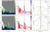 |
Fig. 7. Synthetic observables of the chromospheric and transition region spectral lines obtained from the numerical simulation. Top row (left to right): a cutout of the 2D temperature map, the signed vertical velocity around spicule 1, and the Ca II K, Mg II k, and Si IV 1393 Å synthetic spectra corresponding to the upflowing phase of the spicule at t = 140 s. Bottom row: corresponding temperature, vertical velocity, and synthetic spectra for the downflowing phase of the spicule at t = 370 s in the same format as the top row. Temperatures beyond 30 kK have been masked in the 2D temperature maps and are indicated with a black contour in the vertical velocity maps. The dashed vertical blue line corresponds to the LOS of the observer along which optically thick (thin) radiative transfer is performed. |
In the last column of Fig. 7 synthetic Ca II K, Mg II k and Si IV 1393 Å spectral profiles for both the upflowing and downflowing phases are shown. Radiative transfer computations were performed along the direction of the dashed blue vertical marker with the observer looking down. The upflowing phase in the optically thick lines show distinct shifts in the K3 (k3) core toward the blueward side of the respective line centers that suppresses the K2v (k2v) peaks, while causing an enhancement in the opposite emission peaks. The trend is quite pronounced for the Ca II K spectral line but to a lesser extent in Mg II k. This is because the two spectral lines are sensitive to slightly different atmospheric regimes, which affects their line formation mechanism. This will be discussed further in Sect. 4.3.3. The hotter Si IV profile shows a blueward shift of its peak that is well correlated with K3 and k3 line cores.
The Ca II K and Mg II k profiles corresponding to the downflowing stage at the same spatial location show significant enhancement in their radiation temperatures in comparison to the upflow. Furthermore, the shift of the K3 (k3) core toward the redward side of the respective line centers is so strong that it completely makes the K2r (k2r) peak disappear. The local emission peak corresponding to the orange Ca II K profile at Δλ ≈ 15 km s−1 can be mistakenly interpreted to be the reduced K2r (and the observed “valley” immediately blueward of this peak to be K3), but a detailed analysis based on contribution function suggests that it is not the case. We refer the reader to Sect. 4.3.3 for a more in-depth discussion. For the Si IV emission line, not only is the peak strongly redshifted, the line also appears to be broader compared to its upflowing counterpart. The radiation temperature, corresponding to the peak emission, is also slightly higher than the upflowing phase but overall the Si IV line has weaker emission in comparison with the optically thick lines. These observations are well correlated with the spectral signatures of the downflowing RREs described in Sect. 4.2 and Figs. 2 and 3 of Bose et al. (2019a). Moreover, a close comparison of the temperature maps shown in the first column of Fig. 7 reveal a marked increase in temperature toward the tip of the spicule during the downflowing phase. This increase in temperature could indicate signs of heating during the downflowing phase of spicules. This forms the basis of the results presented in Sect. 4.3.2.
4.3.2. Heating in the downflowing RREs
The analysis presented in Fig. 7 indicates that the downflowing phase of spicule 1 is marked with an enhancement in both the gas (plasma) temperature and radiation temperature of spectral profiles. In this section, we investigate the cause of this enhancement by exploiting the physical parameters obtained from the numerical simulation.
Figure 8 shows the complete thermodynamic evolution of the two spicules of interest. The spicules have different inclination with respect to the LOS of the observer and each panel displays two columns, where the left column shows the thermodynamic quantities being investigated (i.e., temperature, energy, and the summation over various heating parameters normalized by the number density) and their corresponding time evolution are indicated with X − t maps shown on the right. In both examples, we masked out regions from the FOV where the temperature exceeded 30 kK because both Mg II and Ca II ionizes well below this temperature. We consider heating in the spicules due to Joule dissipation, ambipolar diffusion, viscosity, thermal conduction, and radiative terms that can be directly obtained from the Bifrost code. Ambipolar diffusion refers to the diffusion between charged species and neutral particles that plays a key role in the solar atmosphere where the plasma is partially ionized. The radiative terms refer to optically thin losses, radiative losses by neutral hydrogen, singly ionized calcium, and magnesium, and heating by incident UV radiation from the solar corona (Carlsson & Leenaarts 2012).
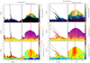 |
Fig. 8. Spatio-temporal evolution of the different thermodynamic parameters obtained from the MHD simulation. The left column of panel a shows the 2D maps of temperature, internal energy, and the sum over heating parameters (as described in the text) per particle (ρ being the plasma density), and the right column indicates the space-time maps corresponding to each of the physical quantities for spicule 1. The two columns of panel b shows the spatio-temporal evolution corresponding to the same physical quantities for spicule 2, in the same format as panel a. The dashed lines in the left column of the two panels show the bounding regions that are considered for extracting the X − t maps (shown in the respective right columns), and the vertical red line in the X − t maps corresponds to the time steps at which these maps have been shown. Animations of this figure are available online. |
The two panels and their associated animations show the complete evolution of the two spicules. Upon closer investigation, we see that the temperature starts to show enhancement right at the time when the spicules reach their maximum extent (or completing the upflowing phase), and initiate the downflow. The enhancement is more significant for spicule 2 with temperatures reaching as high as 20 kK during the maximum excursion phase. Overall, in both cases, we find that the temperature increases from 7 to 9 kK during the start of the upflowing phase and continues to increase until it reaches the peak of the parabolic trajectory, where it reaches as high as 18−20 kK. This is found to be in agreement with the analysis by Martínez-Sykora et al. (2017b, 2018) and De Pontieu et al. (2017a). The energy maps follow the temperature very closely showing similar parabolic trajectories, but unlike temperature, they do not show any substantial difference between the two phases. This is, in part, related to the fact that the density of the spicules decreases as they evolve. We refer the reader to Sect. 5.2 for further discussions.
The sum over the heating terms normalized by number density, shown in the last row of the two panels in Fig. 8, display a compelling visual correlation with the corresponding temperature X − t maps in the top row. The correlation is quite striking for spicule 1 where we see that the heating actually increases right around the time when the temperature starts to show enhancement (at about t = 250 s), and it continues to remain significantly heated covering almost the entire downflowing phase of the spicule. The enhancement in heating is also quite significant for spicule 2, and it also occurs around the same time as the temperature gets enhanced (at about t = 250 s). However, unlike spicule 1, the heating tends to get weaker toward the end of the downflowing phase. Nonetheless, both spicules clearly show heating toward the end of the upflowing phase and beginning of the downflowing phase, which correlates well with the behavior observed in the temperature maps. Moreover, the temporal duration of enhanced heating is similar in both cases lasting roughly 200 s.
The results from the MHD simulation presented in this section provide a clear indication that the downflowing (downflowing RRE) phase of the spicules is indeed hotter in comparison to the upflow (RBE) as we inferred from the observed and synthetic spectral profiles.
4.3.3. Contribution function analysis for optically thick lines
In Sect. 4.3.1 we saw that the Doppler shift of K3 core in the synthetic Ca II K spectral line enhances or suppresses the respective K2 peaks, but the effect may not be similar in Mg II k. For example, the synthetic Ca II K spectra for the upflowing phase shows a significant asymmetry in the K2 peaks in Fig. 7, whereas the effect (though evident) is far less pronounced in the corresponding Mg II k spectra. Moreover, the downflowing phase shows a complete suppression of the Mg II k2r peak but we find a residual K2r in Ca II spectra. A similar remark can also be made from the observed downflowing RREs described in Sect. 4.2. These differences can be attributed to the fact that different spectral lines are sensitive to different regions in the solar atmosphere. We aim to understand the Ca II K and Mg II k spectral line formation observed in spicules based on contribution function analysis.
We used the method described in Carlsson & Stein (1997) to compute the contribution functions for Ca II K and Mg II k spectral lines formed during the upflowing and downflowing phases of spicules at the time steps and along the dashed vertical marker in Fig. 7. The contribution function CI was decomposed to the emergent intensity by
into three parts – χ/τ, S, and τ exp(−τ) – which are shown in panels a–d of Fig. 9 in the form a classical 4-panel diagram. The dependence on frequency (or wavelength) is shown along the X-axis, and the Y-axis shows the variation in the components along the geometric height scale z. On each panel we plot the vertical velocity as a function of geometric height (yellow solid) and optical depth unity as a function of frequency given by τν = 1 (white solid).
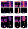 |
Fig. 9. Intensity formation breakdown figure for the Ca II K and Mg II k spectral lines corresponding to spicule 1 from the model atmospheres at the location indicated by the vertical marker in Fig. 7. Panel a: formation of the Ca II K spectral line at t = 140 s (upflowing phase). Panel b: formation of the Ca II K spectral line at t = 370 s (downflowing phase) with a strong asymmetry toward the redward side of the line center. Panel c: formation of the Mg II k line for the upflowing phase. Panel d: formation of a single peaked Mg II k spectral line for the downflowing phase. Each sub-panel shows (dark corresponds to low values and orange corresponds to high values) the quantity indicated at the top left corner as a function of geometric height z and frequency from the line center in km s−1. The τν = 1 curve (white) and vertical velocity (yellow, positive is downflow) are overplotted in each sub-panel. The solid gray line (indicating zero Doppler shift) is shown in the first sub-panels for reference. In addition, the first sub-panels show the ionization fraction (dotted cyan line) of Ca II (panels a and b) and Mg II (panels c and d) as a function of z. The upper right sub-panels also contain the plasma temperature (dashed green) as a function of z in logarithmic scale, specified along the top. The lower right panel also shows the specific intensity profiles (cyan) as radiation temperature with units specified on the right-hand side. |
The first component shows the ratio between the total opacity χ and optical depth τ. This is important when there are multiple emitting species (large χ) at small optical depths. Moreover, this factor is also responsible for the asymmetry of spectral lines that is typical for atmospheres where there is a large velocity gradient (as is the case for spicules). In addition, we also show the ionization fraction of Ca II to Ca III as a function of height (dotted cyan).
The total (line plus continuum) source function (S) forms the second component that is strongly dependent on frequency for lines that are affected by PRD (such as Ca II K and Mg II k; see Leenaarts et al. 2013; Bjørgen et al. 2018). Generally speaking, a large source function is indicative of strong emission in the lines. The temperature stratification is also shown in this panel (dashed green).
The third component, the factor τ exp(−τ), generally highlights the region where τν = 1. Basically, it is high where the optical depth τν = 1. Finally, the contribution function (CI) is shown in the fourth sub-panel along with the specific intensity of the spectral line (solid cyan) in radiation temperature units.
Panels a and b show the formation of Ca II K line during the upflowing and downflowing phases of spicule 1 corresponding to the location and the times indicated in Fig. 7. The upflowing phase shows two emission peaks in Ca II K that are asymmetric and the asymmetry is correlated with the shift of the K3 core toward the blueward side of the line center. A close look at CI corresponding to the frequency of K3 shows that the core is formed roughly around 5 Mm above the surface (z = 0 Mm, defined by the height where τ = 1 for λ = 5000 Å) where the vertical velocity is approximately −10 km s−1. This is clearly reflected in the Doppler shift of K3, which is in tandem with the vertical velocity. The asymmetry in the K2 peaks is caused by the Doppler shift of K3 and a combination of velocities close to 0 km s−1 at 2.5 Mm and an upflow at 4.5 Mm that leads to a decrease in the radiation temperature of K2v (observed at Trad ≈ 4.4 kK) and an enhancement in K2r (that has a Trad = 4.9 kK). The corresponding gas temperature at the height of formation of K2r is around 5.6 kK, which is just 700 K higher than the radiation temperature. The panel corresponding to χ/τ shows a large gap between 2.8 and 4.2 Mm in panel a. This is mainly because of the lack of emitters (in this case Ca II ions) at those heights, since all the Ca II ions are converted to Ca III. The temperature stratification plotted in the second panel supports this scenario since there is a sudden jump from 9 kK to 150 kK, which is responsible for the ionization of singly ionized calcium atoms. We refer to this region as the line formation gap since there is no contribution to the emergent intensities from those heights. From the observable point-of-view, this gap is mainly due to the nonzero inclination of the spicule with respect to the LOS of the observer, and the limitation that the radiative transfer is performed along the vertical direction (dashed blue line in Fig. 7). In other words, regions surrounding the spicules are much hotter and have gas temperatures that can be as high as 150−1000 kK as shown in Fig. 2. Consequently, the nonzero inclination causes the relatively cool spicules to be sandwiched between the hot plasma region (around the spicule) to which the optically thick lines under investigation are not at all sensitive to.
The downflowing phase shown in panel b reveals an opposite and more complicated scenario. We find that the vertical velocity is predominantly positive (downflowing) except for heights below 0.6 Mm. Unlike the upflowing scenario, the τν = 1 has lower geometric height peaking merely at z = 1.75 Mm, but there is a strong contribution between 4 and 5 Mm. The vertical velocity in this region is between 20 and 25 km s−1, as also seen in the 2D velocity map shown in the bottom row of Fig. 7. This suggests that the top-most region that would normally form the K3 core (as is the case in panel a) is so strongly redshifted that it not only suppresses the K2r but also (nearly) envelops the far-wing K1r. We also note that there is contribution around Δλ = 25 km s−1 from regions below z = 0.6 Mm. This contribution would likely lead to a normally occurring K1r with a depth closer to that of the blue wing K1r. The tiny absorption dip at Δλ = 10 km s−1 is due to contribution from the layers around z = 1.8 Mm and forms a residual K3 like feature. This aspect of an apparent K1 being in fact strongly affected by the top-most layers of formation, normally responsible for a K3 feature, is probably already the case for the representative profiles 3 and 8 in Bose et al. (2019a), where the interplay of these classical features was studied, with K3 being found to better reflect the top-most real velocities of the spicules. The formation gap due to complete ionization of Ca II is bigger in this case since the inclination (relative to the same vertical line) is slightly smaller compared to the upflow.
Panels c and d show the formation of the Mg II k line for the same time instances as Ca II K. Though the formation mechanism is very similar to the latter, we do notice some differences between them. Firstly, in panel c the asymmetry between the k2 emission peaks is relatively low compared to panel a. This is because though the velocity gradient between the formation of the two peaks is similar to the K2 peaks, the Doppler shift of the k3 core is smaller compared to K3. This can be attributed to the difference in the vertical velocities around the region of formation between the two line cores with k3 sampling slightly higher geometrical height than K3. Secondly, the τν = 1 samples higher geometrical heights (with a peak of 5 Mm) during the downflowing phase in panel d, unlike its Ca II K counterpart. This could be due to the higher opacity of magnesium in the upper layers of the solar atmosphere. The contribution function, however, bears resemblance to Ca II K with significant contribution between 4 and 5 Mm. Finally, the Mg II k profiles are broader in comparison to the respective Ca II K profiles, which is mainly because the Doppler width of spectral lines is inversely proportional to the square root of the mass (atomic weight) of the species under consideration; since calcium is roughly 1.7 times more massive than magnesium, the Mg II k profiles are broader.
Apart from the above differences, the line formation mechanism and the contribution function analysis are similar in both spectral lines. Like panels a and b, we see the presence of the formation gap in the χ/τ and CI sub-panels of panels c and d, which is caused by the complete ionization of Mg II to Mg III due to high gas temperatures surrounding the spicule. During the downflowing phase we also see a complete suppression of the respective K2r (k2r) peaks in the two cases. Moreover, the Trad corresponding to the profiles in the downflowing phase is higher than the upflowing phase for both Ca II K and Mg II k, due to dissipation of currents from heating (like ambipolar diffusion) as described in Sect. 4.3.2.
5. Discussions
5.1. Multi-thermal nature of downflowing RREs
This study aims to establish a link between the downflows found ubiquitously in the upper atmospheres of the Sun (mainly the transition region and to some extent the lower corona; see Doschek et al. 1976; Gebbie et al. 1981; Peter & Judge 1999; McIntosh et al. 2012, and the references therein) and the spicular downflows observed in the solar chromosphere (Bose et al. 2021). We followed an approach, where the spicular downflows were first detected in the high-resolution ground-based data sets and the response of these downflows to the solar transition region and lower corona were studied. The reason for this approach is twofold: 1. Despite abundant observations of the transition region (and even lower coronal) downflows, their signatures have often remained elusive in the deeper layers of the Sun’s atmosphere. Some studies, such as McIntosh et al. (2012), found evidence of these downflows but they were mainly limited to hotter AIA channels (such as 131, 171, and 193 Å, with a minimum emission weighted temperature of 0.4 MK). Their signatures in the cooler channels, such as AIA 304 Å, were found to be lacking. This could partially be attributable to the enormous difference in the plasma density between the (predominantly) chromospheric 304 Å channel and the hotter (coronal) channels above it, which may cause a breakdown of these downflows as soon as they reach the chromosphere. 2. The superior spatial resolution of the ground-based telescopes enables the detection of small-scale features, such as spicules, which often remains undetected (or sometimes faintly detected) in the data from the space-based instruments.
We show several examples in this paper where the multi-thermal nature of the downflowing RREs is clearly revealed. They are found to have a broad temperature distribution, ranging from cooler chromospheric (∼0.01 MK) to hotter transition and coronal temperatures. The term multi-thermal here refers to the fact that as the downflowing RREs evolve, different parts within the spicular structure are heated or cooled at different instances, which causes them to appear across multiple wavelength channels (quasi)simultaneously sampling different regions of the solar atmosphere (as observed in the case of outward propagating type-II spicules in De Pontieu et al. 2011; Pereira et al. 2014; Samanta et al. 2019). Occasionally, we looked at the signatures of downflows in the 131 Å channel, if there was no prominent signal in the Si IV 1400 Å SJI (e.g., Fig. 3). This lack of signal could either be due to the low exposure time (2 s) of the SJIs or the features could simply be too hot to be observed in the Si IV SJIs. However, given the visibility in the cooler 304 Å channel, it is more likely that the signal was too faint in the SJIs. In some cases, such as the example shown in Fig. 5, we have also found signatures in the AIA 211 Å channel (not shown) that has an emission weighted peak temperature of 2 MK, indicating that some of these downflows can be even hotter (though it is also possible that the emission can be due to the ions that are dominant at lower temperatures below 0.5 MK). Furthermore, the location of the hotter plasma with respect to the chromospheric downflows can often be slightly offset, indicating a scenario where the hottest emission lies on top of the cooler plasma. A precise cross-alignment among the SST, IRIS, and SDO data sets ensures that the offsets seen in the different wavelength channels are likely due to different parts of the downflowing RREs being heated to different temperatures. Sometimes, a co-spatial strong emission in the hotter wavelength channels causes a lack of signature in the Hα red wing images. This probably happens due to the lack of opacity in the chromosphere because of ionization of neutral hydrogen.
Though not the main focus of this paper, it is natural to ask what causes the spicules to have a multi-thermal nature and the driving mechanisms associated with them. We explain it briefly as follows. The heating to transition region and coronal temperatures can be explained from the perspective of the numerical simulation, where the spicules are launched due to a violent release in magnetic tension built up due to interaction between weak, granular fields and strong flux concentrations (Martínez-Sykora et al. 2017b). Such a release of magnetic tension leads to a strong upward acceleration of the magnetized plasma, generation of transverse waves that propagate at Alfvénic speeds, along with electrical currents. Further, these currents are partially dissipated by the mechanism of ambipolar diffusion, which heats the spicular plasma to at least transition region temperatures, whereas the remaining currents reach coronal heights where they are dissipated by Joule heating that heats up the loops associated with spicules to coronal temperatures (to ∼2 MK; see Martínez-Sykora et al. 2017b, 2018; De Pontieu et al. 2017b) before falling back into the lower atmosphere. Observational evidence of this dissipation associated with spicules can be attributed to Kelvin-Helmholtz instabilities (Antolin et al. 2018) and/or resonant absorption associated with the expansion of strong-field magnetic field structures (Howson et al. 2019). In this paper the focus is on the aftermath or the returning phases of these spicules as they fall back into the chromosphere via the transition region and their impact in heating the chromosphere (discussed in Sect. 5.2).
The chromospheric and transition region spectra corresponding to the downflowing RREs show Doppler shifts ranging between 15−40 km s−1 redward of the respective line centers. This is consistent with the velocities that are commonly seen in the traditional RREs in the chromosphere (De Pontieu et al. 2012; Sekse et al. 2013; Kuridze et al. 2015; Bose et al. 2021). We also observe that the velocity displacements of the K3 (k3) line cores of Ca II K (Mg II k) are in sync with the Hα excursion asymmetries. This usually leads to a strong reduction (or sometimes even a complete disappearance) of one of the K2 (k2) peaks with an enhancement in the other. This has been reported in earlier studies such as Rouppe van der Voort et al. (2015) and Bose et al. (2019a), with the latter finding evidence after characterizing millions of spectral profiles belonging to RBEs and RREs (downflowing RREs). The Si IV 1393 Å spectral profiles are noisier at these exposure times but a comparison of the λt diagrams reveal strong emission peaks that are in tandem with the chromospheric excursion asymmetries. Unfortunately, since the coverage of the IRIS rasters are limited in the spatial dimension, we do not observe the complete progression of the downflowing RREs in the IRIS spectroheliograms. We also find that none of the λt diagrams show preceding blueshifts that is characteristic to type-I spicules that are observed in the form of active region dynamic fibrils or quiet Sun mottles (Langangen et al. 2008b; Skogsrud et al. 2016). Moreover, the type-Is do not generally undergo rapid heating to transition region or coronal temperatures. This reinforces the proposition by Bose et al. (2021), that the downflowing RREs are not likely associated with the return phases of type Is. However, it is possible that the preceding upflow in this case is spatially displaced and is a part of large loop-like structure. Such a possibility is indicated in the numerical simulations by Martínez-Sykora et al. (2020) and will be discussed further in Sect. 5.3. The apparent motion of the downflowing RREs range between 25−40 km s−1 that is compatible with the LOS velocities observed with the spectral lines formed in the upper atmosphere. This indicates that the downflowing brightenings seen in the transition region and coronal passbands are associated with real mass flows.
The scenario presented in this paper aligns well with the scheme first proposed by Pneuman & Kopp (1977) (and later followed up by Athay & Holzer 1982; Athay 1984; McIntosh et al. 2012), that the redshifts observed in the transition region spectral lines are caused by the emission from the returning phases of spicules that were formerly heated and/or injected into the solar corona. Using coronal spectroscopy, McIntosh et al. (2012) found that the dominant flow in the upper solar atmosphere changes its direction (from upflow to a predominating downflow) around a temperature of 1 MK. This would mean that the heated upflowing spicules undergo extensive radiative cooling and they later drain slowly back to the chromosphere via the transition region. These downflows have stronger emission and lower velocities in comparison to the upflows, which could result in the net redshift observed in the transition region lines. Using coordinated ground- and space-based data sets focusing on two different targets (one being an enhanced network and the other quiet Sun), we show unambiguously that the downflows are not just ubiquitous in the transition region, but they are equally prevalent in the solar chromosphere in the form of spicules.
Despite providing a compelling case relating the transition region redshifts with spicules, it is challenging to estimate the spatio-temporal filling factor of these events. In other words, further studies are needed to quantify what fraction of these redshifts observed in the transition region are actually caused by the counterparts of downflowing RREs. Moreover, it is also known that the strength of the downflows in the transition region show regional differences. Relatively strong flows have been observed in regions close to magnetic networks in comparison to inter-network regions (similar for a coronal hole), indicating that the strength of the magnetic field, along with the magnetic topology, might impact the measured redshifts (McIntosh et al. 2007). It is not fully clear how spicules would show such regional differences. It is possible that coronal loop properties might also play a role in modifying the transition redshifts in tandem with spicules but this is a speculation that needs further studies to reach a definitive consensus. Moreover, the coronal contribution associated with these downflowing features needs further investigation in the form of a statistical study (like Henriques et al. 2016) to better understand (and firmly relate) the influence of downflowing RREs in the solar corona. Nevertheless, the results presented in this paper provide a crucial link for connecting the transition region and lower coronal downflows with their purely chromospheric counterparts, which was not observed in any of the earlier studies. The presence of such spicular downflows in the two data sets, with completely different magnetic field configurations, suggests that these downflows can be ubiquitously observed in the solar chromosphere.
Though observations reveal that there are roughly equal number of red and blue excursion events from a chromospheric standpoint, it is possible that the emission spectra of the transition region lines are affected differently for different flows or excursions. McIntosh et al. (2012), for example, found that rapidly upward propagating disturbances (with speeds between 50 and 150 km s−1) contributed weakly to the emission profiles of the spectral lines formed at temperatures below 1 MK, whereas the radiatively cooled downflowing materials produced much more significant red wing emission that was thought to be responsible for the observed persistent redshifts in the transition region. Moreover, statistical analysis on millions of Mg II k spectral profiles (based on k-means clustering) reveals that RBEs have weaker signatures in comparison to the redshifted counterparts, both in terms of the Doppler shifts of the k3 line cores and emission of k2 peaks (see Figs. 2 and 3 of Bose et al. 2019a). The rapidly upward propagating disturbances observed by McIntosh et al. (2012) were later linked to RBEs leading up to propagating coronal disturbances by combining numerical simulation and observations by De Pontieu et al. (2017b). Similarly, in this paper the idea is to suggest that the radiatively cooled downflowing plasma counterparts, speculated and observed by Pneuman & Kopp (1977), Athay (1984), McIntosh et al. (2012), could be partially related to the downflowing RREs that were first charactertized by Bose et al. (2021).
It is also interesting to note that not all rapid spicular downflows observed in the chromosphere show coronal or transition region responses. Since the downflowing RREs are most likely the returning counterparts of the previously heated spicular upflows, it is possible that many such upflows are simply not hot enough to be visible in the coronal or even transition region passbands in the first place. We also note that a significant fraction of the heating associated with spicules is not local, but distributed along the coronal loops (Martínez-Sykora et al. 2018), which might prevent us from detecting such events in the hotter channels. In fact, Henriques et al. (2016) statistically established a lower limit of only 6% match between the brightenings associated in the lower corona with the rapid upflows (RBEs and RREs) seen in quiet Sun Hα observations. This indicates that a large number of such events are either not hot enough to be detected in the passbands sampling at least 0.8 MK or are too small to be resolved with current space-based instruments. As a result, a fraction of the ubiquitous chromospheric spicular downflows observed in the Sun could be attributable to the return flows that trace the path of the preceding type-II spicules, which are hot enough to cause partial ionization of neutral hydrogen at about 0.01 MK, but not hot enough to appear in the lower coronal passbands (Rutten et al. 2019).
5.2. Impact on heating during the downflow
The spectra corresponding to the maximum excursion of the downflowing RREs presented in Sect. 4.2 show that they have enhanced emission peaks in the Ca II K and Mg II k spectral lines and are broader when compared to the average profiles. This is in support of the results presented earlier in Bose et al. (2019a), where the RRE- (downflowing RRE-) like profiles are enhanced and broader in comparison to the RBEs. This hinted at the possibility of heating-based mechanisms during the downflows. Forward modeling on a state-of-the-art MHD simulation of spicules, shows that the Ca II K and Mg II k synthetic profiles are similar to what is found in the observations. This is shown in Fig. 7.
A detailed analysis of the temperature, internal energy, and various heating mechanisms corresponding to the type-II spicules revealed that an enhancement in heating is observed during the downflowing phase, which is well correlated with the marked rise in the gas temperature (by roughly 2−3 kK) of the spicules. In fact, both temperature and heating (normalized by the number of particles) starts showing enhancement right around the time when the downflow initiates (see Fig. 8). We did not include heating due to adiabatic compression in our analysis because we wanted to eliminate the possibility of a rise in temperature without any exchange of heat between the spicule and the surroundings. Most of the enhancement in heating toward the downflowing phase comes from ambipolar diffusion, which was a crucial ingredient in the simulation by Martínez-Sykora et al. (2017b, 2018). The increase in ambipolar diffusion is due to the decrease in the plasma density, which causes the collision frequency between ions and neutrals to drop. This further results in dissipation or damping of Alfvénic waves and generation of currents that heats the plasma (Martínez-Sykora et al. 2017b). The internal energy, on the other hand, shows no significant changes during the evolution of the spicules because as the temperature rises, the heated plasma becomes less dense. A detailed study of the line formation mechanism using contribution functions indicate that the chromospheric Ca II K and Mg II k lines are sensitive to the region of the solar atmosphere where this heating takes place, which, in turn, is reflected in the emergent intensities.
5.3. Downflowing RRE along a loop
Toward the end of Sect. 4.1, and later in Sect. 5.1, it was indicated that the downflowing phases of RREs could be spatially displaced from their upflowing phases and be formed along loop-like structures (see Martínez-Sykora et al. 2020, who proposed it on the basis of their numerical simulations). Such a mechanism would be an alternative to the examples presented in Fig. 8, where the downflow and the upflow are nearly colocated. While analyzing the chromospheric counterparts of the low-lying transition region loops, Pereira et al. (2018) found that spicules are predominant and often lie close to (or share) the footpoints of such loops, and have strong Doppler shifts. However, most of the plasma associated with such loops were found to be heated to at least transition region temperatures, with no distinct signature in the chromosphere. In this section, we investigate and discuss the possibility of observing downflowing RREs forming along loops in the context of the numerical simulation described in this paper.
The 2D slice of the vertical velocity shown in Fig. 10, and its associated animation, clearly outlines the scenario where we find a downflowing RRE associated with a loop that originates as a spicular upflow roughly at x = 3 Mm, and nearly 400 s before the indicated snapshot at t = 650 s. For the sake of brevity, we limit the duration of the event focusing only on the downflowing phase of spicular loop in Fig. 10. However, we encourage the readers to view the animation associated with Fig. 2 from time t = 240 s to 700 s to fully appreciate its progression from the blueward to redward excursion phase.
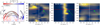 |
Fig. 10. Scenario outlining an alternative mechanism of observing downflowing RREs along a loop-like structure from a simulation perspective. Panels from left to right: a cutout of the 2D vertical velocity (vz) map focusing on the downflowing RRE formed along the loop; and λt diagrams in Ca II K, Si IV 1393 Å, and Mg II k, respectively, corresponding to the location marked with a blue dashed vertical line in the vz map (leftmost panel). The vz map corresponds to the region of interest shown in the bottom row of Fig. 2 at t = 650 s. Each of the λt diagrams show the location of Doppler shift Δλ = 0 (indicated with a white solid line), the time step (red horizontal line), and an arrow pointing at the time interval corresponding to the maximum redward excursions of the respective line centers during the evolution of the downflowing RRE. An animation of this figure is available online. |
The λt diagrams for the synthetic Ca II K, Si IV 1393 Å, and Mg II k spectral lines, corresponding to the location of the dashed vertical marker, show asymmetries toward the redward side of the respective line centers that are in tandem with the observations presented in Figs. 4–6. Moreover, the synthetic λt diagrams lack preceding blueward excursions (similar to the observed λt diagrams) that excludes them from being related to type-I spicules. A quasi-temporal redward excursion in all the three spectral lines strongly indicates that the loop-like structures observed in the chromosphere and the transition region could also lead to downflowing RREs – that are multi-thermal by nature and can be heated to 0.08 MK, similar to the spectral signatures found in the coordinated observations. Moreover, the heating associated with these loop-like downflowing RREs are found to be governed by a mechanism that is similar to examples presented in Sect. 4.3.2.
The scenario presented in this section is slightly different from the observations by Pereira et al. (2018), who found subtle or limited traces of the low-lying loops in the chromosphere. Moreover, they indicated that the footpoints of those loops were close to the footpoints of the spicules, but they were clearly distinct from one another. However, here we discussed a possibility where spicules (downflowing RREs or RBEs) are basically formed along the structure of the loop itself, and they show clear evidence of strong Doppler shifts both in the chromosphere and the transition region.
6. Concluding remarks
We study the transition region and coronal response of the recently reported downflowing RREs. Coordinated ground- and space-based observations reveal that these downflows are ubiquitous, have a multi-thermal nature with a broad temperature distribution, and can be heated to at least transition region temperatures. The downflows are most likely a result of previously heated spicular material that underwent cooling and eventually fell back into the chromosphere – a scenario that was already outlined by studies such as Pneuman & Kopp (1977), Athay (1984), and McIntosh et al. (2012). The current work provides the missing link between the abundant downflows observed in the transition region (and lower corona) with their chromospheric counterparts that had until now remained elusive. Although it is hard to estimate what fraction of the transition region redshifts are directly associated with downflowing RREs for the entire solar atmosphere, the analysis presented in this study provides a compelling case that links these observed redshifts with spicules in the chromosphere. Moreover, the Doppler shifts of the Si IV spectral line are close to the observed average redshifts found in the transition region, which leads us to believe that the downflows might play an important role in explaining the observed redshifts.
A detailed comparison with the numerical simulation from Martínez-Sykora et al. (2017a, b) successfully reproduced the observed spectral properties of the downflowing RREs to a large extent. Analysis based on contribution functions, and reinforcing the investigation of Bose et al. (2019a), shows that care should be taken when interpreting the positions of classical spectral features such as K1 and K3. Moreover, an alternate scenario has been presented from the perspective of numerical simulations that raises the possibility of observing downflowing RREs along loop-like structures and could explain the lack of preceding blueward shifts in the spectral time diagrams. It could be interesting to look for such examples in future studies from coordinated high-resolution observations from ground- and space-based facilities. We have also shown that the returning phases of type-II spicules are heated in comparison to the upflowing phases. This heating was due to a combination of various mechanisms, but ambipolar diffusion was found to play a pivotal role that led to an enhancement in the temperature by about 2−3 kK. This is further observed in the form of enhanced emission in the synthetic Ca II K and Mg II k spectra, which seems to explain the enhancement for the observed Ca II K and Mg II k spectra in the examples shown in this paper and also in Bose et al. (2019a).
Finally, we note that the effect of the nonequilibrium ionization of different atomic species, such as hydrogen, helium, and silicon, has not been included in the numerical simulation used in this paper. Nonequilibrium ionization can cause an increase in the number density of electrons in the upper chromosphere due to longer recombination timescales (Martínez-Sykora et al. 2020). Therefore, any heating (due to ambipolar diffusion, for example) will directly impact the temperature instead of ionizing and (or) recombining the plasma, producing multi-thermal structures with even sharper temperature variations (Chintzoglou et al. 2021). A detailed study including the effects of nonequilibrium ionization is currently underway and will form part of a follow-up paper.
Movies
Movie 1 associated with Fig. 1 (movie_Fig1_bottom_row) Access Supplementary Material
Movie 2 associated with Fig. 1 (movie_Fig1_top_row) Access Supplementary Material
Movie 3 associated with Fig. 2 (movie_Fig2) Access Supplementary Material
Movie 4 associated with Fig. 3 (movie_Fig3_bottom_row) Access Supplementary Material
Movie 5 associated with Fig. 3 (movie_Fig3_mid_row) Access Supplementary Material
Movie 6 associated with Fig. 3 (movie_Fig3_top_row) Access Supplementary Material
Movie 7 associated with Fig. 8 (movie_Fig8_panel_a) Access Supplementary Material
Movie 8 associated with Fig. 8 (movie_Fig8_panel_b) Access Supplementary Material
Movie 9 associated with Fig. 10 (movie_Fig10) Access Supplementary Material
The latest module for the implementation of ambipolar diffusion in the Bifrost code can be found in Nóbrega-Siverio et al. (2020).
The code is publicly available at https://github.com/ITA-Solar/rh
Acknowledgments
The Swedish 1-m Solar Telescope is operated on the island of La Palma by the Institute for Solar Physics of Stockholm University in the Spanish Observatorio del Roque de los Muchachos of the Instituto de Astrofísica de Canarias. The Institute for Solar Physics is supported by a grant for research infrastructures of national importance from the Swedish Research Council (registration number 2017-00625). IRIS is a NASA small explorer mission developed and operated by LMSAL with mission operations executed at NASA Ames Research Center and major contributions to downlink communications funded by ESA and the Norwegian Space Centre. This research is supported by the Research Council of Norway, project number 250810, and through its Centres of Excellence scheme, project number 262622, and through grants of computing time from the Programme for Supercomputing. VMJH is supported by the European Research Council (ERC) under the European Union’s Horizon 2020 research and innovation programme (SolarALMA, grant agreement No. 682462). DNS acknowledges support by the Synergy Grant number 810218 (ERC-2018-SyG) of the European Research Council, and the project PGC2018-095832-B-I00 of the Spanish Ministry of Science, Innovation and Universities. JMS gratefully acknowledges support by NASA grants 80NSSC18K1285, 80NSSC21K0737 and NNG09FA40C (IRIS). The simulations have been run on clusters from the Notur project, and the Pleiades cluster through the computing project s1061, s1630, and s2053, from the High End Computing (HEC) division of NASA. BDP is supported by NASA contract NNG09FA40C (IRIS). We are indebted to Rob Rutten for his excellent routines for alignment of SDO and ground-based data. We are thankful for the assistance of Ainar Drews with the observations of the 25 May 2017 set. We thank Pit Sütterlin for excellent SST service mode observations during the 2020 COVID-19 season. We made much use of NASA’s Astrophysics Data System Bibliographic Services. Parts of the results in this work make use of the colormaps in the CMasher package (van der Velden 2020).
References
- Antolin, P., Schmit, D., Pereira, T. M. D., De Pontieu, B., & De Moortel, I. 2018, ApJ, 856, 44 [NASA ADS] [CrossRef] [Google Scholar]
- Asplund, M., Grevesse, N., Sauval, A. J., & Scott, P. 2009, ARA&A, 47, 481 [NASA ADS] [CrossRef] [Google Scholar]
- Athay, R. G. 1984, ApJ, 287, 412 [NASA ADS] [CrossRef] [Google Scholar]
- Athay, R. G., & Holzer, T. E. 1982, ApJ, 255, 743 [NASA ADS] [CrossRef] [Google Scholar]
- Bjørgen, J. P., Sukhorukov, A. V., Leenaarts, J., et al. 2018, A&A, 611, A62 [NASA ADS] [CrossRef] [EDP Sciences] [Google Scholar]
- Bose, S., Henriques, V. M. J., Joshi, J., & Rouppe van der Voort, L. 2019a, A&A, 631, L5 [CrossRef] [EDP Sciences] [Google Scholar]
- Bose, S., Henriques, V. M. J., Rouppe van der Voort, L., & Pereira, T. M. D. 2019b, A&A, 627, A46 [NASA ADS] [CrossRef] [EDP Sciences] [Google Scholar]
- Bose, S., Joshi, J., Henriques, V. M. J., & van der Voort, L. R. 2021, A&A, 647, A147 [EDP Sciences] [Google Scholar]
- Brekke, P., Hassler, D. M., & Wilhelm, K. 1997, Sol. Phys., 175, 349 [NASA ADS] [CrossRef] [Google Scholar]
- Carlsson, M., & Leenaarts, J. 2012, A&A, 539, A39 [NASA ADS] [CrossRef] [EDP Sciences] [Google Scholar]
- Carlsson, M., & Stein, R. F. 1997, ApJ, 481, 500 [Google Scholar]
- Chintzoglou, G., De Pontieu, B., Martínez-Sykora, J., et al. 2021, ApJ, 906, 82 [CrossRef] [Google Scholar]
- Dadashi, N., Teriaca, L., & Solanki, S. K. 2011, A&A, 534, A90 [NASA ADS] [CrossRef] [EDP Sciences] [Google Scholar]
- de la Cruz Rodríguez, J., Hansteen, V., Bellot-Rubio, L., & Ortiz, A. 2015, ApJ, 810, 145 [NASA ADS] [CrossRef] [Google Scholar]
- De Pontieu, B., McIntosh, S., Hansteen, V. H., et al. 2007, PASJ, 59, S655 [Google Scholar]
- De Pontieu, B., McIntosh, S. W., Hansteen, V. H., & Schrijver, C. J. 2009, ApJ, 701, L1 [NASA ADS] [CrossRef] [Google Scholar]
- De Pontieu, B., McIntosh, S. W., Carlsson, M., et al. 2011, Science, 331, 55 [NASA ADS] [CrossRef] [Google Scholar]
- De Pontieu, B., Carlsson, M., Rouppe van der Voort, L. H. M., et al. 2012, ApJ, 752, L12 [NASA ADS] [CrossRef] [Google Scholar]
- De Pontieu, B., Title, A. M., Lemen, J. R., et al. 2014, Sol. Phys., 289, 2733 [NASA ADS] [CrossRef] [Google Scholar]
- De Pontieu, B., Martínez-Sykora, J., & Chintzoglou, G. 2017a, ApJ, 849, L7 [NASA ADS] [CrossRef] [Google Scholar]
- De Pontieu, B., De Moortel, I., Martinez-Sykora, J., & McIntosh, S. W. 2017b, ApJ, 845, L18 [NASA ADS] [CrossRef] [Google Scholar]
- Dere, K. P. 1982, Sol. Phys., 77, 77 [NASA ADS] [CrossRef] [Google Scholar]
- Dere, K. P., Landi, E., Young, P. R., et al. 2009, A&A, 498, 915 [NASA ADS] [CrossRef] [EDP Sciences] [Google Scholar]
- Doschek, G. A., Feldman, U., & Bohlin, J. D. 1976, ApJ, 205, L177 [NASA ADS] [CrossRef] [Google Scholar]
- Gebbie, K. B., Hill, F., November, L. J., et al. 1981, ApJ, 251, L115 [NASA ADS] [CrossRef] [Google Scholar]
- Gudiksen, B. V., Carlsson, M., Hansteen, V. H., et al. 2011, A&A, 531, A154 [NASA ADS] [CrossRef] [EDP Sciences] [Google Scholar]
- Hansteen, V. 1993, ApJ, 402, 741 [NASA ADS] [CrossRef] [Google Scholar]
- Hansteen, V. H., Hara, H., De Pontieu, B., & Carlsson, M. 2010, ApJ, 718, 1070 [Google Scholar]
- Henriques, V. M. J. 2012, A&A, 548, A114 [NASA ADS] [CrossRef] [EDP Sciences] [Google Scholar]
- Henriques, V. M. J., Kuridze, D., Mathioudakis, M., & Keenan, F. P. 2016, ApJ, 820, 124 [NASA ADS] [CrossRef] [Google Scholar]
- Howson, T. A., De Moortel, I., Antolin, P., Van Doorsselaere, T., & Wright, A. N. 2019, A&A, 631, A105 [CrossRef] [EDP Sciences] [Google Scholar]
- Kjeldseth-Moe, O., Brynildsen, N., Brekke, P., et al. 1988, ApJ, 334, 1066 [NASA ADS] [CrossRef] [Google Scholar]
- Kuridze, D., Henriques, V., Mathioudakis, M., et al. 2015, ApJ, 802, 26 [NASA ADS] [CrossRef] [Google Scholar]
- Langangen, Ø., De Pontieu, B., Carlsson, M., et al. 2008a, ApJ, 679, L167 [NASA ADS] [CrossRef] [Google Scholar]
- Langangen, Ø., Carlsson, M., Rouppe van der Voort, L., Hansteen, V., & De Pontieu, B. 2008b, ApJ, 673, 1194 [NASA ADS] [CrossRef] [Google Scholar]
- Leenaarts, J., Pereira, T., & Uitenbroek, H. 2012, A&A, 543, A109 [NASA ADS] [CrossRef] [EDP Sciences] [Google Scholar]
- Leenaarts, J., Pereira, T. M. D., Carlsson, M., Uitenbroek, H., & De Pontieu, B. 2013, ApJ, 772, 90 [NASA ADS] [CrossRef] [Google Scholar]
- Lemen, J. R., Title, A. M., Akin, D. J., et al. 2012, Sol. Phys., 275, 17 [Google Scholar]
- Löfdahl, M. G., Hillberg, T., de la Cruz Rodríguez, J., et al. 2021, A&A, 653, A68 [Google Scholar]
- Mariska, J. T. 1987, ApJ, 319, 465 [NASA ADS] [CrossRef] [Google Scholar]
- Martínez-Sykora, J., De Pontieu, B., Testa, P., & Hansteen, V. 2011, ApJ, 743, 23 [NASA ADS] [CrossRef] [Google Scholar]
- Martínez-Sykora, J., De Pontieu, B., Hansteen, V. H., & Gudiksen, B. 2016, ApJ, 817, 46 [NASA ADS] [CrossRef] [Google Scholar]
- Martínez-Sykora, J., De Pontieu, B., Carlsson, M., et al. 2017a, ApJ, 847, 36 [NASA ADS] [CrossRef] [Google Scholar]
- Martínez-Sykora, J., De Pontieu, B., Hansteen, V. H., et al. 2017b, Science, 356, 1269 [NASA ADS] [CrossRef] [Google Scholar]
- Martínez-Sykora, J., De Pontieu, B., De Moortel, I., Hansteen, V. H., & Carlsson, M. 2018, ApJ, 860, 116 [NASA ADS] [CrossRef] [Google Scholar]
- Martínez-Sykora, J., Leenaarts, J., De Pontieu, B., et al. 2020, ApJ, 889, 95 [CrossRef] [Google Scholar]
- McIntosh, S. W., & De Pontieu, B. 2009, ApJ, 707, 524 [NASA ADS] [CrossRef] [Google Scholar]
- McIntosh, S. W., Davey, A. R., Hassler, D. M., et al. 2007, ApJ, 654, 650 [NASA ADS] [CrossRef] [Google Scholar]
- McIntosh, S. W., Tian, H., Sechler, M., & De Pontieu, B. 2012, ApJ, 749, 60 [NASA ADS] [CrossRef] [Google Scholar]
- Nóbrega-Siverio, D., Martínez-Sykora, J., Moreno-Insertis, F., & Carlsson, M. 2020, A&A, 638, A79 [EDP Sciences] [Google Scholar]
- Pagano, I., Linsky, J. L., Valenti, J., & Duncan, D. K. 2004, A&A, 415, 331 [NASA ADS] [CrossRef] [EDP Sciences] [Google Scholar]
- Pereira, T. M. D., & Uitenbroek, H. 2015, A&A, 574, A3 [NASA ADS] [CrossRef] [EDP Sciences] [Google Scholar]
- Pereira, T. M. D., De Pontieu, B., Carlsson, M., et al. 2014, ApJ, 792, L15 [NASA ADS] [CrossRef] [Google Scholar]
- Pereira, T. M. D., Rouppe van der Voort, L., & Carlsson, M. 2016, ApJ, 824, 65 [NASA ADS] [CrossRef] [Google Scholar]
- Pereira, T. M. D., Rouppe van der Voort, L., Hansteen, V. H., & De Pontieu, B. 2018, A&A, 611, L6 [CrossRef] [EDP Sciences] [Google Scholar]
- Pesnell, W. D., Thompson, B. J., & Chamberlin, P. C. 2012, Sol. Phys., 275, 3 [Google Scholar]
- Peter, H. 1999, ApJ, 516, 490 [NASA ADS] [CrossRef] [Google Scholar]
- Peter, H., & Judge, P. G. 1999, ApJ, 522, 1148 [NASA ADS] [CrossRef] [Google Scholar]
- Pneuman, G. W., & Kopp, R. A. 1977, A&A, 55, 305 [NASA ADS] [Google Scholar]
- Rouppe van der Voort, L., Leenaarts, J., De Pontieu, B., Carlsson, M., & Vissers, G. 2009, ApJ, 705, 272 [NASA ADS] [CrossRef] [Google Scholar]
- Rouppe van der Voort, L., De Pontieu, B., Pereira, T. M. D., Carlsson, M., & Hansteen, V. 2015, ApJ, 799, L3 [NASA ADS] [CrossRef] [Google Scholar]
- Rouppe van der Voort, L. H. M., De Pontieu, B., Carlsson, M., et al. 2020, A&A, 641, A146 [EDP Sciences] [Google Scholar]
- Rutten, R. J. 2020, ArXiv e-prints [arXiv:2009.00376] [Google Scholar]
- Rutten, R. J., Rouppe van der Voort, L. H. M., & De Pontieu, B. 2019, A&A, 632, A96 [EDP Sciences] [Google Scholar]
- Samanta, T., Tian, H., Yurchyshyn, V., et al. 2019, Science, 366, 890 [CrossRef] [Google Scholar]
- Scharmer, G. B., Bjelksjö, K., Korhonen, T. K., Lindberg, B., & Petterson, B. 2003, in Innovative Telescopes and Instrumentation for Solar Astrophysics, eds. S. L. Keil, & S. V. Avakyan, SPIE Conf. Ser., 4853, 341 [Google Scholar]
- Scharmer, G. B., Narayan, G., Hillberg, T., et al. 2008, ApJ, 689, L69 [Google Scholar]
- Scharmer, G. B., Löfdahl, M. G., Sliepen, G., & de la Cruz Rodríguez, J. 2019, A&A, 626, A55 [NASA ADS] [CrossRef] [EDP Sciences] [Google Scholar]
- Sekse, D. H., Rouppe van der Voort, L., & De Pontieu, B. 2012, ApJ, 752, 108 [NASA ADS] [CrossRef] [Google Scholar]
- Sekse, D. H., Rouppe van der Voort, L., De Pontieu, B., & Scullion, E. 2013, ApJ, 769, 44 [NASA ADS] [CrossRef] [Google Scholar]
- Skogsrud, H., Rouppe van der Voort, L., & De Pontieu, B. 2014, ApJ, 795, L23 [Google Scholar]
- Skogsrud, H., Rouppe van der Voort, L., & De Pontieu, B. 2016, ApJ, 817, 124 [NASA ADS] [CrossRef] [Google Scholar]
- Sukhorukov, A. V., & Leenaarts, J. 2017, A&A, 597, A46 [NASA ADS] [CrossRef] [EDP Sciences] [Google Scholar]
- Tian, H., DeLuca, E. E., Cranmer, S. R., et al. 2014, Science, 346, 1255711 [Google Scholar]
- Uitenbroek, H. 2001, ApJ, 557, 389 [NASA ADS] [CrossRef] [Google Scholar]
- van der Velden, E. 2020, J. Open Sour. Softw., 5, 2004 [NASA ADS] [CrossRef] [Google Scholar]
- van Noort, M., Rouppe van der Voort, L., & Löfdahl, M. G. 2005, Sol. Phys., 228, 191 [Google Scholar]
- Vissers, G., & Rouppe van der Voort, L. 2012, ApJ, 750, 22 [NASA ADS] [CrossRef] [Google Scholar]
- Wood, B. E., Harper, G. M., Linsky, J. L., & Dempsey, R. C. 1996, ApJ, 458, 761 [NASA ADS] [CrossRef] [Google Scholar]
- Zacharias, P., Hansteen, V. H., Leenaarts, J., Carlsson, M., & Gudiksen, B. V. 2018, A&A, 614, A110 [CrossRef] [EDP Sciences] [Google Scholar]
All Figures
|
Fig. 1. Full FOV of the observations corresponding to data sets 1 (top row) and 2 (bottom row). Top row, panel a: Hα red wing image observed with CRISP at a Doppler offset of +40 km s−1, panel b: corresponding CHROMIS Ca II K line core image, and panels c and d: co-spatial Si IV 1400 Å SJI from IRIS and the 171 Å image from AIA, respectively. Bottom row, panel a: Hα red wing image observed at a Doppler offset of +36 km s−1 acquired with CRISP, and panels b–d: corresponding co-spatial cutouts from AIA 304 Å, the IRIS Si IV 1400 Å SJI, and AIA 171 Å, respectively. The dashed vertical lines correspond to the spatial extent of the IRIS rasters in the two data sets, and the direction to solar north is pointing upward. The white and cyan boxes in the top and bottom rows represent the area of the Ca II K core and the Hα red wing images, respectively. Animations corresponding to these figures are available online. |
| In the text | |
|
Fig. 2. Overview of the MHD simulation snapshot from Martínez-Sykora et al. (2017b) showing a 2D slice of temperature (top row) and signed vertical velocity vz (bottom row) at t = 190 s from the start. The spicules appear as cool finger-like intrusions in the hot corona, and the ones that are further analyzed are numbered 1 and 2. Velocities away from the observer are indicated in red (positive) and toward the observer in blue (negative). The contour indicates the location where the temperature equals 30 kK. The region to left of the dashed vertical line in the bottom row indicates the region of interest that is further studied in Sect. 5.3. An animation of this figure is available online. |
| In the text | |
|
Fig. 3. Space-time (X − t) diagrams for three representative downflowing RREs, on 25 May 2017 (top row) and 19 September 2020 (middle and bottom rows), showing their multi-thermal nature across multiple wavelength channels. The dashed vertical lines in the Hα red wing images indicate the region along which the X − t maps have been extracted in the coordinated SST, IRIS, and SDO data sets. The different panels in each row corresponds to the X − t maps in the different wavelength channels as indicated at the top. The solid white vertical lines in the X − t maps correspond to the time step at which these maps have been shown. Animations of this figure are available online. |
| In the text | |
|
Fig. 4. Representative example of a downflowing RRE observed in the SST, IRIS, and SDO data sets acquired on 25 May 2017 and its spectral signature across the different chromospheric and transition region spectral lines. Top row (left to right): Hα red wing image showing the downflowing RRE at +40 km s−1, X − t maps (extracted from the region bounded by the two dashed red lines) corresponding to the Hα red wing at +40 km s−1, the IRIS Si IV 1400 Å SJI, and the AIA 171 Å channels. Middle row (from left to right): λt diagrams in Hα, Ca II K, Si IV 1393 Å, and Mg II k, respectively, corresponding to the spatial location marked with a white cross in the Hα red wing image. Bottom row: corresponding spectral profiles for the different wavelengths at the instant of maximum redward excursion (magenta marker) indicated in the λt diagrams. The dashed spectral profiles correspond to the spatial and temporal average over the whole time series in each case. The observed intensity is shown in arbitrary units. |
| In the text | |
|
Fig. 5. Second representative example of a downflowing RRE observed on 25 May 2017 in the same format as Fig. 4. |
| In the text | |
|
Fig. 6. Third representative example of a downflowing RRE observed on 25 May 2017 in the same format as Fig. 4. |
| In the text | |
|
Fig. 7. Synthetic observables of the chromospheric and transition region spectral lines obtained from the numerical simulation. Top row (left to right): a cutout of the 2D temperature map, the signed vertical velocity around spicule 1, and the Ca II K, Mg II k, and Si IV 1393 Å synthetic spectra corresponding to the upflowing phase of the spicule at t = 140 s. Bottom row: corresponding temperature, vertical velocity, and synthetic spectra for the downflowing phase of the spicule at t = 370 s in the same format as the top row. Temperatures beyond 30 kK have been masked in the 2D temperature maps and are indicated with a black contour in the vertical velocity maps. The dashed vertical blue line corresponds to the LOS of the observer along which optically thick (thin) radiative transfer is performed. |
| In the text | |
|
Fig. 8. Spatio-temporal evolution of the different thermodynamic parameters obtained from the MHD simulation. The left column of panel a shows the 2D maps of temperature, internal energy, and the sum over heating parameters (as described in the text) per particle (ρ being the plasma density), and the right column indicates the space-time maps corresponding to each of the physical quantities for spicule 1. The two columns of panel b shows the spatio-temporal evolution corresponding to the same physical quantities for spicule 2, in the same format as panel a. The dashed lines in the left column of the two panels show the bounding regions that are considered for extracting the X − t maps (shown in the respective right columns), and the vertical red line in the X − t maps corresponds to the time steps at which these maps have been shown. Animations of this figure are available online. |
| In the text | |
|
Fig. 9. Intensity formation breakdown figure for the Ca II K and Mg II k spectral lines corresponding to spicule 1 from the model atmospheres at the location indicated by the vertical marker in Fig. 7. Panel a: formation of the Ca II K spectral line at t = 140 s (upflowing phase). Panel b: formation of the Ca II K spectral line at t = 370 s (downflowing phase) with a strong asymmetry toward the redward side of the line center. Panel c: formation of the Mg II k line for the upflowing phase. Panel d: formation of a single peaked Mg II k spectral line for the downflowing phase. Each sub-panel shows (dark corresponds to low values and orange corresponds to high values) the quantity indicated at the top left corner as a function of geometric height z and frequency from the line center in km s−1. The τν = 1 curve (white) and vertical velocity (yellow, positive is downflow) are overplotted in each sub-panel. The solid gray line (indicating zero Doppler shift) is shown in the first sub-panels for reference. In addition, the first sub-panels show the ionization fraction (dotted cyan line) of Ca II (panels a and b) and Mg II (panels c and d) as a function of z. The upper right sub-panels also contain the plasma temperature (dashed green) as a function of z in logarithmic scale, specified along the top. The lower right panel also shows the specific intensity profiles (cyan) as radiation temperature with units specified on the right-hand side. |
| In the text | |
|
Fig. 10. Scenario outlining an alternative mechanism of observing downflowing RREs along a loop-like structure from a simulation perspective. Panels from left to right: a cutout of the 2D vertical velocity (vz) map focusing on the downflowing RRE formed along the loop; and λt diagrams in Ca II K, Si IV 1393 Å, and Mg II k, respectively, corresponding to the location marked with a blue dashed vertical line in the vz map (leftmost panel). The vz map corresponds to the region of interest shown in the bottom row of Fig. 2 at t = 650 s. Each of the λt diagrams show the location of Doppler shift Δλ = 0 (indicated with a white solid line), the time step (red horizontal line), and an arrow pointing at the time interval corresponding to the maximum redward excursions of the respective line centers during the evolution of the downflowing RRE. An animation of this figure is available online. |
| In the text | |
Current usage metrics show cumulative count of Article Views (full-text article views including HTML views, PDF and ePub downloads, according to the available data) and Abstracts Views on Vision4Press platform.
Data correspond to usage on the plateform after 2015. The current usage metrics is available 48-96 hours after online publication and is updated daily on week days.
Initial download of the metrics may take a while.