| Issue |
A&A
Volume 653, September 2021
|
|
|---|---|---|
| Article Number | A159 | |
| Number of page(s) | 18 | |
| Section | Interstellar and circumstellar matter | |
| DOI | https://doi.org/10.1051/0004-6361/202141591 | |
| Published online | 27 September 2021 | |
Modeling accretion shocks at the disk–envelope interface
Sulfur chemistry
1
Leiden Observatory, Leiden University,
PO Box 9513,
2300
RA
Leiden,
The Netherlands
e-mail: This email address is being protected from spambots. You need JavaScript enabled to view it.
2
Max Planck Institut für Extraterrestrische Physik (MPE),
Giessenbachstrasse 1,
85748
Garching,
Germany
3
Observatoire de Paris, Université PSL, Sorbonne Université, LERMA,
75014
Paris,
France
4
Laboratoire de Physique de l’École normale supérieure, ENS, Université PSL, CNRS, Sorbonne Université, Université de Paris,
75005
Paris,
France
Received:
18
June
2021
Accepted:
18
July
2021
Abstract
Context. As material from an infalling protostellar envelope hits the forming disk, an accretion shock may develop which could (partially) alter the envelope material entering the disk. Observations with the Atacama Large Millimeter/submillimeter Array (ALMA) indicate that emission originating from warm SO and SO2 might be good tracers of such accretion shocks.
Aims. The goal of this work is to test under what shock conditions the abundances of gas-phase SO and SO2 increase in an accretion shock at the disk–envelope interface.
Methods. Detailed shock models including gas dynamics were computed using the Paris-Durham shock code for nonmagnetized J-type accretion shocks in typical inner envelope conditions. The effect of the preshock density, shock velocity, and strength of the ultraviolet (UV) radiation field on the abundance of warm SO and SO2 is explored. Compared with outflows, these shocks involve higher densities (~107 cm−3), lower shock velocities (~few km s−1), and large dust grains (~0.2 μm) and thus probe a different parameter space.
Results. Warm gas-phase chemistry is efficient in forming SO under most J-type shock conditions considered. In lower-velocity (~3 km s−1) shocks, the abundance of SO is increased through subsequent reactions starting from thermally desorbed CH4 toward H2CO and finally SO. In higher velocity (≳4 km s−1) shocks, both SO and SO2 are formed through reactions of OH and atomic S. The strength of the UV radiation field is crucial for SO and in particular SO2 formation through the photodissociation of H2O. Thermal desorption of SO and SO2 ice is only relevant in high-velocity (≳5 km s−1) shocks at high densities (≳107 cm−3). Both the composition in the gas phase, in particular the abundances of atomic S and O, and in ices such as H2S, CH4, SO, and SO2 play a key role in the abundances of SO and SO2 that are reached in the shock.
Conclusions. Warm emission from SO and SO2 is a possible tracer of accretion shocks at the disk–envelope interface as long as a local UV field is present. Observations with ALMA at high-angular resolution could provide further constraints given that other key species for the gas-phase formation of SO and SO2, such as H2S and H2CO, are also covered. Moreover, the James Webb Space Telescope will give access to other possible slow, dense shock tracers such as H2, H2O, and [S I] 25 μm.
Key words: astrochemistry / shock waves / stars: formation / stars: protostars / stars: low-mass / ISM: abundances
© ESO 2021
1 Introduction
It is currently still unknown how much reprocessing of material occurs during the collapse from a prestellar core to a protostar and disk. Two scenarios can be considered: the inheritance scenario where the chemical composition is conserved from a cloud to disk, or the (partial) reset scenario where the envelope material is modified during its trajectory from an envelope to disk. Some inheritance is suggested by the rough similarity between cometary and interstellar ices (Mumma & Charnley 2011; Drozdovskaya et al. 2018, 2019). On the other hand, some modification of envelope material is expected due to the increase in temperature and stellar ultraviolet (UV) radiation during infall (e.g., Aikawa et al. 1999; Visser et al. 2009). Moreover, as the infalling envelope hits the disk, an accretion shock may develop which can alter the composition of the material flowing into the disk, and therefore (partially) reset the chemistry. In the most extreme case, reset implies complete vaporization of all molecules back to atoms with subsequent reformation. Milder versions of reset include sputtering of ices, and gas and ice chemistry modifying abundances.
Already in the earliest Class 0 phase of the low-mass star-formation process, an accretion disk around the young protostar is formed (e.g., Tobin et al. 2012; Murillo et al. 2013). The impact of infalling envelope material onto the disk can cause a shock, raising temperatures of gas and dust at the disk–envelope interface to values much higher than from heating by stellar photons alone (Draine et al. 1983; Neufeld & Hollenbach 1994). These low-velocity (~ few km s−1) accretion shocks at high densities (~ 107 cm−3) are widely found in models and simulations (e.g., Cassen & Moosman 1981; Li et al. 2013; Miura et al. 2017), and they are often invoked in Solar System formation to explain phenomena such as noble gas trapping (Owen et al. 1992). They are most powerful in the earliest stages when the disk is still small (≲ 10 AU). However, that infalling material may eventually end up in the protostar and not in the disk. As the embedded disk reaches a size of (several) tens of AU, the envelope material entering the disk remains there and eventually forms the building blocks of planets (e.g., Harsono et al. 2018; Manara et al. 2018; Tychoniec et al. 2020).
These accretion shocks have not yet been undisputedly detected. Typical optical shock tracers such as [O I] 6300 Å and [S II] 6371 Å are more sensitive to high-velocity shocks (≳ 20 km s−1, e.g., Podio et al. 2011; Banzatti et al. 2019) and difficult to detect in protostellar environments due to the high extinction by the surrounding envelope. Observations of mid-infrared (MIR) shock tracers such as H2O, high-J CO, [S I] 25 μm, and [O I] 63 μm suffer from outflow contamination in low-spatial resolution space-based observations (e.g., Kristensen et al. 2012; Nisini et al. 2015; Rivière-Marichalar et al. 2016) and from the Earth’s atmosphere for ground-based observations; here the launch of the James Webb Space Telescope (JWST) will provide a solution. At submillimeter wavelengths, classical diagnostics of shocks include sputtering or grain-destruction products such as CH3 OH and SiO (e.g., Caselli et al. 1997; Schilke et al. 1997; Gusdorf et al. 2008a,b; Guillet et al. 2009; Suutarinen et al. 2014). However, usually these species are only observed in relatively high-velocity outflows and jets through broad emission lines (e.g., Tychoniec et al. 2019; Taquet et al. 2020; Codella et al. 2020).
Sulfur bearing species such as SO and SO2 are suggested as possible accretion shock tracers. An enhancement of warm SO emission at the centrifugal barrier, the interface between envelope and disk, is observed in the L1527 Class 0/I system with the Atacama Large Millimeter/submillimeter Array (ALMA) at ~ 100 AU scales (Sakai et al. 2014, 2017). A similar rotating structure in SO is seen toward the Class I system Elias 29 (Oya et al. 2019). Equivalently, warm SO2 emission possibly related to an accretion shock is observed toward the B335 Class 0 protostar (Bjerkeli et al. 2019) and a few Class I sources (Oya et al. 2019; Artur de la Villarmois et al. 2019). However, both SO and SO2 are also seen related to outflow activity, both in large-scale outflows (e.g., Codella et al. 2014; Taquet et al. 2020) as in disk winds on smaller scales (e.g., Tabone et al. 2017; Lee et al. 2018). Moreover, high-angular resolution observations (~ 30 AU) of the Class I source TMC1A show narrow SO emission lines coming from a ring-shaped morphology which may be linked to the warm inner envelope (Harsono et al. 2021). Emission from warm SO and SO2 is thus not an unambiguous tracer of accretion shocks; comparison to shock models is necessary to make robust conclusions.
In shocks, the gas temperature readily rises to >100 K (Draine et al. 1983; Flower & Pineau des Forêts 2003; Godard et al. 2019), enough to ignite gas-phase formation of SO and SO2 (e.g., Prasad & Huntress 1980; Hartquist et al. 1980). A key species for this is the OH radical, which is efficiently produced in shocks through the endothermic reaction between H2 and atomic oxygen, but also through photodissociation of H2O. The OH radical reacts with atomic sulfur to form SO and subsequently to form SO2. Moreover, SO can also be formed from the SH radical reaction with atomic oxygen (Hartquist et al. 1980). Since the gas-phase chemistry of SO and SO2 in shocks is dependent on radicals such as OH and SH, the abundance of these species is not solely determined through the temperaturein the shock but also through the strength of the local UV field.
Alternatively, thermal desorption of SO and SO2 ice in shocks can enhance the gas-phase abundances of SO and SO2. In interstellar ices, OCS is the only securely identified sulfur-bearing species (Geballe et al. 1985; Palumbo et al. 1995), with a tentative detection for SO2 (Boogert et al. 1997; Zasowski et al. 2009). It is suggested that H2S is the main sulfur carrier in the ices (e.g., Vidal et al. 2017), but so far only upper limits could be derived (Jiménez-Escobar & Muñoz Caro 2011). To date, SO ice has not yet been detected. All aforementioned species are observed in cometary ices such as 67P/Churyumov-Gerasimenko (Calmonte et al. 2016; Rubin et al. 2019; Altwegg et al. 2019). Miura et al. (2017) modeled low-velocity (2 km s−1) accretion shocks taking into account the dust dynamics but without any gas-phase chemistry included and could only explain the observationsof Sakai et al. (2014) if SO was thermally desorbed while adopting dust grains that were smaller than 0.1 μm. Sputtering seems to be irrelevant as this becomes only efficient at larger shock velocities (> 10 km s−1; e.g., Aota et al. 2015). However, to thermally desorb sulfur-bearing ices such as SO and SO2 from the grains, the dust temperature has to reach values on the order of 40–70 K.
In this paper, we present a grid of irradiated low-velocity (< 10 km s−1) J-type accretion shock models at typical inner envelope densities (105 –108 cm−3). This is a different parameter space than usually explored in, for example, higher-velocity (> 10 km s−1) outflows at lower densities (~ 104 cm−3). The goal is to test under what shock conditions the abundance of warm SO and SO2 is significantly increased. In Sect. 2, the model and input parameters are introduced. We present the results of our analysis in Sect. 3, after which we discuss these results in Sect. 4. Our conclusions are summarized in Sect. 5.
2 Accretion shock model
2.1 Shock model
The accretion shock at the disk–envelope interface is modeled using a slightly modified version of the Paris–Durham shock code (Flower & Pineau des Forêts 2003; Lesaffre et al. 2013; Godard et al. 2019). This publicly available numerical tool1 computes the dynamical, thermal, and chemical structure of stationary plane parallel shock waves. The models therefore represent a continuous inflow of envelope material onto the disk and thus a continuous sequence of shocks. The location of the accretion shock is expected to move outward as the disk grows and evolves (Visser & Dullemond 2010).
In this paper, only stationary nonmagnetized J-type accretion shocks are presented. The presence of a magnetic field can result in C or CJ-type shocks (e.g., Draine 1980; Flower & Pineau des Forêts 2003), see Appendix E for details. However, the length of C-type accretion shocks is strongly dependent on the initial conditions and the size of dust grains and may reach envelope scales of ~ 1000 AU, which is not consistent with the emission of SO and SO2 seen on <100 AU scales (e.g., Sakai et al. 2014, 2017; Artur de la Villarmois et al. 2019; Oya et al. 2019). CJ-type shocks could be relevant in intermediate magnetized inner envelopes (~ 0.1 mG; Hull et al. 2017, Appendix E), but to compute CJ-type shocks across our specific parameter space (low velocities, high densities), the Paris-Durham code needs to be tuned, which is beyond the scope of this work. Nevertheless, the results of CJ and C-type shocks are not expected to be different from J-type shocks in terms of chemistry.
In the following sections, the main physical and chemical quantities and properties that are included in the model are introduced. In particular, the most relevant physical and chemical processes and updates on the version of the code presented by Godard et al. (2019) are highlighted.
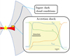 |
Fig. 1 Physical structure of a protostellar envelope. Starting with dark cloud conditions, an accretion shock model is calculated. The shock profile in the bottom panel is shown on a logarithmic scale with the yellow region indicating the shocked region. |
2.1.1 Geometry
The shock iscalculated following a stationary plane parallel structure, see Fig. 1. A shock front propagates with a velocity Vs in the direction of negative distance z. The entire structure is irradiated with an isotropic radiation field equal to the isotropic standard interstellar radiation field (ISRF) scaled with a factor G0 (Mathis et al. 1983), as was implemented by Godard et al. (2019). In protostellar systems, the UV radiation can originate both from the accretion onto the protostar itself or from shocks in the bipolar jets (e.g., van Kempen et al. 2009; Y"i"ld"i"z et al. 2012; Benz et al. 2016). Moreover, the extinction AV between the source of UV irradiation and the shock at the disk–envelope interface can be as high as ~ 10 mag (e.g., Drozdovskaya et al. 2015) and is assumed to be taken into account with the choice of G0. Therefore, the exact source of UV radiation is irrelevant here as long as a reasonable range in G0 is covered and since the radiation field is assumed to be isotropic. A diluted black body of 100 K representing far-infrared (FIR) dust emission from the accretion disk is added to the radiation field. Assuming an emitting region of 4.5 AU at a distance of 100 AU, the black body is diluted with a factor W = 5 × 10⁻⁴ (for details, see Appendix A of Tabone et al. 2020) and is constant for all models. Additionally, secondary UV photons created through the collisional excitation of H2 by electrons produced by cosmic ray ionization are included.
2.1.2 Radiative transfer and photon processes
Photodissociation and photoionization processes of both the gas and dust are taken into account. The cross sections are taken from the Leiden database (Heays et al. 2017). To save computation time, the photoreaction cross sections were only used for the photodissociation of CH, CH3, CH4, NH, CN, O2, OH, H2O, H2CO, SH, H2S, CS, OCS, SO, and SO2, and the photoionization of C, S, CH, CH3, CH4, O2, OH, H2O, H2CO, SH, H2S, and SO. Photodissociation and photoionization of all other species are also included in the chemistry using the analytical expression of Heays et al. (2017). Due to the self-shielding properties of H2, CO, and N2, photodissociation of these species is assumed to be negligible. The destruction of atoms and molecules by far-ultraviolet photons between 911 Å and 2400 Å is calculatedincluding both continuum and discrete processes.
2.1.3 Grains and PAHs
The grains are assumed to have grown in protostellar envelopes to larger sizes than the typical interstellar medium (ISM) distribution (e.g., Guillet et al. 2007; Miotello et al. 2014; Harsono et al. 2018; Galametz et al. 2019). Here, we assume that all grains have an initial core size of 0.2 μm (Guillet et al. 2020) and are either neutral, single negatively, or single positively charged. Moreover, the dust grains are assumed to be dynamically coupled to the gas. Grain-grain interactions are not included since vaporization and shattering of dust grains are only relevant for J-type shocks moving at high velocities (> 20 km s−1; Guillet et al. 2009). Dust coagulation can potentially be relevant in changing the grain size distribution (Guillet et al. 2011, 2020) but is not included here.
Other large species are polycyclic aromatic hydrocarbons (PAHs), which are modeled here as single particles with a size of 6.4 Å (Flower & Pineau des Forêts 2003). In most studies of interstellar shocks, the abundance of PAHs is set to the typical value of the ISM (~ 10−6 with respect to the proton density nH = 2n(H2) + n(H) + n(H+); Draine & Li 2007). However, given that PAHs freeze out in dense clouds, the abundance of PAHs in the gas is set to ~ 10−8 with respect to nH (Geers et al. 2009).
2.1.4 Chemical network
The chemical network adopted in this work consists of 143 species which can take place in about a thousand reactions, both in the gas phase and in the solid state. The network is largely similar to that used by Flower & Pineau des Forêts (2015) and Godard et al. (2019) with the addition of important sulfur bearing ices such as SO and SO2 and their desorption and adsorption reactions. Moreover, the binding energies of all ice species were updated (e.g., 1800 K, 3010 K, and 2290 K for SO, SO2, and H2S, respectively; Penteado et al. 2017). For a density of 108 cm−3, this results in a sublimation temperature of 37 K, 62 K, and 47 K for SO, SO2, and H2S, respectively.For simplicity, grain surface reactions have been disabled since the effect of these reactions ontimescales of the shock is negligible. Sputtering of ices is not relevant here since in J-type shocks all material is coupled in one fluid.
2.1.5 Heating and cooling
The thermal balance is calculated consistently throughout the shock. The main sources of gas heating in nonmagnetized J-type shocks are through viscous stresses and compression of the medium at the shock front where Tgas increases adiabatically over a few mean free paths. A second form of heating occurs through irradiation coming from the incident local UV radiation field and through gas-dust thermal coupling.
The gas is cooled through atomic lines of C, N, O, S, and Si, ionic lines of C+, N+, O+, S+, and Si+, and rotational and rovibrational lines of H2, OH, H2O, NH3, 12CO, and 13CO (Flower & Pineau des Forêts 2003; Lesaffre et al. 2013; Godard et al. 2019). All cooling by atomic and ionic lines as well as rovibrational lines of H2 are calculated in the optically thin limit. The cooling of OH is calculated using an analytical cooling function (Le Bourlot et al. 2002), which holds up to densities of 1010 cm−3. However, for NH3, local thermodynamic equilibrium (LTE) effects become relevant already for densities ≳ 108 cm−3. The cooling through pure rotational lines of NH3 has therefore been recalculated numerically using the RADEX software (van der Tak et al. 2007) in the optically thin limit, see Appendix A. Cooling by rovibrational lines of H2O, 12CO, and 13CO is computed using the tabulated values of Neufeld & Kaufman (1993) which take into account opacity effects. Additionally, the gas can be cooled though collisions with dust grains which subsequently radiate away the heat.
The temperature of the dust is calculated from the equilibrium between heating through absorption of photons, thermal collisions with the gas which can both heat and cool the dust, and cooling through infrared emission (Godard et al. 2019). The FIR radiation field of the 100 K black body is of particular importance for the heating for dust grains in the pre and postshock regimes as it sets a minimum dust temperature of ~ 22 K. A dust temperature of < 20 K implies that even the most volatile species such as CO and N2 are frozen out onto dust grains. However, observations of embedded protostellar systems suggest that CO and N2 are not frozen out in the inner regions of such systems (e.g., van ’t Hoff et al. 2018). A higher dust temperature would result in more ice species being desorbed prior to the shock but the effect on the shock structure and chemistry is negligible.
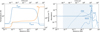 |
Fig. 2 Left: temperature and density structure in the fiducial J-type shock. The shock starts at 0 AU and ends at about 5 AU. The dust temperature does not increase enough for thermal sublimation of SO and SO2. Right: abundance profiles of SO (solid) and SO2 (dashed) and the key species for gas-phase formation of these species: SH (dot-dashed) and OH (dotted). The region where Tgas >50 K is indicated with the shaded blue region. |
Fiducial model parameters and explored parameter range.
2.2 Input parameters
The range of physical parameters explored in this paper is presented in Table 1. Important physical parameters are the initial proton density nH, the cosmic ray ionization rate of H2  , the strength of the local incident radiation field, and the shock velocity Vs. Depending on the mass of the source and size of the disk, the density of infalling envelope material impacting the disk can be ~ 105–108 cm−3 (e.g., Harsono et al. 2015). Therefore, the investigated range of nH covers ~ 105–108 cm−3, with the fiducial value at 107 cm−3. The radiation field is parameterized as a combination of the ISRF multiplied with a factor G0 (Mathis et al. 1983)and infrared emission from the disk (which is constant for all models). The strength of the local UV radiation field at the disk–envelope interface is highly uncertain and (among other things) dependent on the distanceto the source of UV radiation (see Sect. 2.1.1). Without extinction the local G0 value could be as high as 104 at ~100 AU (Visser et al. 2012). However, taking into account the extinction the local strength will likely not be much higher than a G0 of ~ 100. Therefore, a large range in G0 is considered: 10−3–102, with a fiducial value of G0 = 1. The fiducial Vs is set to 3 km s−1, which is roughly equal to the velocity of the infalling envelope at 100 AU for a 0.5 M⊙ star. Shock velocities of 1–10 km s−1 are considered, which correspond to an infalling envelope at 10–1000 AU. The initial gas temperature is set to 25 K.
Input abundances of smaller molecules and atoms are set to match typical low-mass dark cloud conditions (van der Tak et al. 2003; Boogert et al. 2015; Navarro-Almaida et al. 2020; Tafalla et al. 2021; Goicoechea & Cuadrado 2021). The initial gas-phase abundance of atomic S and O is set to 10−6 with respect to nH, with most of the oxygen and carbon reservoirs locked up in refractory grain cores or ices such as H2O and CH4 (10−4 and 10−6, respectively; Boogert et al. 2015). The dominant sulfur carrier is assumed to be H2S ice with an abundance of ~2 × 10⁻⁵ (e.g., Vidal et al. 2017; Navarro-Almaida et al. 2020). The abundance of both SO and SO2 ice was set to 10−7 (e.g., Boogert et al. 2015; Rubin et al. 2019; Altwegg et al. 2019), with the initial gas-phase abundance at 10−9 (van der Tak et al. 2003). The full list of input abundances is presented in Appendix B.
3 Results
3.1 Temperature and density
The gas and dust temperature, Tgas and Tdust, respectively,and density structure of the fiducial shock model are shown in the left of Fig. 2. At the start of the shock, Tgas increases to ~500 K, which is in agreement with the analytic expression for a weakly magnetized and fully molecular shock derived by Lesaffre et al. (2013) from the Rankine-Hugoniot relations,
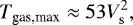 (1)
(1)
where Vs is the initial shock velocity in units of km s−1. Following the jump in temperature, the gas is cooled down through radiation of rotational and rovibrational molecular lines and atomic lines. The most dominant coolant right after the shock front is H2, while cooling by (optically thick) pure rotational and rovibrational lines of CO and H2O takes over as the temperature drops below ≲400 K. Cooling of the gas through gas-dust thermal coupling is negligible. Cooling through NH3 in the optically thin limit is significant for shocks with Vs ≳ 6 km s−1 since in those shocks the abundance of NH3 is significantly increased through high-temperature gas-phase chemistry. The end of the shock is defined as the distance where Tgas drops below 50 K, which corresponds to ~3 AU for the fiducial model. In the postshock, the thermal balance between gas and dust is determined by heating of the dust through the FIR radiation field, gas-grain collisions that transfer the heat from dust to gas, and cooling of the gas through predominantly CO rotational transitions.
The dust temperature is very relevant for these shocks since it increases to values where thermal desorption of ices occurs. In the shock, the material compresses, increasing the density by up to two orders of magnitude (i.e., to about 109 cm−3 in Fig. 2). Due to the thermal coupling between the gas and dust, Tdust increases to ~30 K for the fiducial model, enough for thermal sublimation of volatile species such as CH4 but not for more strongly bound ices such as H2S, H2O, and CH3OH. However, as shown in Fig. 3, Tdust can become as large as >70 K in the highest-velocity (~ 10 km s−1) shocks in the densest (108 cm−3) media, resulting in thermal sublimation of several ices including H2S, SO, and SO2. Dust heating through UV radiation is only significant for strongest irradiated environments with G0 ≳ 50 and only up to Tdust ≲ 25 K. Since photodesorption of ices is negligible on timescales of the shock (see Eq. (C.2)), thermal desorption is the dominant mechanism in releasing ices to the gas phase.
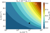 |
Fig. 3 Maximum dust temperature reached (in color) in shock models as function of initial nH and Vs. All other physical parameters are kept constant to the fiducial values and listed on top of the figure. The black cross indicates the position of the fiducial model. |
3.2 Chemistry of SO and SO2
The abundance profiles of SO and SO2 in the fiducial model are presented in the right part of Fig. 2. Toward the end of the shock, as the gas and dust are cooling down, a significant increase in the abundances of SO is visible up to the ~ 5 × 10⁻⁸ level. The abundance of SO2 does not increase above the dark cloud abundance of 10−9 (van der Tak et al. 2003). The maximum abundance reached in the shock for SO and SO2 as function of different initial nH and Vs is presented inFig. 4. In the following subsections different parts of the parameter space are highlighted using the relevant chemical formation pathways in Fig. 5.
3.2.1 Low-velocity shocks: ~ 3 km s−1
In low-velocity (~ 3 km s−1) shocks, thermal desorption of SO and SO2 ice does not occur since Tdust only rises to ≲35 K. Any increase in abundance thus originates from gas-phase chemistry. Here, the relevant chemical reaction leading to the formation of SO is,
 (2)
(2)
The main formation pathway here of SH is via the green route of Fig. 5, that is, through the reaction of H2CO with S+. Since H2CO only desorbs directly from the ice when Tdust ≳ 65 K, H2CO is formed through the gas-phase reaction of the CH3 radical with atomic O. To get a significant amount of CH3 in the gas, CH4 ice needs to desorb (at Tdust ≳ 25 K; Penteado et al. 2017) and subsequently photodissociate into CH3 and atomic H. The S+ ion originates from the photo-ionization of atomic S. The strongest increase in abundance through this route is at intermediate densities (nH~ 107 cm−3). It is important to note that H2CO is a representative here of any hydrocarbon reacting with S+ to form SH.
Some SO2 is also formed in low-velocity shocks through a reaction of SO with OH (see Reaction (4)). However, the abundance of SO2 does not increase above the initial dark cloud abundance of 10−9 because no significant amount of OH is available at these shock velocities.
3.2.2 High-velocity shocks: > 4 km s−1
For shocks propagating at higher velocities (≳ 4 km s−1), both SO and SO2 are efficiently formed through gas-phase chemistry, see Fig. 4. After the start of the shock, H2O is readily formed through reactions of OH with H2 (Flower & Pineau des Forêts 2010, see also Fig. D.1). As the shock cools down to below ≲ 300 K, the production of H2O stops, but OH is still being formed through photodissociation of H2O. This increases the OH abundance in the gas which stimulates the formation of SO and SO2 through the red route of Fig. 5,

The highest abundances are achieved in less dense environments (≲ 106 cm−3), with the maximum abundance of both SO and SO2 dropping when moving toward intermediate densities (~ 106–107 cm−3). In the latter conditions, NH3 becomes a dominant coolant in the tail of the shock. Therefore, the shock cools down more quickly and hence the region of favorable conditions for SO and SO2 formation (100 ≲ Tgas ≲ 300 K) is reduced and their maximum abundances are lower.
At the highest densities (nH > 107 cm−3), thermal desorption of sulfur-bearing ices becomes relevant for the chemistry (i.e., the blue route in Fig. 5). Thermal sublimation of SO ice occurs as the dust temperature reaches ~ 37 K, leading to a strong increase in its gas-phase abundance (see Fig. 4). Thermal desorption of SO2 only happens in the highest velocity shocks in the densest media. However, desorption of H2S ice (at Tdust ~ 47 K) is also relevant for the gas-phase chemistry as subsequent photodissociation and reactions with atomic H lead to an increased abundance of SH and atomic S (i.e., the yellow route of Fig. 5).
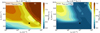 |
Fig. 4 Maximum abundance reached (in color) of SO (left) and SO2 (right) in shock models as function of initial nH and Vs. All other physical parameters are kept constant to the fiducial values and listed on top of the figure. The black cross indicates the position of the fiducial model. The dashed black line shows the ice line, i.e., where 50% of the ice is thermally desorbed into the gas in the shock. |
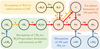 |
Fig. 5 Chemical reactions leading to the formation of gas-phase SO and SO2. Species denoted as s-X are located in the ice mantles of dust grains. Reverse reactions are not shown for clarity. Red arrows denote chemical reactions with the annotated species, yellow arrows photodissociation reactions, and blue arrows ice desorption via either thermal or nonthermal mechanisms. Relevant chemical pathways are highlighted with a colored background. |
3.2.3 Dependence on UV radiation field
As shown in Reactions (2)–(4) and Fig. 5, gas-phase formation of SO and SO2 is dependent on radicals such as OH and SH. These radicals can be created in various ways, including high-temperature chemical reactions (Prasad & Huntress 1980; Hartquist et al. 1980). However, a more dominant physical process for enhancing the abundance of OH and SH is the photodissociation of H2O, H2S, and interestingly also CH4. This process is dependent on the strength of the local UV radiation field, which is parametrized here with G0.
In Fig. 6, the maximum abundance of SO as function of Vs and nH is presented for G0 = 10−2. Similar figures of both SO and SO2 for various G0 are presented in Appendix D.2. Decreasing the strength of the UV field decreases the amount of SO and SO2 produced in high-velocity (≳ 4 km s−1) shocks due to less OH being produced through H2O photodissociation. On the other end, increasing G0 shifts the spot for efficient SO and SO2 formation in the shock to higher densities to create the favorable conditions for their chemistry. Moreover, for G0 ≳ 10, photodissociation of thermally desorbed H2S (i.e., when nH ≳ 107 cm−3 and Vs ≳ 4 km s−1) significantly increases the abundance of atomic S (i.e., yellow route of Fig. 5) which leads to an increase in abundances of SO and in particularSO2 (see Fig. D.3).
At lower shock velocities (Vs ≲ 4 km s−1), water is not formed in the shock and hence photodissociation of H2O does not increase the abundance of SO and SO2. The increase in the SO abundance is here due to the green route of Fig. 5, which isinitialized by thermal desorption and subsequent photodissociation of CH4. This formation route is most relevant for G0 = 1; for lower G0, the UV radiation field is not strong enough to photodissociate significant amounts of CH4. For higher G0, higher densities are required for the efficient production of SO through the green route.
3.2.4 Dependence on initial conditions
The abundances of all species reached in the shock, including SO and SO2, are dependent on the initial abundances. The interstellar ice abundances of SO and SO2 are not well known, with only a tentative detection for SO2 (Boogert et al. 1997; Zasowski et al. 2009). Here, the ice abundances of SO and SO2 are estimated at the 10−7 level based on what is found in cometary ices (Calmonte et al. 2016; Rubin et al. 2019; Altwegg et al. 2019). However, they are only relevant in the shocks where thermal desorption of these ices occurs (i.e., the blue route of Fig. 5 and to the right of the dashed line in Fig. 7). For those shocks, increasing or decreasing the ice abundances with an order of magnitude will also result in an increase or decrease in the gas-phase abundances with an order of magnitude, given that the ice abundance is dominant over what is achieved through gas-phase chemistry alone.
For shocks where the abundance of SO and SO2 is mainly increased through gas-phase chemistry (i.e., to the left of the dashed line in Fig. 7), the maximum abundance reached is mostly directly dependent on the initial abundance of atomic sulfur. To test the effect of initial atomic S abundance on the maximum abundances of SO and SO2, shock models are calculated for a lower gas-phase atomic sulfur abundance (low-S: XS = 10−8) and assuming that almost all sulfur is atomic and in the gas phase (high-S: XS = 2 × 10⁻⁵). The initial abundances for these cases are presented in Table 2. The resulting maximum SO and SO2 abundances for these models are shown in Fig. 7.
In the low-S case, the maximum abundance of SO drops for both low and high velocity shocks (excluding higher densities where the abundance is increased through thermal ice sublimation). This is straightforward to interpret since both S and S+ are main formation precursors of SO in both the red and green formation routes of Fig. 5, respectively. At lower densities (≲ 106 cm−3), the maximum SO2 abundance drops in a similar way since less SO is formed. However, at intermediate densities (~ 107 cm−3), slightly more SO2 is formed in high velocity shocks compared to Fig. 4. This is because atomic S and SO are “competing” to react with OH to form respectively SO and SO2. Dropping the initial atomic S abundance results in more SO2 being formed, also because the majority of the gas-phase SO here originates from thermal ice sublimation.
In the high-S case, not only the chemistry but also the thermal structure of the shock is slightly altered since cooling through atomic S becomes significant. Furthermore, more SO is formed through both the red and green routes of Fig. 5. Interestingly, the maximum abundance of SO2 attained decreases compared to Fig. 4 since with more atomic S in the gas phase to react with OH, less OH is available to react with SO toward SO2.
The initial abundances of other species are also important for the chemistry of SO and SO2. Increasing or decreasing the amount of atomic oxygen results in respectively more or less OH and H2O formed in the shock and thus directly affects the abundances of SO and SO2. Moreover, reactions with atomic carbon are a main destruction pathway for SO (forming CS; Hartquist et al. 1980). Hence an increased initial atomic carbon abundance results in lower abundances of both SO and SO2 in the shock.
In reality, the initial dark cloud abundances may also be altered during the infall from the envelope toward the disk since both the temperature and the strength of the UV radiation field increase (e.g., Aikawa et al. 1999; Visser et al. 2009; Drozdovskaya et al. 2015). To take this into account, a preshock model should be calculated. In Appendix C, the effect of calculating such a preshock model on the abundance of SO attained in the shock is presented. Any alterations on the preshock conditions are only important for the chemistry of SO and SO2 if the timescale over which the preshock is calculated is longer than about 10% of the photodesorption timescale. For typical infalling envelopes, this is not expected to be relevant.
Input abundances of key sulfur-bearing species.
3.3 Effect of grain size and PAHs
The size of the dust grains has an effect on both the physical structure of the shock and on the chemistry (e.g., Guillet et al. 2007; Miura et al. 2017). In Fig. 8, the abundance profiles of SO and SO2 are shown for the fiducial model and for the same model while adopting a typical ISM grain size distribution (computed using a single size of ~ 0.03 μm; Mathis et al. 1977; Godard et al. 2019). The decrease in grain size leads to stronger coupling between gas and dust and thus to a slightly higher dust temperature(~35 K against ~30 K for 0.2 μm grains). Moreover, the increased gas-grain coupling results in the dust being a dominant coolant in the tail of the shock, reducing the length of the shock (~1 AU against ~3 AU for the fiducial model). Nevertheless, the abundance of SO is increased in the shock but the maximum abundance reached is about a factor of 2–3 lower compared to the fiducial model. No significant increase is seen for SO2. Miura et al. (2017) found that the dust temperature easily reaches ~50 K in low-velocity shocks taking into account dust aerodynamics for ISM-size dust grains. The full treatment of dust physics, including aerodynamic heating and grain-grain interactions (Guillet et al. 2007, 2009, 2011, 2020; Miura et al. 2017), will likely move the ice line of Fig. 4 toward lower nH and Vs. However, this is beyond the scope of this work.
Contrary to dust grains, the effect of PAHs on the physical structure of J-type shocks is negligible since PAHs do not contribute to the cooling and only little to the heating if a strong UV field is present. However, PAHs do play a key role in the ionization balance and are therefore highly relevant for the chemistry (Flower & Pineau des Forêts 2003). In Fig. 8, the abundances of SO and SO2 are also shown for the fiducial model with a PAH abundance of 10−6 (equal to the value derived in the local diffuse ISM; Draine & Li 2007). The maximum abundance of SO is a factor 3–4 lower when the abundance of PAHs is at the ISM level because the PAHs are dominating the ionization balance. Consequently, the abundance of other ions, include S+, drops by more than an order of magnitude. Given that the green route of Fig. 5 is the dominant SO formation route here and dependent on S+, less SO and subsequently SO2 are formed. For high-velocity shocks, this effect is not apparent since Reactions (3) and (4) dominate the formation of SO and SO2 and are independent of ions.
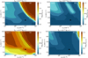 |
Fig. 7 Maximum abundance reached (in color) of SO (left) and SO2 (right) in shock models as function of initial nH and Vs for an initial gas-phase atomic S abundance of 10−8 (top row) and 10−5 (bottom row). All other physical parameters are kept constant to the fiducial values and listed on top of the figure. The black cross indicates the position of the fiducial model. The dashed black line shows the ice line, i.e., where 50% of the ice is thermally desorbed into the gas in the shock. |
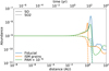 |
Fig. 8 Abundance profile of SO (solid) and SO2 (dashed) for the fiducial model (blue) with a PAH abundance of 10−8 using a grainsize of 0.2 μm. Overplotted are the same model using a typical ISM grain size of 0.03 μm (orange) anda model with a PAH abundance of 10−6 (green). All other parameters are kept at their fiducial value (see Table 1). |
3.4 Other molecular shock tracers: SiO, H2O, H2S, CH3OH, and H2
Other classical molecular shock tracers include SiO, H2O, H2S, CH3OH, and H2. Abundance maps similar to Fig. 4 of SiO, H2O, H2S, and CH3OH are presented in Appendix D.1. SiO is a tracer of shocks with significant grain destruction since then the silicon which is normally locked in dust grains can react with the OH radical to form SiO (e.g., Caselli et al. 1997; Schilke et al. 1997; Gusdorf et al. 2008a,b; Guillet et al. 2009). It is often observed in the high velocity bullets of jets originating from young Class 0 protostars (e.g., Guilloteau et al. 1992; Tychoniec et al. 2019; Taquet et al. 2020). However, the abundance of SiO is not significantly increased in our shock models because most of the Si remains locked up in silicates in the dust grains.
Water is the most abundant ice in protostellar envelopes (Boogert et al. 2015; van Dishoeck et al. 2021), but also frequently observed in outflow shocks (e.g., Flower & Pineau des Forêts 2010; Herczeg et al. 2012; Kristensen et al. 2012; Nisini et al. 2013; Karska et al. 2018). Here, H2O is efficiently produced in shocks with Vs ≳ 4 km s−1 (see Fig. D.1) and very important for the gas-phase chemistry of SO and SO2. Thermal desorption of H2O is negligible.
The main sulfur carrier in ices is suggested to be H2S (e.g., Vidal et al. 2017), despite it being undetected thus far (Jiménez-Escobar & Muñoz Caro 2011). In the gas phase, it is generally observed close to Class 0 protostars where the emission may originate from thermal desorption (Tychoniec et al. 2021), or in outflow shocks (e.g., Holdship et al. 2016). In our shock models, gas-phase formation of H2S becomes efficient at slightly higher velocities than for water (Vs ≳ 5 km s−1, see Fig. D.1). Moreover, for high-velocity shocks in dense media, H2S ice is thermally sublimated.
Methanol is a tracer of lower-velocity (< 10 km s−1) outflow shocks where ices are sputtered off the dust grains (e.g., Suutarinen et al. 2014). However, since sputtering is not relevant in our single-fluid J-type accretion shock models, no significant increase in the CH3OH abundance is evident except at the highest densities (≳ 108 cm−3) and velocities (≳ 10 km s−1) where CH3OH ice thermally sublimates.
Emission from warm H2 is generally observed toward shocks in protostellar jets (e.g., McCaughrean et al. 1994). Contrary to the molecules discussed above, the abundance of H2 remains constant along the shock and only thermal excitation occurs. Hence, H2 can be a powerful diagnostic of accretion shocks in inferring the temperature from a rotational diagram. The population of the lowest 50 rotational and rovibrational levels of H2 are computed during the shock (Flower & Pineau des Forêts 2003). The rotational diagram of H2 for the fiducial model is presented in Fig. 9. Since the temperature in this shock reaches about ~ 500 K, levels up to ~ 6000 K are collisionally populated. The population of all higher-Eup levels is set during the formation of H2 on the dust grains following a Boltzmann distribution at 17 248 K (1/3 of the dissociation energy of H2; Black & van Dishoeck 1987). Using the rotational diagram of Fig. 9, a rotational temperature ~ 390 K is derived for this shock.
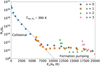 |
Fig. 9 Rotational diagram of H2 created from the fiducial shock model. The levels of different vibrational states are indicated with different symbols and colors. Only the pure rotational levels with Eu ∕kB≲ 6000 K are collisionally populated. The fit to the pure rotational levels is shown in gray line with the derived rotational temperature annotated. |
4 Discussion
4.1 Comparison to SO and SO2 with ALMA
Emission of warm (Tex > 50 K) SO and SO2 around the disk–envelope interface has been suggested as a possible tracer of accretion shocks (Sakai et al. 2014, 2017; Bjerkeli et al. 2019; Oya et al. 2019; Artur de la Villarmois et al. 2019). Here, we have shown that the abundance of both SO and SO2 can increase in shocks in typical inner envelope conditions. The abundance of SO is estimated to be ~ 10−8 in the suggested accretion shock around the L1527 Class 0/I protostar (Sakai et al. 2014), but this is uncertain since the density of H2 was guessed. Furthermore, by itself this does not provide strong constraints on the physical conditions of the shock (see Fig. 4), other than that a weak UV field should be present if SO ice is not thermally sublimated (G0 > 10−2; Fig. D.2). However, it remains difficult to derive abundances with respect to nH from observations.
Recent ALMA observations show that the amount of warm SO2 seems to increase with the bolometric luminosity (i.e., stronger UV field; Artur de la Villarmois et al. 2019). This is in line with our results since the abundance of SO2 only increases when a significant UV field is present (i.e., G0 ≳ 1, see Fig. D.3). Especially for higher velocity shocks (> 4 km s−1) at higher densities (> 107 cm−3) the maximum abundance of SO2 increases with 2 orders of magnitude between G0 = 1 and G0 = 100. However, besides a significant UV field, a shock velocity of Vs ≳ 4 km s−1 is necessary to increase the abundance of SO2 and the maximum abundance reached in the shock is also dependent on the initial density nH.
Comparing the ratio of observed column densities to those derived from our shock models can more accurately constrain the physical conditions in a shock. In Fig. 10, the column density ratio of SO2/SO in the shock is presented as function of Vs and nH for G0 = 1 and G0 = 100. The only protostellar source where both SO and SO2 have been detected related to a possible accretion shock is Elias 29 (Oya et al. 2019), where a column density ratio of  is derived. When G0 = 1, this would imply a low-density shock (< 106 cm−3) propagating at either low (< 2 km s−1) or high (> 7 km s−1) velocities, see upper panel in Fig. 10. For G0 = 100, shocks propagating at higher velocities (> 4 km s−1) at high densities (> 107 cm−3) produce SO2/SO column density ratios similar to that of Elias 29 (Oya et al. 2019, see lower panel in Fig. 10).
Since both SO and SO2 emission is also linked to outflow activity and passive heating in the inner envelope (Codella et al. 2014; Tabone et al. 2017; Lee et al. 2018; Taquet et al. 2020; Harsono et al. 2021), high spatial resolution observations with ALMA are necessary to both spatially and spectrally disentangle the different protostellar components and determine their emitting area. Moreover, to robustly test if the SO and SO2 emission traces the accretion shock, key species for their gas-phase formation such as H2S and H2CO should be observed on similar scales. This also allows for more accurately constraining the physical conditions of a shock.
4.2 Predicting H2, H2O, and [S I] with JWST
With the launch of JWST, near-infrared (NIR) and MIR shock tracers such as H2, H2O, and [S I] can be used to search for accretion shocks. Although the abundance of H2 does not increase in accretion shocks, it is still thermally excited and therefore a good shock tracer at NIR and MIR wavelengths (e.g., McCaughrean et al. 1994). Observing the rotational sequence of H2 in the NIR and MIR could thus put constraints on the physical properties of the shock. For low-velocity shocks (≲ 5 km s−1), most of the strong H2 transitions (i.e., 0-0 S(3) and 0-0 S(5)) are located in the JWST/MIRI range (5− 28 μm). For higher velocity shocks (≳ 5 km s−1), also vibrational levels of H2 get populated and the strongest H2 transitions shift toward the NIRSpec range of JWST (1− 5 μm).
Warm water is also a well-known and important tracer of shocks (e.g., Herczeg et al. 2012; Kristensen et al. 2012; Nisini et al. 2013; van Dishoeck et al. 2021). Observing H2O toward an accretion shock is a clear indication of a high-velocity shock (≳ 4 km s−1, see Fig. D.1). Warm water should be easily detectable with JWST as both the vibrational band around 6 μm and several pure rotational transitions at > 10 μm fall within the MIRI range (5− 28 μm). Moreover, the detection of MIR lines of the OH radical can be an indication of H2O photodissociation (Tabone et al. 2021) and therefore be spatially colocated with emission of warm SO and SO2 in ALMA observations.
An alternative shock tracer in the JWST/MIRI band is the [S I] 25 μm transition. It is often observed in protostellar outflows (e.g., Neufeld et al. 2009; Lahuis et al. 2010; Goicoechea et al. 2012), where the intensity of the line can range from a few % of the H2 0-0 S(3) and 0-0 S(5) lines to a factor of a few higher. It is therefore uncertain whether [S I] 25 μm will be detectable toward accretion shocks, also given that the sensitivity of MIRI drops at the highest wavelengths. Moreover, at 25 μm, the angular resolution of JWST is ~1″ (i.e., 300 AU at a distance of 300 pc) which complicates the spatial disentanglement of an accretion shock with outflow emission.
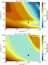 |
Fig. 10 Ratio of column densities of SO2 and SO as function of nH and Vs for G0 = 1 (top) and G0 = 100 (bottom). All other physical parameters are kept constant to the fiducial values and listed on top of the figure. The black cross indicates the position of the fiducial model. |
5 Summary
We have modeled low-velocity (≤ 10 km s−1) nonmagnetized J-type shocks at typical inner envelope densities (105 –108 cm−3) using the Paris-Durham shock code to test SO and SO2 as possible molecular tracers of accretion shocks. The main conclusions of this work are as follows:
In low-velocity (~3 km s−1) shocks, SO can be efficiently formed at intermediate densities (~107 cm−3) through the SH radical reacting with atomic O. Here, SH is formed through S+ reacting primarily with H2CO; though the latter species is a representative of any hydrocarbon.
Both SO and SO2 can be efficiently formed through reactions of atomic S with OH in high-velocity (≳4 km s−1) shocks inlow-intermediate dense environments (≲107 cm−3). The formation of SO and SO2 occurs in the end of the shock, where the abundance of OH is enhanced through photodissociation of earlier formed H2O:
Thermal desorption of SO ice can occur in high-velocity (≳4 km s−1) shocks athigh densities (≳107 cm−3), while thermal desorption of SO2 ice is only relevant at the highest shock velocities (≳10 km s−1) and highest densities (≳108 cm−3);
The chemistry of both SO and SO2 through all formation routes is strongly linked to the strength of the local UV radiation field since the formation of both the OH and SH radicals is dependent on photon processes such as photodissociation and photoionization. In particular, SO2 is only formed in the shock through gas-phase chemistry if the strength of the local UV radiation field is greater or equal to the ISRF;
The composition of infalling material, in both gas-phase species such as atomic O and S and in the ices such as H2S, CH4, SO, and SO2, is highly relevant for the chemistry of SO and SO2 in accretion shocks;
Observations of warm SO and SO2 should be complemented with key species for their formation such as H2S and H2CO. Moreover, the launch of JWST will add additional NIR and MIR accretion shock tracers such as H2, H2O, and [S I] 25 μm.
Our results highlight the key interplay between both physics and chemistry in accretion shocks. The abundances of gas-phase molecules such as SO and SO2 is not solely determined through high-temperature gas-phase chemistry, but also thermal sublimation of ices and photodissociation through UV radiation play an important role. Additional high-angular resolution observations with ALMA are necessary to spatially disentangle the disk from the envelope in embedded systems in order to assess the physical properties of accretion shocks at the disk–envelope interface. Moreover, future facilities such as JWST will provide additional NIR and MIR shock tracers such as H2, OH, and H2O. It is crucial to attain the physical structure of accretion shocks since it determines the chemical composition of material that enters the disk and is eventually incorporated in planets.
Acknowledgements
The authors would like to thank the anonymous referee for their constructive comments on the manuscript. The authors would also like to thank G. Pineau des Forêts for valuable discussions about the project. Astrochemistry in Leiden is supported by the Netherlands Research School for Astronomy (NOVA). M.v.G. and B.T. acknowledge support from the Dutch Research Council (NWO) with project number NWO TOP-1 614.001.751.
Appendix A Updated cooling of NH3
Typically, cooling by NH3 in the optically thin limit is calculated using the empirical relation derived by Le Bourlot et al. (2002). However, this relation does not take into account that the populations get thermalized if the density gets above the critical density. Therefore, the cooling by NH3 is recalculated using the RADEX software (van der Tak et al. 2007). Assuming all emission is optically thin (i.e., low column densities) and emitted through rotational lines, a grid of gas temperatures and H2 densities is set. The full range explored is 5−5000 K and 102 −1012 cm−3, respectively. The linewidth is set to 2 km s−1. The cooling (in erg s−1) for each grid point is calculated by summing over the emission of each spectral line and dividing that by the assumed column density.
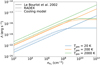 |
Fig. A.1 Cooling by NH3 as function of nH_2 for various Tgas (colors). The empirical relation by Le Bourlot et al. (2002) is shown as the solid lines, the RADEX computations in the dashed line, and the derived cooling function of Eq. (A) in the dotted line. |
Using the cooling grid computed with RADEX, a cooling function, Λ, with Tgas and nH_2 as free parameters can be derived. Minimum χ2 fitting of the grid computed with RADEX was used to calculate Λ, which resulted in,
![Mathematical equation: \begin{align*}\Lambda_{\mathrm{NH}_3}\,{=}\,\Lambda_{\infty} \left(1 - \exp\left[\frac{-n_{\mathrm{H}_2}}{n_{\mathrm{0}}}\right]\right),\end{align*}](/articles/aa/full_html/2021/09/aa41591-21/aa41591-21-eq6.png) (A.1)
(A.1)
with Λ∞ and n0 numerically derived as,
![Mathematical equation: \begin{align*}\Lambda_{\infty} &\,{=}\,2.85\,{\times}\,10^{-15} \left(1 - \exp\left[\frac{-T_{\textrm{gas}}}{81.7}\right] \right){}^4, \\n_{\mathrm{0}} &\,{=}\,8.33\,{\times}\,10^{8} \left(1 - \exp\left[\frac{-T_{\textrm{gas}}}{125} \right] \right).\end{align*}](/articles/aa/full_html/2021/09/aa41591-21/aa41591-21-eq7.png)
Here, Λ∞ is the cooling of NH3 in the LTE limit, whereas n0 is a measure of a critical density above which LTE effects become relevant. Both parameters are dependent on Tgas.
The function in Eq. (A.1) is presented in Fig. A.1 for a few values of Tgas. Overplotted are the RADEX calculations and the empirical relation of Le Bourlot et al. (2002). Indeed, at high densities (≳ 109 cm−3) the latter relation starts overproducing the cooling computed with RADEX by orders of magnitude. However, the updated cooling function represent the cooling by RADEX within a factor of three over the entire temperature and density range. Since densities of ≳ 109 cm−3 are frequently reached in our shock models, the updated cooling function was adopted in the updated version of the shock code.
In high-temperature shocks, significant amounts of NH3 might be producedthrough gas-phase chemistry, enhancing the density and thus the optical depth of the spectral lines. Moreover, the density of NH3 can be increased through ice sublimation in high-density shocks. If the lines of NH3 become optically thick, Eq. (A.1) is no longer valid and cooling tables similar to those of Neufeld & Kaufman (1993) should be calculated for NH3 taking into account opacity effects. This is beyond the scope of this work.
Appendix B Input abundances
The input abundances used in the shock models are presented in Table B.1. The total elemental abundances match those of Flower & Pineau des Forêts (2003). Most of the oxygen, carbon, and sulfur budget is locked up in dust grains and in the ice mantles. The initial abundances of oxygen and nitrogen-bearing ices are equivalent to those presented by Boogert et al. (2015), while the sulfur-bearing ice abundances are matched to those found in both protostellar envelopes and comets (Calmonte et al. 2016; Rubin et al. 2019; Altwegg et al. 2019; Navarro-Almaida et al. 2020). The gas-phase abundances of the key sulfur-bearing molecules, SO, SO2, CS, OCS, and H2S, are taken from van der Tak et al. (2003). All other molecular gas-phase abundances are set equal to those derived on cloud scales by Tafalla et al. (2021). The gas-phase abundance of atomic S in protostellar envelopes is highly uncertain. It is set here at a 10−6 level, which is consistent with the models of Goicoechea & Cuadrado (2021). The effect of initial atomic S abundance on the maximum abundances of SO and SO2 attained in the shock is presented in Sect. 3.2.4.
Dark cloud input abundances
Appendix C Changing the preshock conditions
To test the effect of alteration of infalling dark cloud material in the inner envelope on an accretion shock, various preshock models were calculated. Since the increase in the temperature and protostellar radiation field are negligible in the outer parts of the envelope (e.g., Drozdovskaya et al. 2015), changes in temperature, composition, and ionization balance are most efficient in the inner ~ 1000 AU of the envelope when the material is already approaching the disk and protostar. Given that the infall velocity goes as  , it takes about ~ 100 years to move from 1000 AU to disk scales (~100 AU) for a 0.5 M⊙ star. However, depending on the mass of the protostar and the size of the disk, this preshock timescale tpreshock might range from, for example, ~10 − 104 years. Therefore, the effect of infall time (i.e., tpreshock) on the accretion shock is explored here. The thermal balance is included in the preshock model, but for simplicity the density is assumed to remain constant.
Given that the infalling material is ionized and photodissociated on a timescale of (Heays et al. 2017),
 (C.1)
(C.1)
the ionization balance is fully altered for all tpreshock ≳ 10 years if the strength of the local UV field is G0 ≳ 1. For models with weaker UV fields (G0 = 10−3 − 10−1), the ionization balance is dependent on tpreshock. Moreover, the ice composition may be altered on the photodesorption and adsorption timescales for 0.2 μm grains of (Hollenbach et al. 2009; Godard et al. 2019),

If τionize/disso < τadsorb, any photodesorbed species are dissociated before they can adsorb back on the grain. This increases the abundance of atomic and ionic species.
The abundances of S+, S, SO, SO2, H2S, and s-H2S during a preshock calculation are presented in Fig. C.1 for the fiducial model conditions (see Table 1). Following Eq. (C.1), the ionization balance of S+/S is set after ~ 10 years. However, at longer timescales of ~104 − 105 years, the abundances of both S+ and S increase above the initial abundance of atomic S. On these timescales, H2S ice is photodesorbed (see Eq. (C.2)) and subsequently photodissociated, therefore enhancing the abundance of both atomic S and S+. Since the abundance of H2S is much higher than that of atomic S in the gas phase, already on timescales of 0.1τphotodes the abundance of atomic S is increased with a factor of a few. Meanwhile, the abundance of SO is increased through gas-phase chemistry via Reaction (3), and SO2 is photodissociated into SO and atomic O.
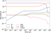 |
Fig. C.1 Abundances of S+, S, SO, SO2, H2S, and s-H2S during a preshock calculation. All physical parameters are kept constant to the fiducial values. |
The effect of the length of the preshock model on the maximum abundances of SO in the subsequent accretion shock is presented in Fig. C.2. Up to tpreshock ≲ 1000 years, the maximum abundance reached in the shock is independent of the time over which the preshock model is calculated. In the tpreshock = 10000 years case, photodesorption and subsequent photodissociation of H2S increases the initial atomic S abundance and hence the maximum abundance of SO reached in the shock. For different strengths of the UV radiation field (i.e., different G0), the timescale for photodesorption changes (i.e., Eq. (C.2)). The effect of tpreshock on the final abundances of SO (and SO2) in the shock is thus negligible if tpreshock is less than roughly ~10% of the photodesorption timescale τphotodes, given that τadsorb > τionize/disso.
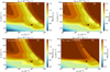 |
Fig. C.2 Maximum abundance reached (in color) of SO in shock models as function of initial nH and Vs after calculating a preshock model for 10 (top left), 100 (top right), 1000 (bottom left), and 10000 (bottom right) years. All other physical parameters are kept constant to the fiducial values and listed on top of the figure. The black cross indicates the position of the fiducial model. The dashed black line shows the ice line, i.e., where 50% of the ice is thermally desorbed into the gas in the shock. |
Appendix D Abundance grids
D.1 H2S, H2O, SiO, and CH3OH for G0 = 1
In Fig. D.1, the maximum abundance for H2S, H2O, SiO, and CH3OH are presented as function of initial nH and Vs. All other parameters are set to their fiducial value (e.g., G0 = 1).
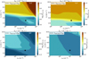 |
Fig. D.1 Similar figure as Fig. 4, but now for H2S (top left), H2O (top right), SiO (bottom left), and CH3OH (bottom right). All other physical parameters are kept constant to the fiducial values and listed on top of the figure. The black cross indicates the position of the fiducial model. The dashed black line shows the ice line, i.e., where 50% of the ice is thermally desorbed into the gas in the shock. |
D.2 SO and SO2 for various G0
In Figs. D.2 and D.3, the maximum abundance for respectively SO and SO2 are presented as function of initial nH and Vs for various strengths of th UV radiation field (i.e., G0 = 10−3 − 102).
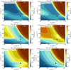 |
Fig. D.2 Maximum abundance reached (in color) of SO in shock models as function of initial nH and Vs for G0 = 10−3 (top left), G0 = 10−2 (top right), G0 = 0.1 (middle left), G0 = 1 (middle right), G0 = 10 (bottom left), and G0 = 100 (bottom right). The black cross indicates the position of the fiducial model. The dashed black line shows the ice line, i.e., where 50% of the ice is thermally desorbed into the gas in the shock. |
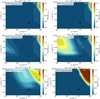 |
Fig. D.3 Maximum abundance reached (in color) of SO2 in shock models as function of initial nH and Vs for G0 = 10−3 (top left), G0 = 10−2 (top right), G0 = 0.1 (middle left), G0 = 1 (middle right), G0 = 10 (bottom left), and G0 = 100 (bottom right). The black cross indicates the position of the fiducial model. The dashed black line shows the ice line, i.e., where 50% of the ice is thermally desorbed into the gas in the shock. |
Appendix E Higher magnetized environments
The focus of this paper is on nonmagnetized J-type shocks. However, in reality magnetic fields are present in protostellar envelopes where observations hint at intermediate or strong magnetic field strengths (i.e., ~0.1 − 1 mG; Hull et al. 2017). The structure of shocks depends strongly on the strength of the magnetic field. In weakly magnetized regions, the emerging shock will remain a magnetized J-type shock with a similar structure to nonmagnetized J-type shocks. However, in higher magnetized environments, the ions and electrons can decouple from the neutral species through the Lorentz force. While slowing down through the Lorentz force, the ions exert a drag force on the neutral fluid. Both fluids slow down and compress, resulting in an increase in the temperature and the emergence of a C-type (strong magnetic field strength) and CJ-type (intermediate magnetic field strength) shocks (Draine 1980; Flower & Pineau des Forêts 2003; Godard et al. 2019). Below, the results of C and CJ-type accretion shocks are shortly discussed, where in both cases a preshock model was calculated over a timescale tpreshock = 100 years (see Appendix C for details).
E.1 C-type shocks
In interstellar C-shocks, the mass of the ionized fluid is dominated by small dust grains (which couple well to ions) and ionized PAHs (e.g., Godard et al. 2019). However, since dust grows to larger grains (here assumed at 0.2 μm) in protostellar evelopes, it will likely be better coupled to the neutral fluid (Guillet et al. 2007, 2020). Moreover, PAHs are lacking in the gas, likely frozen out onto dust grains (Geers et al. 2009). Hence, the mass of the ion fluid exerting a drag force on the neutrals is determined solely by small ions such as S+, C+, HCO+, and N2 H+. Having more small ions (e.g., due to a stronger UV radiation field) therefore strongly affects the structure of the C-type shock.
Since the decoupling between ions and neutrals is very slow, the length of C-type shocks is on envelope scales (i.e., ≳1000 AU) for most of the parameter space considered (see Table 1). Only for high velocity (> 8 km s−1) C-shocks at high densities (> 107 cm−3), the total length of the shock is on disk scales of <100 AU. For such shocks, the abundance of SO is slightly increased through gas-phase chemistry following the green route of Fig. 5, while the abundance of SO2 is not increased in these C-type shocks.
Contrary to J-type shocks, an increased PAHs abundance also affects the physical structure of a C-type shock as ionized PAHs carry most of the mass of the ion fluid if dust grains are assumed to be coupled to the neutrals (Flower & Pineau des Forêts 2003). A higher abundance of PAHs results in a stronger decoupling between ions and neutrals and consequently a decrease in the shock length. Hence, in a larger part of the parameter space, C-type shocks on disk scales (<100 AU) are produced. However, given the lack of PAH emission from Class 0 and I sources (Geers et al. 2009), a high PAH abundance is not realistic.
In reality, any small grains that are present in protostellar envelopes could be coupled to the ions (Guillet et al. 2007; Godard et al. 2019). In turn, this also results in a larger fraction of the parameter space having a shock length of < 100 AU. However, the full treatment ofgrain dynamics in C-type shocks would have to include a separate fluid for each grain size (Ciolek & Roberge 2002; Guillet et al. 2007) with grain-grain interactions such as vaporization, shattering, and coagulation (Guillet et al. 2009, 2011). This is beyond the scope of this work.
E.2 CJ-type shocks
With decreasing magnetic field strength, the decoupling between ions and neutrals becomes weaker. The motion of the neutral velocity is no longer completely dominated by the ion-neutral drag, but also by the viscous stresses and thermal pressure gradient (Godard et al. 2019). The resulting CJ-shock structure is presented in left part of Fig. E.1 for B ~ 160 μG. All other parameters are kept at their fiducial value (see Table 1). Initially, the drag of the ions slows down the neutrals, increasing the gas temperature to ~50 K. However, here the viscous stresses and thermal pressure take over, resulting in a jump in temperature and density as the neutral fluid jumps across the sonic point (Godard et al. 2019). Afterwards, the ions keep exerting a small drag force on the neutrals until the fluids recouple at about ~80 AU. Since the heating induced by this drag is lower than the cooling of the gas, the shock gradually cools down. The abundances of SO and SO2 do show an increase in the CJ-shock, see right panel of Fig. E.1. Here, SO is predominantly formed through Reaction (2) with SH coming from the green route of Fig. 5.
Given that the strength of the magnetic field on inner envelope scales might be high enough to create CJ-type shocks (Hull et al. 2017), these type of shocks are very relevant. However, in order to compute CJ-type shocks over the entire parameter space considered in this paper, the Paris-Durham shock code has to be tweaked to our specific parameter space. This is beyond the scope of this work. Nevertheless, as shown in Fig. E.1, the chemical formation routes of Fig. 5 are still valid for CJ-type shocks sincesimilar physical conditions are attained.
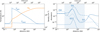 |
Fig. E.1 Same as Fig. 2, but for a CJ-type shock with B ~ 160 μG. All other parameters are kept at their fiducial value (see Table 1). In the right panel, the region where Tgas >50 K is indicated with the shaded blue region. |
References
- Aikawa, Y., Umebayashi, T., Nakano, T., & Miyama, S. M. 1999, ApJ, 519, 705 [NASA ADS] [CrossRef] [Google Scholar]
- Altwegg, K., Balsiger, H., & Fuselier, S. A. 2019, ARA&A, 57, 113 [NASA ADS] [CrossRef] [Google Scholar]
- Aota, T., Inoue, T., & Aikawa, Y. 2015, ApJ, 799, 141 [NASA ADS] [CrossRef] [Google Scholar]
- Artur de la Villarmois, E., Jørgensen, J. K., Kristensen, L. E., et al. 2019, A&A, 626, A71 [NASA ADS] [CrossRef] [EDP Sciences] [Google Scholar]
- Banzatti, A., Pascucci, I., Edwards, S., et al. 2019, ApJ, 870, 76 [NASA ADS] [CrossRef] [Google Scholar]
- Benz, A. O., Bruderer, S., van Dishoeck, E. F., et al. 2016, A&A, 590, A105 [NASA ADS] [CrossRef] [EDP Sciences] [Google Scholar]
- Bjerkeli, P., Ramsey, J. P., Harsono, D., et al. 2019, A&A, 631, A64 [NASA ADS] [CrossRef] [EDP Sciences] [Google Scholar]
- Black, J. H., & van Dishoeck, E. F. 1987, ApJ, 322, 412 [NASA ADS] [CrossRef] [Google Scholar]
- Boogert, A. C. A., Schutte, W. A., Helmich, F. P., Tielens, A. G. G. M., & Wooden, D. H. 1997, A&A, 317, 929 [NASA ADS] [Google Scholar]
- Boogert, A. C. A., Gerakines, P. A., & Whittet, D. C. B. 2015, ARA&A, 53, 541 [Google Scholar]
- Calmonte, U., Altwegg, K., Balsiger, H., et al. 2016, MNRAS, 462, S253 [CrossRef] [Google Scholar]
- Caselli, P., Hartquist, T. W., & Havnes, O. 1997, A&A, 322, 296 [NASA ADS] [Google Scholar]
- Cassen, P., & Moosman, A. 1981, Icarus, 48, 353 [NASA ADS] [CrossRef] [Google Scholar]
- Ciolek, G. E., & Roberge, W. G. 2002, ApJ, 567, 947 [NASA ADS] [CrossRef] [Google Scholar]
- Codella, C., Maury, A. J., Gueth, F., et al. 2014, A&A, 563, L3 [NASA ADS] [CrossRef] [EDP Sciences] [Google Scholar]
- Codella, C., Ceccarelli, C., Bianchi, E., et al. 2020, A&A, 635, A17 [NASA ADS] [CrossRef] [EDP Sciences] [Google Scholar]
- Draine, B. T. 1980, ApJ, 241, 1021 [NASA ADS] [CrossRef] [Google Scholar]
- Draine, B. T.,& Li, A. 2007, ApJ, 657, 810 [NASA ADS] [CrossRef] [Google Scholar]
- Draine, B. T., Roberge, W. G., & Dalgarno, A. 1983, ApJ, 264, 485 [NASA ADS] [CrossRef] [Google Scholar]
- Drozdovskaya,M. N., Walsh, C., Visser, R., Harsono, D., & van Dishoeck, E. F. 2015, MNRAS, 451, 3836 [NASA ADS] [CrossRef] [Google Scholar]
- Drozdovskaya,M. N., van Dishoeck, E. F., Jørgensen, J. K., et al. 2018, MNRAS, 476, 4949 [NASA ADS] [CrossRef] [Google Scholar]
- Drozdovskaya,M. N., van Dishoeck, E. F., Rubin, M., Jørgensen, J. K., & Altwegg, K. 2019, MNRAS, 490, 50 [NASA ADS] [CrossRef] [Google Scholar]
- Flower, D. R., & Pineau des Forêts, G. 2003, MNRAS, 343, 390 [NASA ADS] [CrossRef] [Google Scholar]
- Flower, D. R. & Pineau des Forêts, G. 2010, MNRAS, 406, 1745 [Google Scholar]
- Flower, D. R. & Pineau des Forêts, G. 2015, A&A, 578, A63 [NASA ADS] [CrossRef] [EDP Sciences] [Google Scholar]
- Galametz, M., Maury, A. J., Valdivia, V., et al. 2019, A&A, 632, A5 [NASA ADS] [CrossRef] [EDP Sciences] [Google Scholar]
- Geballe, T. R., Baas, F., Greenberg, J. M., & Schutte, W. 1985, A&A, 146, L6 [NASA ADS] [Google Scholar]
- Geers, V. C., van Dishoeck, E. F., Pontoppidan, K. M., et al. 2009, A&A, 495, 837 [NASA ADS] [CrossRef] [EDP Sciences] [Google Scholar]
- Godard, B., Pineau des Forêts, G., Lesaffre, P., et al. 2019, A&A, 622, A100 [NASA ADS] [CrossRef] [EDP Sciences] [Google Scholar]
- Goicoechea, J. R., & Cuadrado, S. 2021, A&A, 647, L7 [NASA ADS] [CrossRef] [EDP Sciences] [Google Scholar]
- Goicoechea, J. R., Cernicharo, J., Karska, A., et al. 2012, A&A, 548, A77 [NASA ADS] [CrossRef] [EDP Sciences] [Google Scholar]
- Guillet, V., Pineau Des, G., & Jones, A. P. 2007, A&A, 476, 263 [NASA ADS] [CrossRef] [EDP Sciences] [Google Scholar]
- Guillet, V., Jones, A. P., & Pineau des Forêts, G. 2009, A&A, 497, 145 [NASA ADS] [CrossRef] [EDP Sciences] [Google Scholar]
- Guillet, V., Pineau des Forêts, G., & Jones, A. P. 2011, A&A, 527, A123 [NASA ADS] [CrossRef] [EDP Sciences] [Google Scholar]
- Guillet, V., Hennebelle, P., Pineau des Forêts, G., et al. 2020, A&A, 643, A17 [EDP Sciences] [Google Scholar]
- Guilloteau, S., Bachiller, R., Fuente, A., & Lucas, R. 1992, A&A, 265, L49 [NASA ADS] [Google Scholar]
- Gusdorf, A., Cabrit, S., Flower, D. R., & Pineau des Forêts, G. 2008a, A&A, 482, 809 [NASA ADS] [CrossRef] [EDP Sciences] [Google Scholar]
- Gusdorf, A., Pineau des Forêts, G., Cabrit, S., & Flower, D. R. 2008b, A&A, 490, 695 [NASA ADS] [CrossRef] [EDP Sciences] [Google Scholar]
- Harsono, D., van Dishoeck, E. F., Bruderer, S., Li, Z. Y., & Jørgensen, J. K. 2015, A&A, 577, A22 [NASA ADS] [CrossRef] [EDP Sciences] [Google Scholar]
- Harsono, D., Bjerkeli, P., van der Wiel, M. H. D., et al. 2018, Nat. Astron., 2, 646 [NASA ADS] [CrossRef] [Google Scholar]
- Harsono, D., van der Wiel, M. H. D., Bjerkeli, P., et al. 2021, A&A, 646, A72 [NASA ADS] [CrossRef] [EDP Sciences] [Google Scholar]
- Hartquist, T. W., Dalgarno, A., & Oppenheimer, M. 1980, ApJ, 236, 182 [NASA ADS] [CrossRef] [Google Scholar]
- Heays, A. N., Bosman, A. D., & van Dishoeck, E. F. 2017, A&A, 602, A105 [NASA ADS] [CrossRef] [EDP Sciences] [Google Scholar]
- Herczeg, G. J., Karska, A., Bruderer, S., et al. 2012, A&A, 540, A84 [NASA ADS] [CrossRef] [EDP Sciences] [Google Scholar]
- Holdship, J., Viti, S., Jimenez-Serra, I., et al. 2016, MNRAS, 463, 802 [NASA ADS] [CrossRef] [Google Scholar]
- Hollenbach, D., Kaufman, M. J., Bergin, E. A., & Melnick, G. J. 2009, ApJ, 690, 1497 [CrossRef] [Google Scholar]
- Hull, C. L. H., Mocz, P., Burkhart, B., et al. 2017, ApJ, 842, L9 [NASA ADS] [CrossRef] [Google Scholar]
- Jiménez-Escobar, A., & Muñoz Caro, G. M. 2011, A&A, 536, A91 [NASA ADS] [CrossRef] [EDP Sciences] [Google Scholar]
- Karska, A., Kaufman, M. J., Kristensen, L. E., et al. 2018, ApJS, 235, 30 [NASA ADS] [CrossRef] [Google Scholar]
- Kristensen, L. E., van Dishoeck, E. F., Bergin, E. A., et al. 2012, A&A, 542, A8 [NASA ADS] [CrossRef] [EDP Sciences] [Google Scholar]
- Lahuis, F., van Dishoeck, E. F., Jørgensen, J. K., Blake, G. A., & Evans, N. J. 2010, A&A, 519, A3 [NASA ADS] [CrossRef] [EDP Sciences] [Google Scholar]
- Le Bourlot J., Pineau des Forêts, G., Flower, D. R., & Cabrit, S. 2002, MNRAS, 332, 985 [NASA ADS] [CrossRef] [Google Scholar]
- Lee, C.-F., Li, Z.-Y., Codella, C., et al. 2018, ApJ, 856, 14 [NASA ADS] [CrossRef] [Google Scholar]
- Lesaffre, P., Pineau des Forêts, G., Godard, B., et al. 2013, A&A, 550, A106 [NASA ADS] [CrossRef] [EDP Sciences] [Google Scholar]
- Li, Z.-Y., Krasnopolsky, R., & Shang, H. 2013, ApJ, 774, 82 [NASA ADS] [CrossRef] [Google Scholar]
- Manara, C. F., Morbidelli, A., & Guillot, T. 2018, A&A, 618, A3 [NASA ADS] [CrossRef] [EDP Sciences] [Google Scholar]
- Mathis, J. S., Rumpl, W., & Nordsieck, K. H. 1977, ApJ, 217, 425 [NASA ADS] [CrossRef] [Google Scholar]
- Mathis, J. S., Mezger, P. G., & Panagia, N. 1983, A&A, 500, 259 [NASA ADS] [Google Scholar]
- McCaughrean,M. J., Rayner, J. T., & Zinnecker, H. 1994, ApJ, 436, L189 [Google Scholar]
- Miotello, A., Testi, L., Lodato, G., et al. 2014, A&A, 567, A32 [NASA ADS] [CrossRef] [EDP Sciences] [Google Scholar]
- Miura, H., Yamamoto, T., Nomura, H., et al. 2017, ApJ, 839, 47 [NASA ADS] [CrossRef] [Google Scholar]
- Mumma, M. J., & Charnley, S. B. 2011, ARA&A, 49, 471 [NASA ADS] [CrossRef] [Google Scholar]
- Murillo, N. M., Lai, S.-P., Bruderer, S., Harsono, D., & van Dishoeck, E. F. 2013, A&A, 560, A103 [NASA ADS] [CrossRef] [EDP Sciences] [Google Scholar]
- Navarro-Almaida, D., Le Gal, R., Fuente, A., et al. 2020, A&A, 637, A39 [CrossRef] [EDP Sciences] [Google Scholar]
- Neufeld, D. A., & Hollenbach, D. J. 1994, ApJ, 428, 170 [NASA ADS] [CrossRef] [Google Scholar]
- Neufeld, D. A., & Kaufman, M. J. 1993, ApJ, 418, 263 [NASA ADS] [CrossRef] [Google Scholar]
- Neufeld, D. A., Nisini, B., Giannini, T., et al. 2009, ApJ, 706, 170 [NASA ADS] [CrossRef] [Google Scholar]
- Nisini, B., Santangelo, G., Antoniucci, S., et al. 2013, A&A, 549, A16 [NASA ADS] [CrossRef] [EDP Sciences] [Google Scholar]
- Nisini, B., Santangelo, G., Giannini, T., et al. 2015, ApJ, 801, 121 [NASA ADS] [CrossRef] [EDP Sciences] [Google Scholar]
- Owen, T., Bar-Nun, A., & Kleinfeld, I. 1992, Nature, 358, 43 [NASA ADS] [CrossRef] [Google Scholar]
- Oya, Y., López-Sepulcre, A., Sakai, N., et al. 2019, ApJ, 881, 112 [Google Scholar]
- Palumbo, M. E., Tielens, A. G. G. M., & Tokunaga, A. T. 1995, ApJ, 449, 674 [NASA ADS] [CrossRef] [Google Scholar]
- Penteado, E. M., Walsh, C., & Cuppen, H. M. 2017, ApJ, 844, 71 [NASA ADS] [CrossRef] [Google Scholar]
- Podio, L., Eislöffel, J., Melnikov, S., Hodapp, K. W., & Bacciotti, F. 2011, A&A, 527, A13 [NASA ADS] [CrossRef] [EDP Sciences] [Google Scholar]
- Prasad, S. S., & Huntress, W. T., J. 1980, ApJS, 43, 1 [NASA ADS] [CrossRef] [Google Scholar]
- Rivière-Marichalar, P., Merín, B., Kamp, I., Eiroa, C., & Montesinos, B. 2016, A&A, 594, A59 [NASA ADS] [CrossRef] [EDP Sciences] [Google Scholar]
- Rubin, M., Altwegg, K., Balsiger, H., et al. 2019, MNRAS, 489, 594 [CrossRef] [Google Scholar]
- Sakai, N., Sakai, T., Hirota, T., et al. 2014, Nature, 507, 78 [NASA ADS] [CrossRef] [Google Scholar]
- Sakai, N., Oya, Y., Higuchi, A. E., et al. 2017, MNRAS, 467, L76 [NASA ADS] [Google Scholar]
- Schilke, P., Walmsley, C. M., Pineau des Forêts, G., & Flower, D. R. 1997, A&A, 321, 293 [Google Scholar]
- Suutarinen, A. N., Kristensen, L. E., Mottram, J. C., Fraser, H. J., & van Dishoeck, E. F. 2014, MNRAS, 440, 1844 [NASA ADS] [CrossRef] [Google Scholar]
- Tabone, B., Cabrit, S., Bianchi, E., et al. 2017, A&A, 607, L6 [NASA ADS] [CrossRef] [EDP Sciences] [Google Scholar]
- Tabone, B., Godard, B., Pineau des Forêts, G., Cabrit, S., & van Dishoeck, E. F. 2020, A&A, 636, A60 [CrossRef] [EDP Sciences] [Google Scholar]
- Tabone, B., van Hemert, M. C., van Dishoeck, E. F., & Black, J. H. 2021, A&A, 650, A192 [NASA ADS] [CrossRef] [EDP Sciences] [Google Scholar]
- Tafalla, M., Usero, A., & Hacar, A. 2021, A&A, 646, A97 [NASA ADS] [CrossRef] [EDP Sciences] [Google Scholar]
- Taquet, V., Codella, C., De Simone, M., et al. 2020, A&A, 637, A63 [CrossRef] [EDP Sciences] [Google Scholar]
- Tobin, J. J., Hartmann, L., Chiang, H.-F., et al. 2012, Nature, 492, 83 [NASA ADS] [CrossRef] [PubMed] [Google Scholar]
- Tychoniec, Ł., Hull, C. L. H., Kristensen, L. E., et al. 2019, A&A, 632, A101 [NASA ADS] [CrossRef] [EDP Sciences] [Google Scholar]
- Tychoniec, Ł., Manara, C. F., Rosotti, G. P., et al. 2020, A&A, 640, A19 [CrossRef] [EDP Sciences] [Google Scholar]
- Tychoniec, Ł., van Dishoeck, E. F., van ’t Hoff, M. L. R., et al. 2021, A&A, in press https://doi.org/10.1051/0004-6361/202140692 [Google Scholar]
- van der Tak, F. F. S., Boonman, A. M. S., Braakman, R., & van Dishoeck, E. F. 2003, A&A, 412, 133 [NASA ADS] [CrossRef] [EDP Sciences] [Google Scholar]
- van der Tak, F. F. S., Black, J. H., Schöier, F. L., Jansen, D. J., & van Dishoeck, E. F. 2007, A&A, 468, 627 [NASA ADS] [CrossRef] [EDP Sciences] [Google Scholar]
- van Dishoeck, E. F., Kristensen, L. E., Mottram, J. C., et al. 2021, A&A, 648, A24 [CrossRef] [EDP Sciences] [Google Scholar]
- van Kempen, T. A., van Dishoeck, E. F., Güsten, R., et al. 2009, A&A, 501, 633 [NASA ADS] [CrossRef] [EDP Sciences] [Google Scholar]
- van ’t Hoff, M. L. R., Tobin, J. J., Harsono, D., & van Dishoeck, E. F. 2018, A&A, 615, A83 [NASA ADS] [CrossRef] [EDP Sciences] [Google Scholar]
- Vidal, T. H. G., Loison, J.-C., Jaziri, A. Y., et al. 2017, MNRAS, 469, 435 [Google Scholar]
- Visser, R., & Dullemond, C. P. 2010, A&A, 519, A28 [NASA ADS] [CrossRef] [EDP Sciences] [Google Scholar]
- Visser, R., van Dishoeck, E. F., Doty, S. D., & Dullemond, C. P. 2009, A&A, 495, 881 [NASA ADS] [CrossRef] [EDP Sciences] [Google Scholar]
- Visser, R., Kristensen, L. E., Bruderer, S., et al. 2012, A&A, 537, A55 [NASA ADS] [CrossRef] [EDP Sciences] [Google Scholar]
- Y"i"ld"i"z, U. A., Kristensen, L. E., van Dishoeck, E. F., et al. 2012, A&A, 542, A86 [NASA ADS] [CrossRef] [EDP Sciences] [Google Scholar]
- Zasowski, G., Kemper, F., Watson, D. M., et al. 2009, ApJ, 694, 459 [NASA ADS] [CrossRef] [Google Scholar]
All Tables
All Figures
|
Fig. 1 Physical structure of a protostellar envelope. Starting with dark cloud conditions, an accretion shock model is calculated. The shock profile in the bottom panel is shown on a logarithmic scale with the yellow region indicating the shocked region. |
| In the text | |
|
Fig. 2 Left: temperature and density structure in the fiducial J-type shock. The shock starts at 0 AU and ends at about 5 AU. The dust temperature does not increase enough for thermal sublimation of SO and SO2. Right: abundance profiles of SO (solid) and SO2 (dashed) and the key species for gas-phase formation of these species: SH (dot-dashed) and OH (dotted). The region where Tgas >50 K is indicated with the shaded blue region. |
| In the text | |
|
Fig. 3 Maximum dust temperature reached (in color) in shock models as function of initial nH and Vs. All other physical parameters are kept constant to the fiducial values and listed on top of the figure. The black cross indicates the position of the fiducial model. |
| In the text | |
|
Fig. 4 Maximum abundance reached (in color) of SO (left) and SO2 (right) in shock models as function of initial nH and Vs. All other physical parameters are kept constant to the fiducial values and listed on top of the figure. The black cross indicates the position of the fiducial model. The dashed black line shows the ice line, i.e., where 50% of the ice is thermally desorbed into the gas in the shock. |
| In the text | |
|
Fig. 5 Chemical reactions leading to the formation of gas-phase SO and SO2. Species denoted as s-X are located in the ice mantles of dust grains. Reverse reactions are not shown for clarity. Red arrows denote chemical reactions with the annotated species, yellow arrows photodissociation reactions, and blue arrows ice desorption via either thermal or nonthermal mechanisms. Relevant chemical pathways are highlighted with a colored background. |
| In the text | |
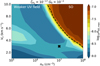 |
Fig. 6 Similar figure as Fig. 4, but now for SO in shocks with a weaker UV field (G0 = 10−2). |
| In the text | |
|
Fig. 7 Maximum abundance reached (in color) of SO (left) and SO2 (right) in shock models as function of initial nH and Vs for an initial gas-phase atomic S abundance of 10−8 (top row) and 10−5 (bottom row). All other physical parameters are kept constant to the fiducial values and listed on top of the figure. The black cross indicates the position of the fiducial model. The dashed black line shows the ice line, i.e., where 50% of the ice is thermally desorbed into the gas in the shock. |
| In the text | |
|
Fig. 8 Abundance profile of SO (solid) and SO2 (dashed) for the fiducial model (blue) with a PAH abundance of 10−8 using a grainsize of 0.2 μm. Overplotted are the same model using a typical ISM grain size of 0.03 μm (orange) anda model with a PAH abundance of 10−6 (green). All other parameters are kept at their fiducial value (see Table 1). |
| In the text | |
|
Fig. 9 Rotational diagram of H2 created from the fiducial shock model. The levels of different vibrational states are indicated with different symbols and colors. Only the pure rotational levels with Eu ∕kB≲ 6000 K are collisionally populated. The fit to the pure rotational levels is shown in gray line with the derived rotational temperature annotated. |
| In the text | |
|
Fig. 10 Ratio of column densities of SO2 and SO as function of nH and Vs for G0 = 1 (top) and G0 = 100 (bottom). All other physical parameters are kept constant to the fiducial values and listed on top of the figure. The black cross indicates the position of the fiducial model. |
| In the text | |
|
Fig. A.1 Cooling by NH3 as function of nH_2 for various Tgas (colors). The empirical relation by Le Bourlot et al. (2002) is shown as the solid lines, the RADEX computations in the dashed line, and the derived cooling function of Eq. (A) in the dotted line. |
| In the text | |
|
Fig. C.1 Abundances of S+, S, SO, SO2, H2S, and s-H2S during a preshock calculation. All physical parameters are kept constant to the fiducial values. |
| In the text | |
|
Fig. C.2 Maximum abundance reached (in color) of SO in shock models as function of initial nH and Vs after calculating a preshock model for 10 (top left), 100 (top right), 1000 (bottom left), and 10000 (bottom right) years. All other physical parameters are kept constant to the fiducial values and listed on top of the figure. The black cross indicates the position of the fiducial model. The dashed black line shows the ice line, i.e., where 50% of the ice is thermally desorbed into the gas in the shock. |
| In the text | |
|
Fig. D.1 Similar figure as Fig. 4, but now for H2S (top left), H2O (top right), SiO (bottom left), and CH3OH (bottom right). All other physical parameters are kept constant to the fiducial values and listed on top of the figure. The black cross indicates the position of the fiducial model. The dashed black line shows the ice line, i.e., where 50% of the ice is thermally desorbed into the gas in the shock. |
| In the text | |
|
Fig. D.2 Maximum abundance reached (in color) of SO in shock models as function of initial nH and Vs for G0 = 10−3 (top left), G0 = 10−2 (top right), G0 = 0.1 (middle left), G0 = 1 (middle right), G0 = 10 (bottom left), and G0 = 100 (bottom right). The black cross indicates the position of the fiducial model. The dashed black line shows the ice line, i.e., where 50% of the ice is thermally desorbed into the gas in the shock. |
| In the text | |
|
Fig. D.3 Maximum abundance reached (in color) of SO2 in shock models as function of initial nH and Vs for G0 = 10−3 (top left), G0 = 10−2 (top right), G0 = 0.1 (middle left), G0 = 1 (middle right), G0 = 10 (bottom left), and G0 = 100 (bottom right). The black cross indicates the position of the fiducial model. The dashed black line shows the ice line, i.e., where 50% of the ice is thermally desorbed into the gas in the shock. |
| In the text | |
|
Fig. E.1 Same as Fig. 2, but for a CJ-type shock with B ~ 160 μG. All other parameters are kept at their fiducial value (see Table 1). In the right panel, the region where Tgas >50 K is indicated with the shaded blue region. |
| In the text | |
Current usage metrics show cumulative count of Article Views (full-text article views including HTML views, PDF and ePub downloads, according to the available data) and Abstracts Views on Vision4Press platform.
Data correspond to usage on the plateform after 2015. The current usage metrics is available 48-96 hours after online publication and is updated daily on week days.
Initial download of the metrics may take a while.