| Issue |
A&A
Volume 653, September 2021
|
|
|---|---|---|
| Article Number | A49 | |
| Number of page(s) | 27 | |
| Section | Stellar structure and evolution | |
| DOI | https://doi.org/10.1051/0004-6361/202141031 | |
| Published online | 07 September 2021 | |
The CARMENES search for exoplanets around M dwarfs
Spectroscopic orbits of nine M-dwarf multiple systems, including two triples, two brown dwarf candidates, and one close M-dwarf–white dwarf binary
1
Institut de Ciències de l’Espai (ICE, CSIC), Campus UAB, c/ Can Magrans s/n, 08193 Bellaterra, Barcelona, Spain
e-mail: This email address is being protected from spambots. You need JavaScript enabled to view it.
2
Institut d’Estudis Espacials de Catalunya (IEEC), c/ Gran Capità 2–4, 08034 Barcelona, Spain
3
Instituto de Astrofísica de Canarias, Vía Láctea s/n, 38205 La Laguna, Tenerife, Spain
4
Departamento de Astrofísica, Universidad de La Laguna, 38026 La Laguna, Tenerife, Spain
5
Landessternwarte, Zentrum für Astronomie der Universität Heidelberg, Königstuhl 12, 69117 Heidelberg, Germany
6
Institut für Astrophysik, Georg-August-Universität, Friedrich-Hund-Platz 1, 37077 Göttingen, Germany
7
Centro de Astrobiología (CSIC-INTA), ESAC, Camino Bajo del Castillo s/n, 28692 Villanueva de la Cañada, Madrid, Spain
8
Instituto de Astrofísica de Andalucía (IAA-CSIC), Glorieta de la Astronomía s/n, 18008 Granada, Spain
9
Spanish Virtual Observatory, Spain
10
Centro Astronónomico Hispano Alemán, Observatorio de Calar Alto, Sierra de los Filabres, 04550 Gérgal, Spain
11
Thüringer Landesstenwarte Tautenburg, Sternwarte 5, 07778 Tautenburg, Germany
12
Max Planck Institute for Solar System Research, Justus-von-Liebig-Weg 3, 37077 Göttingen, Germany
13
Max-Planck-Institut für Astronomie, Königstuhl 17, 69117 Heidelberg, Germany
14
Departamento de Física de la Tierra y Astrofísica and IPARCOS-UCM (Instituto de Física de Partículas y del Cosmos de la UCM), Facultad de Ciencias Físicas, Universidad Complutense de Madrid, 28040 Madrid, Spain
15
Department of Physics, University of Warwick, Gibbet Hill Road, Coventry CV4 7AL, UK
16
Hamburger Sternwarte, Gojenbergsweg 112, 21029 Hamburg, Germany
17
Department of Physics, Ariel University, Ariel 40700, Israel
Received:
9
April
2021
Accepted:
29
May
2021
Abstract
Context. M dwarfs are ideal targets for the search of Earth-size planets in the habitable zone using the radial velocity method, and are attracting the attention of many ongoing surveys. One of the expected results of these surveys is that new multiple-star systems have also been found. This is the case also for the CARMENES survey, thanks to which nine new double-line spectroscopic binary systems have already been announced.
Aims. Throughout the five years of the survey the accumulation of new observations has resulted in the detection of several new multiple-stellar systems with long periods and low radial-velocity amplitudes. Here we newly characterise the spectroscopic orbits and constrain the masses of eight systems and update the properties of a system that we had reported earlier.
Methods. We derived the radial velocities of the stars using two-dimensional cross-correlation techniques and template matching. The measurements were modelled to determine the orbital parameters of the systems. We combined CARMENES spectroscopic observations with archival high-resolution spectra from other instruments to increase the time span of the observations and improve our analysis. When available, we also added archival photometric, astrometric, and adaptive optics imaging data to constrain the rotation periods and absolute masses of the components.
Results. We determined the spectroscopic orbits of nine multiple systems, eight of which are presented for the first time. The sample is composed of five single-line binaries, two double-line binaries, and two triple-line spectroscopic triple systems. The companions of two of the single-line binaries, GJ 3626 and GJ 912, have minimum masses below the stellar boundary, and thus could be brown dwarfs. We found a new white dwarf in a close binary orbit around the M star GJ 207.1, located at a distance of 15.79 pc. From a global fit to radial velocities and astrometric measurements, we were able to determine the absolute masses of the components of GJ 282 C, which is one of the youngest systems with measured dynamical masses.
Key words: stars: low-mass / brown dwarfs / white dwarfs / binaries: spectroscopic / astrometry
© ESO 2021
1. Introduction
M dwarfs constitute the majority of stars in the Galaxy, in both number and mass (Gizis et al. 2002), and comprise almost 75% of the stars in the solar neighbourhood (Henry et al. 2006). Over 40% of M dwarfs are found in multiple systems (Cortés-Contreras et al. 2017; Winters et al. 2019), making them a key ingredient to our understanding of the stellar population as a whole. Statistical studies of their properties, such as the distribution of mass ratio and orbital elements, provide crucial tests for star formation theories and evolutionary models (see e.g. Tohline 2002; Duchêne & Kraus 2013). Depending on their orbital architecture, dynamical analyses of binary systems can yield individual masses and radii with a precision of a few percent independently from calibrations and stellar models (Andersen 1991; Torres et al. 2010; Southworth 2015). These masses and radii are of key importance for tests of stellar models, and to determine empirical calibrations that can be applied to derive the fundamental properties of single stars (Baraffe et al. 2015; Benedict et al. 2016; Mann et al. 2019; Schweitzer et al. 2019). The determination of precise masses and radii is particularly relevant for M-dwarf binaries, which show discrepancies with stellar model predictions (Morales et al. 2010; Tal-Or et al. 2013; Feiden & Chaboyer 2014).
Apart from their interest as a major galactic population, M dwarfs have also gained significant attention in the field of exoplanets. A number of surveys searching for rocky habitable planets using radial velocities (RVs) and the transit technique focus on M-dwarf stars, in which Earth-size planetary companions are common (Dressing & Charbonneau 2013). Moreover, compared to Sun-like stars, M dwarfs have the critical advantages of having lower mass and closer habitable zones (Kasting et al. 1993; Kopparapu et al. 2013). This means that potentially habitable planets would induce larger RV signals and would be easier to detect than around earlier-type stars. A benefit of these exoplanet surveys is the large number of new stellar multiple systems that have also been discovered (e.g. Kirk et al. 2016; Baroch et al. 2018; Sperauskas et al. 2019).
The CARMENES survey (Quirrenbach et al. 2018, 2020) is an example of one such exoplanet survey. It has observed more than 300 M-dwarf stars searching for exoplanets in their habitable zones, and has already discovered ∼30 planets (e.g. Ribas et al. 2018; Morales et al. 2019; Zechmeister et al. 2019; Trifonov et al. 2021). Furthermore, CARMENES has also revealed the binary nature of nine new M-dwarf systems for which orbital elements were computed by Baroch et al. (2018). We announce here eight new multiple systems that were not observed or could not be resolved by Baroch et al. (2018), and also use new observations to determine the orbital parameters of the very long-period SB2 system UU UMi, which was already analysed by Baroch et al. (2018). These systems include two triple-line spectroscopic triple systems (ST3), two double-line spectroscopic binaries (SB2), and five single-line spectroscopic binaries (SB1), two of which have companions with masses compatible with them being substellar, and another with a white dwarf star in a close-in orbit. In Sect. 2 we list the studied stars and describe the observations used in our analysis, including available data in public archives. Section 3 explains the method used to measure the RVs from observations and to obtain the orbital parameters and rotation periods. In Sect. 4 we present the results for each system. Finally, in Sect. 5 we discuss the peculiarities of some of the systems and conclude our work.
2. Sample selection and data
2.1. Spectroscopic data
The CARMENES survey is spectroscopically monitoring over 300 M-dwarf stars in a search for exoplanets. The visual channel of the CARMENES spectrograph covers a wavelength range from 0.52 μm to 0.96 μm dispersed across 61 échelle orders, with a measured resolving power of R = 94 600. A more detailed description of the CARMENES instrument was provided by Quirrenbach et al. (2014, 2016). Reduction of raw spectra is automatically performed by the caracal (CARMENES Reduction And Calibration, Caballero et al. 2016) pipeline, which corrects for bias, flat-field, and cosmic rays, and extracts one-dimensional wavelength-calibrated spectra. High-precision RVs are routinely computed with the serval pipeline, which also computes activity indicators such as the chromatic index (CRX) and the differential line width (dLW), along with other spectroscopic indices (Zechmeister et al. 2018). A simple search for stars showing RV excursions greater than ∼0.5 km s−1 revealed eight new multiple stellar system candidates, in addition to the nine SB2s already announced by Baroch et al. (2018). A total of 269 high-resolution spectra of these stars were obtained from January 2016 to December 2020 with the visual channel of the CARMENES spectrograph, including the UU UMi spectra already studied by Baroch et al. (2018). Table 1 lists the main properties of the stars studied here. It includes their common names and CARMENES identifiers, their equatorial coordinates, distances, and proper motions, their G-, V-, and J-band magnitudes, and different spectroscopic indicators, all computed assuming non-binarity, and therefore subject to some bias. It also lists the renormalised unit weight error (RUWE) from Gaia, which is an indicator of the goodness of the fit of the astrometric observations. A RUWE ≳1.4 may indicate that the source is not single. The astrometric properties of all systems are from the Gaia Early Data Release 3 (Gaia Collaboration 2021).
Astrometric, photometric, and spectroscopic properties of the nine systems studied in this work.
We also collected additional high-resolution spectroscopic observations from public archives in order to complement our observations for long-period systems. We found a total of 104 additional observations, 60 taken with the HARPS spectrograph at La Silla Observatory (Mayor et al. 2003), 37 with the FEROS spectrograph also at La Silla Observatory (Kaufer et al. 1999), 6 spectra with the UVES spectrograph at Paranal Observatory (Dekker et al. 2000), and, 1 with the CAFE spectrograph at Calar Alto Observatory (Aceituno et al. 2013), obtained by Jeffers et al. (2018) as part of the characterisation of the CARMENES input catalogue of stars. In total we gathered 373 high-resolution spectra for the nine systems studied in this work, increasing the time span of the observations to up to 15 years for some systems. A summary of the number of observations available from each instrument is given in Table 2.
Number of spectroscopic observations and their time spans, and photometric epochs after and before (in parentheses) filtering and binning.
2.2. Photometric data
In order to check for possible eclipses or rotational variability, we collected photometric time series from public archives of surveys such as TESS (Ricker et al. 2015), ASAS (Pojmanski 1997), NSVS (Woźniak et al. 2004), and MEarth (Berta et al. 2012), and from not-yet public data from SWASP (Pollacco et al. 2006). We refer to Díez Alonso et al. (2019) for details on these surveys. Within the context of the CARMENES spectroscopic survey, photometric follow-up was triggered from ground-based observatories for some interesting candidates. In particular, we collected R-band photometric data of GJ 207.1 at the Montsec Astronomical Observatory1 using the Telescopi Joan Oró (TJO) and the MEIA2 instrument. TJO is a fully robotic 0.8 m Ritchey-Chrétien equipped with an Andor 2k × 2k CCD camera with a plate scale of 0.36 arcsec pixel−1. We also collected R-band photometric data of GJ 282 C from the Sierra Nevada Observatory (OSN), Spain, using the 0.9 m Ritchey-Chrétien telescope equipped with a VersArray 2k × 2k CCD camera, and a plate scale of 0.38 arcsec pixel−1 (Rodríguez et al. 2010). All CCD measurements were obtained by the method of synthetic aperture photometry without binning the CCD pixels. Each CCD frame was corrected in a standard way for bias and flat-fielding. Different aperture sizes were also tested in order to choose the best one for our observations. A number of nearby and relatively bright stars within the frames were selected as check stars, and the best ones were used as reference stars.
To minimise the effect of flares and the systematics, photometric data were binned in equal time intervals. For the SWASP data, in which multiple observations were taken each night, we first checked for the presence of short-duration eclipses and then performed a nightly binning, except for the short-period system GJ 207.1. We binned the TESS high-cadence data in 1 h bins for stars with visible short-term modulations, such as GJ 207.1, GJ 282 C, and UCAC4 355−020729, while for UU UMi, which has a smoother light curve, we chose longer bins of 12 h. In addition, we applied a 3σ clipping filter to all datasets. We list the final number of photometric epochs for each photometric survey and system, after applying this filter (total number of measurements in parentheses), in the last three columns of Table 2.
2.3. Direct imaging data
A bibliographical search revealed that the system GJ 282 C was observed and spatially resolved by Kammerer et al. (2019, see their Fig. 10) in an adaptive optics search for companions with the NAOS-CONICA imager (NACO; Lenzen et al. 2003; Rousset et al. 2003). NACO is an adaptive optics-assisted instrument that provides imaging, imaging polarimetry, and coronagraphy in the 1−5 μm range. The adaptive optics system, NAOS, is equipped with both visible and infrared wavefront sensors, and contains several dichroics that split the light from the telescope between CONICA and one of the NAOS wavefront sensors. CONICA is the infrared camera and spectrometer attached to NAOS and is equipped with an Aladdin 1024 × 1024 pixel InSb array detector. Observations were performed on 22 January 2015 and 26 March 2016 in the Lp filter and on 2 February 2016 in the IB2.18 filter. The plate scale of NACO during these observations was 27.19 mas pixel−1 for the Lp filter and 13.27 mas pixel−1 at 2.18 μm, which provided fields of view of 28 × 28 arcsec2 and 14 × 14 arcsec2, respectively. Short individual exposure times of 0.2 s in the Lp filter and 0.5 s at 2.18 μm were used to avoid saturation of the primary star. We downloaded these data from the European Southern Observatory archive2, and reduced and analysed them consistently using routines within IRAF (Tody 1986, 1993). Individual images were sky-subtracted and flat-field corrected using a superflat model, aligned, and combined to produce the final image. We performed aperture photometry of both stars in this combined image with daophot to determine the magnitude difference between the primary and secondary. We determined the pixel position of the stars in each individual image using the imcentroid routine. The average value and the standard error of the mean were adopted as the final value and its error bars. The detector positions were transformed into the sky positions using the average position angle during observations in the Lp band and the plate scale and orientation from the image header. We list the astrometric positions derived from these observations in Table 3.
Astrometric positions of GJ 282 C computed from NACO observations.
3. Data analysis
3.1. Radial velocity measurements
After the selection of the multiple system candidates based on excursions greater than ∼0.5 km s−1 of the RVs provided by the CARMENES pipeline serval, we searched for the signature of companion stars in the spectra using todmor (Zucker et al. 2003), a new implementation of the two-dimensional cross-correlation method todcor (Zucker & Mazeh 1994) for multi-order spectra. This technique uses two different template spectra for each component, scaled according to their flux ratio. The two spectra are simultaneously Doppler-shifted, constructing a two-dimensional cross-correlation function (CCF) from which the RVs of the two components can be computed. The flux ratio of the system in the wavelength range of the observations can also be obtained. As templates for the calculation of the CCFs, we employed synthetic PHOENIX stellar models (Husser et al. 2013). For each system we explored a grid of values for effective temperatures, flux ratio, and spectral line broadening (to account for rotation velocity) to look for the combination that maximised the CCF peak. Spectral orders with a signal-to-noise ratio of their CCFs below 5 or with telluric contamination were discarded beforehand.
In general, we prefer to use synthetic spectra over high signal-to-noise ratio spectra of real stars as templates because the latter are prone to systematics due to the uncertainty on the absolute RVs of the different template stars, and are prone to residual contamination due to tellurics on the co-added spectra. However, the molecular bands of the coolest stars modelled by synthetic spectra show discrepancies with observations due to inaccurate or incomplete molecular opacities (Allard et al. 2012; Passegger et al. 2020), and for this reason the use of real templates could reveal signals from a secondary body that otherwise, with synthetic spectra, could not be resolved. Therefore, for those stars for which the signature of the secondary component was not detected with synthetic spectra, we used high signal-to-noise co-added data from the CARMENES stars GJ 752 A (V1428 Aql, Karmn J19169+051N, M2.5 V) and GJ 1253 (Wolf 1069, Karmn J20260+585; M5.0 V) as fiducial templates of mid and late M-dwarf stars. The main cases in which real spectra were used are in stars with a small RV difference between the components (UU UMi) and in those with a low flux ratio (GJ 4383). We computed the absolute RVs of the template stars by cross-correlating them with synthetic spectra.
For the GJ 3916 and GJ 4383 systems, the todmor analysis revealed three different signals in the CCF. In these cases, we first fitted the template to the component with the highest flux, setting the flux of the secondary component to zero, and subtracted it from the observed spectra. Then we analysed all the residuals with todmor again, and extracted the RVs of the other two components. These RVs were consistent with these stars being hierarchical triple systems. However, due to their configuration, there were orbital phases in which the RVs of the primary and one of the two secondary stars almost overlapped, in which case the RV of the dimmer component could not be extracted.
Finally, for systems where the signature of the secondary component was not found in the spectra (i.e. SB1s), we used the RVs provided by the CARMENES pipeline serval (Zechmeister et al. 2018). In this case the spectra of the primary component is not significantly affected by the much fainter companion, and serval provided significantly better RV precision than todmor. This pipeline is based on a least-squares fitting of the individual spectra against a high signal-to-noise ratio co-added spectrum constructed from all observations of the same object (Anglada-Escudé & Butler 2012). Therefore, several observations of the star are needed to produce the high signal-to-noise ratio template. We set this limit to five, thus allowing us to measure RVs using serval for CARMENES spectra and for the HARPS data of GJ 282 C and GJ 912. A small number of FEROS and HARPS spectra are also available for four of the five analysed SB1 systems, some of them taken ∼10 a before the CARMENES observations. Although isolated, they are crucial for the characterisation of long-period systems. However, two difficulties arise when trying to use these data. On the one hand, the RV offset between the different instruments needs to be computed. On the other hand, the small number of observations does not allow us to derive precise RVs using serval. To solve this issue, we computed the RVs of the two FEROS spectra and the single HARPS spectrum of GJ 207.1 with todmor using the one-dimensional configuration (i.e. setting the flux ratio to zero), which gives an absolute RV with respect to the synthetic spectra. In order to constrain the RV zero point of these measurements from todmor, we also computed the CARMENES RVs with todmor. We then corrected the RV offset as the difference with respect to serval RVs. The list of computed RVs and uncertainties for each system and instrument, together with the method used to compute them, either todmor (T) or serval (S), are listed in Tables A.1–A.3.
3.2. Orbital parameter determination
We determined the orbital parameters by fitting an N-body Keplerian model to the RVs of all the components simultaneously. For binary systems, we fitted the six parameters (seven for SB2 systems) defining a spectroscopic Keplerian orbit: the period P, the semi-amplitude of the components KA (and KB for SB2), the time of periastron passage T0, the eccentricity e, and the argument of periastron ω, using e sin ω and e cos ω as actual parameters. Additionally, we fitted an RV offset for each instrument (γInst.), except for the corrected FEROS RVs, which was fixed as explained above. We defined the systemic velocity γ as γCARM plus the offset between the CARMENES observations computed with serval and todmor. We also allowed an adjustable RV jitter term for each instrument (σInst.), which was added in quadrature to the errors as described in Baluev (2009). We employed a hierarchical model for the triple systems (i.e. an inner binary and a more distant star, orbiting around the centre of mass of the inner binary without mutual interactions). We use the subscripts ‘AB’ to refer to the wide orbit of the inner-system centre of mass around the outer and brighter component ‘A’, and ‘B’ to refer to the inner system, while we use ‘Ba’ and ‘Bb’ for the two inner components (there are no ‘Aa’ and ‘Ab’ components).
For GJ 282 C, we also integrated the three astrometric measurements and performed a simultaneous fit of the RVs, the relative astrometric positions, and a combination of the proper motions from the HIPPARCOS−Gaia Catalog of Accelerations (HGCA, Brandt 2018) using the orvara software (Brandt et al. 2021). In addition to the six parameters defining the orbit of an SB1 system, the inclusion of the astrometric orbit model added three more parameters: the inclination of the system (i), the longitude of the ascending node (Ω), and the semi-major axis of the orbit (a). The HGCA accelerations also provided the proper motion (μα cos δ and μδ) and parallax (ϖ) of the barycentre.
We computed the orbital parameters and uncertainties by sampling the posterior probability distribution with the emcee sampler (Foreman-Mackey et al. 2013), an implementation of the affine-invariant ensemble sampler Markov chain Monte Carlo (Goodman & Weare 2010). We sampled the posterior distribution with 250 walkers and 5 × 10³ steps, after a burn-in of 5 × 10³ samples, unless indicated otherwise for some specific cases. For systems with orbits larger than the time span of the observations, we placed broad and uninformative priors in all parameters, uniformly sampling the period up to 100 000 d and the eccentricity to 0.9.
From the orbital parameters of the systems we derived the projected semi-major axes, aA, B sin i, and the minimum masses MA, Bsin3i for SB2 systems, or the binary mass functions f(M) for SB1 systems, which were computed as (Hilditch 2001)
 (1)
(1)
 (2)
(2)
 (3)
(3)
where G is the gravitational constant. For SB1 systems, for which we cannot directly compute the value of MA, Bsin3i, we computed the secondary minimum mass, MB, min, by numerically solving Eq. (3) for MB with i = 90 deg and assuming the primary mass listed in Table 1.
3.3. Rotation period determination
To fully characterise the systems we also analysed the photometric data searching for variability due to stellar rotation. We computed a generalised Lomb-Scargle (GLS) periodogram (Zechmeister et al. 2009) for each photometric dataset. To assess the significance of the signals found, we computed the false alarm probability (FAP) with a bootstrap randomisation of the input data, and considered a signal significant if it reached a value < 0.1%.
For GJ 282 C, the high precision of the TESS photometric data revealed clear deviations from a strictly periodic sinusoid and a low-period modulation of lower amplitude. To improve the accuracy of the rotational period determination of this system, we inferred the periodicity in the light curves by using a Gaussian process regression (GP) with a sum of two quasi-periodic covariance functions (see e.g. Rasmussen & Williams 2006; Angus et al. 2018), therefore determining two different rotation periods, which we assigned to the individual components. Uncertainties were also computed by sampling the posterior probability with the emcee sampler.
4. Results
We report in this section the result of the orbital fitting analysis and its interpretation for each of the nine systems separately. This includes five SB1, two SB2, and two ST3.
4.1. Single-line spectroscopic binaries (SB1s)
4.1.1. GJ 207.1
GJ 207.1 is an M2.5 V star located at 15.783 ± 0.012 pc. Also known as Wachmann’s Flare Star, it was first classified as a variable flaring star by Wachmann (1939), and has been repeatedly detected as an extreme-ultraviolet and soft X-ray source by wide-field surveys (Pounds et al. 1993; Lampton et al. 1997; Ansdell et al. 2015). It is listed as a member of the young disc population (Montes et al. 2001), with an estimated age of 100 Ma (Lowrance et al. 2005). However, these estimates are based on its high level of activity and on its Galactic space-velocity components, which could be affected by binarity, therefore biasing the kinematic and age assignments. A projected rotation velocity of v sin i = 9.8 ± 1.5 km s−1 was reported by Jeffers et al. (2018) using CARMENES spectra. It was classified by Reiners et al. (2012) as a possible spectroscopic binary. High-resolution images ruled out companions beyond 0.2 arcsec with ΔI > 1 mag and beyond 0.5 arcsec ΔI > 3 mag with (Jódar et al. 2013), and planets with masses > 10 MJup beyond 12.3 au (Biller et al. 2007), assuming an age of 100 Ma.
A total of 14 CARMENES spectra were taken between November 2016 and November 2018. Three additional spectra are publicly available in the HARPS and FEROS archives, which were taken between 9 and 12 years before the CARMENES measurements. Although the serval RVs showed a large dispersion of ∼60 km s−1, no companion was detected with todmor in any of the three datasets, either using synthetic or observed template spectra. Therefore, we used the RVs provided by the CARMENES pipeline. As explained in Sect. 3.1, to put the HARPS and FEROS todmor measurements to the same level as the CARMENES RVs, we subtracted from them the mean difference between the CARMENES observations computed with serval and todmor. This correction, added to the RV zero point of the serval measurements from CARMENES (γCARM) was assigned as the absolute RV of the barycentre of the system (γ).
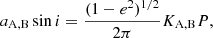
We list the orbital parameters of the system in the second column of Table 4, and we show in Fig. 1 the best fit to the RVs as a function of the orbital phase. Although the solution with non-zero eccentricity has a slightly better likelihood, it was not significantly different from a circular solution within the errors, putting a 1σ upper limit of e = 0.0017. Therefore, we decided to keep e sin ω and e cos ω fixed to zero. We found a sub-day orbital period of 0.60417356 d, with an uncertainty of less than 0.1 s, and a semi-amplitude of the RV signal of  km s−1. Given that the tidal circularisation timescale is small for orbital periods below 10 days, assuming a circular orbit for this system is further justified (Mazeh 2008). From this solution and the estimated mass of the primary component in Table 1, we solved Eq. (3) to obtain a minimum secondary mass of 0.0979 ± 0.0025 M⊙, which is equivalent to a minimum mass ratio of 0.2.
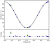 |
Fig. 1. Best orbital fit to the RVs of GJ 207.1 from CARMENES (blue circles), HARPS (red triangle), and FEROS (green squares), phase folded to the period of the system. Bottom panel: residuals from the fit. |
Computed and derived parameter for the SB1 systems.
We analysed the available photometric data listed in Table 2 to look for significant signals in the GLS periodograms. We found no significant periods in the ASAS photometry. However, as shown in the top panel of Fig. 2, we found very significant signals at 0.6042 ± 0.0012, 0.6043 ± 0.0003, and 0.60460 ± 0.00013 d in the TJO, SWASP, and TESS photometry, respectively, very similar to the orbital period of the system. We also found the same significant period at 0.605 ± 0.007 d when analysing the TESS data separately for sectors 6 and 32. After removal of the main signal, the residuals of the combined data still show an accumulation of significant peaks around 0.6 d. This accumulation could be an indication that the signal, while maintaining the same period, slightly changed its phase between the two sectors, producing an interference pattern in the periodogram. The periodograms of the residuals of the individual sectors, however, do not show any significant signal around 0.6 d, but they do at the first harmonic at about 0.3 d, as can be seen in the bottom panel of Fig. 2.
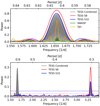 |
Fig. 2. GLS periodogram of the combined TESS data (grey) and their sectors 6 (red) and 32 (blue), SWASP (green), and TJO (orange) photometry of GJ 207.1 (top), and periodogram of the residuals of the combined TESS data (grey) and their sectors 6 (red) and 32 (blue) after the removal of the significant signals (bottom). The horizontal dotted lines of the corresponding colours indicate the corresponding 0.1% FAP level. |
Tidal evolution theory predicts that the synchronisation and alignment timescales should be two or three orders of magnitude shorter than the circularisation timescale (Zahn & Bouchet 1989; Mazeh 2008). Given that the orbit of GJ 207.1 is already circularised, and that the orbital and rotation periods are virtually identical, we expect that spin-orbit alignment should have already been achieved. If this is the case, we can estimate the orbital inclination by combining the measured v sin i (9.8 km −1; see Table 1) of the star together with the measured rotation period and the stellar radius. This yields a significantly pole-on orbital inclination of  deg, which results in a companion mass of
  M⊙ with an RV semi-amplitude of
  km s−1.
The measured v sin i of GJ 207.1 may be biased due to its short orbital period. During the exposure time of the spectroscopic observations, which varies between 8 and 30 min, we estimate that the RV shifts can reach up to 7.6 km s−1, depending on the orbital phase at which the observation was taken. This shift produces a broadening of the spectral lines that causes an overestimation of the true v sin i from the spectral analysis. However, we can estimate the effect of this RV shift over the measured v sin i taking into account that the variance of the observed line profile is the addition of the variances of the kernels defining the true line profile and the RV shift. The kernel of both the observed and true line profiles can be defined, to first order, by a Wigner semicircle distribution (Gray 2005) with radius equal to the projected rotational velocity and variance (v sin i)2/4, while the RV shift effect is defined by a rectangular function with length l equal to the shift and variance l2/12. Therefore, the true projected rotational velocity, vT sin i, is defined by  . Even in the worst-case scenario, where the RV shift caused by the exposure time is l = 7.6 km s−1, this equation yields a minimum value of vT sin i = 8.8 km s−1 which is well within the uncertainty of the measured v sin i = 9.8 ± 1.5 km s−1.
In general, the light curves of short-period binary systems present photometric modulations induced by the presence of a close companion. These include the reflection modulation and the beaming effect, which modulate the stellar brightness with orbital periodicity, and the ellipsoidal variation effect, which causes cyclic modulations at half the orbital period (Zucker et al. 2007; Mazeh 2008; Faigler & Mazeh 2011). These modulations can be approximated by sinusoidal functions, with harmonic periods and phase differences well defined with respect to the time of conjunction, and with constant amplitudes. These effects should be readily visible in the TESS photometry, but this appears to be dominated by activity-induced variations. This hypothesis is further favoured by the phase change observed between the two TESS sectors.
The theoretically predicted amplitudes of the Doppler beaming and ellipsoidal and reflection effects are ∼670, ∼780, and ∼0.7 ppm, as computed from Eq. (2) in Zucker et al. (2007) and Eqs. (2) and (3) in Faigler & Mazeh (2011). While we can neglect the reflection effect, the amplitudes of the Doppler beaming and ellipsoidal effect should be visible in the TESS photometry shown in Fig. 3, and therefore we can model them. To do so, we assumed the activity-induced variability to be a sinusoidal modulation at the orbital period (P = 0.60417356 d, Table 4) and different phases and amplitudes between the two sectors. To model the Doppler beaming and ellipsoidal effect, we assumed two cosine functions with periods P (for the Doppler beaming) and P/2 (for the ellipsoidal effect), with a reference time fixed to the maximum of the radial velocities and with the same amplitude in both sectors. The full model that we adopted to describe the variability in each TESS sector j is defined by
 (4)
(4)
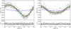 |
Fig. 3. Hourly binned photometry of GJ 207.1 from TESS sectors 6 (left) and 32 (right), phase folded to the orbital period. We show the best fit, described by Eq. (4), as a green solid line. The activity-induced variability is shown as a dash-dotted red line, while the magenta dotted line and the dashed blue line describe the ellipsoidal effect and the Doppler beaming, respectively. Bottom panels: residuals of the best fit. |
where aj and δj are the amplitude and phase of the activity-induced modulations in each sector, ab and ae are the amplitudes of the Doppler beaming and the ellipsoidal effect, and T is defined as t − tref, where tref is the time of maximum radial velocity. In addition to the orbital period, we also fixed the amplitude of the Doppler beaming modulation, since it depends on the well-constrained RV semi-amplitude KA, while we left C, δi, ai, and ae as free parameters. We computed the parameters and uncertainties by sampling the posterior probability distribution using emcee. The best-model fit is shown in Fig. 3. We obtain amplitudes of a6 = 4557 ± 67 ppm and a32 = 2023 ± 60 ppm for the activity-induced variability of TESS sectors 6 and 32, respectively, with a shift between them of 1.19 ± 0.03 rad. We obtained an amplitude of the ellipsoidal effect of ae = 694 ± 47 ppm, slightly lower than the predicted value of 780 ppm. From Eq. (2) in Faigler & Mazeh (2011), and using the computed ae and the estimated inclination, we derive a secondary mass of about 0.56 M⊙, which is in good agreement with the mass derived from RVs, within uncertainties. Since the photometric amplitude of the ellipsoidal effect is larger for inclinations closer to 90 deg, it is possible to put constraints on the inclination of the system independently of our former assumption about spin-orbit alignment. To do so, we estimated the amplitude ae at which the model is no longer compatible with the observed photometry. By setting a log-likelihood decrease of 15 with respect to the best-fit, we obtained the maximum ae amplitude at ∼1000 ppm. This upper limit rules out orbital inclinations higher than 20 deg, and therefore excludes companions with masses below 0.37 M⊙. For such a massive companion, the spectral lines of the two components of the system should be easily detected using todmor if it were a normal main-sequence M dwarf.
All the evidence points towards an underluminous companion to GJ 207.1 A. Interestingly, the absolute mass of the unseen component derived from the RVs under the assumption of zero obliquity of  M⊙ lies in the middle of the white dwarf mass distribution (Catalán et al. 2008). Therefore, we conclude that the secondary component of GJ 207.1 is most likely a white dwarf. We estimate that the progenitor star could have had a mass of
  M⊙, as computed from initial-to-final mass relationships (cf. Catalán et al. 2008). The time required for an object in this mass range to become a white dwarf is at least
  Ga (Marigo et al. 2001). However, the absolute masses and radii used to determine the mass of the white dwarf progenitor should be taken with caution. This binary system has probably suffered episodes of mass transfer during the red giant phase of the secondary, and the M dwarf could have truncated the evolution of the white dwarf precursor when it was ascending the giant branch. This truncation would produce a white dwarf with a lower mass than if it were isolated (Iben & Livio 1993; Rebassa-Mansergas et al. 2019), and may have changed the properties of both stars (Rebassa-Mansergas et al. 2011).
Bar et al. (2017) conducted a spectroscopic search for white dwarfs around nearby M dwarfs. For GJ 207.1, they set an upper limit of 8000 K for the temperature of any existing white dwarf in the system, estimated from the non-detection of any flux contribution from a companion in an X-shooter (Vernet et al. 2011) spectrum down to 300 nm. From the cooling sequences of hydrogen white dwarfs (Chabrier et al. 2000a) we estimate that it takes at least 1 Ga for a 0.6 M⊙ white dwarf to cool down to a temperature of ∼8000 K, and even more for more massive white dwarfs. All this evidence points towards an age older than 1 Ga for this system, in contradiction with the young age proposed in previous works (Lowrance et al. 2005).
To investigate this disagreement, we recomputed the Galactic space-velocity components determined by Montes et al. (2001) using the absolute RV of the system determined in this work and the newly available Gaia proper motions and parallax. These new parameters yield space velocity components U, V, and W of −21.4, −10.5, and −28.6 km s−1, respectively (Johnson & Soderblom 1987), which place the system in the thin disc population (Bensby et al. 2003), and outside the young disc population limits (Leggett 1992). Other stellar youth indicators for GJ 207.1, such as its UV and X-ray overluminosity, relatively strong Hα emission, and flaring activity can be explained by the fast rotation of the M-dwarf component caused by the spin-orbit synchronisation at the short orbital period of the binary. The characteristic age of the thin disc population is younger than ∼8 Ga (Fuhrmann 1998), which is compatible with the cooling age of the putative white dwarf. The upper limit of ∼8 Ga on the age, set by the kinematics of the system, and the lower limit of ∼1 Ga, set by the cooling time of the white dwarf, mean that the main-sequence phase of the progenitor star should not have lasted more than ∼7 Ga. Only stars with masses ≳0.9 M⊙ would reach the white dwarf stage within that time (Marigo et al. 2001) and would yield a final mass ≳0.52 M⊙ (Catalán et al. 2008).
4.1.2. GJ 912
GJ 912 is a high proper motion M2.5 V star located at a distance of 17.81 ± 0.03 pc. From its galactocentric space-velocity computed by Hawley et al. (1996), this system could be a member of the thin disc population, with an estimated age younger than 8 Ga (Fuhrmann 1998). No companions were found at angular separations between 0.1 arcsec and 3.5 arcsec with AstraLux (Jódar et al. 2013), or at wider separations using low-resolution imaging (Winters et al. 2019). The sensitivity of these surveys at small separations depended, however, on the flux ratio of the components. The rotation period estimated from the  index of the star, log(
 ) = − 5.01 ± 0.19, is of the order of 42 d (Astudillo-Defru et al. 2017).
Twenty-eight measurements for GJ 912 were obtained with CARMENES between July 2016 and November 2020. Nine archival observations from HARPS and three from FEROS taken between August 2009 and November 2013 are also available. An inspection of all the spectra with todmor revealed no secondary peaks in the CCF, indicating either an extreme flux ratio or a small relative RV between the two components. As for GJ 207.1, we used the difference between the CARMENES RVs computed with serval and with todmor to correct the offset of the FEROS todmor RVs.
The orbital parameters resulting from the MCMC analysis are shown in the third column of Table 4. The best-fit solution corresponds to a period of  d (about 14.2 a), with an RV semi-amplitude of
  km s−1. The orbit is highly eccentric,
  . The RVs and the best-fit solution are shown in Fig. 4 as a function of the orbital phase. Using the derived mass function f(M) and the estimated mass of the primary component (0.520 M⊙, Table 1), we determine a minimum companion mass of
  M⊙, which is compatible with a brown dwarf (i.e. mass lower than 0.072 M⊙, Chabrier et al. 2000b) for inclinations above ∼50 deg. Assuming an inclination probability distribution uniform in cos i (which implies a companion mass function favouring lower-mass companions), this corresponds to a probability of ∼63%. An inspection of the RV residuals of the best fit yielded no significant signals.
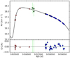 |
Fig. 4. Best orbital fit to the RVs of GJ 912 from CARMENES (blue circles), HARPS (red triangles), and FEROS (green squares) as a function of time. Residuals from the best fit are depicted in the bottom panel. Those corresponding to the FEROS observations are outside the Y-axis scale. |
We also analysed the available photometry of this object to search for signals of its rotation period. We binned the available SWASP data in nightly bins in order to reduce the scatter. Furthermore, we discarded observations made after BJD = 2 456 000 since they have systematical nightly deviations of more than three magnitudes, and the median of the errors is ten times higher than that of the previous data. This reduced the number of individual epochs in the light curve from 90 025 to only 256. The GLS periodogram shows a significant peak at 165 d. However, the long period was similar to the time span of each season of observation and, after its removal, a significant peak at 41.8 d arises, as shown in Fig. 5. Therefore, we attributed the 41.8 ± 1.3 d signal to the rotation period of the star, which is consistent with the period estimated by Astudillo-Defru et al. (2017). The error of the period was estimated from the width of the peak at half its maximum. No significant signals were found in the ASAS data. Based on the rotation period of this system, we can safely assume that this system is older than the objects of NGC 6811, with an estimated age of 1 Ga (Curtis et al. 2019a,b).
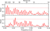 |
Fig. 5. GLS periodogram of the SWASP photometry of GJ 912 (top) and of the residuals after the removal of the significant signal (bottom). The horizontal dotted lines indicate the corresponding 0.1% FAP level. |
Finally, a constraint on the inclination of the system and, therefore, on the maximum mass of the companion, can be set by using 3.1 a of astrometric data from HIPPARCOS (Perryman et al. 1997; van Leeuwen 2007). In addition to the five standard astrometric parameters, we fitted an astrometric orbit to the HIPPARCOS abscissa residuals, from which the inclination and ascending node could be determined for GJ 912 via a least-squares minimisation (see Reffert & Quirrenbach 2011, for more details on the method). An astrometic orbit was detected with 94% probability, and the inclination was constrained to be greater than 5.5 deg at 1σ. An even more constraining limit can be set from the non-detection of a companion in the AstraLux observation by Jódar et al. (2013) made in August 2008. Assuming the 5 Ga stellar evolutionary model from Baraffe et al. (2015, hereafter BHAC15) and the estimated primary mass (0.520 ± 0.02 M⊙, Table 4), we converted the brightness contrast curve shown in Fig. 3 by Jódar et al. (2013) into mass detection limits, and show it in Fig. 6 as a function of the angular separation. We also show in Fig. 6 the minimum mass allowed by the radial velocities, and the range of possible angular separations between the components at the date of observation at any inclination between 0 and 90 deg. We can therefore determine that any companion with a mass above 0.21 M⊙ should be detected in the AstraLux observation, assuming that the companion is a main-sequence star. This limits the inclination to values higher than ∼17 deg, which pushes the probability of the secondary being a brown dwarf up to ∼66%.
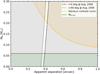 |
Fig. 6. Constraint on the mass of the secondary star in GJ 912 as a function of the apparent angular separation of the two components. The orange dashed line represents the contrast curve of the AstraLux observation by Jódar et al. (2013). The green solid line indicates the minimum mass limit computed from our RVs. The dashed and dotted black lines are constraints from RVs on the angular separation at the time of the observation, assuming inclinations between 0 deg (dashed) and 90 deg (dotted). The shaded regions indicate mass values that are not compatible with the observations. |
4.1.3. GJ 3626
Located at a distance of 22.61 ± 0.06 pc, GJ 3626 is an M4.0 V high proper motion star. It has a low activity level, with an Hα pseudo-equivalent width pEW(Hα) = +0.092 ± 0.014 Å (Schöfer et al. 2019), and an upper limit to the projected rotational velocity of 2 km s−1 (Reiners et al. 2018). No rotation period has been reported for this star. In the context of the sample selection of the CARMENES input catalogue, Cortés-Contreras et al. (2017) searched for low-mass companions to this star using the high-resolution lucky imaging instrument FastCam. From these observations, performed in March 2012, they excluded the presence of companions with ΔI < 4 mag between 0.2 and 2 arcsec, and with ΔI < 5 mag beyond 2 arcsec. In addition, observations taken for the Robo-AO adaptative optics M-dwarf multiplicity survey (Lamman et al. 2020), performed in January 2016, put limits on companions with Δi′< 2 mag beyond 0.1 arcsec, Δi′< 3 mag beyond 0.5 arcsec, and Δi′< 4 mag beyond 1 arcsec.
We observed GJ 3626 with CARMENES between March 2016 and November 2020, obtaining 42 spectra. We searched for the signature of a secondary component in the spectra using todmor, but no additional peaks in the CCF were detected. Therefore, we used the high-precision RVs computed with serval to determine the orbital parameters of the system as an SB1 However, to measure the absolute centre-of-mass RV, we used the RVs computed with todmor using synthetic spectra.
We show in Fig. 7 the best-fitting orbital solution; the parameters are listed in Table 4. The solution corresponds to a rather eccentric (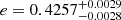 ) orbit with a period of
  d (about 8.24 a) and a semi-amplitude of
  km s−1. From the mass function computed from the fits and the primary component mass (0.403 ± 0.017 M⊙; Table 1), we calculate a minimum mass of
  M⊙ for the secondary component, well below the brown dwarf mass limit. We sampled the posterior distribution of minimum masses for 105 random values for the inclination, assuming a uniform distribution in cos i, and estimated a true secondary mass of
  M⊙ and an 87% chance of it being a brown dwarf.
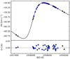 |
Fig. 7. Best orbital fit to the RVs of GJ 3626 from CARMENES as a function of time. The residuals from the fit are shown in the bottom panel. |
As an additional constraint, and as we did for GJ 912, we used the Robo-AO (Lamman et al. 2020) and the FastCam (Cortés-Contreras et al. 2017) contrast curves. Using the 5 Ga BHAC15 stellar evolutionary model and the estimated primary mass, we again converted the brightness contrast curves into mass detection limit, which are shown in Fig. 8 as a function of the orbital separation. We also illustrate in Fig. 8 the possible range of apparent angular separations of the two components, given any inclination between 0 and 90 deg, at the time of the FastCam and RoboAO observations. It can be seen from this figure that a companion with a mass above 0.11 M⊙ would have been detected in the FastCam observations. Using this limit as an upper bound to the companion mass, we set a lower bound to the inclination of the system to 19 deg, pushing the probability of the secondary component being a brown dwarf up to 93%.
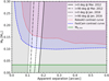 |
Fig. 8. Constraints on the mass of the secondary star in GJ 3626 as a function of the apparent angular separation of the two components. The red dotted and blue dashed lines represent the contrast curves of the Robo-AO and FastCam observations, respectively. The green solid line indicates the minimum mass limit computed from RVs. The solid and dot-dashed lines, and the dashed and dotted lines are constraints from RVs on the angular separation at the time of the FastCam and Robo-AO observations, respectively, for orbital inclinations between 0 and 90 deg. The shaded regions indicate mass values that are not compatible with the observations. |
We also analysed the available photometry from SWASP to look for signals induced by rotation. We first removed outliers using a 3σ clipping procedure and binned the light curve into nightly bins, resulting in 96 epochs between May 2004 and June 2007. The GLS periodogram shows a significant peak at 199 d. However, the photometry is divided into two different subsets of less than 200 days, with ∼1000 days in between, which makes the interpretation of this signal difficult. Therefore, it is unclear whether this signal may be due to rotation. As a further check, we analysed the residuals from the fits to the RV curve with GLS. The periodogram shows a peak at 72.7 d just below the 10% FAP level, much higher than our adopted 0.1% FAP threshold. We also analysed the CARMENES activity indicators in order to check if this signal is caused by stellar activity. However, none of the indicators have any significant peak at this period or at any other frequency.
4.1.4. LP 427–016
LP 427−016 is an M3.0 V star located at a distance of 22.98 ± 0.03 pc. From its galactocentric space velocity, it was classified as a member of the Local Association kinematic group (Cortés-Contreras 2016), with an estimated age between 10 and 150 Ma (Bell et al. 2015). The Hα emission shows low levels of chromospheric emission, pEW(Hα) = −0.10±0.01 Å, and the spectroscopic observations are consistent with slow rotation, v sin i < 2 km s−1 (Schöfer et al. 2019; Jeffers et al. 2018). Furthermore, Díez Alonso et al. (2019) reported a rotation period of 89.9 ± 2.0 d using ASAS photometry, although with a poor FAP of 1.8%. Considering its hypothetical young age, the star would be expected to be magnetically active (Terndrup et al. 2000; West et al. 2008; Fang et al. 2018) and to have a shorter rotation period (Barnes 2003; Curtis et al. 2019a). However, this is not supported by the measured activity indicators or the rotation period of this star, pointing towards an older age for this system than suggested by its kinematic assignation (see López-Santiago et al. 2009, for an assessment of the contamination by old stars in purely kinematic searches of members of nearby young moving groups).
No close companions with ΔI < 3 mag at an angular separation greater than 0.2 arcsec were found in observations from the FastCam high-resolution lucky imager (Cortés-Contreras et al. 2017). In addition, observations from the Robo-AO adaptive optics M-dwarf multiplicity survey (Lamman et al. 2020) ruled out companions with Δi′< 1 mag beyond 0.1 arcsec, and Δi′< 5 mag beyond 1 arcsec.
This object was spectroscopically observed with CARMENES for a total of 22 times, between March 2016 and November 2020. Two FEROS observations, obtained two years before those of CARMENES, are also available. The RVs for this system are listed in Table A.1, and shown in Fig. 9. The CARMENES RVs show an unambiguous long-term trend indicating binarity, but no companion was detected with todmor. In order to move the FEROS RVs to the same offset level as the CARMENES RVs, we again used the difference between the CARMENES RVs computed using todmor and serval. An attempt to determine the best orbital fit resulted in the MCMCs diverging towards long periods, as expected. The best circular orbit fit, shown in Fig. 9, corresponds to a period of ∼35 500 d (97 a), although the circular model is compatible (Δlnℒ < 15) with orbital periods between ∼6400 d (17.5 a) and ∼100 000 d (274 a). We therefore adopt 6400 d as the shortest possible period for a circular orbit, which yields a semi-amplitude of 0.25 km s−1 and a minimum secondary mass of 0.012 M⊙.
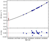 |
Fig. 9. Best fit to the RVs of LP 427−016 taken with CARMENES (blue circles) and FEROS (red triangle), assuming a circular orbit. Bottom panel: residuals from the fit. Those corresponding to FEROS observations are outside the Y-axis scale. |
More stringent bounds can be derived from the available observations with high-resolution imaging. Figure 10 shows the contrast curves obtained from the FastCam and Robo-AO high-resolution observations. We used the BHAC15 5 Ga evolutionary models to estimate the mass limit of the secondary component from the magnitude difference of the contrast curves and the mass of the primary component as for GJ 912. We also plot the minimum mass corresponding to the minimum allowed period derived from the RVs and the lower limit to the apparent separation (all assuming e = 0) computed with Kepler’s Third Law and the lower bound to the period. From this figure we conclude that any companion with a mass higher than ∼0.13 M⊙ would have been detected in high-resolution imaging observations. From this value, we obtain an upper bound to the period of ∼29 000 d (79 a). We suggest that the secondary component may have a mass in the range 0.011−0.13 M⊙, at an angular separation between 0.5 arcsec and 1.3 arcsec. We list in Table 4 all the limits to the orbital parameters resulting from this analysis.
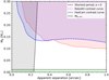 |
Fig. 10. Constraints on the mass of the secondary star in LP 427−016 as a function of the apparent separation of the two components. The red dotted and blue dashed lines depict the contrast curves of the RoboAO and FastCam observations, respectively. The green line indicates the minimum mass limit computed from RVs, of 0.011 M⊙. The black dashed line is the apparent separation for the lower limits to the period, assuming a circular orbit and i = 90 deg. The shaded regions indicate solutions that are not consistent with the observations. |
Allowing for non-zero eccentricity would affect the lower limit of the period, which could be as small as the time span of the data, ∼3000 d. Extreme values of the eccentricity would also allow very small apparent projected separations, increasing the upper limit to the mass of the companion.
LP 427−016 was photometrically monitored by the ASAS, NSVS, and SWASP surveys. As shown in Fig. 11, the GLS periodogram shows significant signals at periods of 33.2 ± 1.3 d and 38.9 ± 4.8 d for the NSVS and SWASP data, respectively, which are compatible within their errors. The second highest peak in the periodogram of the NSVS data, also significant and related to 33.2 ± 1.3 d by the window function, is at a period of 37.2 ± 1.3 d, coincident with the signal found in the SWASP data. In the ASAS data, we find excess power at a period of 89.9 d as claimed by Díez Alonso et al. (2019), but with a significance much lower than our 0.1% FAP threshold. Given that the time span of the SWASP data is five times longer than that of NSVS, although less precise, we attribute the 38.9 ± 4.8 d signal to the rotation period of the more massive star. As in the case of GJ 912, based on the rotation period of this system, we can safely assume that it is older than the objects of NGC 6811, with an estimated age of 1 Ga (Curtis et al. 2019a,b), and therefore rule out its membership to the Local Association kinematic group, as suggested by its space velocity, which, incidentally, could be biased by the binarity of the system.
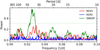 |
Fig. 11. GLS periodogram of the NSVS (red), ASAS (blue), and SWASP (green) photometry of LP 427−016. The horizontal dotted lines of each colour indicates the corresponding 0.1% FAP level. |
4.1.5. GJ 282 C
GJ 282 C is an M1.0 V star located at a distance of 14.23 ± 0.03 pc. It is active, with pEW(Hα) = −0.86 ± 0.01 Å (Schöfer et al. 2019), and also a bright X-ray source as observed by the ROSAT satellite (Voges et al. 1999; Kiraga 2012). Díez Alonso et al. (2019) reported a rotational period of 12.2 ± 0.1 d, based on ground-based photometry from ASAS. The projected rotational velocity is 3.1 ± 1.5 km s−1 (Reiners et al. 2018). Cortés-Contreras et al. (2017) observed this object with the FastCam high-resolution lucky imager, but no companions were detected. Poveda et al. (2009) determined that GJ 282 C is bound to the GJ 282 AB system, a pair of K3 V and K7 V stars (Reid et al. 1995; Montes et al. 2018), based on their small projected and radial separations, 55 300 and 25 000 au, respectively, their similar proper motions and RVs, and their identification as X-ray sources in the ROSAT catalogue. Nevertheless, Poveda et al. (2009) could not attribute the small discrepancies observed between the values of the proper motions and the RVs to the A–B orbit. From the kinematics of GJ 282 A, and therefore also GJ 282 C, Tabernero et al. (2017) classified this system as a member of the Ursa Major moving group, with an estimated age of about 300 Ma (Soderblom & Mayor 1993).
In recent years several works have published claims of the detection of a secondary companion to GJ 282 Ca (called GJ 282 Cb), although none of them provides a robust determination of the orbital parameters and masses. In order to determine the presence of perturbing objects in nearby stars, Kervella et al. (2019) searched for proper motion anomalies between the long-term proper motion vector, computed from the difference in the astrometric position between HIPPARCOS and Gaia and the proper motion measurements from the two catalogues. From this study, Kervella et al. (2019) obtained a lower limit to the secondary mass, normalised at an orbital radius of 1 au, of  MJup au−1/2. Furthermore, from high-contrast imaging observations made with NACO at the VLT, Kammerer et al. (2019) detected a companion at 441.5 ± 0.02 mas, with an Lp-band contrast of 2.619 ± 0.005 mag, which they classified as a candidate stellar-mass companion. Assuming a primary mass of 0.553 M⊙, as listed in Table 1, and using the 300 Ma BHAC15 models, this contrast would correspond to a ∼0.16 M⊙ companion. Finally, Grandjean et al. (2020) reported the detection of a low-mass stellar companion from the analysis of the HARPS RV data, in which they found a long-term trend with an amplitude of 700 m s−1 and also a short-term variation with an amplitude of 50 m s−1. Although they attributed the short-term variation to magnetic activity, they modelled the data with two Keplerian terms, obtaining a long period of 8500 ± 1900 d and an eccentricity of 0.55 ± 0.04, corresponding to a companion with a minimum mass of
  MJup, and a period of 22 d for the short-term signal. However, this short period is not consistent with the rotation period of 12.2 d reported from photometry (Díez Alonso et al. 2019), which would be the expected variability timescale for activity-related signals.
We observed GJ 282 C with CARMENES between January 2016 and November 2020, gathering a total of 42 spectra. Additionally, we retrieved 38 and 3 spectra from the HARPS and FEROS archives, respectively. A preliminary analysis of the RVs obtained with todmor revealed a clear long-period modulation with an amplitude of ∼4 km s−1. No signature of the companion was found in the spectra. As for the other systems, we used the difference between the CARMENES RVs derived with todmor and the RVs from serval, to correct the offset for the FEROS RVs, which could not be computed with serval. In addition to the RVs, we also analysed three high-contrast images acquired with NACO in January 2015, February 2016, and March 2016 to derive the angular separations and position angles of the two components, which we list in Table 3, together with the measured magnitude differences.
We simultaneously fitted the RVs and the differential astrometry using the code orvara, which also uses the acceleration on the plane of the sky from the HIPPARCOS−Gaia Catalog of Accelerations. To avoid systematic effects due to the different filters used in the astrometric observations, we scaled the errors of the separation and position angle listed in Table 3 by a constant value of 3.7 and 4.5, respectively, so that the reduced χ2 statistic of the astrometric fit was equal to one. The orbital parameters resulting from the MCMC analysis are listed in Table 5, and the best fit to the RVs and to the relative astrometric orbit are shown in Fig. 12. The best-fitting model has a period of  d with an eccentricity of
  , and an almost edge-on orbit with
 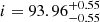 deg. From the computed orbital parameters, we derive absolute dynamical masses of
  M⊙ and
  M⊙ for the primary and secondary components, respectively. The mass of the primary is in agreement with the mass derived by Schweitzer et al. (2019) of 0.553 ± 0.02 M⊙ from empirical mass-luminosity calibrations. In addition, the luminosity contrast corresponding to these two masses in the L and K bands, estimated from the 300 Ma BHAC15 models, are 2.45 and 2.56, respectively, which are very similar to those computed from the NACO observations, listed in Table 3, although their filters do not exactly match those available from the models. The estimated contrast in the I band is 3.0, which lies right at the detection limit of the FastCam high-resolution imaging observations made in March 2014 by Cortés-Contreras et al. (2017), with a predicted angular separation of 500 mas. We find an additional significant signal at 12.1 d in the RV residuals of the best fit, which is in agreement with the rotation period found by Díez Alonso et al. (2019). No more significant signals are found in the data.
 |
Fig. 12. Best joint orbital fit to the spectroscopic data and differential astrometry of GJ 282 C. Left: RVs of GJ 282 C from CARMENES (blue cicles), HARPS (red triangles), and FEROS (green squares) as a function of time. The residuals from the fit are shown in the bottom panel, except for FEROS, which are outside the Y-axis scale. Right: differential astrometry between GJ 282 Ca and GJ 282 Cb. Orange circles show the astrometric relative position measured from NACO observations. The red cross gives the position of periastron, while the dashed line indicates the line of nodes. |
Orbital parameters for the astrometric binary GJ 282 C.
We analysed the available photometry, listed in Table 2, to search for rotational signals. As shown in the GLS periodograms in Fig. 13, we found significant periods at 12.15 ± 0.03 d, 12.21 ± 0.09 d, 12.27 ± 0.6 d, and 12.2 ± 2.5 d in the ASAS, SWASP, OSN, and TESS data, respectively, confirming the period found by Díez Alonso et al. (2019) using the ASAS photometry only. We also found short-period modulations of small amplitude in the TESS data, which could be produced by the companion. To compute their period, we fitted the TESS light curve with a GP, using a sum of two quasi-periodic kernels as a covariance function. We show the TESS photometry with the best-fit GP model in Fig. 14. We obtained periods of 12.41 ± 0.10 d and 0.32574 ± 0.00018 d for the large- and small-amplitude modulations, respectively. The estimated contribution of the companion to the total flux in the TESS band, based on the luminosity contrast measured by direct imaging, is around 3%. The short-period modulations, with an amplitude of 0.12% (see the middle panel of Fig. 14), could thus be explained by 4% modulations on the brightness of the companion. Another possibility is that the modulation is produced by a background star located within the TESS photometric mask around this object (Gaia EDR3 3060789275061364480). This star has a TESS-band magnitude of T = 12.0 mag, and it is thus brighter than GJ 282 Cb, which has an estimated T of ∼12.6 mag. The background star contributes with 7% of the global flux, which means that variations of 1.7% in its brightness would be required to produce the observed modulation. With an effective temperature for the background star of 6000 K estimated from Gaia data, such variations would be highly unusual (McQuillan et al. 2012). Given the young age and strong activity of GJ 282 C, we suggest that the short-period photometric signal is plausibly produced by the low-mass companion rather than the background star. We attribute the 12.2 d signal to the rotation of the primary component. In this case we adopt the period from the ASAS photometry because the light curve covers a large number of cycles, thus leading to a tighter constraint.
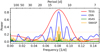 |
Fig. 13. GLS periodogram of the TESS (red), OSN (blue), ASAS (green), and SWASP (orange) photometry of GJ 282 C. The horizontal dotted line of each colour indicates the corresponding 0.1% FAP level. |
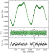 |
Fig. 14. TESS photometry of GJ 282 C with an hourly binning and the GP fit using as covariance function the sum of two quasi-periodic kernels, in green. The residuals of the TESS data and the best short-period GP model after subtracting the long-period model, and after subtracting the joint model are shown in the middle and bottom panels, respectively. |
Finally, using the systemic radial and astrometric properties derived from our analysis, listed in Table 5, we recalculated the galactocentric velocity, obtaining 25.1, −2.5, and −7.8 km s−1 for the U, V, and W components, respectively. These values are very similar to those of GJ 282 A listed by Tabernero et al. (2017) and compatible with members of the Ursa Major moving group (Montes et al. 2001), which supports the physical association of the quadruple system. Moreover, the pEW(Hα) of GJ 282 C is similar to or greater in absolute value than the values for members of the Hyades (∼650−800 Ma; Douglas et al. 2019, and references therein) measured by Terndrup et al. (2000) and Fang et al. (2018). Likewise, the X-ray luminosity log LX = 29.29 ± 0.17 erg s−1 (Voges et al. 1999) is also compatible with members of the Hyades (Núñez & Agüeros 2016), even if we assume that the Ca and Cb components have similar levels of X-ray emission. The rotational periods of GJ 282 Ca and Cb are longer than those measured by Rebull et al. (2016) for members of the Pleaides (∼110−130 Ma; Stauffer et al. 1998; Dahm 2015), but shorter than for the stars of Praesepe (∼600−750 Ma; Douglas et al. 2019, and references therein) as measured by Douglas et al. (2016). All this information supports the membership of GJ 282 C in the Ursa Major moving group, which makes this one of the youngest multiple stellar systems with known ages and dynamical masses (Lodieu et al. 2020). Furthermore, the masses are comparable with field objects of similar spectral type (Benedict et al. 2016, and references therein), which indicates that these low-mass stars in the mass range of 0.2−0.5 M⊙ have already arrived on the main sequence at the age of the moving group (Zapatero Osorio et al. 2014).
4.2. Double-line spectroscopic binaries (SB2s)
4.2.1. UCAC4 355–020729
UCAC4 355−020729 is an M5.0 V star located at a distance of 29.83 ± 0.03 pc. Catalogued as a bright X-ray source in the ROSAT bright source catalogue (Voges et al. 1999; Haakonsen & Rutledge 2009), it is an active star, with pEW(Hα) = −6.99 ± 0.04 Å, despite the relatively low value of its projected rotational velocity of 3.1 ± 1.5 km s−1.
We observed this system with CARMENES between November 2016 and November 2018, obtaining a total of 27 spectra. Although we could detect two signals in all spectra using todmor, the resulting RVs near the conjunctions were probably affected by systematics produced by blended lines due to the small RV difference between the two signals. We therefore removed these RVs from our orbital analysis. Table 6 lists the orbital parameters corresponding to the best-fitting solution to the RVs, while in Fig. 15 we show the RVs phase folded to the best orbital period. The best-fitting solution yields a slightly eccentric orbit, with e = 0.1123 ± 0.0054, and an orbital period of P = 6.56045 ± 0.00028 d. The semi-amplitudes of the RVs yield a mass ratio of  , and minimum masses of 3650 ± 61 × 10−8 M⊙ and 3136 ± 43 × 10−8 M⊙ for the primary and secondary components, respectively.
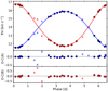 |
Fig. 15. todmor RV curves of UCAC4 355−020729 as a function of the orbital phase, along with their best-fitting models. The blue and red circles correspond to the primary and secondary components, respectively, while the crosses indicate data points not used in the fit. The residuals from the fit are shown in the bottom panels. |
Computed and derived parameters for the SB2 systems UU UMi and UCAC4 355−020729.
The very low minimum masses obtained could be an indication of an almost pole-on orientation of the orbit. Following the method described by Baroch et al. (2018), from the V-band magnitude of this system and the derived mass ratio listed in Table 6, and using the empirical mass-luminosity relation by Mann et al. (2019), we estimated the individual masses of the two components of the system, MA = 0.24 ± 0.02 and MB = 0.22 ± 0.02 M⊙. Using the obtained minimum masses, the orbital inclination should be lower than 3.0 deg. This low inclination would be consistent with the low value of the measured projected rotational velocity. This argument is even more convincing considering that this value is probably overestimated because of the blending of the spectral lines.
Finally, we analysed the photometry and activity indicators in search of stellar rotation signals, although the low inclination of the system is likely to greatly reduce the amplitude of a possible modulation. No significant signal was found in any of the activity indicators, aside from signals in the CRX and dLW that can be attributed to the blending of the two component spectra. The light curve from TESS (top panel of Fig. 16) reveals several flare events during the 27 days of continuous monitoring, as expected from the high activity of the star. After removing the flares with a sigma clipping and a rebinning of 1 h, the GLS periodogram (bottom panel of Fig. 16) shows three signals just above the 0.1% FAP level, at periods of 0.97, 1.46, and 2.82 d, which are not related to the 6.56 d period by any alias or harmonic. There are also no significant signals in the ASAS photometry.
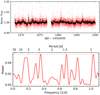 |
Fig. 16. Analysis of the TESS photometry of UCAC4 355−020729. Top panel: TESS photometry of UCAC4 355−020729 (red) and its one-hour binning (black). Bottom panel: GLS periodogram of the hourly binned TESS photometry. The horizontal dotted line indicates the 0.1% FAP level. |
4.2.2. UU UMi
Catalogued as the high proper motion star Ross 1057 (Ross 1939), UU UMi is an M3.0 V star located at a distance of 14.6 ± 0.3 pc. It is an inactive system, with pEW(Hα) = −0.10 ± 0.10 Å and a measured projected rotational velocity below 3 km s−1. Newton et al. (2016) reported a probable rotation period of 91 d from MEarth photometry, while Díez Alonso et al. (2019) found 83.4 ± 10.4 d using the same dataset. A first indication of its binarity was suggested by Lippincott (1981), who found evidence of variable proper motion in the residuals of plate series taken between 1970 and 1979, showing a perturbation with a period of 10−15 a and an amplitude of 0.04 arcsec. Heintz (1993) expanded the study including plates up to 1990, and found UU UMi to be an unresolved binary with a large astrometric variation amplitude and a companion mass of about 0.10 M⊙. The authors derived a circular orbit with a period of 14.5 a, an inclination of i = 92 deg, an amplitude of a = 0.0745 arcsec, and Ω = 21 deg.
The companion was detected spectroscopically in our previous study of binary systems discovered with the CARMENES instrument (Baroch et al. 2018), making this an SB2 system. We reported a mass ratio of 0.57 ± 0.06. However, from the modest fraction of the orbit covered by the data, the authors were not able to discern between a circular and an eccentric orbit, and therefore the eccentricity was fixed to zero. Here we update this analysis with eight additional CARMENES observations and one archival measurement taken with the CAFE spectrograph in May 2013. Although only the primary star can be resolved in this latter case, the almost equal RVs of the two spectra is useful information to constrain the systemic velocity and the time of conjunction. Table A.2 lists the full set of RVs used in this analysis for UU UMi.
From a Keplerian fit to the RVs of this system, which is shown in Fig. 17, we obtained a period of  d with an eccentricity of
  and a mass ratio of
  . The eccentric orbit is significantly favoured over a circular one, with a Bayesian information criterion (BIC) difference of 14 (strong evidence against the higher BIC value is obtained for ΔBIC > 6; Claeskens & Hjort 2008; Lillo-Box et al. 2014). Interestingly, the fitted period of
  a is in agreement with the value of 14.5 a found using astrometric observations by Heintz (1993). Using the almost edge-on inclination derived by Heintz (1993), i = 92 deg, we derived absolute masses of 0.32 ± 0.06 M⊙ and 0.19 ± 0.04 M⊙ for the primary and secondary components, respectively. Uncertainties on the mass may be underestimated because the inclination had no reported error bar.
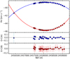 |
Fig. 17. Best fit to the todmor RVs of UU UMi as a function of time. Blue and red correspond to the primary and secondary components, respectively. Circular and triangular symbols correspond to the RVs from CARMENES and CAFE, respectively. The residuals from the best fit are shown in the bottom panels. |
We inspected the activity indices computed with serval to look for signs of stellar rotation, but without success. We also analysed TESS and ASAS photometry, equally unsuccesfully. In a GLS periodogram of the seven years of MEarth photometry, which we show in Fig. 18, we found a signal below the 0.1% FAP level at a period of 90 ± 10 d with an amplitude of 1 mmag, which was already reported by Newton et al. (2016) and Díez Alonso et al. (2019). This signal could be a product of the stellar rotation of one of the components and indicate an age of the system older than 1 Ga (Curtis et al. 2019a). Finally, we also reanalysed the HIPPARCOS photometry (Perryman et al. 1997) from which this object was catalogued as variable (Kazarovets et al. 1999; Adelman 2001). We found that all the points leading to the classification of UU UMi as a variable star are flagged as bad quality measurements.
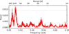 |
Fig. 18. GLS periodogram of the MEarth photometry of UU UMi. The horizontal dotted line indicates the corresponding 0.1% FAP level. |
4.3. Triple-line spectroscopic triples (ST3s)
4.3.1. GJ 3916
GJ 3916 is catalogued as an M2.0 V high proper motion star (Luyten 1955), located at a distance of 16.00 ± 0.07 pc. It is a quiet star, with pEW(Hα) = −0.03 ± 0.02 Å and a projected rotational velocity below 3 km s−1. Using empirical relationships, Astudillo-Defru et al. (2017) estimated a rotation period of 78 d from the emission strength of the Ca II H&K lines.
The first indication of the binarity of this system was deduced from HIPPARCOS astrometric data through the detection of an accelerated proper motion (Makarov & Kaplan 2005; Frankowski et al. 2007). More recently, Kervella et al. (2019) reported a difference in the proper motion between HIPPARCOS and Gaia, from which they obtained a lower limit to the secondary mass, normalised to an orbital separation of 1 au, of  MJup au−1/2. The presence of a companion to GJ 3916 was spectroscopically confirmed by Zechmeister et al. (2009), who reported a 4.1 km s−1 a−1 trend in six high-precision RVs obtained as part of the planet search programme with VLT+UVES (Dekker et al. 2000). Moreover, Houdebine & Mullan (2015) detected the signal of the secondary companion by cross-correlation in three high-resolution spectra taken with HARPS. They also obtained projected rotational velocities of 1.24 ± 0.14 and 3.51 ± 0.05 km s−1 for the primary and secondary signals, respectively.
we collected 32 spectra of GJ 3916 between April 2016 and August 2019 with CARMENES. We also used 23 spectra taken between March 2007 and July 2013 with the FEROS spectrograph, along with the UVES and HARPS spectra mentioned above. An inspection of the CARMENES spectra with todmor, using synthetic spectra, revealed a clear signal from a tertiary component in the system, in addition to the two expected signals. We proceeded as explained in Sect. 3.1 and extracted the RVs of the three signals in the spectra. We repeated the same process for the observations from UVES, FEROS, and HARPS, where the third signal was not as evident as in the CARMENES spectra. From the available 32 archival spectra, we could only detect all three signals in 11 spectra, two signals in 17 spectra, and only the signal from the brightest companion in 4. This effect was mostly due to the unfavourable orbital position of some of the components and the lower exposure time of the HARPS, UVES, and FEROS observations with respect to those from CARMENES. We list the RVs in Table A.3.
The RVs suggest a hierarchical triple system configuration, with the most massive star, A, tracing out a long-period orbit around the common barycentre with the two other stars, Ba and Bb, which in turn are orbiting each other with a shorter orbital period. The best fit to the hierarchical Keplerian model used to describe this system is shown in Fig. 19. The top panel depicts the RVs of the three components. In the middle panel we show the long-period orbit of components A around the Ba+Bb system after subtracting the RVs of the short-period orbit. In the bottom panel we show the orbital motion of Ba and Bb after subtracting the orbital motion of their centre of mass around component A. The fitted parameters are reported in Table 7. The outer orbit has a period of 3028 ± 23 d with an eccentricity of 0.458 ± 0.026, while the inner orbit has a period of  d and an eccentricity of
  . The minimum masses are
  ,
,  , and
, and  M⊙ for the components A, Ba, and Bb, respectively.
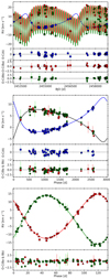 |
Fig. 19. Best fit to the RVs of GJ 3916. Top panel: fit to the RVs of the three components as a function of time. Middle panel: same fit, but phase folded to the period of the outer orbit and with the inner orbit subtracted. Bottom panel: fit to the inner orbit of the components Ba and Bb with outer orbit subtracted. The blue, red, and green symbols indicate the RVs of components A, Ba, and Bb, respectively. Measurements from CARMENES, FEROS, UVES, and HARPS are plotted as circular, squared, pentagonal, and triangular symbols, respectively. |
Computed and derived parameters for the ST3 systems GJ 3916 and GJ 4383.
Additionally, as we did for GJ 912, we constrained the inclination of the system by using the astrometric observations from HIPPARCOS. Following Reffert & Quirrenbach (2011) and using the orbital solution in Table 7, we fitted an astrometric orbit to the HIPPARCOS abscissa residuals, and determined an inclination of iAB = 99 ± 8 deg and an ascending node of Ω = 304 ± 8 deg at 1σ level. The astrometric orbit fitted here corresponds to the orbit of the photocentre, not of component A. As a result, the true apparent orbit would depend on the flux ratio between the most and least massive components (i.e. brightest and faintest), although this only affects the amplitude of the apparent orbit, and not the derived inclination. From the inclination of the outer orbit and the relation between sin iAB and sin iB we measured a difference between the inner and outer inclinations of Δi = 13 ± 7 deg, consistent with coplanarity within 2σ. We also used the estimated outer inclination, the minimum masses, and the mass ratios to assign absolute individual masses of 0.352 ± 0.047 M⊙, 0.195 ± 0.026 M⊙, and 0.174 ± 0.024 M⊙ for the A, Ba, and Bb components, respectively, which yields a mass ratio between the three components very close to 2:1:1.
We finally used the available photometry from ASAS and SWASP to search for signals of the rotation period of the components. No significant signals in the ASAS photometry could be detected, as was already reported by Díez Alonso et al. (2019). Although not significant, the highest peak in the periodogram of the SWASP data, shown in Fig. 20, is at ∼78 d, identical to the peak estimated by Astudillo-Defru et al. (2017) from the emission of the Ca II H&K lines. Using only the first two epochs of the SWASP data, which have half the dispersion and uncertainty of the rest, the peak at 78.1 ± 8.6 d becomes significant, and therefore we attribute it to the rotation period of star A, given the low expected flux of the other components.
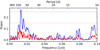 |
Fig. 20. GLS periodogram of the SWASP photometry of GJ 3916, using the entire dataset (red) and the first two epochs (blue). The horizontal dotted lines of each colour indicate the corresponding 0.1% FAP level. |
4.3.2. GJ 4383
GJ 4383 is an M3.0 V star located at a distance of 16.43 ± 0.07 pc. It is an inactive star, with pEW(Hα) = +0.04 ± 0.01 Å in absorption, and a projected rotational velocity lower than 2 km s−1. Using the measured  index, Astudillo-Defru et al. (2017) estimated a rotation period of 67 d, while Díez Alonso et al. (2019) did not find any significant signal in the ASAS photometry associated with rotation. Although the HIPPARCOS astrometry does not show an acceleration in the astrometric measurements, Makarov & Kaplan (2005) found discrepancies between the proper motions in the HIPPARCOS and Tycho-2 (Høg 2000) catalogues, and concluded that GJ 4383 could be an astrometric binary. Likewise, Kervella et al. (2019) found differences between the proper motions of HIPPARCOS and Gaia, from which a lower limit to the mass of the companion, normalised to 1 au, was set to
  MJup au−1/2.
We observed GJ 4383 with CARMENES between July 2016 and December 2020, gathering 26 high-resolution spectra. We also retrieved nine and four spectra from the HARPS and FEROS public databases, respectively. A first inspection of the spectra with todmor using synthetic spectra only revealed the signal of one component, whose RVs exhibit a sinusoidal shape, probably produced by a companion. To attempt to resolve the suspected companion, we used as templates the coadded spectra of the CARMENES observations of GJ 752 A and GJ 1253 (Sect. 3). With this approach, we resolved the signal of two additional components. From the 26 CARMENES spectra, we were able to detect the signal of the three components in 11 cases, two components in 10 spectra, and one component in 5. We did not detect the companions in any of the HARPS and FEROS spectra, mainly due to the lower exposure time of their observations with respect to those from CARMENES. We list the RVs in Table A.3.
The architecture of the RVs of this system is very similar to that of GJ 3916: two low-mass stars orbiting each other with a relatively short period, which in turn are orbiting a heavier star in a much wider orbit. We therefore fitted the same physical model to the RVs, which yielded the parameters listed in Table 7. We show in Fig. 21, from top to bottom, the orbital best fit to the RVs of GJ 4383 and the same fit phase folded to the A–B and Ba–Bb orbital periods. We measured a wide orbit between A and the pair Ba–Bb with an orbital period of 4646 ± 17 d and an eccentricity of 0.1068 ± 0.0049. The close orbit between the Ba and Bb components has a period of  d and an eccentricity of
  . From the derived semi-amplitudes we derived an approximately 4:1:1 mass ratio between the components, with minimum masses of
  M⊙,
M⊙,  M⊙, and
  M⊙ for components A, Ba, and Bb, respectively. The value of the minimum mass of component A deviates only 2σ from the value obtained from mass-luminosity calibrations of 0.455 ± 0.019 M⊙ by Schweitzer et al. (2019). This points to an almost edge-on orbit with respect to the line of sight.
Finally, we searched for significant signals in the available ASAS and SWASP photometry. No significant periods were found in the ASAS photometry. However, the periodogram of the SWASP photometry, shown in Fig. 22, has a significant signal at 52.5 ± 1.8 d, which we attributed to the rotation period of the most massive star, given the low expected flux of the other components.
 |
Fig. 22. GLS periodogram of the SWASP photometry of GJ 4383. The horizontal dotted line indicates the corresponding 0.1% FAP level. |
5. Discussion and conclusions
In this study we determined the orbital parameters of eight new multiple systems using high-precision RVs collected with CARMENES and from archival data, and refined the orbital parameters of UU UMi by adding additional observations with respect to the analysis presented by Baroch et al. (2018). Adaptive optics imaging data also permitted us to measure the absolute masses of the Ursa Major moving group members GJ 282 Ca and GJ 282 Cb with uncertainties of 10% and 3%, respectively, making it one of the youngest systems with measured dynamical masses.
The multiple stars presented here, along with the SB2s in Baroch et al. (2018), add up to a total of 17 stellar systems detected among the 349 M-dwarf stars monitored with the CARMENES spectrograph. The new binary systems can be used to update the M-dwarf multiplicity rate measured in other works. In a volume-limited sample of 1120 M dwarfs with distances below 25 pc, Winters et al. (2019) counted 265 multiple systems, from which they computed a multiplicity rate of 23.7 ± 1.3% uncorrected for observational biases. Their sample included all the systems in this work except for UCAC4 355−020729, GJ 282 C, and LP 427−016, and already tagged as multiple only the systems UU UMi and GJ 3916, based on the works by Heintz (1993) and Zechmeister et al. (2009), respectively. Adding GJ 282 C, and LP 427−016 to the sample (UCAC4 355−020729 is beyond 25 pc), and tagging as multiple the systems found in this work, we compute a new multiplicity rate of 24.2 ± 1.3% (271 multiple systems of 1122 stars). Furthermore, the companion to GJ 282 Ca, GJ 282 Cb, enlarges the list of 512 M-dwarf stars with measured masses between 0.1 and 0.3 M⊙ at distances d < 15 pc compiled by Winters et al. (2021), who already compiled the mass estimate of UU UMi B reported by Baroch et al. (2018).
We found that the GJ 207.1 system is probably composed of a white dwarf and an M dwarf. The short orbital period of about 14.5 h suggests that this system may have survived a common envelope phase due to the evolution of the massive star (Nebot Gómez-Morán et al. 2011). The two components may have started off in a much wider orbit, but the engulfment of the M dwarf by the envelope of the white dwarf progenitor caused drag forces that transported orbital angular momentum to the envelope, which was finally ejected. This process may have ended up shrinking and tidally locking the orbit to the present state (Nebot Gómez-Morán et al. 2011; Skinner et al. 2017). The number of white dwarf plus M-dwarf close binary systems is rapidly increasing thanks to large-scale surveys such as SDSS (Rebassa-Mansergas et al. 2016) and LAMOST (Ren et al. 2018). However, these short-period post-common-envelope systems, in which the optical light is dominated by the M dwarf, are very uncommon, comprising an estimated fraction of 0.03−0.18% of all M dwarfs (Law et al. 2012), as estimated from the detection of three such systems in a photometric survey of 45 000 M dwarfs. Only one white dwarf (in the system GJ 207.1, identified here) has been found among the ∼360 stars in the CARMENES sample (Reiners et al. 2018), a ratio higher than that estimated by Law et al. (2012), but compatible because of that small-number statistics. The higher ratio we found could be a by-product of the sensitivity difference between the methods used to detect white dwarfs, since their imprint over RVs should be in principle easier to detect than using photometry.
Although RV surveys have detected an abundance of exoplanets, the number of close brown dwarf companions is small, even though brown dwarfs should be more easily detected in comparable orbits given the larger RV signals that they produce. Several studies estimated a stellar-brown dwarf multiplicity fraction around 1% for a large range of primary masses and separations (Halbwachs et al. 2000; Marcy & Butler 2000; McCarthy & Zuckerman 2004; Metchev & Hillenbrand 2009; Kraus et al. 2011). This is also valid for M-dwarf primaries (Dieterich et al. 2012), as suggested by the small number of M-dwarf–brown dwarf systems found in the sample of Winters et al. (2019) (18 out of 1120 objects) or by the two system candidates found in this work among the ∼360 M dwarfs observed with CARMENES. Observational evidence points to a bimodal companion mass function (Grether & Lineweaver 2006) with a gap, also called the brown dwarf desert, at the intersection between the planetary and stellar-companion mass functions. The position of this minimum in the companion mass function seems to increase with the mass of the host star (Quirrenbach et al. 2019), and therefore objects with similar masses may have very different formation mechanisms (Armitage & Bonnell 2002; Matzner & Levin 2005). Although the masses of the brown dwarf candidates found in this work are not fully constrained, the low mass of the host stars and the highly eccentric orbits of the systems may indicate that they probably belong to the ‘stellar’ part of the companion mass function. If that is the case, we would expect the same metallicity as for their host stars, whereas planet-like objects might be metal rich (Maldonado & Villaver 2017; Quirrenbach et al. 2019). GJ 912 B and GJ 3626 B, with computed minimum masses of ∼60 MJup and ∼30 MJup, respectively, and expected angular separations between 100 mas and 300 mas, may be directly imaged with state-of-the-art imagers such as Gemini/GPI (Macintosh et al. 2014), Subaru/SCExAO (Jovanovic et al. 2015), Keck/OSIRIS-NIRC2 (Wizinowich et al. 2006; Larkin et al. 2006), or VLT/SPHERE (Beuzit et al. 2019), as estimated from simulated planet injections (Wagner et al. 2020). If the brown dwarf nature of GJ 912 B and GJ 3626 B is confirmed with future observations, they will help to better constrain the multiplicity rate of these systems and the boundaries of the brown dwarf desert, providing additional insights into the formation mechanisms of brown dwarfs.
Finally, we revealed the triple natures of two systems, GJ 3916 and GJ 4383, and were able to detect the spectroscopic signals of the three components for each system. Interestingly enough, the masses of the close inner pairs are nearly identical in both cases, and their combined mass is either equal to the outer component or half that value. These results could help to constrain formation models. Understanding the processes leading to the formation of multiple systems is one of the fundamental challenges in astrophysics, and has been a matter of debate for many years (Duchêne & Kraus 2013). One possible mechanism is the formation of these systems through the fragmentation of collapsing and rotating protostellar clouds (Boss 1988). Another possible explanation is the dynamical break-up of rapidly rotating clouds, or fission, although this mechanism does not seem to lead to the production of equal-mass binary protostars (Durisen et al. 1986), and thus is not capable of explaining the mass ratio distribution for binary systems, which shows an intrinsic excess at about unity (Lucy 2006; Simon & Obbie 2009). The formation of both democratic (all components with similar masses) and hierarchical systems could be explained by fragmentation. In the first case the cloud fragments into three or more protostars, while in the second case the cloud first collapses into binary protostars, which then can undergo subsequent fragmentations. Most observed triples have hierarchical structures, consisting of an inner binary and a distant star (Hut & Bahcall 1983; Tokovinin et al. 2006) because democratic triples tend to be unstable and short-lived (van den Berk et al. 2007). The presence of a third body on a wide orbit around a tight binary causes an angular momentum exchange between the two orbits, which in turn produces dynamical variations, such as periodic oscillations in the eccentricity of the inner binary and in the mutual inclination through Lidov-Kozai interactions (Lidov 1962; Kozai 1962; Mazeh & Shaham 1979; Naoz 2016). Usually, the timescale of such interactions is much longer than the orbital periods, and thus their effect in triple systems has only been detected indirectly through unusual inner eccentricity values (Kiseleva et al. 1998; Ford et al. 2000) or measured directly in very few systems (Jha et al. 2000). However, tight orbital configurations produce dynamical variations on timescales of the order of the orbital period, which lead to the disruption of the system.
In order to check the long-term stability of the triple systems found in this work we used the Eggleton & Kiseleva (1995) criterion for the stability of triple stellar systems, which He & Petrovich (2018) found to work reasonably well for a wide range of parameters in their N-body simulations. According to this criterion, the systems are stable when the orbit separation parameter  is higher than the value YEK defined as
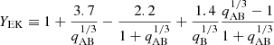 (5)
(5)
(Eggleton & Kiseleva 1995; He & Petrovich 2018).
For the cases of the triple systems GJ 3916 and GJ 4383, which have an orbit separation parameter rap of 5.03 and 7.89, we obtained values of YEK of 3.56 and 4.17, respectively. Therefore, both systems have stable orbital configurations.
The timescale of the Lidov-Kozai interactions is also useful for assessing the stability of the system. Actually, this parameter is crucial for verifying whether the orbit of the systems can be approximated by a Keplerian function in a hierarchical system during the time span of all the RV measurements, as we do in this work. This timescale τLK is defined as
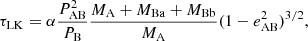 (6)
(6)
where α is close to one, and weakly depends on the orbital parameters (Kinoshita & Nakai 1999; Toonen et al. 2020). Equation (6) yields timescales of the Lidov-Kozai oscillations for GJ 3916 and GJ 4383 of 272 a and 414 a, respectively, which in both cases (just by chance) is equivalent to 33 orbital periods of the outer binary. The time span of the RV measurements used in the fits covered just 5.6% and a 2.3% of τLK for GJ 3916 and GJ 4383, respectively. This small fraction of the Lidov-Kozai cycle does not have a significant effect on the orbital fits of the RVs of these systems. This is also confirmed by the lack of systematic deviations in the residuals shown in the top panels of Figs. 19 and 21.
Figure 23 shows the mass ratios of the multiple systems found in this work and by Baroch et al. (2018) as a function of their orbital period. Apart from the lack of systems with mass ratios lower than ∼0.3, as expected from the flux ratio needed to distinguish between the two components in the spectra with todmor, no clear dependence on the orbital period of the systems can be observed. We do find, however, a dependence of the stellar activity on the orbital period: systems with periods shorter than ∼10 d have strong emission in the Hα line, whereas systems with longer periods have weak emission or even, in the earliest types, show the same spectral line in absorption. This is probably caused by the synchronisation between the rotation of the stars and the orbital motion due to tidal effects, which for main-sequence stars should be achieved for orbital periods below 8−10 d (Mazeh 2008). In addition, short rotation periods are associated with increased stellar activity in M dwarfs (Newton et al. 2016; Suárez Mascareño et al. 2016; Astudillo-Defru et al. 2017; Jeffers et al. 2018).
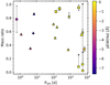 |
Fig. 23. Mass ratio as a function of the orbital period of the multiple systems characterised in this work and in Baroch et al. (2018), colour-coded by the pEW(Hα). The circular, triangular, and square symbols correspond to SB1, SB2, and ST3 systems, respectively. The upward arrows indicate the mass ratio limits for the systems for which only upper and lower bounds to the secondary masses could be given. The outer and inner orbits of the ST3 are plotted as individual binaries, with the same pEW(Hα). |
The determination of the spectroscopic orbits and properties of the systems in this work will provide help to understand the galactic population as a whole. The new systems contribute to statistical studies of stellar multiplicity and of the frequency of singular objects, and provide additional constraints on star formation theories, stellar evolutionary and structure models, and empirical calibrations. These constraints could be enhanced by the determination of the individual masses of the systems, which will be possible with the upcoming Gaia data releases containing the astrometric epoch data, and with the direct imaging of some of the systems.
Acknowledgments
Based on observations collected at the Centro Astronómico Hispano Alemán (CAHA) at Calar Alto, operated jointly by the Junta de Andalucía and the Instituto de Astrofísica de Andalucía (CSIC). CARMENES is funded by the German Max-Planck-Gesellschaft (MPG), the Spanish Consejo Superior de Investigaciones Científicas (CSIC), the European Union through FEDER/ERF FICTS-2011-02 funds, and the members of the CARMENES Consortium (Max-Planck-Institut für Astronomie, Instituto de Astrofísica de Andalucía, Landessternwarte Königstuhl, Institut de Ciències de l’Espai, Insitut für Astrophysik Göttingen, Universidad Complutense de Madrid, Thüringer Landessternwarte Tautenburg, Instituto de Astroísica de Canarias, Hamburger Sternwarte, Centro de Astrobiología and Centro Astronómico Hispano-Alemán), with additional contributions by the Spanish Ministry of Economy, the German Science Foundation through the Major Research Instrumentation Programme and DFG Research Unit FOR2544 ‘Blue Planets around Red Stars’, the Klaus Tschira Stiftung, the states of Baden-Württemberg and Niedersachsen, and by the Junta de Andalucía. Based on data from the CARMENES data archive at CAB (INTA-CSIC). Based on observations made with the 0.9-m telescope at the Sierra Nevada Observatory (Granada, Spain), operated by the Instituto de Astrofísica de Andalucía, the 0.8-m Joan Oró telescope (TJO) of the Montsec Astronomical Observatory (Lleida, Spain), owned by the Generalitat de Catalunya and operated by the Institut d’Estudis Espacials de Catalunya (IEEC), on observations collected at the European Southern Observatory under ESO programs 098.C-0739(A) and 192.C-0224(C) (P.I. A. M. Lagrange), 180.C-0886(A) and 183.C-0437(A) (P.I. X. Bonfils), 074.D-0016(A) (P.I. D. Montes), 078.A-9048(A) (P.I. J. Setiawan), 085.A-9027(A) (P.I. R. Gredel), 090.A-9003(A) and 091.A-9004(A) (P.I. R. Mundt), 173.C-0606(C) (P.I. M. Kürster), 096.D-0818(A) (P.I. K. Ward-Duong), 094.C-0625(A) and 097.C-0972(A) (P.I. J. H. Girard), and 081.A-9005(A), 081.A-9024(A), 083.A-9002(A), 083.A-9012(A,B), 085.A-9009(A), and 086.A-9016(A) (P.I. M. Zechmeister). This work has made use of data from the European Space Agency (ESA) mission Gaia (https://www.cosmos.esa.int/gaia), processed by the Gaia Data Processing and Analysis Consortium (DPAC, https://www.cosmos.esa.int/web/gaia/dpac/consortium). Funding for the DPAC has been provided by national institutions, in particular the institutions participating in the Gaia Multilateral Agreement. IRAF was distributed by the National Optical Astronomy Observatories, which is operated by the Association of Universities for Research in Astronomy, Inc. (AURA) under cooperative agreement with the National Science Foundation. We acknowledge financial support from the Spanish Agencia Estatal de Investigación of the Ministerio de Ciencia e Innovación (AEI-MCINN) and the European FEDER/ERF funds through projects PGC2018-098153-B-C33, PID2019-109522GB-C51/52/53/54, PID2019-107061GB-C64, ESP2017-87143-R, and the Centre of Excellence “Severo Ochoa” and “María de Maeztu” awards to the Instituto de Astrofísica de Canarias (SEV-2015-0548), Instituto de Astrofísica de Andalucía (SEV-2017-0709), and Centro de Astrobiología (MDM-2017-0737), the Secretaria d’Universitats i Recerca del Departament d’Empresa i Coneixement de la Generalitat de Catalunya and the Agència de Gestió d’Ajuts Universitaris i de Recerca of the Generalitat de Catalunya, with additional funding from the European FEDER/ERF funds, L’FSE inverteix en el teu futur, and from the Generalitat de Catalunya/CERCA programme.
References
- Aceituno, J., Sánchez, S. F., Grupp, F., et al. 2013, A&A, 552, A31 [NASA ADS] [CrossRef] [EDP Sciences] [Google Scholar]
- Adelman, S. J. 2001, Balt. Astron., 10, 589 [NASA ADS] [Google Scholar]
- Allard, F., Homeier, D., & Freytag, B. 2012, Phil. Trans. R. Soc. London Ser. A, 370, 2765 [Google Scholar]
- Alonso-Floriano, F. J., Morales, J. C., Caballero, J. A., et al. 2015, A&A, 577, A128 [NASA ADS] [CrossRef] [EDP Sciences] [Google Scholar]
- Andersen, J. 1991, A&ARv, 3, 91 [NASA ADS] [CrossRef] [Google Scholar]
- Anglada-Escudé, G., & Butler, R. P. 2012, ApJS, 200, 15 [NASA ADS] [CrossRef] [Google Scholar]
- Angus, R., Morton, T., Aigrain, S., Foreman-Mackey, D., & Rajpaul, V. 2018, MNRAS, 474, 2094 [NASA ADS] [CrossRef] [Google Scholar]
- Ansdell, M., Gaidos, E., Mann, A. W., et al. 2015, ApJ, 798, 41 [Google Scholar]
- Armitage, P. J., & Bonnell, I. A. 2002, MNRAS, 330, L11 [NASA ADS] [CrossRef] [Google Scholar]
- Astudillo-Defru, N., Delfosse, X., Bonfils, X., et al. 2017, A&A, 600, A13 [NASA ADS] [CrossRef] [EDP Sciences] [Google Scholar]
- Baluev, R. V. 2009, MNRAS, 393, 969 [NASA ADS] [CrossRef] [Google Scholar]
- Bar, I., Vreeswijk, P., Gal-Yam, A., Ofek, E. O., & Nelemans, G. 2017, ApJ, 850, 34 [NASA ADS] [CrossRef] [Google Scholar]
- Baraffe, I., Homeier, D., Allard, F., & Chabrier, G. 2015, A&A, 577, A42 [NASA ADS] [CrossRef] [EDP Sciences] [Google Scholar]
- Barnes, S. A. 2003, ApJ, 586, 464 [NASA ADS] [CrossRef] [Google Scholar]
- Baroch, D., Morales, J. C., Ribas, I., et al. 2018, A&A, 619, A32 [NASA ADS] [CrossRef] [EDP Sciences] [Google Scholar]
- Bell, C. P. M., Mamajek, E. E., & Naylor, T. 2015, MNRAS, 454, 593 [NASA ADS] [CrossRef] [Google Scholar]
- Benedict, G. F., Henry, T. J., Franz, O. G., et al. 2016, AJ, 152, 141 [NASA ADS] [CrossRef] [Google Scholar]
- Bensby, T., Feltzing, S., & Lundström, I. 2003, A&A, 410, 527 [NASA ADS] [CrossRef] [EDP Sciences] [Google Scholar]
- Berta, Z. K., Irwin, J., Charbonneau, D., Burke, C. J., & Falco, E. E. 2012, AJ, 144, 145 [NASA ADS] [CrossRef] [Google Scholar]
- Beuzit, J. L., Vigan, A., Mouillet, D., et al. 2019, A&A, 631, A155 [NASA ADS] [CrossRef] [EDP Sciences] [Google Scholar]
- Biller, B. A., Close, L. M., Masciadri, E., et al. 2007, ApJS, 173, 143 [NASA ADS] [CrossRef] [Google Scholar]
- Boss, A. P. 1988, Comments Astrophys., 12, 169 [NASA ADS] [Google Scholar]
- Brandt, T. D. 2018, ApJS, 239, 31 [NASA ADS] [CrossRef] [Google Scholar]
- Brandt, T. D., Dupuy, T. J., & Li, Y. 2021, AJ, submitted [arXiv: 2105.11671] [Google Scholar]
- Caballero, J. A., Guàrdia, J., López del Fresno, M., et al. 2016, Proc. SPIE, 9910, 99100E [Google Scholar]
- Catalán, S., Isern, J., García-Berro, E., & Ribas, I. 2008, MNRAS, 387, 1693 [NASA ADS] [CrossRef] [Google Scholar]
- Chabrier, G., Brassard, P., Fontaine, G., & Saumon, D. 2000a, ApJ, 543, 216 [NASA ADS] [CrossRef] [Google Scholar]
- Chabrier, G., Baraffe, I., Allard, F., & Hauschildt, P. 2000b, ApJ, 542, 464 [Google Scholar]
- Claeskens, G., & Hjort, N. L. 2008, Model Selection and Model Averaging, Cambridge Series in Statistical and Probabilistic Mathematics (Leiden: Cambridge Univ. Press) [Google Scholar]
- Cortés-Contreras, M. 2016, PhD Thesis, Universidad Complutense de Madrid [Google Scholar]
- Cortés-Contreras, M., Béjar, V. J. S., Caballero, J. A., et al. 2017, A&A, 597, A47 [NASA ADS] [CrossRef] [EDP Sciences] [Google Scholar]
- Curtis, J. L., Agüeros, M. A., Mamajek, E. E., Wright, J. T., & Cummings, J. D. 2019a, AJ, 158, 77 [NASA ADS] [CrossRef] [Google Scholar]
- Curtis, J. L., Agüeros, M. A., Douglas, S. T., & Meibom, S. 2019b, ApJ, 879, 49 [NASA ADS] [CrossRef] [Google Scholar]
- Dahm, S. E. 2015, ApJ, 813, 108 [NASA ADS] [CrossRef] [Google Scholar]
- Dekker, H., D’Odorico, S., Kaufer, A., Delabre, B., & Kotzlowski, H. 2000, in SPIE Conf. Ser., eds. M. Iye, & A. F. Moorwood, Proc. SPIE, 4008, 534 [Google Scholar]
- Dieterich, S. B., Henry, T. J., Golimowski, D. A., Krist, J. E., & Tanner, A. M. 2012, AJ, 144, 64 [Google Scholar]
- Díez Alonso, E., Caballero, J. A., Montes, D., et al. 2019, A&A, 621, A126 [NASA ADS] [CrossRef] [EDP Sciences] [Google Scholar]
- Douglas, S. T., Agüeros, M. A., Covey, K. R., et al. 2016, ApJ, 822, 47 [NASA ADS] [CrossRef] [Google Scholar]
- Douglas, S. T., Curtis, J. L., Agüeros, M. A., et al. 2019, ApJ, 879, 100 [NASA ADS] [CrossRef] [Google Scholar]
- Dressing, C. D., & Charbonneau, D. 2013, ApJ, 767, 95 [NASA ADS] [CrossRef] [Google Scholar]
- Duchêne, G., & Kraus, A. 2013, ARA&A, 51, 269 [Google Scholar]
- Durisen, R. H., Gingold, R. A., Tohline, J. E., & Boss, A. P. 1986, ApJ, 305, 281 [CrossRef] [Google Scholar]
- Eggen, O. J. 1956, AJ, 61, 405 [NASA ADS] [CrossRef] [Google Scholar]
- Eggleton, P., & Kiseleva, L. 1995, ApJ, 455, 640 [NASA ADS] [CrossRef] [Google Scholar]
- Faigler, S., & Mazeh, T. 2011, MNRAS, 415, 3921 [Google Scholar]
- Fang, X.-S., Zhao, G., Zhao, J.-K., & Bharat Kumar, Y. 2018, MNRAS, 476, 908 [NASA ADS] [CrossRef] [Google Scholar]
- Feiden, G. A., & Chaboyer, B. 2014, A&A, 571, A70 [NASA ADS] [CrossRef] [EDP Sciences] [Google Scholar]
- Ford, E. B., Kozinsky, B., & Rasio, F. A. 2000, ApJ, 535, 385 [NASA ADS] [CrossRef] [Google Scholar]
- Foreman-Mackey, D., Hogg, D. W., Lang, D., & Goodman, J. 2013, PASP, 125, 306 [Google Scholar]
- Frankowski, A., Jancart, S., & Jorissen, A. 2007, A&A, 464, 377 [NASA ADS] [CrossRef] [EDP Sciences] [Google Scholar]
- Fuhrmann, K. 1998, A&A, 338, 161 [NASA ADS] [Google Scholar]
- Gaia Collaboration (Prusti, T., et al.) 2016, A&A, 595, A1 [NASA ADS] [CrossRef] [EDP Sciences] [Google Scholar]
- Gaia Collaboration (Brown, A. G. A., et al.) 2018, A&A, 616, A1 [NASA ADS] [CrossRef] [EDP Sciences] [Google Scholar]
- Gaia Collaboration (Brown, A. G. A., et al.) 2021, A&A, 649, A1 [NASA ADS] [CrossRef] [EDP Sciences] [Google Scholar]
- Gizis, J. E., Reid, I. N., & Hawley, S. L. 2002, AJ, 123, 3356 [Google Scholar]
- Goodman, J., & Weare, J. 2010, Commun. Appl. Math. Comput. Sci., 5, 65 [Google Scholar]
- Grandjean, A., Lagrange, A. M., Keppler, M., et al. 2020, A&A, 633, A44 [NASA ADS] [CrossRef] [EDP Sciences] [Google Scholar]
- Gray, D. F. 2005, The Observation and Analysis of Stellar Photospheres (Cambridge: Cambridge University Press) [CrossRef] [Google Scholar]
- Grether, D., & Lineweaver, C. H. 2006, ApJ, 640, 1051 [NASA ADS] [CrossRef] [Google Scholar]
- Haakonsen, C. B., & Rutledge, R. E. 2009, ApJS, 184, 138 [NASA ADS] [CrossRef] [Google Scholar]
- Halbwachs, J. L., Arenou, F., Mayor, M., Udry, S., & Queloz, D. 2000, A&A, 355, 581 [Google Scholar]
- Hawley, S. L., Gizis, J. E., & Reid, I. N. 1996, AJ, 112, 2799 [NASA ADS] [CrossRef] [Google Scholar]
- He, M. Y., & Petrovich, C. 2018, MNRAS, 474, 20 [NASA ADS] [CrossRef] [Google Scholar]
- Heintz, W. D. 1993, AJ, 105, 1188 [NASA ADS] [CrossRef] [Google Scholar]
- Henry, T. J., Jao, W.-C., Subasavage, J. P., et al. 2006, AJ, 132, 2360 [NASA ADS] [CrossRef] [Google Scholar]
- Hilditch, R. W. 2001, An Introduction to Close Binary Stars (Cambridge: Cambridge University Press), 355 [CrossRef] [Google Scholar]
- Høg, E. 2000, in Tycho Star Catalogs: The 2.5 Million Brightest Stars, ed. P. Murdin, 2862 [Google Scholar]
- Houdebine, E. R., & Mullan, D. J. 2015, ApJ, 801, 106 [NASA ADS] [CrossRef] [Google Scholar]
- Husser, T. O., Wende-von Berg, S., Dreizler, S., et al. 2013, A&A, 553, A6 [NASA ADS] [CrossRef] [EDP Sciences] [Google Scholar]
- Hut, P., & Bahcall, J. N. 1983, ApJ, 268, 319 [NASA ADS] [CrossRef] [Google Scholar]
- Iben, I., Jr., & Livio, M. 1993, PASP, 105, 1373 [Google Scholar]
- Jeffers, S. V., Schöfer, P., Lamert, A., et al. 2018, A&A, 614, A76 [NASA ADS] [CrossRef] [EDP Sciences] [Google Scholar]
- Jha, S., Torres, G., Stefanik, R. P., Latham, D. W., & Mazeh, T. 2000, MNRAS, 317, 375 [NASA ADS] [CrossRef] [Google Scholar]
- Jódar, E., Pérez-Garrido, A., Díaz-Sánchez, A., et al. 2013, MNRAS, 429, 859 [NASA ADS] [CrossRef] [Google Scholar]
- Johnson, D. R. H., & Soderblom, D. R. 1987, AJ, 93, 864 [NASA ADS] [CrossRef] [Google Scholar]
- Jovanovic, N., Martinache, F., Guyon, O., et al. 2015, PASP, 127, 890 [NASA ADS] [CrossRef] [Google Scholar]
- Kammerer, J., Ireland, M. J., Martinache, F., & Girard, J. H. 2019, MNRAS, 486, 639 [NASA ADS] [CrossRef] [EDP Sciences] [Google Scholar]
- Kasting, J. F., Whitmire, D. P., & Reynolds, R. T. 1993, Icarus, 101, 108 [Google Scholar]
- Kaufer, A., Stahl, O., Tubbesing, S., et al. 1999, The Messenger, 95, 8 [Google Scholar]
- Kazarovets, E. V., Samus, N. N., Durlevich, O. V., et al. 1999, Inf. Bull. Var. Stars, 4659, 1 [Google Scholar]
- Kervella, P., Arenou, F., Mignard, F., & Thévenin, F. 2019, A&A, 623, A72 [NASA ADS] [CrossRef] [EDP Sciences] [Google Scholar]
- Kinoshita, H., & Nakai, H. 1999, Celest. Mech. Dyn. Astron., 75, 125 [NASA ADS] [CrossRef] [Google Scholar]
- Kiraga, M. 2012, Acta Astron., 62, 67 [NASA ADS] [Google Scholar]
- Kirk, B., Conroy, K., Prša, A., et al. 2016, AJ, 151, 68 [NASA ADS] [CrossRef] [Google Scholar]
- Kiseleva, L. G., Eggleton, P. P., & Mikkola, S. 1998, MNRAS, 300, 292 [NASA ADS] [CrossRef] [Google Scholar]
- Kopparapu, R. K., Ramirez, R., Kasting, J. F., et al. 2013, ApJ, 765, 131 [NASA ADS] [CrossRef] [Google Scholar]
- Kozai, Y. 1962, AJ, 67, 591 [Google Scholar]
- Kraus, A. L., Ireland, M. J., Martinache, F., & Hillenbrand, L. A. 2011, ApJ, 731, 8 [Google Scholar]
- Lamman, C., Baranec, C., Berta-Thompson, Z. K., et al. 2020, AJ, 159, 139 [CrossRef] [Google Scholar]
- Lampton, M., Lieu, R., Schmitt, J. H. M. M., et al. 1997, ApJS, 108, 545 [NASA ADS] [CrossRef] [Google Scholar]
- Larkin, J., Barczys, M., Krabbe, A., et al. 2006, in SPIE Conf. Ser., eds. I. S. McLean, & M. Iye, 6269, 62691A [NASA ADS] [Google Scholar]
- Law, N. M., Kraus, A. L., Street, R., et al. 2012, ApJ, 757, 133 [NASA ADS] [CrossRef] [Google Scholar]
- Leggett, S. K. 1992, ApJS, 82, 351 [NASA ADS] [CrossRef] [Google Scholar]
- Lenzen, R., Hartung, M., Brandner, W., et al. 2003, in SPIE Conf. Ser., eds. M. Iye, & A. F. M. Moorwood, Proc. SPIE, 4841, 944 [Google Scholar]
- Lépine, S., Hilton, E. J., Mann, A. W., et al. 2013, AJ, 145, 102 [NASA ADS] [CrossRef] [Google Scholar]
- Lidov, M. L. 1962, Planet. Space Sci., 9, 719 [Google Scholar]
- Lillo-Box, J., Barrado, D., Moya, A., et al. 2014, A&A, 562, A109 [NASA ADS] [CrossRef] [EDP Sciences] [Google Scholar]
- Lippincott, S. L. 1981, AJ, 86, 1401 [NASA ADS] [CrossRef] [Google Scholar]
- Lodieu, N., Paunzen, E., & Zejda, M. 2020, Low-Mass and Sub-stellar Eclipsing Binaries in Stellar Clusters (Cham: Springer), 213 [Google Scholar]
- López-Santiago, J., Micela, G., & Montes, D. 2009, A&A, 499, 129 [CrossRef] [Google Scholar]
- Lowrance, P. J., Becklin, E. E., Schneider, G., et al. 2005, AJ, 130, 1845 [NASA ADS] [CrossRef] [Google Scholar]
- Lucy, L. B. 2006, A&A, 457, 629 [NASA ADS] [CrossRef] [EDP Sciences] [Google Scholar]
- Luyten, W. J. 1955, Luyten’s Five Tenths [Google Scholar]
- Macintosh, B., Graham, J. R., Ingraham, P., et al. 2014, Proc. Natl. Acad. Sci., 111, 12661 [NASA ADS] [CrossRef] [Google Scholar]
- Makarov, V. V., & Kaplan, G. H. 2005, AJ, 129, 2420 [Google Scholar]
- Maldonado, J., & Villaver, E. 2017, A&A, 602, A38 [NASA ADS] [CrossRef] [EDP Sciences] [Google Scholar]
- Mann, A. W., Dupuy, T., Kraus, A. L., et al. 2019, ApJ, 871, 63 [NASA ADS] [CrossRef] [Google Scholar]
- Marcy, G. W., & Butler, R. P. 2000, PASP, 112, 137 [NASA ADS] [CrossRef] [Google Scholar]
- Marigo, P., Girardi, L., Chiosi, C., & Wood, P. R. 2001, A&A, 371, 152 [NASA ADS] [CrossRef] [EDP Sciences] [Google Scholar]
- Matzner, C. D., & Levin, Y. 2005, ApJ, 628, 817 [NASA ADS] [CrossRef] [Google Scholar]
- Mayor, M., Pepe, F., Queloz, D., et al. 2003, The Messenger, 114, 20 [NASA ADS] [Google Scholar]
- Mazeh, T. 2008, in EAS Pub. Ser., eds. M. J. Goupil, & J. P. Zahn, 29, 1 [Google Scholar]
- Mazeh, T., & Shaham, J. 1979, A&A, 77, 145 [Google Scholar]
- McCarthy, C., & Zuckerman, B. 2004, AJ, 127, 2871 [NASA ADS] [CrossRef] [Google Scholar]
- McQuillan, A., Aigrain, S., & Roberts, S. 2012, A&A, 539, A137 [NASA ADS] [CrossRef] [EDP Sciences] [Google Scholar]
- Metchev, S. A., & Hillenbrand, L. A. 2009, ApJS, 181, 62 [Google Scholar]
- Montes, D., López-Santiago, J., Gálvez, M. C., et al. 2001, MNRAS, 328, 45 [NASA ADS] [CrossRef] [MathSciNet] [Google Scholar]
- Montes, D., González-Peinado, R., Tabernero, H. M., et al. 2018, MNRAS, 479, 1332 [Google Scholar]
- Morales, J. C., Gallardo, J., Ribas, I., et al. 2010, ApJ, 718, 502 [NASA ADS] [CrossRef] [Google Scholar]
- Morales, J. C., Mustill, A. J., Ribas, I., et al. 2019, Science, 365, 1441 [NASA ADS] [CrossRef] [Google Scholar]
- Naoz, S. 2016, ARA&A, 54, 441 [Google Scholar]
- Nebot Gómez-Morán, A., Gänsicke, B. T., Schreiber, M. R., et al. 2011, A&A, 536, A43 [CrossRef] [Google Scholar]
- Newton, E. R., Irwin, J., Charbonneau, D., et al. 2016, ApJ, 821, 93 [NASA ADS] [CrossRef] [Google Scholar]
- Núñez, A., & Agüeros, M. A. 2016, ApJ, 830, 44 [Google Scholar]
- Passegger, V. M., Reiners, A., Jeffers, S. V., et al. 2018, A&A, 615, A6 [NASA ADS] [CrossRef] [EDP Sciences] [Google Scholar]
- Passegger, V. M., Bello-García, A., Ordieres-Meré, J., et al. 2020, A&A, 642, A22 [NASA ADS] [CrossRef] [EDP Sciences] [Google Scholar]
- Perryman, M. A. C., Lindegren, L., Kovalevsky, J., et al. 1997, A&A, 500, 501 [NASA ADS] [Google Scholar]
- Pojmanski, G. 1997, Acta Astron., 47, 467 [Google Scholar]
- Pollacco, D. L., Skillen, I., Collier Cameron, A., et al. 2006, PASP, 118, 1407 [NASA ADS] [CrossRef] [Google Scholar]
- Pounds, K. A., Allan, D. J., Barber, C., et al. 1993, MNRAS, 260, 77 [NASA ADS] [Google Scholar]
- Poveda, A., Allen, C., Costero, R., Echevarría, J., & Hernández-Alcántara, A. 2009, ApJ, 706, 343 [Google Scholar]
- Quirrenbach, A., Amado, P. J., Caballero, J. A., et al. 2014, Proc. SPIE, 9147, 91471F [Google Scholar]
- Quirrenbach, A., Amado, P. J., Caballero, J. A., et al. 2016, Proc. SPIE, 9908, 990812 [Google Scholar]
- Quirrenbach, A., Amado, P. J., & Ribas, I. 2018, in Ground-based and Airborne Instrumentation for Astronomy VII, eds. C. J. Evans, L. Simard, & H. Takami, SPIE Conf. Ser., 10702, 107020W [Google Scholar]
- Quirrenbach, A., Trifonov, T., Lee, M. H., & Reffert, S. 2019, A&A, 624, A18 [NASA ADS] [CrossRef] [EDP Sciences] [Google Scholar]
- Quirrenbach, A., CARMENES Consortium, Amado, P. J., et al. 2020, SPIE Conf. Ser., 11447, 114473C [Google Scholar]
- Rasmussen, C. E., & Williams, C. K. I. 2006, Gaussian Processes for Machine Learning, Adaptive Computation and Machine Learning (MIT Press), 1 [Google Scholar]
- Rebassa-Mansergas, A., Nebot Gómez-Morán, A., Schreiber, M. R., Girven, J., & Gänsicke, B. T. 2011, MNRAS, 413, 1121 [NASA ADS] [CrossRef] [Google Scholar]
- Rebassa-Mansergas, A., Ren, J. J., Parsons, S. G., et al. 2016, MNRAS, 458, 3808 [NASA ADS] [CrossRef] [Google Scholar]
- Rebassa-Mansergas, A., Parsons, S. G., Dhillon, V. S., et al. 2019, Nat. Astron., 3, 553 [NASA ADS] [CrossRef] [EDP Sciences] [Google Scholar]
- Rebull, L. M., Stauffer, J. R., Bouvier, J., et al. 2016, AJ, 152, 113 [NASA ADS] [CrossRef] [Google Scholar]
- Reffert, S., & Quirrenbach, A. 2011, A&A, 527, A140 [NASA ADS] [CrossRef] [EDP Sciences] [Google Scholar]
- Reid, I. N., Hawley, S. L., & Gizis, J. E. 1995, AJ, 110, 1838 [NASA ADS] [CrossRef] [Google Scholar]
- Reiners, A., Joshi, N., & Goldman, B. 2012, AJ, 143, 93 [NASA ADS] [CrossRef] [Google Scholar]
- Reiners, A., Zechmeister, M., Caballero, J. A., et al. 2018, A&A, 612, A49 [NASA ADS] [CrossRef] [EDP Sciences] [Google Scholar]
- Ren, J. J., Rebassa-Mansergas, A., Parsons, S. G., et al. 2018, MNRAS, 477, 4641 [NASA ADS] [CrossRef] [Google Scholar]
- Ribas, I., Tuomi, M., Reiners, A., et al. 2018, Nature, 563, 365 [NASA ADS] [CrossRef] [Google Scholar]
- Ricker, G. R., Winn, J. N., Vanderspek, R., et al. 2015, J. Astron. Telesc. Instrum. Syst., 1, 014003 [Google Scholar]
- Rodríguez, E., García, J. M., Costa, V., et al. 2010, MNRAS, 408, 2149 [NASA ADS] [CrossRef] [Google Scholar]
- Ross, F. E. 1939, AJ, 48, 163 [NASA ADS] [CrossRef] [EDP Sciences] [Google Scholar]
- Rousset, G., Lacombe, F., Puget, P., et al. 2003, in SPIE Conf. Ser., eds. P. L. Wizinowich, & D. Bonaccini, Proc. SPIE, 4839, 140 [Google Scholar]
- Schöfer, P., Jeffers, S. V., Reiners, A., et al. 2019, A&A, 623, A44 [NASA ADS] [CrossRef] [EDP Sciences] [Google Scholar]
- Schweitzer, A., Passegger, V. M., Cifuentes, C., et al. 2019, A&A, 625, A68 [NASA ADS] [CrossRef] [EDP Sciences] [Google Scholar]
- Simon, M., & Obbie, R. C. 2009, AJ, 137, 3442 [NASA ADS] [CrossRef] [Google Scholar]
- Skinner, J. N., Morgan, D. P., West, A. A., Lépine, S., & Thorstensen, J. R. 2017, AJ, 154, 118 [NASA ADS] [CrossRef] [Google Scholar]
- Skrutskie, M. F., Cutri, R. M., Stiening, R., et al. 2006, AJ, 131, 1163 [NASA ADS] [CrossRef] [Google Scholar]
- Soderblom, D. R., & Mayor, M. 1993, AJ, 105, 226 [NASA ADS] [CrossRef] [EDP Sciences] [Google Scholar]
- Southworth, J. 2015, in Living Together: Planets, Host Stars and Binaries, eds. S. M. Rucinski, G. Torres, & M. Zejda, ASP Conf. Ser., 496, 164 [Google Scholar]
- Sperauskas, J., Deveikis, V., & Tokovinin, A. 2019, A&A, 626, A31 [NASA ADS] [CrossRef] [EDP Sciences] [Google Scholar]
- Stauffer, J. R., Schultz, G., & Kirkpatrick, J. D. 1998, ApJ, 499, L199 [NASA ADS] [CrossRef] [Google Scholar]
- Suárez Mascareño, A., Rebolo, R., & González Hernández, J. I. 2016, A&A, 595, A12 [NASA ADS] [CrossRef] [EDP Sciences] [Google Scholar]
- Tabernero, H. M., Montes, D., González Hernández, J. I., & Ammler-von Eiff, M. 2017, A&A, 597, A33 [NASA ADS] [CrossRef] [EDP Sciences] [Google Scholar]
- Tal-Or, L., Mazeh, T., Alonso, R., et al. 2013, A&A, 553, A30 [NASA ADS] [CrossRef] [EDP Sciences] [Google Scholar]
- Terndrup, D. M., Stauffer, J. R., Pinsonneault, M. H., et al. 2000, AJ, 119, 1303 [NASA ADS] [CrossRef] [Google Scholar]
- Tody, D. 1986, in Instrumentation in Astronomy VI, ed. D. L. Crawford, SPIE Conf. Ser., 627, 733 [NASA ADS] [CrossRef] [Google Scholar]
- Tody, D. 1993, in Astronomical Data Analysis Software and Systems II, eds. R. J. Hanisch, R. J. V. Brissenden, & J. Barnes, ASP Conf. Ser., 52, 173 [Google Scholar]
- Tohline, J. E. 2002, ARA&A, 40, 349 [NASA ADS] [CrossRef] [Google Scholar]
- Tokovinin, A., Thomas, S., Sterzik, M., & Udry, S. 2006, A&A, 450, 681 [NASA ADS] [CrossRef] [EDP Sciences] [Google Scholar]
- Toonen, S., Portegies Zwart, S., Hamers, A. S., & Bandopadhyay, D. 2020, A&A, 640, A16 [NASA ADS] [CrossRef] [EDP Sciences] [Google Scholar]
- Torres, G., Andersen, J., & Giménez, A. 2010, A&ARv, 18, 67 [Google Scholar]
- Trifonov, T., Caballero, J. A., Morales, J. C., et al. 2021, Science, 371, 1038 [Google Scholar]
- van den Bergh, S. 1958, AJ, 63, 246 [CrossRef] [Google Scholar]
- van den Berk, J., Portegies Zwart, S. F., & McMillan, S. L. W. 2007, MNRAS, 379, 111 [NASA ADS] [CrossRef] [Google Scholar]
- van Leeuwen, F. 2007, A&A, 474, 653 [NASA ADS] [CrossRef] [EDP Sciences] [Google Scholar]
- Vernet, J., Dekker, H., D’Odorico, S., et al. 2011, A&A, 536, A105 [NASA ADS] [CrossRef] [EDP Sciences] [Google Scholar]
- Voges, W., Aschenbach, B., Boller, T., et al. 1999, A&A, 349, 389 [NASA ADS] [Google Scholar]
- Wachmann, A. A. 1939, Beob. Zirk., 21, 25 [NASA ADS] [Google Scholar]
- Wagner, K., Apai, D., Kasper, M., et al. 2020, ApJ, 902, L6 [Google Scholar]
- West, A. A., Hawley, S. L., Bochanski, J. J., et al. 2008, AJ, 135, 785 [NASA ADS] [CrossRef] [Google Scholar]
- Winters, J. G., Henry, T. J., Jao, W.-C., et al. 2019, AJ, 157, 216 [NASA ADS] [CrossRef] [Google Scholar]
- Winters, J. G., Charbonneau, D., Henry, T. J., et al. 2021, AJ, 161, 63 [NASA ADS] [CrossRef] [Google Scholar]
- Wizinowich, P. L., Le Mignant, D., Bouchez, A. H., et al. 2006, PASP, 118, 297 [NASA ADS] [CrossRef] [Google Scholar]
- Woźniak, P. R., Vestrand, W. T., Akerlof, C. W., et al. 2004, AJ, 127, 2436 [Google Scholar]
- Zacharias, N., Finch, C. T., Girard, T. M., et al. 2013, AJ, 145, 44 [NASA ADS] [CrossRef] [EDP Sciences] [Google Scholar]
- Zahn, J. P., & Bouchet, L. 1989, A&A, 223, 112 [NASA ADS] [Google Scholar]
- Zapatero Osorio, M. R., Béjar, V. J. S., Martín, E. L., et al. 2014, A&A, 572, A67 [NASA ADS] [CrossRef] [EDP Sciences] [Google Scholar]
- Zechmeister, M., Kürster, M., & Endl, M. 2009, A&A, 505, 859 [NASA ADS] [CrossRef] [EDP Sciences] [Google Scholar]
- Zechmeister, M., Reiners, A., Amado, P. J., et al. 2018, A&A, 609, A12 [CrossRef] [Google Scholar]
- Zechmeister, M., Dreizler, S., Ribas, I., et al. 2019, A&A, 627, A49 [NASA ADS] [EDP Sciences] [Google Scholar]
- Zucker, S., & Mazeh, T. 1994, ApJ, 420, 806 [NASA ADS] [CrossRef] [EDP Sciences] [MathSciNet] [Google Scholar]
- Zucker, S., Mazeh, T., Santos, N. C., Udry, S., & Mayor, M. 2003, A&A, 404, 775 [NASA ADS] [CrossRef] [EDP Sciences] [Google Scholar]
- Zucker, S., Mazeh, T., & Alexander, T. 2007, ApJ, 670, 1326 [NASA ADS] [CrossRef] [Google Scholar]
Appendix A: Radial velocity tables
Tables A.1–A.3 list the radial velocities used in this work. For stars with observations from different instruments, the RVs from each one are labelled: C (CARMENES), H (HARPS), F (FEROS), and U (UVES). For the SB1 systems in Table A.1, the methods used to obtain the RV values are labelled: T (todmor) and S (serval).
Radial velocities of SB1s.
Radial velocities of SB2s.
Radial velocities of ST3s.
All Tables
Astrometric, photometric, and spectroscopic properties of the nine systems studied in this work.
Number of spectroscopic observations and their time spans, and photometric epochs after and before (in parentheses) filtering and binning.
Computed and derived parameters for the SB2 systems UU UMi and UCAC4 355−020729.
All Figures
|
Fig. 1. Best orbital fit to the RVs of GJ 207.1 from CARMENES (blue circles), HARPS (red triangle), and FEROS (green squares), phase folded to the period of the system. Bottom panel: residuals from the fit. |
| In the text | |
|
Fig. 2. GLS periodogram of the combined TESS data (grey) and their sectors 6 (red) and 32 (blue), SWASP (green), and TJO (orange) photometry of GJ 207.1 (top), and periodogram of the residuals of the combined TESS data (grey) and their sectors 6 (red) and 32 (blue) after the removal of the significant signals (bottom). The horizontal dotted lines of the corresponding colours indicate the corresponding 0.1% FAP level. |
| In the text | |
|
Fig. 3. Hourly binned photometry of GJ 207.1 from TESS sectors 6 (left) and 32 (right), phase folded to the orbital period. We show the best fit, described by Eq. (4), as a green solid line. The activity-induced variability is shown as a dash-dotted red line, while the magenta dotted line and the dashed blue line describe the ellipsoidal effect and the Doppler beaming, respectively. Bottom panels: residuals of the best fit. |
| In the text | |
|
Fig. 4. Best orbital fit to the RVs of GJ 912 from CARMENES (blue circles), HARPS (red triangles), and FEROS (green squares) as a function of time. Residuals from the best fit are depicted in the bottom panel. Those corresponding to the FEROS observations are outside the Y-axis scale. |
| In the text | |
|
Fig. 5. GLS periodogram of the SWASP photometry of GJ 912 (top) and of the residuals after the removal of the significant signal (bottom). The horizontal dotted lines indicate the corresponding 0.1% FAP level. |
| In the text | |
|
Fig. 6. Constraint on the mass of the secondary star in GJ 912 as a function of the apparent angular separation of the two components. The orange dashed line represents the contrast curve of the AstraLux observation by Jódar et al. (2013). The green solid line indicates the minimum mass limit computed from our RVs. The dashed and dotted black lines are constraints from RVs on the angular separation at the time of the observation, assuming inclinations between 0 deg (dashed) and 90 deg (dotted). The shaded regions indicate mass values that are not compatible with the observations. |
| In the text | |
|
Fig. 7. Best orbital fit to the RVs of GJ 3626 from CARMENES as a function of time. The residuals from the fit are shown in the bottom panel. |
| In the text | |
|
Fig. 8. Constraints on the mass of the secondary star in GJ 3626 as a function of the apparent angular separation of the two components. The red dotted and blue dashed lines represent the contrast curves of the Robo-AO and FastCam observations, respectively. The green solid line indicates the minimum mass limit computed from RVs. The solid and dot-dashed lines, and the dashed and dotted lines are constraints from RVs on the angular separation at the time of the FastCam and Robo-AO observations, respectively, for orbital inclinations between 0 and 90 deg. The shaded regions indicate mass values that are not compatible with the observations. |
| In the text | |
|
Fig. 9. Best fit to the RVs of LP 427−016 taken with CARMENES (blue circles) and FEROS (red triangle), assuming a circular orbit. Bottom panel: residuals from the fit. Those corresponding to FEROS observations are outside the Y-axis scale. |
| In the text | |
|
Fig. 10. Constraints on the mass of the secondary star in LP 427−016 as a function of the apparent separation of the two components. The red dotted and blue dashed lines depict the contrast curves of the RoboAO and FastCam observations, respectively. The green line indicates the minimum mass limit computed from RVs, of 0.011 M⊙. The black dashed line is the apparent separation for the lower limits to the period, assuming a circular orbit and i = 90 deg. The shaded regions indicate solutions that are not consistent with the observations. |
| In the text | |
|
Fig. 11. GLS periodogram of the NSVS (red), ASAS (blue), and SWASP (green) photometry of LP 427−016. The horizontal dotted lines of each colour indicates the corresponding 0.1% FAP level. |
| In the text | |
|
Fig. 12. Best joint orbital fit to the spectroscopic data and differential astrometry of GJ 282 C. Left: RVs of GJ 282 C from CARMENES (blue cicles), HARPS (red triangles), and FEROS (green squares) as a function of time. The residuals from the fit are shown in the bottom panel, except for FEROS, which are outside the Y-axis scale. Right: differential astrometry between GJ 282 Ca and GJ 282 Cb. Orange circles show the astrometric relative position measured from NACO observations. The red cross gives the position of periastron, while the dashed line indicates the line of nodes. |
| In the text | |
|
Fig. 13. GLS periodogram of the TESS (red), OSN (blue), ASAS (green), and SWASP (orange) photometry of GJ 282 C. The horizontal dotted line of each colour indicates the corresponding 0.1% FAP level. |
| In the text | |
|
Fig. 14. TESS photometry of GJ 282 C with an hourly binning and the GP fit using as covariance function the sum of two quasi-periodic kernels, in green. The residuals of the TESS data and the best short-period GP model after subtracting the long-period model, and after subtracting the joint model are shown in the middle and bottom panels, respectively. |
| In the text | |
|
Fig. 15. todmor RV curves of UCAC4 355−020729 as a function of the orbital phase, along with their best-fitting models. The blue and red circles correspond to the primary and secondary components, respectively, while the crosses indicate data points not used in the fit. The residuals from the fit are shown in the bottom panels. |
| In the text | |
|
Fig. 16. Analysis of the TESS photometry of UCAC4 355−020729. Top panel: TESS photometry of UCAC4 355−020729 (red) and its one-hour binning (black). Bottom panel: GLS periodogram of the hourly binned TESS photometry. The horizontal dotted line indicates the 0.1% FAP level. |
| In the text | |
|
Fig. 17. Best fit to the todmor RVs of UU UMi as a function of time. Blue and red correspond to the primary and secondary components, respectively. Circular and triangular symbols correspond to the RVs from CARMENES and CAFE, respectively. The residuals from the best fit are shown in the bottom panels. |
| In the text | |
|
Fig. 18. GLS periodogram of the MEarth photometry of UU UMi. The horizontal dotted line indicates the corresponding 0.1% FAP level. |
| In the text | |
|
Fig. 19. Best fit to the RVs of GJ 3916. Top panel: fit to the RVs of the three components as a function of time. Middle panel: same fit, but phase folded to the period of the outer orbit and with the inner orbit subtracted. Bottom panel: fit to the inner orbit of the components Ba and Bb with outer orbit subtracted. The blue, red, and green symbols indicate the RVs of components A, Ba, and Bb, respectively. Measurements from CARMENES, FEROS, UVES, and HARPS are plotted as circular, squared, pentagonal, and triangular symbols, respectively. |
| In the text | |
|
Fig. 20. GLS periodogram of the SWASP photometry of GJ 3916, using the entire dataset (red) and the first two epochs (blue). The horizontal dotted lines of each colour indicate the corresponding 0.1% FAP level. |
| In the text | |
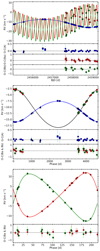 |
Fig. 21. Same as Fig. 19, but for GJ 4383. |
| In the text | |
|
Fig. 22. GLS periodogram of the SWASP photometry of GJ 4383. The horizontal dotted line indicates the corresponding 0.1% FAP level. |
| In the text | |
|
Fig. 23. Mass ratio as a function of the orbital period of the multiple systems characterised in this work and in Baroch et al. (2018), colour-coded by the pEW(Hα). The circular, triangular, and square symbols correspond to SB1, SB2, and ST3 systems, respectively. The upward arrows indicate the mass ratio limits for the systems for which only upper and lower bounds to the secondary masses could be given. The outer and inner orbits of the ST3 are plotted as individual binaries, with the same pEW(Hα). |
| In the text | |
Current usage metrics show cumulative count of Article Views (full-text article views including HTML views, PDF and ePub downloads, according to the available data) and Abstracts Views on Vision4Press platform.
Data correspond to usage on the plateform after 2015. The current usage metrics is available 48-96 hours after online publication and is updated daily on week days.
Initial download of the metrics may take a while.