| Issue |
A&A
Volume 653, September 2021
|
|
|---|---|---|
| Article Number | A173 | |
| Number of page(s) | 15 | |
| Section | Planets and planetary systems | |
| DOI | https://doi.org/10.1051/0004-6361/202140892 | |
| Published online | 30 September 2021 | |
CHEOPS precision phase curve of the Super-Earth 55 Cancri e★
1
Center for Space and Habitability,
Gesellsschaftstrasse 6,
3012
Bern, Switzerland
e-mail: This email address is being protected from spambots. You need JavaScript enabled to view it.
2
Astrobiology Research Unit, Université de Liège,
Allée du 6 Août 19C,
4000
Liège, Belgium
3
Space sciences, Technologies and Astrophysics Research (STAR) Institute, Université de Liège,
Allée du 6 Août 19C,
4000
Liège, Belgium
4
Observatoire Astronomique de l’Université de Genève,
Chemin Pegasi 51,
Versoix, Switzerland
5
Department of Astronomy, Stockholm University, AlbaNova University Center,
10691
Stockholm, Sweden
6
Centre for Exoplanet Science, SUPA School of Physics and Astronomy, University of St Andrews,
North Haugh,
St Andrews
KY16 9SS, UK
7
Physikalisches Institut, University of Bern,
Gesellsschaftstrasse 6,
3012
Bern, Switzerland
8
Aix Marseille Univ, CNRS, CNES, LAM,
Marseille, France
9
Instituto de Astrofísica de Canarias,
38200
La Laguna,
Tenerife, Spain
10
Departamento de Astrofísica, Universidad de La Laguna,
38206
La Laguna,
Tenerife, Spain
11
Institut de Ciències de l’Espai (ICE, CSIC),
Campus UAB, Can Magrans s/n,
08193
Bellaterra, Spain
12
Institut d’Estudis Espacials de Catalunya (IEEC),
08034
Barcelona, Spain
13
Depto. de Astrofísica, Centro de Astrobiologia (CSIC-INTA), ESAC campus,
28692
Villanueva de la Cãda (Madrid), Spain
14
Instituto de Astrofísica e Ciências do Espaço, Universidade do Porto,
CAUP, Rua das Estrelas,
4150-762
Porto, Portugal
15
Departamento de Física e Astronomia, Faculdade de Ciências, Universidade do Porto, Rua do Campo Alegre,
4169-007
Porto, Portugal
16
Space Research Institute, Austrian Academy of Sciences,
Schmiedlstrasse 6,
8042
Graz, Austria
17
Université Grenoble Alpes, CNRS, IPAG,
38000
Grenoble, France
18
Admatis,
Miskok, Hungary
19
Institute of Planetary Research, German Aerospace Center (DLR),
Rutherfordstrasse 2,
12489
Berlin, Germany
20
Université de Paris, Institut de physique du globe de Paris, CNRS,
75005
Paris, France
21
Lund Observatory, Dept. of Astronomy and Theoretical Physics, Lund University,
Box 43,
22100
Lund, Sweden
22
Leiden Observatory, University of Leiden,
PO Box 9513,
2300
RA Leiden, The Netherlands
23
Department of Space, Earth and Environment, Chalmers University of Technology, Onsala Space Observatory,
43992
Onsala, Sweden
24
Dipartimento di Fisica, Università degli Studi di Torino,
via Pietro Giuria 1,
10125,
Torino, Italy
25
Center for Astronomy and Astrophysics, Technical University Berlin,
Hardenberstrasse 36,
10623
Berlin, Germany
26
University of Vienna, Department of Astrophysics,
Türkenschanzstrasse 17,
1180
Vienna, Austria
27
Konkoly Observatory, Research Centre for Astronomy and Earth Sciences,
1121
Budapest,
Konkoly Thege Miklós út 15-17, Hungary
28
IMCCE, UMR8028 CNRS, Observatoire de Paris, PSL Univ., Sorbonne Univ.,
77 av. Denfert-Rochereau,
75014
Paris, France
29
Institut d’astrophysique de Paris, UMR7095 CNRS, Université Pierre & Marie Curie,
98bis blvd. Arago,
75014
Paris, France
30
INAF, Osservatorio Astronomico di Padova,
Vicolo dell’Osservatorio 5,
35122
Padova, Italy
31
Astrophysics Group, Keele University,
Staffordshire,
ST5 5BG, UK
32
Department of Astrophysics, University of Vienna,
Tuerkenschanzstrasse 17,
1180
Vienna, Austria
33
INAF, Osservatorio Astrofisico di Catania,
Via S. Sofia 78,
95123
Catania, Italy
34
Institute of Optical Sensor Systems, German Aerospace Center (DLR),
Rutherfordstrasse 2,
12489
Berlin, Germany
35
Dipartimento di Fisica e Astronomia “Galileo Galilei”, Università degli Studi di Padova,
Vicolo dell’Osservatorio 3,
35122
Padova, Italy
36
Department of Physics, University of Warwick,
Gibbet Hill Road,
Coventry
CV4 7AL, UK
37
Cavendish Laboratory, JJ Thomson Avenue,
Cambridge
CB3 0HE, UK
38
ESTEC, European Space Agency,
2201AZ,
Noordwijk, The Netherlands
39
Institut für Geologische Wissenschaften, Freie Universität Berlin,
12249
Berlin, Germany
40
ELTE Eötvös Loránd University, Gothard Astrophysical Observatory,
9700
Szombathely,
Szent Imre h. u. 112, Hungary
41
MTA-ELTE Exoplanet Research Group,
9700
Szombathely,
Szent Imre h. u. 112, Hungary
42
Institute of Astronomy, University of Cambridge,
Madingley Road,
Cambridge,
CB3 0HA, UK
43
Ingenieurbüro Ulmer – Technische Informatik,
Im Technologiepark 1,
15236
Frankfurt, Germany
44
Airbus
DS Spain
45
Science and Operations Department – Science Division (SCI-SC), Directorate of Science, European Space Agency (ESA), European Space Research and Technology Centre (ESTEC), The Netherlands
46
ELTE Eötvös Loránd University, Institute of Physics,
Pázmány Péter sétány 1/A,
1117
Budapest, Hungary
47
Sydney Institute for Astronomy, School of Physics A29, University of Sydney,
NSW
2006, Australia
48
Division Technique INSU, BP 330,
83507
La Seyne cedex, France
Received:
26
March
2021
Accepted:
11
June
2021
Abstract
Context. 55 Cnc e is a transiting super-Earth (radius 1.88 R⊕ and mass 8 M⊕) orbiting a G8V host star on a 17-h orbit. Spitzer observations of the planet’s phase curve at 4.5 μm revealed a time-varying occultation depth, and MOST optical observations are consistent with a time-varying phase curve amplitude and phase offset of maximum light. Both broadband and high-resolution spectroscopic analyses are consistent with either a high mean molecular weight atmosphere or no atmosphere for planet e. A long-term photometric monitoring campaign on an independent optical telescope is needed to probe the variability in this system.
Aims. We seek to measure the phase variations of 55 Cnc e with a broadband optical filter with the 30 cm effective aperture space telescope CHEOPS and explore how the precision photometry narrows down the range of possible scenarios.
Methods. We observed 55 Cnc for 1.6 orbital phases in March of 2020. We designed a phase curve detrending toolkit for CHEOPS photometry which allowed us to study the underlying flux variations in the 55 Cnc system.
Results. We detected a phase variation with a full-amplitude of 72 ± 7 ppm, but did not detect a significant secondary eclipse of the planet. The shape of the phase variation resembles that of a piecewise-Lambertian; however, the non-detection of the planetary secondary eclipse, and the large amplitude of the variations exclude reflection from the planetary surface as a possible origin of the observed phase variations. They are also likely incompatible with magnetospheric interactions between the star and planet, but may imply that circumplanetary or circumstellar material modulate the flux of the system.
Conclusions. This year, further precision photometry of 55 Cnc from CHEOPS will measure variations in the phase curve amplitude and shape over time.
Key words: techniques: photometric / methods: observational / planets and satellites: atmospheres / stars: individual: 55 Cnc / planets and satellites: individual: 55 Cnc e / instrumentation: photometers
Photometric data are only available at the CDS via anonymous ftp to cdsarc.u-strasbg.fr (130.79.128.5) or via http://cdsarc.u-strasbg.fr/viz-bin/cat/J/A+A/653/A173
© ESO 2021
1 Introduction
55 Cnc e is perhaps the rocky planet most amenable to characterization with CHEOPS. This super-Earth with a radius of 1.88 R⊕ and a mass of 8 M⊕ orbits a very bright (V = 6) G8V host star (Demory et al. 2011; Bourrier et al. 2018a). The planet was initially detected with an apparent 2.8-day orbital period (McArthur et al. 2004; Fischer et al. 2008); this was later revised to the 17-h period (Dawson & Fabrycky 2010) which enabled the detection of the transit in the following year (Winn et al. 2011).
There is evidence for two distinct plausible climatic scenarios for 55 Cnc e: either it is a lava world without a significant atmosphere (Demory et al. 2016a), or it has a very thick atmosphere (Angelo & Hu 2017; Bourrier et al. 2018a). Existing transit observations of 55 Cnc e at 3.6 and 4.5 μm show similar transit depths, also consistent with an opaque atmosphere or no atmosphere. Mahapatra et al. (2017) studied cloud properties and found that mineral clouds could form in a thick atmosphere scenario for 55 Cnc e.
Ultra-short period rocky planets may not have been born that way. A growing body of evidence suggests that some ultra-short period planets may have once been giants that lost most of their gaseous envelopes due to photoevaporation (Lecavelier des Etangs et al. 2004; Owen & Wu 2017; Fulton et al. 2017; Van Eylen et al. 2018). 55 Cnc e may represent one end-point of planetary evolution under high irradiation.
Though the planet’s density is consistent with a purely rocky composition (Madhusudhan et al. 2012; Dorn et al. 2017), its Spitzer 4.5 μm phase curve peaks prior to the secondary eclipse, and this indicates a large day-night temperature contrast (Demory et al. 2016a). However, Kite et al. (2016), Hammond & Pierrehumbert (2017) and Angelo & Hu (2017) argue that the 4.5 μm phase curve indicates that the day-to-night side heat redistribution is too efficient to be explained by heat transport due to currents in a molten lava ocean. They suggest that the 4.5 μm phase curve observations may instead require the presence of a thick atmosphere with a pressure ≳ 1.4 bar and a temperature of 2400 K at the photosphere. Recent work by Zilinskas et al. (2020) shows that JWST and Ariel may be able to distinguish between the plausible atmosphere scenarios, and Jindal et al. (2020) and Deibert et al. (2021) rule out low mean molecular weight atmospheres.
Recently, Sulis et al. (2019) used MOST photometry to measure variability in the phase curve of 55 Cnc e; the amplitude and phase of maximum light are seen to vary from year to year from 113 to 28 ppm and from 5° to 217°. The authors were not able to identify a single origin of this variability. Different scenarios were proposed, including the following: star-planet interactions, the presence of a transiting circumstellar torus of dust, or an instrumental artifact.
The secondary eclipse depth of the planet at 4.5 μm varied by a factor of three between 2012 and 2013 (Demory et al. 2016b; Tamburo et al. 2018). The corresponding thermal emission from the dayside atmosphere must have varied by ~ 1500 K between the two epochs, which could be explained by atmospheric albedo variability, or large-scale surface volcanic activity, for example, like the volcanic plumes observed on Jupiter’s moon Io (e.g. Spencer et al. 1997; McEwen et al. 1998). These dynamic features were detected at 4σ significance (Demory et al. 2016b). The secondary eclipse was not detected with MOST (Sulis et al. 2019), and a weak 3σ secondary eclipse has been claimed from TESS observations (Kipping & Jansen 2020).
Previous observations support the presence of an atmosphere with a lack of H2O and a hint of HCN (Tsiaras et al. 2016; Esteves et al. 2017), despite the lack of H detection by Ehrenreich et al. (2012). It is possible that an H2-rich atmosphere could be present without a detection of H, as the H may get swept away by radiation pressure. However the lack of Ly-α and helium absorption from 55 Cnc e may point to a lack of a thick modern atmosphere (Zhang et al. 2021). This alternatively may imply a C/O ratio greater than solar (Madhusudhan et al. 2012). In this regime, carbon- and nitrogen-based molecules such as HCN, N2 and CO are expected to be the trace gasses in the atmosphere (Venot et al. 2015; Miguel 2019). In such an environment, one might also expect CH4, C2H2, and others to be detected (Heng & Tsai 2016). The Spitzer 4.5 μm transits, however, yield a radius consistent with optical and near-IR observations, implying a flat transmission spectrum (Demory et al. 2016b).
Stellar magnetic activity is also a possible culprit in the apparent phase variations. The rotation period of the star is approximately 40 days (Henry et al. 2000; Fischer et al. 2008). Folsom et al. (2020) mapped the large-scale magnetic field of 55 Cnc and find a 5.8 G dipole, tilted with respect to the rotation axis. Simulations of the stellar wind predict that planet e orbits inside the Alfvén radius, so the planet’s influence on the stellar wind propagates back to the stellar surface. This could result in star-planet interactions. On long timescales, Bourrier et al. (2018a) used photometric and spectroscopic observations to constrain the magnetic activity cycle of the host star Pcyc = 10.47 ± 0.21 yr. Spectroscopic observations on the order of weeks may be required to constrain the relevant timescales for stellar magnetic activity. Far-UV observations of 55 Cnc with HST also showed chromospheric variability at many timescales, which may be linked to star-planet interactions as well (Bourrier et al. 2018b).
In this work, we aim to probe the following with CHEOPS photometry: (1) if reflected light is a plausible source of the photometricvariability, (2) if stellar variability on the orbital period of the planet is an equally compatible source, (3) what is the limiting precision of CHEOPS photometry for bright stars, and (4) if we detect a significant secondary eclipse in the optical. In Sect. 2, we give background on the CHEOPS telescope and mission design, and the details of the observations presented inthis work. In Sect. 3, we outline methods for mitigating systematics in CHEOPS observations like those of 55 Cnc e. In Sect. 4, we devise a photometric model for the detrended CHEOPS photometry of 55 Cnc e. We discuss the interpretation of the results in Sect. 6 and conclude in Sect. 7.
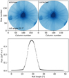 |
Fig. 1 Smear contamination correction. Top-left: an example CHEOPS exposure where the smear contamination from 53 Cnc, located outside the subarray image, is visible at the left of 55 Cnc (the star at the center of the field of view). Top-right: the same frame after the DRP v12 smear correction. Bottom: the estimated smear contamination flux within the DEFAULT aperture as a function of the observation roll angle which affects each orbit. |
2 CHEOPS
2.1 Background
CHEOPS is an on-axis Ritchey-Chrétien telescope with a 320 mm diameter primary mirror (Benz et al. 2021), optimized for high-precision photometry (Lendl et al. 2020). The primary mirror is partially obscured by the secondary mirror, which is held in place by three supports. The telescope is intentionally defocused, and due to the secondary mirror supports, CHEOPS exposures have a distinctive three-pointed point-spread function (PSF; see Fig. 1), with its core spanning 32 pixels across.
The spacecraft is nadir-locked in a low-Earth orbit about 700 km from the Earth’s surface, which causes stars in the field of view to rotate around the line of sight once per CHEOPS orbit. Neighboringstars can introduce periodic photometric systematics, that we will discuss in Sect. 3.2.
The CHEOPS spacecraft always points its backside toward the Sun, and variable spacecraft heating may occur when slewing between targets. Earth occultations of the target star also cause temperature perturbations in the telescope optical assembly. We discuss mitigation for temperature variations during a measurement in Sect. 3.3.
CHEOPS exposures are recorded by a back-illuminated, frame-transfer CCD, which spans a broad, optical bandpass similar to the Gaia G filter. Exposures less than 23 s in duration are stacked on-board to save downlink bandwidth (the image downlink cadence varies between 23 and 60 s depending on the exposure time). However, before stacking, “imagettes” of 30 pixels in radius are extracted. These small images are centered in the CHEOPS field of view and contain the PSF of the target star. In the case of the 55 Cnc observations, imagettes were stacked in pairs before being downlinked to the ground. As a result of these frequent reads (the cadence of each stacked imagette is 4.4 s) and the well-resolved PSF of CHEOPS, it is possible to do precise PSF photometry on the target star – we discuss insights on the 55 Cnc e photometry from PSF photometry in Sect. 3.4.
CHEOPS observation logs, corresponding to the IOC observations in the first row and the phase curve observations in the second row.
2.2 Observations
A single primary transit of 55 Cnc e was observed during the CHEOPS In-Orbit Commissioning (IOC) phase on UT 2020 March 09. Due to the brightness of the target, an effective exposure time of 30.8 s was achieved by the stacking of 14 individual readouts of 2.2 s. Imagettes were stacked on board in pairs, which means that with a cadence of 30.8 s seconds a stacked image and seven stacked imagettes were downlinked. CHEOPS also observed 1.6 orbital phases of 55 Cnc over 26 hours on UT 2020 March 23–24, stacking 20 × 2.2 s individual frames and thus obtaining a final 44.5 s cadence. The log of the observations is presented in Table 1. Gaps in the observations correspond to occultations of the target by the Earth, and passes by the spacecraft through the South Atlantic Anomaly, during which images are discarded as there is a significantly increase in the cosmic ray hits.
The observations were automatically reduced by the CHEOPS Data Reduction Pipeline (DRP v12, Hoyer et al. 2020). The DRP takes the raw images from the spacecraft and produces time-series photometry of the target star for analysis by the user. The DRP produces four light curve data products for each visit, called the “DEFAULT, RSUP, RINF” and “OPTIMAL” apertures. In the following analysis, we focus on the “DEFAULT” aperture product with a circular aperture of 25 pixels in radius.
3 Mitigating CHEOPS Spacecraft Systematics
The design of the CHEOPS spacecraft introduces several systematics to precision photometry which we seek to outline and account for below.
3.1 Pointing
The spacecraft pointing is generally better than 1′′, where 1′′ spans about one pixel (Benz et al. 2021). However, the exposures that occur just before and after Earth occultation are often more likely to show significant pointing offsets – see Fig. 2d. We mask out all photometry with centroids > 3.5σ away from the median centroid.
3.2 Roll angle
Due to the nadir-locked orientation of CHEOPS, the field of view of the telescope rotates once per CHEOPS orbit. In practice, this means that the field stars rotate about the target star. The core of the PSF is 32 pixels across, but it has extended wings out to ~ 50 pixels. The extended and irregular shape of the CHEOPS PSF and the rotation of the field, leads to variations in the flux inside the photometricaperture which is centered on the target star. The sky background flux is also a strong function of the position of CHEOPS inits orbit, as background light from Earthshine contaminates the aperture close to Earth occultation. While these sources of contamination are present in all CHEOPS observations, in the case of 55 Cnc they do not play a major role due to the brightness of the star. However, decorrelating the flux of the target star against the roll angle of the spacecraft is necessary to ensure the rotating field does not introduce correlated noise in the photometry.
Smearing
CHEOPS has no shutter to block the incoming light between one exposure and the next. This means that light continues to be collected during the frame transfer from the exposed section to the covered, read-out section. It takes 25 ms to transfer the full CCD image area (1024 pixel-rows) to the covered section for read-out. Therefore, a consequence of this constant transfer speed is the presenceof “smearing trails” in the images. Smearing trails are vertical stripes of flux going through every PSF in an image. All stars in the CHEOPS field of view (full CCD) leave a smearing trail after each exposure. Because the transfer time is constant, that is independent of the exposure time and the stellar brightness, smear trails are stronger for brighter stars. Therefore, while in most of the cases they are hard to detect, the flux level of the trails becomes significant when the target star or a neighbor star is very bright. It is important to make the distinction between the self-smear trail of the target star and the smearing trails from the field stars. The smearing trail of the target star is always “fixed” in the image, only following the small jitter of the target. The photon noise is negligible and it has no impact in the photometry as it almost does not change during the whole visit. However, things are much more complex with the smearing trails of the field stars. As the neighboring stars rotate around the target, the vertical smearing trails sweep back and forth over the target star (on the horizontal axis), producing a highly predictable positive flux anomaly in uncorrected photometric extractions. Any star in the field of view (within a radius of 17 arcmin) may contaminate the photometric aperture with its smearing trails at least once per orbit. Figure 1 top-left and bottom illustrate the problem in the case of 55 Cnc and the bright neighbor 53 Cnc (Gaia G magnitude 5.17).
As of DRP v12 (Hoyer et al. 2020), the effect of smearing is removed from each subarray frame before photometry is computed (see Fig. 1 top-right). This is accomplished by forward modeling the smearing produced by each star in CHEOPS CCD, except for the target, to estimate the flux deviations due to the smearing. Finally, this estimated smear signal is directly subtracted from each subarray frame. No further smear corrections are needed in the photometric analysis that follows – see Fig. 2e.
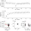 |
Fig. 2 Photometry from CHEOPS of 55 Cnc e and detrending vectors. (a) Raw fluxes returned by the Data Reduction Pipeline (DRP) aperture photometry observations over the 1.6 orbital phases of 55 Cnc e, centered on a transit. Red points are centroid outliers and are masked from analysis. The gaps in the observations occur primarily when Earth is occulting the target star. The horizontal dashed line at flux unity represents the median flux, about which we see variations in flux in the phase curve. (b) One component of the variations in the raw phase curve in panel a is a “ramp” feature which is anticorrelated with the telescope tube temperature, denoted the “ThermFront 2 Sensor” temperature. A full discussion of the link between the flux variations and telescope tube temperature is written in Sect. 3.3. The temperature of the telescope tube rises asymptotically from a minimum at the beginning of the observations to a near-constant value after ~ 0.5 days. There is an additional perturbation in the temperature once per orbit, thought to be caused by illumination of the telescope optical assembly by the Earth during occultation. (c) Changes in the DRP flux are associated with changes in the ThermFront 2 Sensor temperature after dividing out the transit with a slope of − 193 ± 10 ppm/degree Celsius. (d)Measured centroid of the target star on the detector in pixel units – outliers in red are masked from further analysis. (e) Trends in DRP flux with roll angle after correction for smearing (see Sect. 3.2) are ≲ 100 ppm, and are a result of correlations between the spacecraft roll angle and the contamination from nearby stars, and in the background light (see Sect. 3.2). Red points are the masked centroid outliers, which mostly occur immediately before and after the Earth occultation. |
3.3 The “Ramp”
Space-based photometry is often affected by systematic variations in the measured flux from quiescent target stars, sometimes called “ramps”. Ramps have been observed in photometry from the Hubble Space Telescope (HST) WFC3 (e.g., Berta et al. 2012; Zhou et al. 2017; Stevenson & Eck 2019), HST/STIS (Demory et al. 2015), and Spitzer/IRAC (e.g., Deming et al. 2006; Deming 2009; Désert et al. 2009; Knutson et al. 2008; Demory et al. 2011). Charge trapping is one proposed mechanism for producing the observed ramps in WFC3 and IRAC photometry (e.g.: Agol et al. 2010; Zhou et al. 2017).
A ramp feature has been observed in CHEOPS photometry on some targets including 55 Cnc – see Fig. 2a. The amplitude of the ramp feature in the 55 Cnc e phase curve time series is ~ 100 ppm, showing a decrease in the apparent flux of the target star over a span of ~ 0.5 days at the beginning of the visit. The ramp effect has been observed on other targets as well, sometimes as an asymptotically increasing flux trend, and sometimes as a decreasing one.
Our current best hypothesis for the cause of the ramp feature in CHEOPS photometry is solar thermal forcing of the telescope optical assembly. The scale of the PSF has been noted to vary slightly with time, most sharply at the beginning of a time series, and settles to a constant scale factor after several hours (more on PSF photometry in Sect. 3.4). The changing scale of the PSF could be due to small differences in the distance between the primary and secondary mirrors as a result of temperature changes in the telescope tube as the solar illumination on the spacecraft varies between pointings. The change in PSF scale with time may modulate the flux which falls within fixed apertures, causing the apparent ramps in flux.
If the observed flux ramp is the result of changes in the PSF scale caused by thermal settling of the spacecraft, then we can remove the ramp by detrending against the temperature of the telescope tube – see Fig. 2c. The telescope temperature is recorded in the housekeeping time series from the spacecraft, shown in Fig. 2b. We include this temperature time series as a basis vector in the detrending analysis in Sect. 4, which removes the − 193 ± 10 ppm variation in flux per degree Celsius in the DRP photometry.
3.4 Insights from PSF photometry
The defocused PSF is sampled over ~32 pixels, allowing us to build up a precise PSF model which can be fit to each exposure via PIPE: the PSF Imagette Photometric Extraction pipeline. PSF photometry has a few distinct benefits for validating detections made with the standard DRP (aperture) photometry,since PSF photometry: (1) is resilient against cosmic ray strikes, bad pixels, and detector artifacts such as smearing, because it fits a model to the whole of the PSF rather than simply summing within an aperture, (2) explicitly accounts for changes in the scale of the PSF as a function of time, and (3) gives access to the subexposures that make up each exposure stack, and thus has finer time sampling than DRP photometry. We enumerate details on the PSF photometric extraction in Appendix B, including a direct comparison of the DRP and PSF photometry in Fig. B.5. There are a few challenges associated with PSF photometry which affect DRP photometry to a lesser extent, including for example measuring the background from the small imagettes and source blurring due to pointing jitter during the exposure, so we present results with both the DRP and PSF photometry in this work.
4 Detrended CHEOPS Photometry of 55 Cnc
In this section, we aim to measure the shape and amplitude of the variations in flux of the 55 Cnc system while simultaneously accounting for: the systematics which affect the photometry, the transit, and any evidence of planetary occultations.
In Sect. 4.1, we select a small set of basis vectors which we use to detrend the light curve. In Sect. 4.2, we detail the model used to fit the two transits. We outline a series of models for the observed phase variations in Sect. 4.3, each with the same set of basis vectors but with a unique, physically-motivated phase variation model. We measure the weights and uncertainties on each set of basis vectors and the phase variation model with the No U-Turn Sampler (NUTS) implemented by PyMC3 (Salvatier et al. 2016b), and compare the predictive power of each model with Leave-One-Out Cross-Validation (LOO-CV; Vehtari et al. 2017).
4.1 Detrending basis vectors
We detrend the light curve against a set of basis vectors which are correlated with the flux of 55 Cnc. There are many “housekeeping” sensor readouts, as well as photometric by-products like target centroids and background levels, which are packaged in the DRP data products as time series along with the times and fluxes.
We performed an exhaustive search through these candidate detrending basis vectors to identify which vectors yield the most significant improvements to the light curve fits without overfitting. We quantify the improvement of each candidate basis vector in the detrended light curve with the Bayesian Information Criterion (BIC), and find that a combination of four basis vectors produce the minimum (ideal) BIC. These four vectors are: the cosine and sine of the spacecraft roll angle (see description of roll angle in Sect. 3.2), the ThermFront 2 thermistor readout which tracks the telescope temperature (see description in Sect. 3.3), and a unit vector. The unit vector accounts for the constant mean flux of the star. Adding further basis vectors such as the PSF centroid or higher order functions of the earlier basis vectors are disfavored by the BIC.
4.2 Transit and eclipse
We simultaneously fit the two transits of 55 Cnc e along with the detrending basis vectors and the phase curve models with an Agol et al. (2020) transit model assuming the period from Bourrier et al. (2018a), and the interferometric stellar radius and derived mass by von Braun et al. (2011). We fit for quadratic limb-darkening parameters using the efficient triangular sampling method of Kipping (2013). The secondary eclipse of the planet is fixed in time to occur at the expected eclipse time for zero eccentricity, consistent with the small or zero eccentricity found by Bourrier et al. (2018a).
4.3 Phase variation models
Several physically-motivated models could be applied to the out-of-transit phase variability of the 55 Cnc e system. We use: a Lambertian model, which naturally occurs when a planet emits or scatters light isotropically; the piecewise-Lambertian model of Hu et al. (2015), which describes a planetary surface that behaves like a Lambertian sphere between two longitudes; a simple sinusoidal model which assumes the flux is varying with the period of the planet and an arbitrary phase offset. We detail the sampling procedure in Sect. 4.4 and compare the model fits in Sect. 4.5.
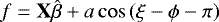
In each following section outlining a phase curve model, we describe the baseline model as:
 (1)
(1)
which is the best-fit weights  to the linear combination of basis vectors in the design matrix X, which is composed of the following column vectors: the cosine and sine of the roll angle, a unit vector, and the “ThermFront 2” sensor temperature.
 |
Fig. 3 Select posterior distributions for key parameters in the composite transit, eclipse and piecewise-Lambertian phase curve model. The parameters are the planet radius Rp, impact parameteter b, full amplitude of the phase variations, and the start and stop longitudes of the piecewise-Lambertian model ξ1, ξ2. The full posterior distribution correlation matrix is given in Appendix A. |
4.3.1 Sinusoidal model
The simplest model to describe the phase variations of the 55 Cnc e system is simply cosine-shaped variability with a fixed period set to the planet’s orbital period,
 (2)
(2)
where ξ is the orbital phase, which is defined on [−π, π] where |ξ| = π is the time of transit and ξ = 0 is the secondary eclipse. We fit for the amplitude a, phase offset ϕ.
We do not assume that the origin of the sinusoidal signal is the planet, which would imply that the eclipse depth should be equivalent to the amplitude of the sinusoid at the mid-eclipse time, and the in-eclipse fluxes would be constant. As a result, our simple model changes in flux during the time of the expected secondary eclipse, and the eclipse depth is an unconstrained free parameter.
4.3.2 Lambertian model
A Lambertian sphere isotropically scatters or emits thermally, giving a phase function:
 (3)
(3)
Here the phase function is modulated by an amplitude parameter a and an eclipse function E which is the eclipse model with no limb darkening, which models the eclipse of the planet. By construction, this model has no phase offset.
4.3.3 Piecewise-Lambertian model
Appendix A of Hu et al. (2015) defines a piecewise-Lambertian sphere for describing the Kepler optical phase curve of the apparently asymmetric planet Kepler-7 b. The model is constructed with significant reflection or emission between two longitudes, and negligible reflection and emission elsewhere. We implement the Hu et al. (2015) model to test if an asymmetric planetary albedo distribution could explain the apparently asymmetric phase variations of 55 Cnc e. This model incurs two additional fitting parameters corresponding to the longitudes ξ1, ξ2 which bound the less reflective hemisphere.
4.4 Posterior sampling
For each of these models, we sample the posterior distributions for the transit parameters, the  best-fit estimators, as well as the parameters relevant to each phase curve model, using the No U-Turn Sampler (NUTS) implemented by PyMC3 (Salvatier et al. 2016b). The NUTS is a variant of Hamiltonian Monte Carlo, which is a gradient-based Monte Carlo approach that has been shown to be computationally efficient for sampling posterior distributions for high-dimensional problems (see e.g. Betancourt 2017).
We also introduced the flux uncertainty on each photometric measurement as a free parameter, and introduce a term to the likelihood that penalizes larger uncertainties. This has the effect of finding the smallest uncertainties that bring the reduced χ2 to unity. The maximum-likelihood solution has a uncertainty per flux of 84 ± 3 ppm, which is larger than the DRP estimated flux uncertainty of 51 ppm. Figure 3 shows posterior distributions for some key parameters, and the full joint posterior correlation matrix is shown in Appendix A.
4.5 Model comparison
We measure the relative likelihood that each model describes the observations while penalizing the models with more free parameters with Leave-One-Out Cross-Validation statistic and the Widely Applicable Information Criterion (LOO-CV and WAIC; Vehtari et al. 2017). Both techniques are a computational efficient method for estimating the relative likelihood that one model in a set is preferred over the others, using only the posterior samples from the precomputed Markov chains used for parameter inference. The preferred models have the smallest ΔLOO or ΔWAIC, where moresignificant preferences for a given model have, for example, ΔLOO > 10. The results are given in Table 2; the piecewise-Lambertian model is the preferred model, followed closely by the sinusoidal model, and finally the symmetric Lambertian model. We adopt the physically-motivated piecewise-Lambertian model as the most likely in the following discussion, noting that the empirical sinusoidal model fits about as well as the piecewise-Lambertian.
Change in the Leave-One-Out Cross-Validation and Widely Applicable Information Criterion statistics between models compared with the best-fitting model, which is the piecewise-Lambertian model of Hu et al. (2015).
5 Results
Figure 4 shows the best-fit transit and Piecewise-Lambertian model, and the parameters are listed in Table 3. The ratio of radii Rp∕R⋆ and impact parameter b are consistent with the Spitzer observations by Demory et al. (2016b). Figure 5 shows a comparison between the models considered for the phase variations.
The maximum-likelihood eclipse depth is  ppm, or 2.2σ consistent with zero eclipse depth. This is consistent with the Kipping & Jansen (2020) claim of TESS occultation of depth 15.0 ± 4.8 ppm.
Comparison with PSF photometry
The analysis described above was conducted on the Data Reduction Pipeline (DRP) photometric products. To validate the results from DRP photometry, we also reduce and analyze PSF photometry constructed from the imagettes. The PSF photometric extraction issummarized in Appendix B.
We analyze the PSF photometry with the same procedure as outlined above for the DRP photometry. The differences in the two analyses include: (1) the detrending basis vectors for the PSF photometry include two principal components of the PSF shape changes in place of the ThermFront 2 vector (details in Appendix B); (2) the photometric cadence is shorter because photometry is extracted from the imagettes; (3) a smaller fraction of the total number of exposures is rejected due to the finer time sampling.
The same sequence of models is fit to the PSF photometry and we verify that the PSF photometry produces consistent (within 1-σ) measurements for each of the physical parameters in Table 3. This validation step strengthens the claim that the flux variations are indeed astrophysical and their interpretation is robust against different photometric extraction techniques.
6 Discussion
Combining the optical CHEOPS observations with the existing optical and infrared observations creates a difficult puzzle. The CHEOPS optical light curves confirm that the flux variations may be variable in time, as suggested by the mismatch in phase and amplitude with the MOST observations of Sulis et al. (2019, see also Appendix C). CHEOPS is scheduled to observe 55 Cnc e again, and the exquisite photometric precision demonstrated by CHEOPS on the single phase curve observation presented here suggests that we verify the amplitude and timescales of the flux variations in the system. We have shown that CHEOPS can achieve sufficient precision to search for variability in the phase variations in the 55 Cnc system from one phase to the next, due to the exceptionally high-precision optical photometry from CHEOPS.
In the following subsections, we enumerate a series of mysteries left in the 55 Cnc system which future CHEOPS observations can interrogate.
6.1 Planetary reflection
In principle, the maximum-likelihood eclipse depth of 20 ± 8 ppm constrains the geometric albedo of the planet, which can be defined as:
 (4)
(4)
if we neglect thermal emission in the CHEOPS bandpass. In practice however, the 1σ upper limit on the eclipse depth yields an uninformative upper limit on the geometric albedo Ag < 0.98.
6.2 Optical secondary eclipse
The significant eclipse detected in the infrared and the lack of a clear eclipse in the optical presents another puzzle. The interpretation that the infrared eclipse is due to planetary light being occulted by the host star is challenged by the fact that the eclipse depth changed from one observation to the next, requiring the planet to change in size, albedo, thermal emission, or some combinationof the three. Future observations will eventually measure any variability in the transit depth in the optical, which constrains the first scenario. Albedo variations could be detected by CHEOPS as variations in the optical eclipse depth, and will require further observation. The thermal emission could be further tested with large space-based infrared observatories.
The phase variation model with the maximum predictive power is the piecewise-Lambertian model of Hu et al. (2015) which describes anasymmetric albedo distribution on the planet. For self-consistency with this model, we have chosen to fix the eclipse depth to be equivalent to the full-amplitude of the phase variations at the mid-eclipse time. This could affect the Monte Carlo results in the following way: attempting to fit the significant phase variations with a high albedo will produce a strong secondary eclipse which is not observed, so the fit will negotiate a compromise between significant phase variations and an insignificant secondary eclipse.
6.3 Properties of circumstellar or circumplanetary material
Another hypothesis based on Demory et al. (2016b) states the planet is surrounded by material that is opaque in the optical but transparent in the infrared. Clumps of material could cause the variable flux modulation observed in the optical. This could occur if the circumstellar or circumplanetary dust has a narrow range of particle sizes. Let the radius of the particle be r, the wavelength be λ and x = 2πr∕λ. For CHEOPS, x ≳ 1 implies r ≳ 0.1μm. For 4.5 μm Spitzer, x ≲ 1 implies r ≲ 0.7μm. Collectively, the plausible range of particle radii is 0.1 ≲ r ≲ 0.7μm.
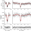 |
Fig. 4 Detrended CHEOPS photometry of 55 Cnc e. Upper: the Data Reduction Pipeline (DRP) aperture photometry fluxes in black, and in red the best-fit linear combination of a transit model, a piecewise-Lambertian phase variation, and several detrending vectors. This fit is used to infer the best-fit transit parameters. The left column shows transit observations obtained during the in-orbit commissioning (IOC) phase, and the right column shows the phase curve observation. Middle: the residuals after the instrumental and systematic variations have been removed (black) and several draws from the posterior distributions for the transit and phase curve parameters (red). Lower: the residuals after removing allsystematics and astrophysical signals from the observations. |
6.4 Star–planet interactions
Interactions between the stellar and planetary magnetic fields could be responsible for excess flux emitted by the system, which could appear to vary on the orbital timescale of the planetary orbit (see e.g.: Jardine & Collier Cameron 2008). We can use order-of-magnitude estimates for the energy liberated by magnetospheric interactions in the star-planet system with the observed stellar magnetic field properties from Folsom et al. (2020) to estimate if sufficient energy is available to generate the observed phase variations with amplitude ~ 80 ppm. Zarka (2007) gives a simple relation for the power Pd dissipated by unipolar or dipolar satellite-magnetosphere interactions
 (5)
(5)
where ϵ is an unknown efficiency factor of order 0.1, v is the orbital velocity taken from Folsom et al. (2020), B is the local magnetic field at the planet e also from Folsom et al. (2020), and Robs is the obstacle radius which we take as the magnetospheric radius Rm defined in Jardine & Collier Cameron (2008). We express the power dissipated Pd ∕L as a ratio with the luminosity of the star L = 0.582 L⊙ (von Braun et al. 2011), finding Pd∕L ≈ 10−10 for a planetary magnetic field strength of order 1 G. Given that the full-amplitude of the CHEOPS phase variations ~ 80 ppm is five orders of magnitude larger than the energy budget for magnetospheric interactions, unipolar or dipolar interactions likely are not solely responsible for the phase variations in the system.
To further test the star–planet interaction hypothesis, time-resolved simultaneous observations of the phase curve and spectroscopic activity indicators may be necessary. If the star has chromospheric hot spots induced by the planet as imagined by Folsom et al. (2020), those spots may emit excess flux in the CaII H & K lines, which could be observed with ground-based spectroscopy. If the chromospheric activity indeed varies with the orbital phase of the planet, and also varies on longer timescales from one planetary orbit to another, the star–planet interaction model might succinctly explain the flux variations, though no such evidence for line variations was found by Ridden-Harper et al. (2016).
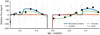 |
Fig. 5 Comparison of the different models tested (colored curves), compared to the best-fit residuals obtained for the sinusoidal model (gray, and binned once per CHEOPS orbit in black). |
Maximum-likelihood parameters for the transit model.
7 Conclusion
CHEOPS observations confirm that the 55 Cnc system varies in flux over the orbital period of planet e. The origin of these flux variations is unclear. Two scenarios ruled unlikely by this work are that the flux variations are the result of reflection from the planet’s surface (observed amplitude is too large and asymmetric), or that magnetospheric interactions are inducing excess emission from the star (observed amplitude is too large). A surviving hypothesis for explaining the optical and infrared observationsis that dust is orbiting either the star or planet, obscuring the secondary eclipse in the optical but not the infrared.
Though the observations of 55 Cnc e may be enigmatic, it is clear that CHEOPS is performing as predicted (Hoyer et al. 2020; Futyan et al. 2020; Deline et al. 2020). We have shown that CHEOPS is a photometrically stable observatory capable of measuring the 71.5 ± 6.5 ppm variability of the 55 Cnc system in a single visit. CHEOPS is currently collecting more high-precision phase curves for 55 Cnc and several other bright exoplanet systems, which will be the subjects of future publications.
Acknowledgements
This manuscript benefited from the feedback provided by an anonymous referee. We gratefully acknowledgethe open source software which made this work possible: astropy (Astropy Collaboration 2013, 2018), ipython (Pérez & Granger 2007), numpy (Harris et al. 2020), scipy (Jones et al. 2001), matplotlib (Hunter 2007), emcee (Foreman-Mackey et al. 2013), batman (Kreidberg 2015), PyMC3 (Salvatier et al. 2016b), arviz (Kumar et al. 2019). This research made use of exoplanet and its dependencies (Agol et al. 2020; Astropy Collaboration 2013, 2018; Foreman-Mackey et al. 2020; Kipping 2013; Luger et al. 2019; Salvatier et al. 2016a; Theano Development Team 2016). This work has been carried out in the framework of the PlanetS National Centre of Competence in Research (NCCR) supported by the Swiss National Science Foundation (SNSF). CHEOPS is an ESA mission in partnership with Switzerland with important contributions to the payload and the ground segment from Austria, Belgium, France, Germany, Hungary, Italy, Portugal, Spain, Sweden, and the United Kingdom. The Swiss participation to CHEOPS has been supported by the Swiss Space Office (SSO) in the framework of the Prodex programme and the Activités Nationales Complémentaires (ANC), the Universities of Bern and Geneva as well as of the NCCR PlanetS and the Swiss National Science Foundation. This work benefited from support from the Swiss National Science Foundation (PP00P2-163967 and PP00P2-190080). This project has received funding from the European Research Council (ERC) under the European Union’s Horizon 2020 research and innovation programme (project FOUR ACES; grant agreement No 724427). This work was supported by FCT – Fundação para a Ciência e a Tecnologia through national funds and by FEDER through COMPETE2020 - Programa Operacional Competitividade e Internacionalização by these grants: UID/FIS/04434/2019; UIDB/04434/2020; UIDP/04434/2020; PTDC/FIS-AST/32113/2017 and POCI-01-0145-FEDER-032113; PTDC/FIS-AST/28953/2017 and POCI-01-0145-FEDER-028953; PTDC/FIS-AST/28987/2017 and POCI-01-0145-FEDER-028987. S.C.C.B. and S.G.S. acknowledge support from FCT through FCT contracts nr. IF/01312/2014/CP1215/CT0004, IF/00028/2014/CP1215/CT0002. O.D.S.D. is supported in the form of work contract (DL 57/2016/CP1364/CT0004) funded by national funds through Fundação para a Ciência e Tecnologia (FCT). X.B., S.C., D.G., M.F. and J.L. acknowledge their roles as ESA-appointed CHEOPS science team members. A.C.C. and T.W. acknowledge support from STFC consolidated grant number ST/R000824/1. This project was supported by the CNES. S.H. gratefully acknowledges CNES funding through the grant 837319. P.M. acknowledges support from STFC consolidated grant number ST/M001040/1. K.G.I. is the ESA CHEOPS Project Scientist and is responsible for the ESA CHEOPS Guest Observers Programme. She does not participate in, or contribute to, the definition of the Guaranteed Time Programme of the CHEOPS mission through which observations described in this paper have been taken, nor to any aspect of target selection for the programme.
Appendix A Posterior distributions
In the corner plot in Fig. A.1, there are two sets of these basis vectors included in the fit, one per CHEOPS visit, corresponding to the In-Orbit Commissioning (IOC) transit observation and the phase curve observation, respectively.
 |
Fig. A.1 Posterior distributions and joint correlations between all free parameters in the joint fit to the In-Orbit Commissioning transit and phase curve observations sampled with the No U-Turn Sampler. The parameters include: the mid-transit time t0, limb-darkening parameters u0, u1, the ratio of planetary to stellar radius Rp∕R⋆, the impact parameter b, the eclipse depth δecl; two sets of detrending vector weights for the following vectors, one per visit: the ThermFront 2 temperature sensor reading, thecosine and sine of the roll angle, and a unit vector; the amplitude of the piecewise-Lambertian variations A; and the startand stop longitudes of the lower-reflectivity region ξ1 and ξ2. The last parameter, log σ is the natural logarithm of the flux uncertainty for each measurement. |
Appendix B PSF photometry
We used both imagettes and subarrays of 55 Cnc to measure how the PSF changes with time by deriving independent PSFs for each of the visit’s 16 CHEOPS orbits. For each exposure, the pixel values were normalized and listed with coordinates relative to the center of the PSF. Each CHEOPS orbit produced about 75 subarray images and 750 imagettes, with centers dithered by a fraction of apixel. The table of pixel values and their relative pixel coordinates was then fit with a 2D-spline with knots located in a grid of thesame resolution as the pixel grid. Sigma-clipping was used to remove deviating pixels (from e.g. cosmic ray hits). To find what parts of the PSF changes with time, a principal component analysis (PCA) was performed on the spline coefficients of the 16 derived PSFs. The four most important components are illustrated in Fig. B.1.
Comparison of the best-fit transit model parameters for the DRP and PSF photometric reductions.
For each imagette, a best-fit PSF was produced by combining the first 10 principal components (named U0 to U9, where U0 is the average PSF). The relative importance of each component can then be followed in time to track PSF changes. Figure B.2 shows how U1 to U8 vary in time, where U1 is clearly dominating the change with time. In this figure any roll angle dependent variation has been removed and the measurement points have been binned by a factor 100. In Fig. B.3, we see the component coefficients as a function of roll angle, where the long-term dependence from Fig. B.2 has been removed and the measurement points again binned by a factor of 100, but this time in roll angle. The roll angle dependence is generally weak, except for U3. The photometric precision improves only slightly by fitting an increasingly accurate PSF. Going from one principal component to 3 only improves the photometric precision by 2.5% as measured by the point-to-point mean absolute deviation. The precision keeps improving slowly another 0.5% until 10 components are used, and decreases slowly after that, likely due to the over-fitting of noise. The main advantage of decomposing the PSF into principal components is thus not necessarily to improve the noise, but to follow how the PSF changes over time and enable correction for long-term trends (in particular the ramp; see Fig. 2).
 |
Fig. B.1 Four principal components with the highest eigenvalues (from the PCA of the PSFs). |
 |
Fig. B.2 Relative coefficients of the U1 to U8 components from the PCA of the PSFs as a function of time. The roll angle dependence has been removed in this plot. |
 |
Fig. B.3 Relative coefficients of the U1 to U8 components from the PCA of the PSFs as a function of roll angle. The long-term time dependence from Fig. B.1 has been removed in this plot, to reduce the scatter and better see the roll angle trend. |
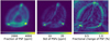 |
Fig. B.4 CHEOPS PSF and its changes over the 55 Cnc e visit. The left panel shows the mean PSF, the central panel shows the standard deviation of the PSF per pixel over the duration of the visit, and the right panel shows the fractional change of the PSF per pixel. |
 |
Fig. B.5 Comparison of the CHEOPS Data Reduction Pipeline (DRP) aperture photometry (black) with the PIPE PSF photometry (gray). The PSF photometry is computed on the imagettes and therefore has a higher cadence than the DRP photometry.The In-Orbit Commissioning (IOC) transit observations are on the left, and the first 55 Cnc e phase curve observation is on the right. |
Figure B.4 shows the mean PSF, the standard deviation of pixels in the PSF over the visit, and the relative change of the PSF. The three bright corner spots are dominating the change with variations of up to 6%, while the other parts of the PSF aregenerally stable on a fraction of a percent level.
Appendix C Comparison with MOST photometry
We plot the CHEOPS photometry of 55 Cnc alongside the yearly binned photometry from Sulis et al. (2019) in Fig. C.1. The apparent variations in the phase curve shape and amplitude observed with MOST seem to continue into 2020 from the CHEOPS observations.
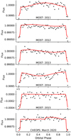 |
Fig. C.1 Comparison of the yearly MOST photometry from Sulis et al. (2019) with the CHEOPS observations in the bottom panel. The red curves for each MOST observation is a simple sinusoid and transit model, while the red curve for the CHEOPS observations represents the piecewise-Lambertian model. |
References
- Agol, E., Cowan, N. B., Knutson, H. A., et al. 2010, ApJ, 721, 1861 [NASA ADS] [CrossRef] [Google Scholar]
- Agol, E., Luger, R., & Foreman-Mackey, D. 2020, AJ, 159, 123 [Google Scholar]
- Angelo, I., & Hu, R. 2017, AJ, 154, 232 [NASA ADS] [CrossRef] [Google Scholar]
- Astropy Collaboration (Robitaille, T. P., et al.) 2013, A&A, 558, A33 [NASA ADS] [CrossRef] [EDP Sciences] [Google Scholar]
- Astropy Collaboration (Price-Whelan, A. M., et al.) 2018, AJ, 156, 123 [Google Scholar]
- Benz, W., Broeg, C., Fortier, A., et al. 2021, Exp. Astron., 51, 109 [Google Scholar]
- Berta, Z. K., Charbonneau, D., Désert, J.-M., et al. 2012, ApJ, 747, 35 [NASA ADS] [CrossRef] [Google Scholar]
- Betancourt, M. 2017, ArXiv e-prints [arXiv:1701.02434] [Google Scholar]
- Bourrier, V., Dumusque, X., Dorn, C., et al. 2018a, A&A, 619, A1 [NASA ADS] [CrossRef] [EDP Sciences] [Google Scholar]
- Bourrier, V., Ehrenreich, D., Lecavelier des Etangs, A., et al. 2018b, A&A, 615, A117 [NASA ADS] [CrossRef] [EDP Sciences] [Google Scholar]
- Dawson, R. I., & Fabrycky, D. C. 2010, ApJ, 722, 937 [NASA ADS] [CrossRef] [Google Scholar]
- Deibert, E. K., de Mooij, E. J. W., Jayawardhana, R., et al. 2021, AJ, 161, 209 [NASA ADS] [CrossRef] [Google Scholar]
- Deline, A., Queloz, D., Chazelas, B., et al. 2020, A&A, 635, A22 [NASA ADS] [CrossRef] [EDP Sciences] [Google Scholar]
- Deming, D. 2009, in Transiting Planets, eds. F. Pont, D. Sasselov, & M. J. Holman, 253, 197 [NASA ADS] [Google Scholar]
- Deming, D., Harrington, J., Seager, S., & Richardson, L. J. 2006, ApJ, 644, 560 [NASA ADS] [CrossRef] [MathSciNet] [Google Scholar]
- Demory, B. O., Gillon, M., Deming, D., et al. 2011, A&A, 533, A114 [NASA ADS] [CrossRef] [EDP Sciences] [Google Scholar]
- Demory, B.-O., Ehrenreich, D., Queloz, D., et al. 2015, MNRAS, 450, 2043 [NASA ADS] [CrossRef] [Google Scholar]
- Demory, B.-O., Gillon, M., de Wit, J., et al. 2016a, Nature, 532, 207 [NASA ADS] [CrossRef] [Google Scholar]
- Demory, B.-O., Gillon, M., Madhusudhan, N., & Queloz, D. 2016b, MNRAS, 455, 2018 [NASA ADS] [CrossRef] [Google Scholar]
- Désert, J.-M., Lecavelier des Etangs, A., Hébrard, G., et al. 2009, ApJ, 699, 478 [NASA ADS] [CrossRef] [Google Scholar]
- Dorn, C., Hinkel, N. R., & Venturini, J. 2017, A&A, 597, A38 [NASA ADS] [CrossRef] [EDP Sciences] [Google Scholar]
- Ehrenreich, D., Bourrier, V., Bonfils, X., et al. 2012, A&A, 547, A18 [NASA ADS] [CrossRef] [EDP Sciences] [Google Scholar]
- Esteves, L. J., de Mooij, E. J. W., Jayawardhana, R., Watson, C., & de Kok, R. 2017, AJ, 153, 268 [NASA ADS] [CrossRef] [Google Scholar]
- Fischer, D. A., Marcy, G. W., Butler, R. P., et al. 2008, ApJ, 675, 790 [Google Scholar]
- Folsom, C. P., Fionnagáin, D. Ó., Fossati, L., et al. 2020, A&A, 633, A48 [CrossRef] [EDP Sciences] [Google Scholar]
- Foreman-Mackey, D., Hogg, D. W., Lang, D., & Goodman, J. 2013, PASP, 125, 306 [Google Scholar]
- Foreman-Mackey, D., Luger, R., Czekala, I., et al. 2020, exoplanet-dev/exoplanet v0.3.2 [Google Scholar]
- Fulton, B. J., Petigura, E. A., Howard, A. W., et al. 2017, AJ, 154, 109 [Google Scholar]
- Futyan, D., Fortier, A., Beck, M., et al. 2020, A&A, 635, A23 [NASA ADS] [CrossRef] [EDP Sciences] [Google Scholar]
- Hammond, M., & Pierrehumbert, R. T. 2017, ApJ, 849, 152 [NASA ADS] [CrossRef] [Google Scholar]
- Harris, C. R., Millman, K. J., van der Walt, S. J., et al. 2020, Nature, 585, 357 [CrossRef] [PubMed] [Google Scholar]
- Heng, K., & Tsai, S.-M. 2016, ApJ, 829, 104 [NASA ADS] [CrossRef] [Google Scholar]
- Henry, G. W., Baliunas, S. L., Donahue, R. A., Fekel, F. C., & Soon, W. 2000, ApJ, 531, 415 [NASA ADS] [CrossRef] [Google Scholar]
- Hoyer, S., Guterman, P., Demangeon, O., et al. 2020, A&A, 635, A24 [NASA ADS] [CrossRef] [EDP Sciences] [Google Scholar]
- Hu, R., Demory, B.-O., Seager, S., Lewis, N., & Showman, A. P. 2015, ApJ, 802, 51 [Google Scholar]
- Hunter, J. D. 2007, Comput. Sci. Eng., 9, 90 [NASA ADS] [CrossRef] [Google Scholar]
- Jardine, M., & Collier Cameron A. 2008, A&A, 490, 843 [NASA ADS] [CrossRef] [EDP Sciences] [Google Scholar]
- Jindal, A., de Mooij, E. J. W., Jayawardhana, R., et al. 2020, AJ, 160, 101 [Google Scholar]
- Jones, E., Oliphant, T., Peterson, P., et al. 2001, SciPy: Open source scientific tools for Python [Google Scholar]
- Kipping, D. M. 2013, MNRAS, 435, 2152 [Google Scholar]
- Kipping, D., & Jansen, T. 2020, Res. Notes Am. Astron. Soc., 4, 170 [Google Scholar]
- Kite, E. S., Fegley, Bruce, J., Schaefer, L., & Gaidos, E. 2016, ApJ, 828, 80 [NASA ADS] [CrossRef] [Google Scholar]
- Knutson, H. A., Charbonneau, D., Allen, L. E., Burrows, A., & Megeath, S. T. 2008, ApJ, 673, 526 [Google Scholar]
- Kreidberg, L. 2015, PASP, 127, 1161 [NASA ADS] [CrossRef] [Google Scholar]
- Kumar, R., Carroll, C., Hartikainen, A., & Martin, O. 2019, J. Open Source Softw., 4, 1143 [Google Scholar]
- Lecavelier des Etangs, A., Vidal-Madjar, A., McConnell, J. C., & Hébrard, G. 2004, A&A, 418, L1 [NASA ADS] [CrossRef] [EDP Sciences] [Google Scholar]
- Lendl, M., Csizmadia, S., Deline, A., et al. 2020, A&A, 643, A94 [EDP Sciences] [Google Scholar]
- Luger, R., Agol, E., Foreman-Mackey, D., et al. 2019, AJ, 157, 64 [NASA ADS] [CrossRef] [Google Scholar]
- Madhusudhan, N., Lee, K. K. M., & Mousis, O. 2012, ApJ, 759, L40 [NASA ADS] [CrossRef] [Google Scholar]
- Mahapatra, G., Helling, C., & Miguel, Y. 2017, MNRAS, 472, 447 [NASA ADS] [CrossRef] [Google Scholar]
- McArthur, B. E., Endl, M., Cochran, W. D., et al. 2004, ApJ, 614, L81 [Google Scholar]
- McEwen, A. S., Keszthelyi, L., Geissler, P., et al. 1998, Icarus, 135, 181 [NASA ADS] [CrossRef] [Google Scholar]
- Miguel, Y. 2019, MNRAS, 482, 2893 [NASA ADS] [Google Scholar]
- Owen, J. E., & Wu, Y. 2017, ApJ, 847, 29 [Google Scholar]
- Pérez, F., & Granger, B. E. 2007, Comput. Sci. Eng., 9, 21 [Google Scholar]
- Ridden-Harper, A. R., Snellen, I. A. G., Keller, C. U., et al. 2016, A&A, 593, A129 [NASA ADS] [CrossRef] [EDP Sciences] [Google Scholar]
- Salvatier, J., Wiecki, T. V., & Fonnesbeck, C. 2016a, PeerJ Comput. Sci., 2, e55 [Google Scholar]
- Salvatier, J., Wieckiâ, T. V., & Fonnesbeck, C. 2016b, PyMC3: Python probabilistic programming framework [Google Scholar]
- Spencer, J. R., Sartoretti, P., Ballester, G. E., et al. 1997, Geophys. Res. Lett., 24, 2471 [NASA ADS] [CrossRef] [Google Scholar]
- Stevenson, K. B., & Eck, W. 2019, Pre-Flashing WFC3/IR Time-Series, Spatial Scan Observations, Space Telescope WFC Instrument Science Report [Google Scholar]
- Sulis, S., Dragomir, D., Lendl, M., et al. 2019, A&A, 631, A129 [NASA ADS] [CrossRef] [EDP Sciences] [Google Scholar]
- Tamburo, P., Mandell, A., Deming, D., & Garhart, E. 2018, AJ, 155, 221 [NASA ADS] [CrossRef] [Google Scholar]
- Theano Development Team 2016, ArXiv e-prints [arXiv:1605.02688]. [Google Scholar]
- Tsiaras, A., Rocchetto, M., Waldmann, I. P., et al. 2016, ApJ, 820, 99 [NASA ADS] [CrossRef] [Google Scholar]
- Van Eylen, V., Agentoft, C., Lundkvist, M. S., et al. 2018, MNRAS, 479, 4786 [Google Scholar]
- Vehtari, A., Gelman, A., & Gabry, J. 2017, Stat. Comput., 27, 1413 [Google Scholar]
- Venot, O., Hébrard, E., Agúndez, M., Decin, L., & Bounaceur, R. 2015, A&A, 577, A33 [NASA ADS] [CrossRef] [EDP Sciences] [Google Scholar]
- von Braun, K., Boyajian, T. S., ten Brummelaar, T. A., et al. 2011, ApJ, 740, 49 [NASA ADS] [CrossRef] [Google Scholar]
- Winn, J. N., Matthews, J. M., Dawson, R. I., et al. 2011, ApJ, 737, L18 [Google Scholar]
- Zarka, P. 2007, Planet. Space Sci., 55, 598 [NASA ADS] [CrossRef] [Google Scholar]
- Zhang, M., Knutson, H. A., Wang, L., et al. 2021, AJ, 161, 181 [NASA ADS] [CrossRef] [Google Scholar]
- Zhou, Y., Apai, D., Lew, B. W. P., & Schneider, G. 2017, AJ, 153, 243 [CrossRef] [Google Scholar]
- Zilinskas, M., Miguel, Y., Mollière, P., & Tsai, S.-M. 2020, MNRAS, 494, 1490 [CrossRef] [Google Scholar]
All Tables
CHEOPS observation logs, corresponding to the IOC observations in the first row and the phase curve observations in the second row.
Change in the Leave-One-Out Cross-Validation and Widely Applicable Information Criterion statistics between models compared with the best-fitting model, which is the piecewise-Lambertian model of Hu et al. (2015).
Comparison of the best-fit transit model parameters for the DRP and PSF photometric reductions.
All Figures
|
Fig. 1 Smear contamination correction. Top-left: an example CHEOPS exposure where the smear contamination from 53 Cnc, located outside the subarray image, is visible at the left of 55 Cnc (the star at the center of the field of view). Top-right: the same frame after the DRP v12 smear correction. Bottom: the estimated smear contamination flux within the DEFAULT aperture as a function of the observation roll angle which affects each orbit. |
| In the text | |
|
Fig. 2 Photometry from CHEOPS of 55 Cnc e and detrending vectors. (a) Raw fluxes returned by the Data Reduction Pipeline (DRP) aperture photometry observations over the 1.6 orbital phases of 55 Cnc e, centered on a transit. Red points are centroid outliers and are masked from analysis. The gaps in the observations occur primarily when Earth is occulting the target star. The horizontal dashed line at flux unity represents the median flux, about which we see variations in flux in the phase curve. (b) One component of the variations in the raw phase curve in panel a is a “ramp” feature which is anticorrelated with the telescope tube temperature, denoted the “ThermFront 2 Sensor” temperature. A full discussion of the link between the flux variations and telescope tube temperature is written in Sect. 3.3. The temperature of the telescope tube rises asymptotically from a minimum at the beginning of the observations to a near-constant value after ~ 0.5 days. There is an additional perturbation in the temperature once per orbit, thought to be caused by illumination of the telescope optical assembly by the Earth during occultation. (c) Changes in the DRP flux are associated with changes in the ThermFront 2 Sensor temperature after dividing out the transit with a slope of − 193 ± 10 ppm/degree Celsius. (d)Measured centroid of the target star on the detector in pixel units – outliers in red are masked from further analysis. (e) Trends in DRP flux with roll angle after correction for smearing (see Sect. 3.2) are ≲ 100 ppm, and are a result of correlations between the spacecraft roll angle and the contamination from nearby stars, and in the background light (see Sect. 3.2). Red points are the masked centroid outliers, which mostly occur immediately before and after the Earth occultation. |
| In the text | |
|
Fig. 3 Select posterior distributions for key parameters in the composite transit, eclipse and piecewise-Lambertian phase curve model. The parameters are the planet radius Rp, impact parameteter b, full amplitude of the phase variations, and the start and stop longitudes of the piecewise-Lambertian model ξ1, ξ2. The full posterior distribution correlation matrix is given in Appendix A. |
| In the text | |
|
Fig. 4 Detrended CHEOPS photometry of 55 Cnc e. Upper: the Data Reduction Pipeline (DRP) aperture photometry fluxes in black, and in red the best-fit linear combination of a transit model, a piecewise-Lambertian phase variation, and several detrending vectors. This fit is used to infer the best-fit transit parameters. The left column shows transit observations obtained during the in-orbit commissioning (IOC) phase, and the right column shows the phase curve observation. Middle: the residuals after the instrumental and systematic variations have been removed (black) and several draws from the posterior distributions for the transit and phase curve parameters (red). Lower: the residuals after removing allsystematics and astrophysical signals from the observations. |
| In the text | |
|
Fig. 5 Comparison of the different models tested (colored curves), compared to the best-fit residuals obtained for the sinusoidal model (gray, and binned once per CHEOPS orbit in black). |
| In the text | |
|
Fig. A.1 Posterior distributions and joint correlations between all free parameters in the joint fit to the In-Orbit Commissioning transit and phase curve observations sampled with the No U-Turn Sampler. The parameters include: the mid-transit time t0, limb-darkening parameters u0, u1, the ratio of planetary to stellar radius Rp∕R⋆, the impact parameter b, the eclipse depth δecl; two sets of detrending vector weights for the following vectors, one per visit: the ThermFront 2 temperature sensor reading, thecosine and sine of the roll angle, and a unit vector; the amplitude of the piecewise-Lambertian variations A; and the startand stop longitudes of the lower-reflectivity region ξ1 and ξ2. The last parameter, log σ is the natural logarithm of the flux uncertainty for each measurement. |
| In the text | |
|
Fig. B.1 Four principal components with the highest eigenvalues (from the PCA of the PSFs). |
| In the text | |
|
Fig. B.2 Relative coefficients of the U1 to U8 components from the PCA of the PSFs as a function of time. The roll angle dependence has been removed in this plot. |
| In the text | |
|
Fig. B.3 Relative coefficients of the U1 to U8 components from the PCA of the PSFs as a function of roll angle. The long-term time dependence from Fig. B.1 has been removed in this plot, to reduce the scatter and better see the roll angle trend. |
| In the text | |
|
Fig. B.4 CHEOPS PSF and its changes over the 55 Cnc e visit. The left panel shows the mean PSF, the central panel shows the standard deviation of the PSF per pixel over the duration of the visit, and the right panel shows the fractional change of the PSF per pixel. |
| In the text | |
|
Fig. B.5 Comparison of the CHEOPS Data Reduction Pipeline (DRP) aperture photometry (black) with the PIPE PSF photometry (gray). The PSF photometry is computed on the imagettes and therefore has a higher cadence than the DRP photometry.The In-Orbit Commissioning (IOC) transit observations are on the left, and the first 55 Cnc e phase curve observation is on the right. |
| In the text | |
|
Fig. C.1 Comparison of the yearly MOST photometry from Sulis et al. (2019) with the CHEOPS observations in the bottom panel. The red curves for each MOST observation is a simple sinusoid and transit model, while the red curve for the CHEOPS observations represents the piecewise-Lambertian model. |
| In the text | |
Current usage metrics show cumulative count of Article Views (full-text article views including HTML views, PDF and ePub downloads, according to the available data) and Abstracts Views on Vision4Press platform.
Data correspond to usage on the plateform after 2015. The current usage metrics is available 48-96 hours after online publication and is updated daily on week days.
Initial download of the metrics may take a while.