| Issue |
A&A
Volume 653, September 2021
|
|
|---|---|---|
| Article Number | A157 | |
| Number of page(s) | 21 | |
| Section | Interstellar and circumstellar matter | |
| DOI | https://doi.org/10.1051/0004-6361/202040053 | |
| Published online | 27 September 2021 | |
Strong dependence of the physical properties of cores on spatial resolution in observations and simulations
1
AIM, CEA, CNRS, Université Paris-Saclay, Université Paris Diderot,
Sorbonne Paris Cité,
91191
Gif-sur-Yvette,
France
e-mail: This email address is being protected from spambots. You need JavaScript enabled to view it.
2
LERMA (UMR CNRS 8112), École Normale Supérieure,
75231
Paris Cedex,
France
3
Scuola Normale Superiore di Pisa,
Piazza dei Cavalieri, 7,
56126
Pisa,
Italy
4
Université Grenoble Alpe, CNRS, IPAG,
38000
Grenoble,
France
Received:
3
December
2020
Accepted:
30
June
2021
Abstract
The angular resolution of a telescope is the primary observational parameter, along with the detector sensitivity in defining the quality of the observed images and of the subsequent scientific exploitation of the data. During the last decade in star formation research, many studies have targeted low- and high-mass star formation regions located at different distances, with different telescopes having specific angular resolution capabilities. However, no dedicated studies of the spatial resolution effects on the derived sizes and masses of the sources extracted from the observed images have been published. We present a systematic investigation of the angular resolution effects, with special attention being paid to the derived masses of sources as well as the shape of the resulting source mass functions (SMFs) and to their comparison with the initial stellar mass function. For our study, we chose two star-forming regions observed with Herschel, NGC 6334 and Aquila distant of 1750 and 460 pc respectively, and three (magneto)-hydrodynamical simulations, virtually positioned at the same distances as the observed regions. We built surface density maps with different angular resolutions by convolving the surface density images of the five regions to a set of four resolutions differing by a factor of two (9, 18, 36, and 72′′), which allowed us to cover spatial resolutions from 0.6 down to 0.02 pc. Then we detected and measured sources in each of the images at each resolution using getsf and we analysed the derived masses and sizes of the extracted sources. We find that the number of sources does not converge from 0.6 to ≳0.05 pc. It increases by about two when the angular resolution increases with a similar factor, which confirms that these large sources are cluster-forming clumps. Below 0.05 pc, the number of source still increases by about 1.3 when the angular resolution increases by two, suggesting that we are close to, but not yet at, convergence. In this regime of physical scales, we find that the measured sizes and masses of sources linearly depend on the angular resolution with no sign of convergence to a resolution-independent value, implying that these sources cannot be assimilated to isolated prestellar cores. The corresponding SMF peak also shifts with angular resolution, while the slope of the high-mass tail of the SMFs remains almost invariant. We propose that these angular resolution effects could be caused by the underestimated background of the unresolved sources observed against the sloping, hill-like backgrounds of the molecular clouds. If prestellar cores physically distinct from their background exist in cluster-forming molecular clouds, we conclude that their mass must be lower than reported so far in the literature. We discuss various implications for the studies of star formation: the problem of determining the mass reservoirs involved in the star-formation process; the inapplicability of the Gaussian beam deconvolution to infer source sizes; and the impossibility to determine the efficiency of the mass conversion from the cores to the stars. Our approach constitutes a simple convergence test to determine whether an observation is affected by angular resolution.
Key words: ISM: clouds / methods: numerical / methods: observational / stars: formation / infrared: ISM / techniques: image processing
© F. Louvet et al. 2021
 Open Access article, published by EDP Sciences, under the terms of the Creative Commons Attribution License (https://creativecommons.org/licenses/by/4.0), which permits unrestricted use, distribution, and reproduction in any medium, provided the original work is properly cited.
1 Introduction
One of the challenges of modern astrophysics is to understand what controls the mass distribution of stars at their birth, the so-called initial mass function (IMF). Most of the observational studies since the work of Salpeter (1955) have found the shape of the IMF to be universal (e.g. Kroupa 2002; Lada & Lada 2003; Bastian et al. 2010), except possibly in young massive clusters (e.g. Lu et al. 2013; Schneider et al. 2018). Understanding its origin is crucial for both star formation and galactic evolution. The IMF exhibits a peak at mass M ≈ 0.3 M⊙ and a power-law high-mass end dN∕d log(M) ∝ M−1.35. Similarities between the slope of the IMF and the slope of the core mass function (CMF), derived from observations of molecular clouds, led to the suggestion that the IMF results from the fragmentation of molecular clouds (e.g. Motte et al. 1998; Testi & Sargent 1998; Alves et al. 2007; Könyves et al. 2015, 2020). Such similarities have also been reported in numerical studies (e.g. Klessen 2001; Tilley & Pudritz 2004; Ntormousi & Hennebelle 2019).
With the possibility of a relationship between the IMF and the CMF, studies on the origin of the IMF proceeded in two directions: to understand (1) the origin of the CMF and its link with the fragmentation processes of molecular clouds (e.g. Padoan et al. 2007; Schmidt et al. 2010) and (2) the connection between the prestellar cores and stars (e.g. Smith et al. 2009; Lomax et al. 2014; Pelkonen et al. 2021), with a commonly used broad assumption of a one-to-one correspondence between the two types of objects. The assumption means that the gravitational collapse of a prestellar core forms a single star or a close binary, with a certain mass transfer efficiency from the core to the stars (e.g. Padoan et al. 1997; Hennebelle & Chabrier 2008; Hopkins 2012). In this picture of star formation, the cores must remain not fragmented during the collapse. It is believed that prestellar cores are the result of gravo-thermal fragmentation in molecular clouds, resulting in an average core mass of ~ 2 M⊙ and size of ~0.2 pc that correspond to the Jeans mass and length for gas with a temperature and mean density of T ≃ 10 K and  104 cm−3, typical of dense regions in molecular clouds.
Modern high-resolution and sensitive imaging in the far-infrared and sub-millimetre wavelengths led to a standard approach to their analysis. In that approach, the single or multi-wavelength images of star-forming regions are analysed using source extraction methods. The extraction tools detect, measure, and catalogue all sources of emissions inthe images, that is, all strong intensity peaks that stand out against the local background and noise fluctuations.
Despite the importance of the angular resolutions for observational studies of star formation, no detailed systematic study has been done to clarify their effects on the derived properties of the physical objects. We investigate how the sizes and masses of the same sources behave when analysed at different spatial resolutions. We extracted and examined sources at different angular resolutions in the NGC 6334 high-mass star-forming region and in the Aquila low-mass star-forming region. Because they are physically different and present very different resolutions, these two regions are highly complementary for our analysis. In particular the sources in NGC 6334 are likely to be small clumps while the sources of Aquila have been described in the literature as candidatepre- and protostellar dense cores. These two sets of observations complement the analysis with a similar approach using numerical simulations that allowed us to reach higher angular resolutions and to assess the impact of the projection effects. In Sect. 2, we present the different observational and numerical data sets that we used. In Sect. 3, we show that angular resolution affects the properties of extracted sources, even at scales lower than 0.05 pc where we expect to retrieve candidate prestellar cores. In Sect. 4, we discuss the similarities and differences between observations and simulations and put our study in perspective with recent investigations on the link between the CMF and the IMF. In Sect. 5, we summarise our conclusions.
2 Observations and numerical simulations
This paper aims to investigate the effect of angular resolution on the properties of sources and resulting source mass function (SMF), from large scale (0.6 pc) where we expect to observe cluster-forming clumps down to small-scales (≲0.05 pc) where we expect to see individual pre-stellar cores. To that end, we use Herschel observations and numerical simulations of both low- and high-mass star-forming regions to understand the effects of angular resolution on the derivation of the physical parameters of the gravitationally bound sources, in the framework of the standard observational approach of source extractions.
2.1 A high-mass star-forming region: NGC 6334
NGC 6334 is a complex of giant molecular clouds in the Sagittarius-Carina arm of the Milky Way, with an estimated mass M ≃ 7 × 10⁵ M⊙ (e.g. Russeil et al. 2012), located at a distance D ≃ 1.75 kpc from the Sun (Matthews et al. 2008). This very active high-mass star-forming region hosts more than 2000 young stellar objects (YSOs) identified with Spitzer (Willis et al. 2013), numerous H II regions, maser sources, and molecular outflows (see Loughran et al. 1986; Carral et al. 2002; Persi & Tapia 2008; Louvet et al. 2019). In this paper, we use a column density image of NGC 6334, derived from the Herschel images at 160, 250, 350, and 500 μm with an effective angular resolution of 18′′ from the HOBYS key programme (Motte et al. 2010)1. We extracted and analysed sources detected in the surface density map at the initial 18′′ resolution and after degrading the image to the 36 and 72′′ resolutions (Fig. 1, Sect. 3.2).
2.2 A low-mass star-forming region: Aquila
Aquila is a complex of molecular clouds at the end of the Aquila rift, located at a distance of 435– 490 pc (see Ortiz-León et al. 2017; Zucker et al. 2020, respectively). In this study we adopt a distance of 460 pc. Using the 2MASS extinction maps, Bontemps et al. (2010) derived its total mass M ≃ 9 × 10⁴ M⊙2 and, using the Herschel 70 and 160 μm images, they identified about 200 YSOs in Aquila. In this work, we use the high-resolution column density map presented in Könyves et al. (2015). This map has a native angular resolution of 18′′. It was built from the Herschel images at 160, 250, 350, and 500 μm taken during the Herschel Gould Belt Survey (HGBS, see André et al. 2010). We extracted and analysed sources in the surface density image at the initial 18′′ resolution and after degrading the image tothe 36 and 72′′ resolutions (Fig. 2, Sect. 3.2).
2.3 Simulations of star-forming regions
To overcome the limited angular resolution provided by currently available telescopes, we employed several numerical simulations of a 3D turbulent cloud designed to represent an Orion-sized molecular cloud (Ntormousi & Hennebelle 2019, hereafter NH19). They were produced with the RAMSES code (Teyssier 2002; Fromang et al. 2006) that solves the magneto-hydrodynamical (MHD) equations on a Cartesian grid with adaptive mesh refinement (AMR).
The initial conditions of the simulations resembled a molecular cloud, that was approximated by an ellipsoid with a full extent of 33 pc × 13.2 pc × 13.2 pc and a mass of 105 M⊙, with a volume density profile defined by
 (1)
(1)
where  is the radial coordinate and (z0, r0) is the point at which the density profile flattens to ρ0 = 1500 cm−3, the initial peak density in the cloud. The simulations were computed on an adaptive mesh, such that they always resolve the Jeans length with at least ten cells. The coarsest 5123 grid occupied a volume of 663 pc3.
We performed two hydrodynamical simulations (HD, HDh) and one magneto-hydrodynamical simulation (MHD) with a magnetic field that was initially oriented along the x-axis. The HD and MHD runs had 7 additional levels of mesh refinement and the high-resolution HDh run used 8 additional refinement levels, corresponding to the maximum resolutions of ~ 400 and 200 au, respectively. The models included sink particles that approximate the evolution of unresolved small scales by an immediate collapse onto a point mass (Bleuler & Teyssier 2014). These sink particles are disconnected from the hydrodynamical evolution and interactwith the remaining gas through gravity and accretion only. New sink particles form when the volume density exceeds 108 cm−3 (HD, MHD) or 109 cm−3 (HDh) and when the gas inside a small volume around the density peak undergoes gravitational collapse. With these formation criteria, the sink particles may be considered as individual protostars. However, the stellar feedback is not included and the models used an isothermal equation of state. The parameters of the simulations are listed in Table 1 and a more detailed description of the models is presented in NH19.
For a meaningful comparison of the numerical simulations with real observations, it is necessary to convert their numerical output into a form that resembles the observations. We isolated the inner parts of the numerical boxes, limited by ± 0.5xmax, ± 0.5ymax, and ± 0.5zmax, containing most of the dense gas. These boxes were projected onto the grids of 4096 × 4096 pixels for the HD and MHD simulations and 8192 × 8192 pixels for HDh along the x, y, and z axes, allowing us to investigate the projection effects (Sect. 3.4). The pixel units of the resulting surface density maps were converted from pc to arcsec, using the distances of 1750 pc for the H and MHD models and 460 pc for HDh, corresponding to NGC 6334 and Aquila, respectively. A uniform Gaussian noise was added to the resulting surface densities, at the levels corresponding to the first quartile of the image pixel distributions (~ 1021 cm−2). The maps were smoothed to the 9, 18, 36, and 72′′ resolutions for the HD, MHD, and HDh simulations, which cover the angular resolutions of the observed regions. In total, we obtained 36 synthetic surface density images for the HD, MHD, and HDh simulations. The surface density maps projected along the x axis for HD and HDh are shown in Figs. 3 and 4, whereas the maps for the other projections and for MHD are presented in Appendix A.
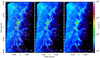 |
Fig. 1 Column densities of the high-mass star-forming region NGC 6334 (D ≃ 1750 pc). The imagesare overlaid with the half-maximum ellipses of the extracted bound sources (Sect. 3.1), with the angular resolutions indicated in each panel. The red rectangle in the left panel indicates the central region of NGC 6334 discussed in Sect. 4.1. |
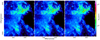 |
Fig. 2 Column densities of the low-mass star-forming region Aquila (D ≃ 460 pc). The images are overlaid with the half-maximum ellipses of the extracted bound sources (Sect. 3.1), with the angular resolutions indicated in each panel. |
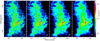 |
Fig. 3 Column densities obtained by projecting the HD simulation along the x axis, overlaid with the half-maximum ellipses of the extracted bound sources (Sect. 3.1). The angular resolutions, indicated in the panels, correspond to the linear scales of 0.07, 0.15, 0.3, and 0.6 pc. |
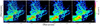 |
Fig. 4 Surface densities obtained by projecting the HDh simulation along the x axis, overlaid with the half-maximum ellipses of the extracted bound sources (Sect. 3.1). The angular resolutions, indicated in the panels, correspond to linear scales of 0.02, 0.04, 0.08, and 0.16 pc. |
Parameters of the numerical simulations.
3 Extraction and analysis of sources
The column density images of the observed and simulated star-forming regions were given as an input to a source extraction algorithm that produced catalogues of sources, from which we selected self-gravitating sources. In the following, we describe the angular resolution effects on the measured sizes and masses of the selected sources and the resulting source mass function (SMF). We present the results obtained for the observed fields, NGC 6334 and Aquila, and we analyse the results for the HD, MHD, and HDh simulations to follow the resolution effects beyond the angular resolutions accessible in present-day observations.
3.1 Identification and selection of sources
To extract sources in the observed and simulated images, we used the new multi-scale source and filament extraction method getsf (Men’shchikov 2021). The method is the successor of getsources, getfilaments, and getimages (Men’shchikov et al. 2012; Men’shchikov 2013, 2017) that have been widely used, primarily in the studies of low- and high-mass star formation with Herschel. This method decomposes spatially the image(s) to effectively isolate structures of different widths and shapes. It separates the structural components of sources, filaments, and their backgrounds. Having separated the three components, getsf flattens the sources and filaments images to produce the flat detection images with uniform fluctuations over the images. Then it applies thresholding to remove insignificant fluctuations and uses only significant peaks to detect sources. Finally, it measures detected sources in the original images after subtracting their background and after deblending the sources. The getsf method only takes one input parameter: the maximum size of sources of interest, that the user determines from the images. The value of this parameter affects marginally the extraction results. The method is publicly available on its website3 and fully described in Men’shchikov (2021).
The column density integrated over the source area at the adopted distance D gives the source mass MS. We use the half-maximum sizes A and B (FWHM) to obtain the equivalent spherical radius RS of the source with the volume πAB2∕6. To determine whether a source may be considered as gravitationally bound (self-gravitating) we followed Könyves et al. (2015) and computed the ratio  between the source mass and the critical Bonnor-Ebert mass:
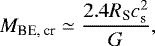 (2)
(2)
where RS is the source radius, cs the sound speed at T = 20 K, and G the gravitational constant. The sources with αBE < 2 were considered as self-gravitating, hereafter called bound sources for brevity. In the analysis below we consider only the bound sources. In all column density maps (Figs. 1–4 and A.1–A.3), bound sources are shown by their ellipses, whose major and minor axes are equal to the source sizes A and B that are estimated by getsf at half-maximum intensity after subtraction of the sources background. The extraction results for all regions (NGC 6334, Aquila, simulations HD, MHD, and HDh) and angular resolutions are summarised in Table 2.
Source extractions in the observed and simulated regions at different angular resolutions.
3.2 Angular resolution effects in observations
Figures 1 and 2 show the surface density maps of NGC 6334 and Aquila at three angular resolutions, differing by a factor of two. The maps are overlaid with the half-maximum ellipses of the bound sources. In both cases, the coarser the angular resolution, the fewer bound sources are found. Figure 5 presents the ratio of bound sources from one scale to the next: NB(2O)∕NB(O). The fragmentation cascade decreases with increasing spatial resolution for both NGC 6334 and Aquila. The effect is the strongest in NGC 6334. We argue it is because the physical scales we probe in NGC 6334 are larger than those we probe in Aquila.
Figure 6 demonstrates that degrading angular resolution affects the measured sizes of the sources. As a result of the angular resolution being lower by a factor of two, the average size of sources becomes twice larger. The mean size of the sources is of approximately 1.5 times the beam size for the three angular resolutions investigated. The size distribution is well represented by a lognormal distribution with a standard deviation of ~ 15% (Fig. 6), attributable to statistical fluctuations.
The changes in angular resolution also affect the masses of sources. If the surface density were uniform, and without blending of sources, twice larger sizes would imply sources four times more massive. In Aquila, where decreasing the angular resolution by a factor of two only blends together about 30% of the sources, this degradation of the resolution leads to sources that are, on average, two times more massive, which suggests that sources are centrally peaked. In NGC 6334, the downgrading of the resolution by a factor of four produces one extremely massive source (≳ 5 × 10⁴ M⊙) that bias the mean mass estimate. If we ignore this object, then the resolution lowered by successive factors of two corresponds to sources being consecutively three and five times more massive (see Fig. 5). This is a joint effect of the inclusion of the background emission into the source emission (see below) and of the blending of sources. The resolution dependence of the measured source mass is reflected in the derived source mass function: Fig. 6 shows a clear shift of the SMF towards higher masses for lower resolutions in both star-forming regions, NGC 6334 and Aquila.
The cumulative form of the SMFs (Fig. 6) exhibits the same shift towards higher mass for lower angular resolutions. Interestingly, the slope of the high-mass tail of the SMF is almost unaffected by the resolution changes: the best fit of the high-mass tail of the cumulative SMFs of NGC 6334 is very similar for the three angular resolutions, with α ≃ −1.06 ± 0.05. The slope is flatter than the α = −1.35 for the canonical IMF, in line with the recent estimates for high-mass star-forming regions, that give flatter slopes than those for the low-mass star-forming regions (see, e.g. Motte et al. 2018; Liu et al. 2018; Cheng et al. 2018; Sanhueza et al. 2019; Massi et al. 2019; Kong 2019; Servajean et al. 2019; Moser et al. 2020). The fits to the cumulative CMFs for Aquila are also almost invariant with respect to the angular resolution, with an index α ≃ −1.32 ± 0.07 indistinguishable from the slope of the canonical IMF, as previously reported by Könyves et al. (2015).
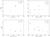 |
Fig. 5 Each data point represents the ratio, R = F(2O)∕F(O), at the spatial resolutions O and 2O of either the number (top, F = NB) or mean mass (bottom, |

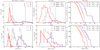 |
Fig. 6 Effects of different angular resolutions on the derived sizes and masses of bound sources in the star-forming regions NGC 6334 (top) and Aquila (bottom). We show the source size function (left), the source mass function (middle), and the cumulative mass function (right). The dashed curves in the left panels are the lognormal fits to the source size distributions and the vertical lines indicate the median values for each distribution. The dashed lines in the right panels are the fits to the cumulative SMFs within the range 5− 50%. For NGC 6334 (resp. Aquila), these intervals correspond to 14–107 M⊙ (resp. 1–4) at 18′′, 54–418 M⊙ (resp. 2–11) at 36′′, and 323-1870 M⊙ (resp. 4–20) at 72′′. |
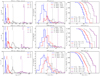 |
Fig. 7 Effects of different angular resolutions on the sizes and masses of bound sources in the simulated star-forming regions HD (top), MHD (middle row), and HDh (bottom). We show the source size function (left), the source mass function (middle), and the cumulative mass function (right), obtained for the y projection of the respective column density maps. The other projections on the x and z directions are displayed in Figs. A.7 and A.8. The fits of the cumulative SMFs were done only for extractions with more than 40 bound sources. We fitted the cumulative SMFs in the mass range corresponding to 5–50% of the source samples; it corresponds to, from top to bottom: 40–128, 39–125, 5–19 M⊙ for the blue curves, 94–304, 76–329, 11–49 M⊙ for the red curves, 28–120 M⊙ for the grey curve, and 87–537 M⊙ for the purple curve. |
3.3 Angular resolution effects in simulations
Figure 7 displays the sizes, masses, and cumulative source mass functions, obtained from the source extractions for the y projection of the HD, MHD, and HDh simulations; the x and z projections are presented in Appendix A. Similarly to the observed maps, the number of sources decreases for all simulations when the resolution is degraded by a factor of two. This decrease is all the more pronounced the larger the spatial scales we probe (see Table 2 and Fig. 5).
The simulations show the same behaviour as the observed regions with respect to the measured sizes of the extracted sources. For all angular resolutions, the mean size of sources systematically peaks at approximately 1.5 times the beam size, with a spread that follows a lognormal distribution with a standard deviation of 5% (Fig. 7). Therefore, the degradation of the angular resolution by a factor of two leads to sources whose average half-maximum sizes are twice larger. This effect leads to an increase in source masses.
As in the observed regions, downgrading the angular resolution by a factor of two makes the average mass of the extracted sources larger, by a factor of two at spatial scales smaller than 0.03 pc and up to a factor five a scales greater than 0.3 pc (see Fig. 5). The smaller statistics at lower resolutions and the increased masses of the sources strongly affect the peak of the SMF, shifting the latter towards higher masses (Fig. 7). The high-mass slope of the SMF is almost unaffected by the resolution changes (variations within ~ 10%) and no clear trends as long as the numbers of sources NS ≳ 40.
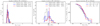 |
Fig. 8 Derived size and mass functions of the bound cores extracted by getsf from the column densities at 18′′ resolution, obtained from the HD simulation along the x, y, and z axes. The vertical dashed lines indicate the median size or mass; the cumulative form of the mass functions were fit by power laws in the range of 5− 50%. |
3.4 Viewing angle effects in the simulations
To understand whether the viewing angle at which a 3D molecular cloud is observed affects the numbers, masses, and sizes of the extracted sources, we compared the source extractions for the x, y, and z projections for all simulated regions (HD, MHD, and HDh) and angular resolutions (9, 18, 36, and 72′′). For an illustration, we selected the HD simulation at the resolution of 18′′ in Fig. 8, well representing the results; the other simulations and projections are presented in Appendix A.
The half-maximum sizes of the extracted sources show little variations (< 5%) from one projection to another (Fig. 8), as evidenced by the source size functions (SSFs) in the reference case (HD simulation at 18′′ resolution). The number of sources and their mean masses vary within 20− 25% between projections. For the reference case, we extracted an average number of 90 ± 24 sources with a median mass of 94 ± 25 M⊙. Such variations induce small displacements between the SMFs of the different projections (Fig. 8). A power-law fit of the high-mass tail of the cumulative form of the SMF (Fig. 8) yields the mean slope α ≃ −1.58 that varies by ~20% between the projections.
The variations in the numbers of extracted sources and mean masses increase as the resolution degrades. This is a pure statistical effect caused by the disappearance of unresolved sources, diluted by insufficient angular resolutions (Sects. 3.2 and 3.3, and Table 2). The differences in the properties of sources from one projection to another are less prominent when considering only the extractions with more than 40 sources. In such extractions, the number of identified bound sources varies by ~ 15%, their mean mass by ~20%, and the SMF slope by ~10%. It is reasonable to assume that the projection effects are moderate, but not negligible, for statistically significant samples of sources.
4 Discussion
Below, we discuss the results of our study, compare them with previous works, and analyse the reasons behind the very strong dependence of the properties of extracted sources on angular resolution.
4.1 Comparison between observed and simulated regions
Apart from one apparent discrepancy (see below) the effect of angular resolution on the derived properties of bound sources is the same in observations and numerical experiments. Among the resolutions common to the observations and simulations (18, 36, and 72′′), the number of bound sources and their mean size and mass strongly depend on the resolution at which the sources are extracted. As a consequence, the peak of the source mass function is also resolution-dependent, whereas the slope of the SMF is only marginally affected. Interestingly, in the numerical experiments at the highest angular resolution (9′′), exceeding the resolutions probed in the observed regions, we witness the same displacement of the SMFs. The number of extracted sources and their size and mass distributions respond to the increase of angular resolution in exactly the same way as at lower angular resolutions (Sect. 3.3).
Comparing our results for NGC 6334 with those for HD and MHD at the same angular resolutions, the main difference between the simulated and observed regions is in the source mass. For instance, the median mass of sources in NGC 6334 at 18′′ is 15 M⊙, whereas the median mass in HD and MHD are ~95 and ~ 110 M⊙, respectively (Table 2). This difference is mainly caused by the dissimilar sizes of the regions: the observed region is roughly 6 times larger and includes a large fraction of low- and intermediate column densities. Restricting the analysis for NGC 6334 to its densest region (the red rectangle in Fig. 1) with the same area as in the numerical experiments, we derive a median source mass of ~ 75 M⊙, compatible with those obtained in the simulations (Fig. 9). The high-mass slope of the SMF α ≃ −1 is estimated in NGC 6334, whereas α ≃ −1.35 is found in the simulated regions. The difference is even larger, when we restrict the analysis to the central dense area of NGC 6334, thereby removing a large fraction of the low- and intermediate-mass sources from the sample (Fig. 9). Statistically, there is an excess of massive sources in NGC 6334 with respect to those found in theHD and MHD simulated regions. This discrepancy might expose missing physics in the simulations, because their initial conditions match the properties of NGC 6334 (Sects. 2.1 and 2.3).
This difference is unimportant for this study, that does not aim at reproducing all details of the observed regions with numerical simulations. We systematically investigated how different angular resolutions affect the derived parameters of extracted sources in the observed and simulated regions across similar physical scales. In that aspect, our results demonstrate full consistency between observations and simulations.
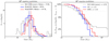 |
Fig. 9 Comparisons of the mass functions at 18′′ of the bound sources extracted by getsf in the star-forming regions NGC 6334 with those extracted in the HD (blue) and MHD (red) simulations. In case of NGC 6334, only the sources from the central region (red box in Fig. 1) were used. The numbers of sources were normalised to the peak of the mass function for NGC 6334 and the fits of the cumulative mass function were done within the range 10−50%. In all modelhistograms, the numbers of sources were averaged between the x, y, and z projections. |
4.2 Comparisons with previous source extractions
Tigé et al. (2017) analysed NGC 6334 during the HOBYS project (Motte et al. 2010) with an effective angular resolution of 18′′. Their strategy differs from ours: they detected sources with getsources (Men’shchikov et al. 2012) using the Herschel images from 160−500μm plus a column density map to detect sources, and measured the source fluxes from all available data: Herschel bands from 70− 500μm, JCMT, APEX, SEST, Spitzer, WISE, and MSX. Then, they built SED spectrum for each of the 4733 sources getsources detected, and applied different criteria to refine the source selection. Therefore the source catalogue comparisons given below must be considered as indicative. They classified the 490 most massive sources, with a median mass of 32 M⊙, which is consistent with the 940 sources of our sample with a median mass of 15 M⊙ taking into account the differences in the two approaches. Indeed, considering only the 490 most massive sources of our sample, the median mass becomes about 30 M⊙.
Könyves et al. (2015) investigated Aquila based on Herschel observations. They applied getsources to the Herschel images at 160−500μm and to a column density image. Several criteria were used to classify the extracted sources between YSOs, starless cores, and protostellar cores. In total, they reported 650 starless cores and 60 protostellar cores in the Aquila molecular cloud. To associate the sources with the self-gravitating starless cores, they used the ratio αBE between the source mass and the critical Bonnor-Ebert mass (see Eq. (2)). With their condition αBE < 2 they have found 290 prestellar cores, in good agreement with the 255 sources we found. Besides, they have reported a slope of the high-mass tail of the SMF of α ≃ −1.33, very similar to the mean slope ⟨α⟩ = −1.32 that we found between the 72 and 18′′ resolutions (Sect. 2.2). We stress, nevertheless, that their detection and measurement strategies differed from ours. They detected the sources using all the individual bands of Herschel besides the column density image in the one hand and computed the mass of the sources from SED fitting in the other. Hence the source catalogue comparisons must be considered as indicative only.
4.3 Interpretation of the angular resolution effects
The results of our systematic investigation of the properties of sources extracted at different angular resolutions may seem surprising, if we do not make a clear distinction between sources of emission, observed with a certain angular resolution, and decoupled cores in space that may be contributing to the observed peaks. If we follow one of the standard observational practices and equate a bound source whose size is smaller than ~0.05 pc with the pre- or proto-stellar core, its mass and size should no longer vary when increasing the telescope resolution. However, a careful analysis of the dependencies found in both observed and simulated regions suggests a coherent and natural interpretation4.
Comparing the images from the highest to the lowest resolution, we see that the number of sources drops faster and faster when the resolution is successively degraded by factors of two (cf. Table 2). The sources dilute within the larger beams and their emission merges with the background emission (Figs. 1–4, A.1–A.3). Therefore, the sources extracted at 72′′ resolution in Aquila or in the model HDh contain the emission of their background, and the contribution from the blended clusters of sources identified in the higher-resolution images.
Comparing the images from the lowest to the highest resolution, we see that the very large sources disappear or split into several sources and that many new sources appear. The appearance of new sources and the splitting of existing sources span from 72 to 18′′ in both observations and simulations (Figs. 1–4, A.1–A.3). In the numerical simulations, where we also have 9′′ synthetic observations, this behaviour continues from the 18 to the 9′′ angular resolution.
Large numbers of filaments in the observed regions and produced by the simulations also experience similar transformations. The filaments are the widest at the 72′′ resolution and they become increasingly sub-structured into a finer web of narrower filaments at higher angular resolutions. The increasing structural complexity of the filamentary background continues down to the smallest spatial scales we studied: 0.02pc in the numerical simulations, 0.04 pc in Aquila, and 0.15 pc in NGC 6334 (see Fig. 5).
Our results show that the majority of extracted sources appear more extended than the observational beam (by a factor of 1.5). If coreswith definite boundaries do exist they must actually be unresolved in all images and for all resolutions, because the average size of the extracted sources closely follows the angular resolution (Table 2). If the sources were resolved, their sizes would remain invariant with respect to the increasing resolution. Furthermore, the measured masses of the extracted sources also follow the angular resolution, changing by a factor of 2 even when the number of sources seems to approach convergence (Table 2). This means that the integrated emission of a source must contain a major contribution of either the dense and variable background, or of an unresolved cluster of smaller objects, or both.
The true background under extracted sources is fundamentally unknown: any information about the physical background of an unresolved source is diluted within the observational beam. This leads to major uncertainties in the measurement of source parameters5, especially their masses (or integrated fluxes). Self-gravitating prestellar cores form in the dense parts of the molecular clouds that fluctuate on all spatial scales, including the scale of the cores and below. In theory, they are expected to appear in the local density enhancements of the clouds or in dense filaments, hence, the environment of prestellar cores should resemble a hill. Therefore, source extraction tools would underestimate their background, because they interpolate it based on the values just outside the source (see Sect. 4.4). This means that the background-subtracted sources must contain some background contribution that could become quite large for faint unresolved sources.
We did not find any clear sign of convergence in the mass values across the entire range of resolutions that we investigated (see Fig. 5). Therefore, the currently available angular resolutions are probably insufficient to determine the correct mass of isolated prestellar cores, well decoupled from the background. If such decoupled cores exist in cluster-forming molecular clouds, they must be lighter than what we measured for unresolved sources.
We created a simple model (Fig. 10) to verify and illustrate our interpretation. An unresolved round Gaussian source with a half-maximum A = 3′′, peak value  cm−2, and mass MS = 0.13 M⊙ was added to a long filament with a crest density of 1023 cm−2 and a relatively shallow, slowly varying radial profile. The exact profile, peak density, and width of the source are unimportant, provided that it raises above the background by a factor of several and remains unresolved at the 9′′ resolution. The filamentary shape of the background is unimportant: it may also be modelled as a round peak with a similar radial profile. The model image was convolved with Gaussian beams to the angular resolutions of 4.5, 9, 18, 36, 72, and 144′′. For each image with different angular resolution, the source was background-subtracted with the algorithm used by getsf and its half-maximum size and mass were measured. The profiles of the model, of the background, and of the true and background-subtracted source are displayed in Fig. 10.
The sloping background of the model source leads to systematic, resolution-dependent inaccuracies of the derived background, which becomes progressively more underestimated towards lower resolutions (by the factors 1.15, 1.28, 1.52, 1.84, 2.35, and 3.37, respectively). The interpolated surface cuts too deep into the true background and, in effect, transfers substantial mass to the unresolved source and leads to a widening of the extracted sources. In the sequence of decreasing angular resolutions, the source becomes more extended than the original model source convolved to the same resolution, by the factors 1.005, 1.077, 1.13, 1.31, 1.45, and 1.50, respectively. At the lower resolutions (36, 72, and 144′′), when the unresolved source becomes more strongly diluted within the beam, the factors become very similar to the factor of approximately 1.5 that we found for the observed and simulated regions. In the same sequence of decreasing resolutions, the extracted source mass becomes 1.007, 1.089, 1.69, 4.14, 14.4, and 59.3 the mass of the source model. From one resolution to the next, it corresponds to a mass increase by the factors 1.08, 1.55, 2.45, 3.48, and 4.12. The results of our simple model resemble those obtained in this work, telling us that the measured masses of unresolved sources, located on bright fluctuating backgrounds, may be veryinaccurate.
This agreement of the toy-model with the results of this work confirms that our interpretation captures the essence of the resolution effects. However, this simple model cannot be considered as fully realistic in view of the presence of a large variety of complex structures and backgrounds in the observed and simulated images. For instance, it does not include the additional effects of unresolved background fluctuations, or blending of clusters into single sources at lower resolutions.
 |
Fig. 10 Simple model explaining the angular resolution effects on the derived masses and sizes of the sources located on top of filaments or other background fluctuations. The model image, consisting of an unresolved source on top of a filament, was convolved to different resolutions using Gaussian beams (FWHM), indicated in the panels. Shown are the radial profiles of the model across the filament (left), the getsf -interpolated background of the source (middle), and the background-subtracted source (right). The true radial profile of the model source and filament is shown by the thick dotted line. The background was interpolated within a radius of 1.25 times the resolution, which fully encircles the true source convolved to the resolution. Derived mass of the background-subtracted source increases by the factors 1.08, 1.55, 2.45, 3.48, and 4.12, when degrading the resolution by a factor of two. At each resolution, the measured half-maximum size
|

4.4 Comparison to other extraction algorithms
We solely used getsf (see Sect. 3.1) to conduct the source extractions but various algorithms have been used in star-formation studies: gaussclumps (Stutzki & Guesten 1990), clumpfind (Williams et al. 1994), dendrograms (Rosolowsky et al. 2008), cutex (Molinari et al. 2011), csar (Kirk et al. 2013), and fellwalker (Berry 2015). They employ different approaches: clumpfind and dendrograms analyse isointensity contours in the image; cutex analyses second derivative images to identify peaks; csar and fellwalker associate pixels one by one to local maxima. Two of these algorithms – clumpfind and fellwalker – do not subtract the background from sources. They are therefore irrelevant regarding angular resolution effects and background inclusion into the flux of sources.
The individual background of sources is unknown and differs for sources lying in different areas of a molecular cloud. Therefore, the background can only be estimated from the pixels outside the source. Gaussclumps, csar and dendrograms6 subtract the value at the border of the source. Cutex fits a Gaussian plus an inclined plane to the peak of each source, thereby removing this planar background. Getsf interpolates the source background along 4 diagonals linking the pixels just outside the sources, averages the interpolated values and estimates a non-planar background. Background of sources are highly uncertain, progressively more so for fainter sources. The problem is especially serious for embedded sources that are part of a cloud or part of a filament embedded in a cloud.
The different methods of background subtraction are accompanied by other differences in the extraction methods, the most important of them being deblending of overlapping sources. Only cutex and getsf deblend sources, whereas the other methods just partition the image between sources, not allowing them to overlap. These differences would engender dissimilarities in the results, such as the numbers of extracted sources and spurious sources, extraction completeness, inaccuracies in flux and mass measurements.
Regarding our problem on how angular resolution affects the sources features, we can separate the algorithms in two families: those fitting the emission peaks (cutex, gaussclumps, getsf), and those progressively associating the emission to local maxima (csar, dendrograms). For the first family, the smoothing of the map will (i) artificially increase the sources flux due to the inclusion of background emission (see Sect. 4.3) and (ii) reduce the number of detected sources as they dilute into the background. In the second family, sources extend until they reach a user-defined intensity threshold, or until they meet another source. When the angular resolution degrades, the faint sources will blend into the background. As a consequence, the sources that remain detectable will extend further away. These sources will appear even bigger, and more massive, than with fitting methods. The issue we report, that angular resolution affects source features, is generic, present at the data level, and independent of the source extraction algorithms.
4.5 Implications for the studies of star formation
The results, presented in this paper, imply that the masses of cores, derived for various star-forming regions in the recent years are likely overestimated. There are various consequences of this finding for the standard approach used in the observational studies of star formation. Below, we touch upon some of the important issues.
Our study shows that extracted sources must be unresolved even in the nearby star-forming regions, although the measured sizes seem to indicate the contrary. As shown by our results and explained in Sect. 4.3, the sources size at 1.5 times the beam is caused by an insufficient angular resolution in the presence of a complex sloping background. This means that the standard practice of determining the sizes of the physical cores by Gaussian beam deconvolution of the measured sizes cannot be applied. For the same reasons, the isolated prestellar cores must have lower masses than those obtained for the extracted sources at a certain angular resolution.
The standard practice of equating the observed sources with individual isolated objects is misleading. On the basis of our results, it makes sense to associate with single isolated prestellar cores only those whosemeasured properties (size, flux, mass) would remain almost invariant with respect to the angular resolution.
We propose a practical approach to determine, whether an observed region is affected by angular resolution problems or not, based on a convergence test. Instead of a single extraction of sources in the images, observed with a certain resolution O, it would benecessary to perform a series of extractions with the resolutions O, 2O, 4O, and maybe 8O (if possible). The extractions would provide the measurements of source sizes and masses at each resolution and enable a conclusive assessment, whether there is a sign of convergence in the distribution of the measured values.
With respect to the CMFs measured in various studies in the recent years, our results imply that the true CMF must shift to lower masses. The strong dependence of the masses on the telescope resolution prohibits direct comparisons of unconverged CMF with IMF. When the CMF peak is resolution-dependent, it is impossible to determine the efficiency ϵ of the mass conversion from the prestellar cores to the newly born stars. Using an SMF obtained for Aquila with an effective resolution of 18′′ and equating the extracted sources with the prestellar cores, Könyves et al. (2015) estimated ϵ ≃ 40%. For comparison, our source extractions done for Aquila at 36 and 72′′ resolutions provided SMFs that would yield ϵ of 25 and 10%, respectively (Fig. 6). Convergence issues have also been reported in numerical simulations: Hennebelle (2018) showed, using standard ISM cooling, that the peak of the CMF depends on the numerical resolution, while Lee & Hennebelle (2018) showed that the sink mass function shifts with resolution when an isothermal equation of state is used but does converge when the an adiabatic equation of state is used at high density (see also Pelkonen et al. 2021).
Our source extractions for the observed star-forming regions NGC 6334 and Aquila demonstrate that encapsulated bound sources exist on spatial scales from ~1 to 0.02 pc (see Figs. 1 and 2). These results show that the concept of an isolated core is very questionable and may point towards possible oversimplification of the core collapse models (see e.g. Padoan et al. 1997; Padoan & Nordlund 2002; Hennebelle & Chabrier 2008; Hopkins 2012), in which the gravo-thermal fragmentation stops near the Jeans length, ~ 0.2 pc for the temperatures T ≃ 10 K and volume densities  104 cm−3, typical of dense parts of molecular clouds where cores form. The core collapse model was criticised by Smith et al. (2009) in their study of the validity of the one-to-one relationship between the CMF and the sink mass function on the basis of numerical models, although they find a statistical relationship between the two mass functions (see also Lomax et al. 2014). Similarly, Pelkonen et al. (2021) reported a statistical correspondence between the CMF and the sink mass function, but a weak correlation between the mass of the progenitor core and the final stellar mass. Only one-half of the mass of a low-mass star (< 1M⊙) originated from its progenitor and this fraction dropped to ~ 10% for the higher-mass stars (2 < M < 5M⊙).
4.6 Possible problems
Our analysis is based partly on numerical simulations. An important aspect of these numerical simulations is that they are scale-free, inthe sense that they do not produce structures with certain distinct spatial scales. It seems to contradict the numerous observations of the filamentary structures that thread the molecular clouds, reportedly having a width of ~ 0.1 pc (e.g. Arzoumanian et al. 2011, 2019). These filamentary structures, in which cores are preferentially found (e.g. André et al. 2010), could host a dominant fraction of the gas of the molecular cloud (e.g. Könyves et al. 2015). If the temperature and density are about homogeneous in filaments, that would create a population of cores dominating in numbers the global population of cores, and create a peak in the prestellar CMF at the typical Jeans mass associated with the physical conditions in marginally critical filaments (André et al. 2014, 2019). To address this issue it is necessary to observe molecular clouds at higher angular resolution, and question observationally the peak of the CMFs reported so far. It may also be necessary to seek for missing physics in the numerical simulations that could explain the formation of the filamentary structures with a mean width of ~ 0.1 pc. We note that, so far, all studies aiming at studying filaments failed to reproduce a width of 0.1 pc over nearly two order of magnitude in column densities (Hennebelle 2013; Smith et al. 2014; Federrath & Banerjee 2015; Ntormousi et al. 2016). This is pointing either towards a missing physical ingredient or observational biases.
5 Conclusions
This paper presented a systematic investigation of the relationship between the properties of sources extracted in star-forming regions and one of the most important observational parameters: the angular resolution of the observations. Our analysis of 6 and 36 source extractions in observed and simulated star-forming regions with angular resolutions ranging from 9 to 72′′ allowed us to establish a clear and coherent pattern in the results. We found that the measured sizes and masses of the sources depend on the resolution, which means that these sources cannot be assigned to individual and well isolated cores – the objects of interest in the studies of star formation.
Our results demonstrate that bound sources are extracted for all adopted resolutions, which correspond to physical scales from 0.6 to 0.02 pc (or 4000 au). The sources remain unresolved in all the regions and at all resolutions; their average half-maximum size closely follows the angular resolution. The average mass of bound sources also scales with angular resolution. It increases by a factor greater than two when the angular resolution doubles when it causes blending of sources. At higher spatial resolution, where the blending of sources is limited, the average mass still increases by a factor of about two when the angular resolution is degraded by a factor of two. We interpret our findings as caused by the underestimated background of unresolved sources observed against the sloping, hill-like backgrounds of the fluctuating molecular clouds. We do not see any sign of convergence of the sizes and masses to their resolution-independent values. Therefore we conclude that isolated prestellar cores, if they exist in cluster-forming molecular clouds, must be significantly less massive and smaller in size than the values obtained in the measurements of the sources extracted at 0.04 pc.
As a consequence, the peak of the source mass functions (SMFs) shifts towards lower masses when the angular resolution increases. By contrast, the slope of the high-mass tail of the SMFs remains almost invariant with respect to angular resolution. The near invariance of the high-mass slope of the SMF may be explained by the fact that with varying beams we probe different scales of the same background with the same scale-free properties on all scales.
Our systematic study has various implications for studies of star formation. It demonstrates that the implicit assumption that measurements of observed sources give masses of isolated cores is invalid; a clear distinction must be made between sources and objects. In our study, all the sources we probed from 0.6 pc to 0.02 pc seem resolved, with a typical size near 1.5 the beam size, but do not correspond to single and coherent objects. In such configuration, the standard approach determining the sizes of the physical cores by Gaussian beam deconvolution of the measured source sizes cannot apply. Finally, with the resolution dependent CMF peaks, it is impossible to determine a constant efficiency of the mass conversion from prestellar cores to the stars. We propose a convergence test to determine whether an observed region is affected by angular resolution problems.
Acknowledgements
This research is funded by the Marie Curie Action of the European Union (project MagiKStar, Grant agreement number 841276). This work was supported by the Programme National de Physique Stellaire and Physique et Chimie du Milieu Interstellaire (PNPS and PCMI) of CNRS/INSU (with INC/INP/IN2P3) co-funded by CEA and CNES. This research used data from the Herschel Gould Belt survey (HGBS) project (http://gouldbelt-herschel.cea.fr). The HGBS is a Herschel Key Programme jointly carried out by SPIRE Specialist Astronomy Group 3 (SAG 3), scientists of several institutes in the PACS Consortium (CEA Saclay, INAF-IFSI Rome and INAF-Arcetri, KU Leuven, MPIA Heidelberg), and scientists of the Herschel Science Center (HSC). F.K.L. thanks Philippe André for numerous and in-depth discussions, Vera Könyves for facilitating the comparison of our extractions in Aquila, Noë Brucy for his help in handling the RAMSES outputs, and Bilal Ladjelate for his advises about the treatment of the column density map of NGC 6334.
Appendix A Angular resolution and projection effects
 |
Fig. A.1 Column densities in the HD simulation projected along the y axis (top) and z axis (bottom), with the angular resolution indicated in the panels, overlaid with half-maximum ellipses representing the bound sources extracted by getsf. The density projection along the x axis is shown in Fig. 3. |
 |
Fig. A.2 Column densities in the HDh simulation projected along the y axis (top) and z axis (bottom), with the angular resolution indicated in the panels, overlaid with half-maximum ellipses representing the bound sources extracted by getsf. The density projection along the x axis isshown in Fig. 4. |
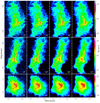 |
Fig. A.3 Column densities in the MHD simulation projected along the x axis (top), y axis (middle) and z axis (bottom) with the angular resolution indicated in the panels, overlaid with half-maximum ellipses representing the bound sources extracted by getsf. The linear scales, corresponding to the resolutions, are 0.07, 0.15, 0.31, and 0.62 pc. |
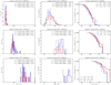 |
Fig. A.4 Same as in Fig. 8, but for the angular resolutions of 9′′ (top), 36′′ (middle row), and 72′′ (bottom). |
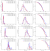 |
Fig. A.5 Same as Fig. A.4, but for the HDh model at 9′′ (top), 18′′ (second row), 36′′ (third row), and 72′′ (bottom). |
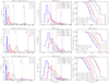 |
Fig. A.7 Effects of different angular resolutions on the sizes and masses of the bound sources in the simulated star-forming regions HD (top), MHD (middle row), and HDh (bottom). We show the source size function (left), the source mass function (middle), and the cumulative mass function (right), obtained for the x projection of the respective surface density maps. The other projections on the y and z directions are displayed in Figs. 7 and A.8. |
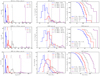 |
Fig. A.8 Effects of different angular resolutions on the sizes and masses of the bound sources in the simulated star-forming regions HD (top), MHD (middle row), and HDh (bottom). We show the source size function (left), the source mass function (middle), and the cumulative mass function (right), obtained for the z projection of the respective surface density maps. The other projections on the x and y directions are displayed in Figs. 7 and A.7. |
References
- Alves, J., Lombardi, M., & Lada, C. J. 2007, A&A, 462, L17 [NASA ADS] [CrossRef] [EDP Sciences] [Google Scholar]
- André, P., Men’shchikov, A., Bontemps, S., et al. 2010, A&A, 518, L102 [NASA ADS] [CrossRef] [EDP Sciences] [Google Scholar]
- André, P., Di Francesco, J., Ward-Thompson, D., et al. 2014, in Protostars and Planets VI, eds. H. Beuther, R. S. Klessen, C. P. Dullemond, & T. Henning (Tucson: University of Arizona Press), 27 [Google Scholar]
- André, P., Arzoumanian, D., Könyves, V., Shimajiri, Y., & Palmeirim, P. 2019, A&A, 629, L4 [CrossRef] [EDP Sciences] [Google Scholar]
- Arzoumanian, D., André, P., Didelon, P., et al. 2011, A&A, 529, L6 [CrossRef] [EDP Sciences] [Google Scholar]
- Arzoumanian, D., André, P., Könyves, V., et al. 2019, A&A, 621, A42 [NASA ADS] [CrossRef] [EDP Sciences] [Google Scholar]
- Bastian, N., Covey, K. R., & Meyer, M. R. 2010, ARA&A, 48, 339 [NASA ADS] [CrossRef] [Google Scholar]
- Berry, D. S. 2015, Astron. Comput., 10, 22 [NASA ADS] [CrossRef] [Google Scholar]
- Bleuler, A., & Teyssier, R. 2014, MNRAS, 445, 4015 [Google Scholar]
- Bontemps, S., Motte, F., Csengeri, T., & Schneider, N. 2010, A&A, 524, A18 [NASA ADS] [CrossRef] [EDP Sciences] [Google Scholar]
- Carral, P., Kurtz, S. E., Rodríguez, L. F., et al. 2002, AJ, 123, 2574 [NASA ADS] [CrossRef] [Google Scholar]
- Cheng, Y., Tan, J. C., Liu, M., et al. 2018, ApJ, 853, 160 [NASA ADS] [CrossRef] [Google Scholar]
- Federrath, C., & Banerjee, S. 2015, MNRAS, 448, 3297 [NASA ADS] [CrossRef] [Google Scholar]
- Fromang, S., Hennebelle, P., & Teyssier, R. 2006, A&A, 457, 371 [NASA ADS] [CrossRef] [EDP Sciences] [Google Scholar]
- Hennebelle, P. 2013, A&A, 556, A153 [NASA ADS] [CrossRef] [EDP Sciences] [Google Scholar]
- Hennebelle, P. 2018, A&A, 611, A24 [NASA ADS] [CrossRef] [EDP Sciences] [Google Scholar]
- Hennebelle, P., & Chabrier, G. 2008, ApJ, 684, 395 [NASA ADS] [CrossRef] [Google Scholar]
- Hopkins, P. F. 2012, MNRAS, 423, 2037 [NASA ADS] [CrossRef] [Google Scholar]
- Kirk, J. M., Ward-Thompson, D., Palmeirim, P., et al. 2013, MNRAS, 432, 1424 [NASA ADS] [CrossRef] [Google Scholar]
- Klessen, R. S. 2001, ApJ, 556, 837 [NASA ADS] [CrossRef] [Google Scholar]
- Kong, S. 2019, ApJ, 873, 31 [NASA ADS] [CrossRef] [Google Scholar]
- Könyves, V., André, P., Arzoumanian, D., et al. 2020, A&A, 635, A34 [CrossRef] [EDP Sciences] [Google Scholar]
- Könyves, V., André, P., Men’shchikov, A., et al. 2015, A&A, 584, A91 [NASA ADS] [CrossRef] [EDP Sciences] [Google Scholar]
- Kroupa, P. 2002, Science, 295, 82 [Google Scholar]
- Lada, C. J., & Lada, E. A. 2003, ARA&A, 41, 57 [NASA ADS] [CrossRef] [Google Scholar]
- Lee, Y.-N., & Hennebelle, P. 2018, A&A, 611, A89 [NASA ADS] [CrossRef] [EDP Sciences] [Google Scholar]
- Liu, M., Tan, J. C., Cheng, Y., & Kong, S. 2018, ApJ, 862, 105 [CrossRef] [Google Scholar]
- Lomax, O., Whitworth, A. P., Hubber, D. A., Stamatellos, D., & Walch, S. 2014, MNRAS, 439, 3039 [NASA ADS] [CrossRef] [Google Scholar]
- Loughran, L., McBreen, B., Fazio, G. G., et al. 1986, ApJ, 303, 629 [NASA ADS] [CrossRef] [Google Scholar]
- Louvet, F., Neupane, S., Garay, G., et al. 2019, A&A, 622, A99 [NASA ADS] [CrossRef] [EDP Sciences] [Google Scholar]
- Lu, J. R., Do, T., Ghez, A. M., et al. 2013, ApJ, 764, 155 [NASA ADS] [CrossRef] [Google Scholar]
- Massi, F., Weiss, A., Elia, D., et al. 2019, A&A, 628, A110 [EDP Sciences] [Google Scholar]
- Matthews, H. E., McCutcheon, W. H., Kirk, H., White, G. J., & Cohen, M. 2008, AJ, 136, 2083 [NASA ADS] [CrossRef] [Google Scholar]
- Men’shchikov, A. 2013, A&A, 560, A63 [NASA ADS] [CrossRef] [EDP Sciences] [Google Scholar]
- Men’shchikov, A. 2016, A&A, 593, A71 [NASA ADS] [CrossRef] [EDP Sciences] [Google Scholar]
- Men’shchikov, A. 2017, A&A, 607, A64 [NASA ADS] [CrossRef] [EDP Sciences] [Google Scholar]
- Men’shchikov, A. 2021, A&A, 649, A89 [EDP Sciences] [Google Scholar]
- Men’shchikov, A., André, P., Didelon, P., et al. 2012, A&A, 542, A81 [NASA ADS] [CrossRef] [EDP Sciences] [Google Scholar]
- Molinari, S., Schisano, E., Faustini, F., et al. 2011, A&A, 530, A133 [NASA ADS] [CrossRef] [EDP Sciences] [Google Scholar]
- Moser, E., Liu, M., Tan, J. C., et al. 2020, ApJ, 897, 136 [CrossRef] [Google Scholar]
- Motte, F., Andre, P., & Neri, R. 1998, A&A, 336, 150 [NASA ADS] [Google Scholar]
- Motte, F., Zavagno, A., Bontemps, S., et al. 2010, A&A, 518, L77 [NASA ADS] [CrossRef] [EDP Sciences] [Google Scholar]
- Motte, F., Nony, T., Louvet, F., et al. 2018, Nat. Astron., 2, 478 [NASA ADS] [CrossRef] [Google Scholar]
- Ntormousi, E., & Hennebelle, P. 2019, A&A, 625, A82 [EDP Sciences] [Google Scholar]
- Ntormousi, E., Hennebelle, P., André, P., & Masson, J. 2016, A&A, 589, A24 [NASA ADS] [CrossRef] [EDP Sciences] [Google Scholar]
- Ortiz-León, G. N., Dzib, S. A., Kounkel, M. A., et al. 2017, ApJ, 834, 143 [Google Scholar]
- Padoan, P., & Nordlund, Å. 2002, ApJ, 576, 870 [NASA ADS] [CrossRef] [Google Scholar]
- Padoan, P., Nordlund, A., & Jones, B. J. T. 1997, MNRAS, 288, 145 [NASA ADS] [CrossRef] [Google Scholar]
- Padoan, P., Nordlund, Å., Kritsuk, A. G., Norman, M. L., & Li, P. S. 2007, ApJ, 661, 972 [NASA ADS] [CrossRef] [Google Scholar]
- Pelkonen, V. M., Padoan, P., Haugbølle, T., & Nordlund, Å. 2021, MNRAS, 504, 1219 [NASA ADS] [CrossRef] [Google Scholar]
- Persi, P., & Tapia, M. 2008, ASP Monograph Pub., 5, 456 [NASA ADS] [Google Scholar]
- Rosolowsky, E. W., Pineda, J. E., Kauffmann, J., & Goodman, A. A. 2008, ApJ, 679, 1338 [NASA ADS] [CrossRef] [Google Scholar]
- Russeil, D., Zavagno, A., Adami, C., et al. 2012, A&A, 538, A142 [NASA ADS] [CrossRef] [EDP Sciences] [Google Scholar]
- Salpeter, E. E. 1955, ApJ, 121, 161 [Google Scholar]
- Sanhueza, P., Contreras, Y., Wu, B., et al. 2019, ApJ, 886, 102 [NASA ADS] [CrossRef] [Google Scholar]
- Schmidt, W., Kern, S. A. W., Federrath, C., & Klessen, R. S. 2010, A&A, 516, A25 [NASA ADS] [CrossRef] [EDP Sciences] [Google Scholar]
- Schneider, F. R. N., Sana, H., Evans, C. J., et al. 2018, Science, 359, 69 [NASA ADS] [CrossRef] [Google Scholar]
- Servajean, E., Garay, G., Rathborne, J., Contreras, Y., & Gomez, L. 2019, ApJ, 878, 146 [NASA ADS] [CrossRef] [Google Scholar]
- Smith, R. J., Clark, P. C., & Bonnell, I. A. 2009, MNRAS, 396, 830 [NASA ADS] [CrossRef] [Google Scholar]
- Smith, R. J., Glover, S. C. O., & Klessen, R. S. 2014, MNRAS, 445, 2900 [Google Scholar]
- Stutzki, J., & Guesten, R. 1990, ApJ, 356, 513 [NASA ADS] [CrossRef] [Google Scholar]
- Testi, L., & Sargent, A. I. 1998, ApJ, 508, L91 [NASA ADS] [CrossRef] [Google Scholar]
- Teyssier, R. 2002, A&A, 385, 337 [NASA ADS] [CrossRef] [EDP Sciences] [Google Scholar]
- Tigé, J., Motte, F., Russeil, D., et al. 2017, A&A, 602, A77 [NASA ADS] [CrossRef] [EDP Sciences] [Google Scholar]
- Tilley, D. A., & Pudritz, R. E. 2004, MNRAS, 353, 769 [NASA ADS] [CrossRef] [Google Scholar]
- Williams, J. P., de Geus, E. J., & Blitz, L. 1994, ApJ, 428, 693 [NASA ADS] [CrossRef] [Google Scholar]
- Willis, S., Marengo, M., Allen, L., et al. 2013, ApJ, 778, 96 [NASA ADS] [CrossRef] [Google Scholar]
- Zucker, C., Speagle, J. S., Schlafly, E. F., et al. 2020, A&A, 633, A51 [CrossRef] [EDP Sciences] [Google Scholar]
We adjusted the mass for a distance of 460 pc, while Bontemps et al. (2010) reported ≃3 × 10⁴ M⊙ for a source distant of 260 pc.
For brevity, we use the term ‘emission’, although we mostly discuss surface densities, not intensities. We also use the term ‘background’ to denote either structureless or filamentary background of sources.
Men’shchikov et al. (2012); Men’shchikov (2013, 2016, 2017, 2021) emphasise the background-related inaccuracies on the basis of the benchmark source extractions with getsources and getsf.
Dendrograms offers different ways to determine the source flux: either without background subtraction, or subtracting the value at the border of the source (default mode), or extrapolating the source profile down to the zero emission level.
All Tables
Source extractions in the observed and simulated regions at different angular resolutions.
All Figures
|
Fig. 1 Column densities of the high-mass star-forming region NGC 6334 (D ≃ 1750 pc). The imagesare overlaid with the half-maximum ellipses of the extracted bound sources (Sect. 3.1), with the angular resolutions indicated in each panel. The red rectangle in the left panel indicates the central region of NGC 6334 discussed in Sect. 4.1. |
| In the text | |
|
Fig. 2 Column densities of the low-mass star-forming region Aquila (D ≃ 460 pc). The images are overlaid with the half-maximum ellipses of the extracted bound sources (Sect. 3.1), with the angular resolutions indicated in each panel. |
| In the text | |
|
Fig. 3 Column densities obtained by projecting the HD simulation along the x axis, overlaid with the half-maximum ellipses of the extracted bound sources (Sect. 3.1). The angular resolutions, indicated in the panels, correspond to the linear scales of 0.07, 0.15, 0.3, and 0.6 pc. |
| In the text | |
|
Fig. 4 Surface densities obtained by projecting the HDh simulation along the x axis, overlaid with the half-maximum ellipses of the extracted bound sources (Sect. 3.1). The angular resolutions, indicated in the panels, correspond to linear scales of 0.02, 0.04, 0.08, and 0.16 pc. |
| In the text | |
|
Fig. 5 Each data point represents the ratio, R = F(2O)∕F(O), at the spatial resolutions O and 2O of either the number (top, F = NB) or mean mass (bottom, |
| In the text | |
|
Fig. 6 Effects of different angular resolutions on the derived sizes and masses of bound sources in the star-forming regions NGC 6334 (top) and Aquila (bottom). We show the source size function (left), the source mass function (middle), and the cumulative mass function (right). The dashed curves in the left panels are the lognormal fits to the source size distributions and the vertical lines indicate the median values for each distribution. The dashed lines in the right panels are the fits to the cumulative SMFs within the range 5− 50%. For NGC 6334 (resp. Aquila), these intervals correspond to 14–107 M⊙ (resp. 1–4) at 18′′, 54–418 M⊙ (resp. 2–11) at 36′′, and 323-1870 M⊙ (resp. 4–20) at 72′′. |
| In the text | |
|
Fig. 7 Effects of different angular resolutions on the sizes and masses of bound sources in the simulated star-forming regions HD (top), MHD (middle row), and HDh (bottom). We show the source size function (left), the source mass function (middle), and the cumulative mass function (right), obtained for the y projection of the respective column density maps. The other projections on the x and z directions are displayed in Figs. A.7 and A.8. The fits of the cumulative SMFs were done only for extractions with more than 40 bound sources. We fitted the cumulative SMFs in the mass range corresponding to 5–50% of the source samples; it corresponds to, from top to bottom: 40–128, 39–125, 5–19 M⊙ for the blue curves, 94–304, 76–329, 11–49 M⊙ for the red curves, 28–120 M⊙ for the grey curve, and 87–537 M⊙ for the purple curve. |
| In the text | |
|
Fig. 8 Derived size and mass functions of the bound cores extracted by getsf from the column densities at 18′′ resolution, obtained from the HD simulation along the x, y, and z axes. The vertical dashed lines indicate the median size or mass; the cumulative form of the mass functions were fit by power laws in the range of 5− 50%. |
| In the text | |
|
Fig. 9 Comparisons of the mass functions at 18′′ of the bound sources extracted by getsf in the star-forming regions NGC 6334 with those extracted in the HD (blue) and MHD (red) simulations. In case of NGC 6334, only the sources from the central region (red box in Fig. 1) were used. The numbers of sources were normalised to the peak of the mass function for NGC 6334 and the fits of the cumulative mass function were done within the range 10−50%. In all modelhistograms, the numbers of sources were averaged between the x, y, and z projections. |
| In the text | |
|
Fig. 10 Simple model explaining the angular resolution effects on the derived masses and sizes of the sources located on top of filaments or other background fluctuations. The model image, consisting of an unresolved source on top of a filament, was convolved to different resolutions using Gaussian beams (FWHM), indicated in the panels. Shown are the radial profiles of the model across the filament (left), the getsf -interpolated background of the source (middle), and the background-subtracted source (right). The true radial profile of the model source and filament is shown by the thick dotted line. The background was interpolated within a radius of 1.25 times the resolution, which fully encircles the true source convolved to the resolution. Derived mass of the background-subtracted source increases by the factors 1.08, 1.55, 2.45, 3.48, and 4.12, when degrading the resolution by a factor of two. At each resolution, the measured half-maximum size
|
| In the text | |
|
Fig. A.1 Column densities in the HD simulation projected along the y axis (top) and z axis (bottom), with the angular resolution indicated in the panels, overlaid with half-maximum ellipses representing the bound sources extracted by getsf. The density projection along the x axis is shown in Fig. 3. |
| In the text | |
|
Fig. A.2 Column densities in the HDh simulation projected along the y axis (top) and z axis (bottom), with the angular resolution indicated in the panels, overlaid with half-maximum ellipses representing the bound sources extracted by getsf. The density projection along the x axis isshown in Fig. 4. |
| In the text | |
|
Fig. A.3 Column densities in the MHD simulation projected along the x axis (top), y axis (middle) and z axis (bottom) with the angular resolution indicated in the panels, overlaid with half-maximum ellipses representing the bound sources extracted by getsf. The linear scales, corresponding to the resolutions, are 0.07, 0.15, 0.31, and 0.62 pc. |
| In the text | |
|
Fig. A.4 Same as in Fig. 8, but for the angular resolutions of 9′′ (top), 36′′ (middle row), and 72′′ (bottom). |
| In the text | |
|
Fig. A.5 Same as Fig. A.4, but for the HDh model at 9′′ (top), 18′′ (second row), 36′′ (third row), and 72′′ (bottom). |
| In the text | |
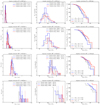 |
Fig. A.6 Same as Fig. A.5, but for the MHD model. |
| In the text | |
|
Fig. A.7 Effects of different angular resolutions on the sizes and masses of the bound sources in the simulated star-forming regions HD (top), MHD (middle row), and HDh (bottom). We show the source size function (left), the source mass function (middle), and the cumulative mass function (right), obtained for the x projection of the respective surface density maps. The other projections on the y and z directions are displayed in Figs. 7 and A.8. |
| In the text | |
|
Fig. A.8 Effects of different angular resolutions on the sizes and masses of the bound sources in the simulated star-forming regions HD (top), MHD (middle row), and HDh (bottom). We show the source size function (left), the source mass function (middle), and the cumulative mass function (right), obtained for the z projection of the respective surface density maps. The other projections on the x and y directions are displayed in Figs. 7 and A.7. |
| In the text | |
Current usage metrics show cumulative count of Article Views (full-text article views including HTML views, PDF and ePub downloads, according to the available data) and Abstracts Views on Vision4Press platform.
Data correspond to usage on the plateform after 2015. The current usage metrics is available 48-96 hours after online publication and is updated daily on week days.
Initial download of the metrics may take a while.