| Issue |
A&A
Volume 652, August 2021
|
|
|---|---|---|
| Article Number | A5 | |
| Number of page(s) | 18 | |
| Section | Extragalactic astronomy | |
| DOI | https://doi.org/10.1051/0004-6361/202140531 | |
| Published online | 30 July 2021 | |
A study of submillimeter methanol absorption toward PKS 1830−211:
Excitation, invariance of the proton-electron mass ratio, and systematics
1
Department of Space, Earth and Environment, Chalmers University of Technology, Onsala Space Observatory, 43992 Onsala, Sweden
e-mail: mullers@chalmers.se
2
Department of Physics and Astronomy, Vrije Universiteit, De Boelelaan 1081, 1081 HV Amsterdam, The Netherlands
3
Max-Planck-Institut für Radioastonomie, Auf dem Hügel 69, 53121 Bonn, Germany
4
Astron. Dept., King Abdulaziz University, PO Box 80203, Jeddah 21589, Saudi Arabia
5
National Centre for Radio Astrophysics, Tata Institute of Fundamental Research, Pune University, Pune 411007, India
Received:
10
February
2021
Accepted:
19
April
2021
Context. Methanol is an important tracer to probe physical and chemical conditions in the interstellar medium of galaxies. Methanol is also the most sensitive target molecule for probing potential space-time variations of the proton-electron mass ratio, μ, a dimensionless constant of nature.
Aims. We present an extensive study of the strongest submillimeter absorption lines of methanol (with rest frequencies between 300 and 520 GHz) in the z = 0.89 molecular absorber toward PKS 1830−211, the only high-redshift object in which methanol has been detected. Our goals are to constrain the excitation of the methanol lines and to investigate the cosmological invariance of μ based on their relative kinematics.
Methods. We observed 14 transitions of methanol, five of the A-form and nine of the E-form, and three transitions of A-13CH3OH, with ALMA. We analyzed the line profiles with a Gaussian fitting and constructed a global line profile that is able to match all observations after allowing for variations of the source covering factor, line opacity scaling, and relative bulk velocity offsets. We explore methanol excitation by running the non local thermal equilibrium radiative transfer code RADEX on a grid of kinetic temperatures and H2 volume densities.
Results. Methanol absorption is detected in only one of the two lines of sight (the southwest) to PKS 1830−211. There, the excitation analysis points to a cool (∼10 − 20 K) and dense (∼104 − 5 cm−3) methanol gas. Under these conditions, several methanol transitions become anti-inverted, with excitation temperatures below the temperature of the cosmic microwave background. In addition, we measure an abundance ratio A/E = 1.0 ± 0.1, an abundance ratio CH3OH/H2 ∼ 2 × 10⁻⁸, and a 12CH3OH/13CH3OH ratio 62 ± 3. Our analysis shows that the bulk velocities of the different transitions are primarily correlated with the observing epoch due to morphological changes in the background quasar’s emission. There is a weaker correlation between bulk velocities and the lower level energies of the transitions, which could be a signature of temperature-velocity gradients in the absorbing gas. As a result, we do not find evidence for variations of μ, and we estimate Δμ/μ=(−1.8 ± 1.2) × 10−7 at 1-σ from our multivariate linear regression.
Conclusions. We set a robust upper limit |Δμ/μ| < 3.6 × 10⁻⁷ (3σ) for the invariance of μ at a look-back time of half the present age of the Universe. Our analysis highlights that systematics need to be carefully taken into account in future radio molecular absorption studies aimed at testing Δμ/μ below the 10−7 horizon.
Key words: quasars: absorption lines / quasars: individual: PKS 1830−211 / galaxies: ISM / galaxies: abundances / ISM: molecules / radio lines: galaxies
© ESO 2021
1. Introduction
Methanol has a myriad of rotational transitions in the millimeter and submillimeter windows, many of which are commonly excited in the gas phase of the interstellar medium (ISM). It was first detected in space, toward the Galactic center, by Ball et al. (1970) using the 140-foot Green Bank telescope. The molecule is an asymmetric rotor1 and offers the possibility to determine both the kinetic temperature (Tkin) and the volume density (nH2) of molecular gas in the ISM; it is hence a powerful tool to probe physical conditions (e.g., Leurini et al. 2004). Methanol is thought to be formed on the surface of dust grains, and then released into the ISM after thermal or nonthermal desorption (see, e.g., van der Tak et al. 2000; Maret et al. 2005; Garrod et al. 2007). As a result, methanol emission is often associated with star-formation activity and shocks in the ISM. Methanol masers, in particular, have been used to classify the earliest phases in the process of massive star formation, depending on the excitation mechanisms at work (i.e., collisional excitation for class I methanol masers versus infrared pumping for class II masers: e.g., Batrla et al. 1987; Menten 1991). Nonthermal desorption, for example icy grain mantle sputtering by cosmic ray particles, can also release methanol into the gas phase in quiescent dark clouds (e.g., Dartois et al. 2020).
Methanol has been observed in a wide range of interstellar environments in the Milky Way, with typical abundances relative to H2 of 10−7 − 10−6 in hot molecular cores (see, e.g., Menten et al. 1988; Schilke et al. 2001, for Orion-KL) and 10−9 − 10−8 in cold dark and translucent interstellar clouds (e.g., Friberg et al. 1988; Walmsley et al. 1988; Turner 1998). On the other hand, it is not detected in the diffuse phase down to an abundance < 10−9 (Liszt et al. 2008). Furthermore, methanol has been detected by its thermal and maser emission in nearby galaxies (e.g., Henkel et al. 1987; Ellingsen et al. 2014; Humire et al. 2020), and also in absorption in NGC3079 (Impellizzeri et al. 2008) and in the z = 0.89 absorber toward PKS 1830−211 (Muller et al. 2011).
Methanol has a rich rotational spectrum of which the complexity reflects hindered internal rotation (torsional motion) of the OH radical group relative to the CH3 frame. Various dedicated studies have been carried out to determine accurate rest frequencies (see Xu et al. 2008 and references therein), and the BELGI program was developed for the analysis of the internally hindered rotation in combination with the asymmetric top structure (Hougen et al. 1994). The many methanol lines are documented in various molecular spectroscopy databases (e.g., the Cologne Database for Molecular Spectroscopy (CDMS): Müller et al. 2001, 2005; Endres et al. 2016, and the JPL catalog: Pickett et al. 1998).
Methanol exists in two different nuclear-spin states, depending on the net spin I of the three protons of the CH3 group. In A-type methanol (analogous to ortho-NH3), the proton spins are parallel to each other, and I = 3/2. In E-type methanol (analogous to para-NH3), one of the proton spins is antiparallel to the other two, and I = 1/2. Furthermore, E-type methanol has two degenerate forms (Lees 1973). Consequently, the relative statistical abundance ratio of A-type to E-type is not the ratio of the spin degeneracies (i.e., 2), but unity.
Spectroscopic observations of absorption lines toward high-redshift quasars can be used to test putative variations of the fundamental constants of physics on cosmological timescales (e.g., Savedoff 1956; Bahcall & Schmidt 1967; Uzan 2011). Such tests of Gyr-timescale evolution in constants like the fine structure constant α and the proton-electron mass ratio μ ≡ mp/me are complementary to laboratory-based studies using atomic clocks (e.g., Huntemann et al. 2014; Godun & Nisbet-Jones 2014; Safronova & Budker 2018), which probe changes on timescales of years. While a variety of observational approaches have been explored using different combinations of spectral lines (e.g., Thompson 1975; Varshalovich & Levshakov 1993; Dzuba et al. 1999; Chengalur & Kanekar 2003; Kanekar et al. 2004; Flambaum & Kozlov 2007; Jansen et al. 2011a), they all consist of comparing the inferred redshift of an object as measured from different spectral lines whose frequencies have different dependencies (sensitivity coefficients) on the constant or constants of interest. For example, if the proton-electron mass ratio at the absorption redshift is different from its laboratory value today by Δμ, then two lines with different sensitivity coefficients Kμ to a variation of μ would be observed to show a velocity (equivalently, redshift) offset Δv given by
The hydrogen molecule (H2) is the most abundant molecular species in the Universe and its ultraviolet transitions have long been used to probe μ-variation in absorbers towards high-redshift quasars (Thompson 1975; Varshalovich & Levshakov 1993). H2 has a strong-dipole absorption spectrum shifted to the optical domain for high-redshift objects (e.g., Malec & Buning 2010; van Weerdenburg & Murphy 2011). In view of the fact that electronic transitions are probed, the sensitivity coefficients are small with typical spreads of ΔKμ = 0.06 (Varshalovich & Levshakov 1993; Ubachs et al. 2007). The combined analysis of ten quasar systems with typically some 100 observable spectral lines, including lines pertaining to the HD isotopologue, has produced a constraint of |Δμ/μ| < 5 × 10⁻⁶ (at 3σ) for redshifts in the range z = 2.0 − 4.2 (Ubachs et al. 2016). However, it has been shown that systematic errors arising from the wavelength calibration of optical echelle spectrographs may limit the accuracy of such H2-based measurements of μ-variation (e.g., Griest et al. 2010; Rahmani et al. 2013; Whitmore & Murphy 2015).
Molecules that undergo quantum-tunneling motions in their electronic ground state exhibit much larger sensitivity coefficients than those of the H2 electronic transitions, and therefore they offer more appealing alternatives to search for μ-variation on cosmological timescales. One such molecule is ammonia, which has inversion lines with large sensitivity coefficients Kμ = −4.46 (Flambaum & Kozlov 2007). However, these lines come with the disadvantage of all having the same Kμ sensitivity. Therefore, they have to be used in combination with, e.g., pure rotational lines of other species, exhibiting Kμ = −1, to constrain Δμ/μ. This approach has been used to compare NH3 inversion lines to HCN and HCO+ lines (at zabs = 0.68 toward the quasar B 0218+357; Murphy et al. 2008), to HC3N lines (at zabs = 0.89, toward the quasar PKS 1830−211; Henkel et al. 2009), and to CS and H2CO lines (again at zabs = 0.68 toward B 0218+357; Kanekar 2011). From these studies, the best current (3σ) upper limits are |Δμ/μ| < 3.6 × 10⁻⁷ from z = 0.68 to today, and |Δμ/μ| < 1 × 10⁻⁶ from z = 0.89 to today, the latter corresponding to a look-back time of about half the present age of the Universe. However, comparing the redshifts of lines from different molecular species introduces the potential problem of chemical (and kinematic) segregation within the molecular cloud, resulting in possible systematic errors in these analyses.
The above systematic uncertainties may be removed by using spectral lines of a single molecular species that (i) have transitions with different sensitivity coefficients Kμ; (ii) have Kμ larger than for H2 and possibly as high as for NH3, or even higher; (iii) are relatively abundant in the ISM; and (iv) are easy to observe with a sufficient signal-to-noise ratio (S/N), even in cosmological sources. At present, two species, hydroxyl (OH) and methanol (CH3OH), satisfy all the above criteria; however, the OH Λ-doubled line frequencies depend on both α and μ, and hence cannot be used to probe changes in μ alone (Chengalur & Kanekar 2003). In the case of methanol, whose line frequencies depend on μ alone, the extreme μ-sensitivity is connected to the quantum tunneling of the OH-group through the threefold internal barrier spanned by the CH3 group. The spread in sensitivity coefficients, Kμ, calculated by Jansen et al. (2011a,b) and Levshakov et al. (2011), is up to several orders of magnitude larger than for H2, and in some cases, larger than the ΔKμ between inversion lines of NH3 and other rotational lines. These features make methanol the most sensitive probe of μ-variation among known interstellar molecules.
While methanol is abundant in the ISM and has already been the target of studies probing spatial variations in μ in the Milky Way (Levshakov et al. 2011; Ellingsen et al. 2011; Daprà et al. 2017), the molecular absorber at z = 0.89 toward PKS 1830−211 is currently the only object at cosmological distances in which methanol has been detected (Muller et al. 2011). The methanol lines in PKS 1830−211 have hence been used by a number of later works to probe cosmological evolution in μ (Ellingsen et al. 2012; Bagdonaite & Jansen 2013a; Bagdonaite et al. 2013b; Kanekar et al. 2015). Indeed, this absorber has yielded the most stringent constraint on changes in any constant on Gyr timescales, |Δμ/μ| < 6 × 10⁻⁷ (at 3σ significance; Kanekar et al. 2015), over ∼7.5 Gyr.
PKS 1830−211, at a redshift z = 2.5 (Lidman et al. 1999), is a blazar that is strongly lensed by an intervening galaxy at z = 0.89 (Wiklind & Combes 1996), which appears as a weak, nearly face-on spiral in a 814 Å image made with the Hubble Space Telescope (Winn et al. 2002). At millimeter wavelengths, the blazar emission is dominated by two bright and compact images (Frye et al. 1997; Muller et al. 2020b) separated by ∼1″, hereafter the northeast and southwest images. At centimeter wavelengths, the two images are embedded in a nearly complete Einstein ring (Subrahmanyan et al. 1990; Jauncey et al. 1991; Nair et al. 1993). The Einstein ring and compact images have different spectral indices, such that PKS 1830−211’s morphology gradually changes with frequency. The blazar is active throughout the electromagnetic spectrum, for example at millimeter and submillimeter wavelengths (e.g., Martí-Vidal et al. 2013, 2020; Martí-Vidal & Muller 2019), in the radio-centimeter domain (e.g., Jin et al. 2003; Allison et al. 2017), and in gamma rays (e.g., Abdo et al. 2015).
The molecular gas in the z = 0.89 lensing galaxy causes a remarkable absorption spectrum, with more than 60 species detected to date in the line of sight to the southwest image of PKS 1830−211 (e.g., Muller et al. 2011, 2014a; Tercero et al. 2020), including methanol (Muller et al. 2011; Bagdonaite & Jansen 2013a). The continuum emission associated with the southwest image has a size of only a fraction of a milli-arcsecond at millimeter wavelengths (Guirado et al. 1999), corresponding to a pencil-beam illumination of the order of ≲1 parsec in the plane of the z = 0.89 absorber. This, along with the intrinsic activity of the blazar, the geometry of the system (with the blazar’s jet pointed almost exactly in our direction), and the magnification due to gravitational lensing, leads to very special conditions that are conducive to temporal variations of the molecular absorption spectra in the millimeter domain (Muller & Guélin 2008; Schulz et al. 2015). This effect prevents the robust kinematical comparison of spectra obtained at widely different epochs and hampers studies to constrain μ-variations (Bagdonaite et al. 2013b). We note, however, that the spectra of H I and OH at radio-centimeter wavelengths have been remarkably stable for more than 20 years (Chengalur et al. 1999; Allison et al. 2017; Combes et al. 2021), perhaps due to the facts that the continuum illumination encompasses a much larger region here than at shorter wavelengths (due to the Einstein ring) and that the H I/OH gas exhibits a less clumpy distribution than observed for more complex molecules.
While temporal variations of the absorption profiles have been identified as the major systematics for constraining μ-invariance with methanol lines toward PKS 1830−211, there is also evidence for inhomogeneities in the absorbing gas, with temperature and density gradients (Sato et al. 2013; Bagdonaite et al. 2013b; Schulz et al. 2015; Muller et al. 2020a), possibly affecting the comparison of lines with different excitations. Therefore, such systematics also need to be addressed by new studies of μ variability. Attempts to spatially resolve the methanol absorption have been undertaken with long-baseline interferometry (Marshall et al. 2017), but with little success so far, due to severe limitations of sensitivity and dynamic range.
This aims of this work is a comprehensive study of the strongest submillimeter lines of methanol toward PKS 1830−211. The paper is divided into the following sections: observations are described in Sect. 2; overall results are given in Sect. 3; we analyze the line profile in Sect. 4; we constrain the excitation of the methanol gas in Sect. 5; and we investigate the invariance of μ in Sect. 6, with a particular attention given to systematics. A summary is given in Sect. 7.
2. Observations
The observations were performed with the Atacama Large Millimeter/submillimeter Array (ALMA) between 2019 July and August (ALMA project code 2018.1.00051.S.) and are summarized in Table 1.
Summary of the observations.
In 2019 July, a total of four different tunings were observed, in bands 4 (B4, ∼150 GHz), 5 (B5, ∼180 GHz), 6 (B6, ∼230 GHz), and 7 (B7, ∼280 GHz), to cover all the targeted redshifted methanol lines. During this time, the array was in extended configurations, with the longest baselines up to 8–14 km providing synthesized beams between 30 and 60 mas. The B4 and B6 tunings were observed close together in time, on July 10 and 11. The B5 and B7 tunings were observed consecutively on July 28. The B4 tuning was reobserved with exactly the same setup on 2019 August 17 to allow us to test potential temporal variations of the absorption profile over the duration of our observational campaign. At this time, the array was in a more compact configuration, with a maximum baseline < 4 km, yielding a synthesized beam of 0.18″.
For the B5, B6, and B7 tunings, the correlator was configured to cover four spectral windows, each of 1.875 GHz in width and with a spectral resolution of ∼1 MHz (after Hanning smoothing). For the B4 tuning, we configured three spectral windows of 0.9375 GHz with a narrower resolution of 0.56 MHz, while the remaining fourth spectral window, not covering any methanol lines, was set with a width of 1.875 GHz and a resolution of ∼1 MHz. The resulting velocity resolutions are in the range 1.0–1.6 km s−1 after Hanning smoothing, for all methanol lines. The observational details are summarized in Table 1.
The data calibration was done within the CASA2 package, following standard procedures. The bandpass responses of the antennas were determined from observations of the bright quasar J 1924−2914, which was also used to calibrate the flux density scale. According to ALMA observatory flux monitoring data, we expect a flux scale accuracy better than 5% at bands 4, 5, and 6, and better than 10% at band 7.
After the standard gain calibration using the quasar J 1832−2039, the phase solutions were further self-calibrated on the continuum of PKS 1830−211, applying phase-only gain corrections to every 6 s integration. Spectra were converted from the topocentric to LSRK3 reference frame with the CASA task mstransform. The conversion between LSRK and the heliocentric frame, which we chose as the velocity reference for easier comparison with previous work, is vHelio = vLSRK − 12.4 km s−1. The final spectra were extracted using the CASA-Python task UVMultiFit (Martí-Vidal et al. 2014), by fitting a model of two point sources (corresponding to the northeast and southwest core images of PKS 1830−211) to the interferometric visibilities.
We note that the third lensed image of PKS 1830−211, located about half-way between the northeast and southwest images with a flux density roughly 140 times weaker than that of the northeast source, as well as the weak extensions from the northeast and southwest images, are all detected from this same ALMA dataset (Muller et al. 2020b). However, these have a negligible effect on the absorption spectra extracted with a two point-source model and have hence been ignored here.
3. Results
3.1. Description of the spectra
The absorption profiles of the methanol lines that we detected toward the southwest image of PKS 1830−211 are presented in Fig. 1, together with those of some other species. We detected five transitions from A-CH3OH and nine from the E-form. These transitions are indicated on the methanol A- and E-state energy diagrams in Fig. A.1 and their spectroscopic parameters are given in Table A.1. None of the methanol lines were detected in emission, implying an absence of inversion and maser effects in all measured transitions. The penultimate column of Table 1 lists the rms noise (normalized to the continuum level) for each band, at velocity resolutions of ∼1 − 1.6 km s−1.
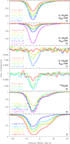 |
Fig. 1. ALMA spectra of methanol and several other species observed toward the southwest image of PKS 1830−211 during our campaign (July-August 2019). For lines in B4, the spectra were averaged over both B4a and B4b observations (see Fig. 3 for time variability). To avoid crowded plots and large spreads in absorption depths, the lines from A-CH3OH (a), E-CH3OH (b,c), and 13CH3OH (d) are separated, and they are also split according to low-level energy Elow < 30 K (b) and Elow > 30 K (c) for E-CH3OH. For comparison, some other species are shown in (e), for intermediate opacity lines, and (f), for lines with the highest opacity. |
At first glance, all methanol lines seem to have similar profiles, scaled by the respective line absorption strengths. The deepest absorption comes from the ground state transitions 11 − 00 of A-CH3OH and 2−2 − 1−1 of E-CH3OH, reaching an absorption depth of nearly 50% of the continuum level. The weakest detected transition, 6−2 − 6−1 E, has a lower-level energy Elow = 54 K with respect to the ground state of A-CH3OH, which is 7.90 K lower than that of E-CH3OH. The next E-CH3OH transition, 7−2 − 7−1 E with Elow = 70 K, is not detected, with an rms noise level of 1.1 × 10⁻³ of the continuum level. Among the observed A-CH3OH transitions, none has Elow higher than 30 K.
Except for the 21 − 10 A transition (rest frequency of 398.446920 GHz, redshifted to ∼211 GHz, which we skipped to limit the number of tunings and observing time, and because it has properties redundant with those of other targeted lines in terms of Elow and Kμ), we expect our survey of the methanol lines in the z = 0.89 absorber to be complete down to a peak opacity τ = 0.1 across all current ALMA bands (bands 3 to 10).
We also detect, for the first time toward PKS 1830−211, three transitions of the 13CH3OH isotopologue (Fig. 1d). These transitions correspond to the same series J−1 − J0 with J = 1, 2, 3 as for the main 12CH3OH isotopologue in B4. We determine the 12CH3OH/13CH3OH ratio in Sect. 5.3.
As observed before (e.g., Muller et al. 2011, 2020a; Ellingsen et al. 2012; Bagdonaite et al. 2013b; Kanekar et al. 2015; Marshall et al. 2017), the methanol absorption has a main component peaking at a velocity4v ∼ −5 km s−1. The ALMA spectra clearly reveal an additional shallow absorption feature between v = +4 km s−1 and +10 km s−1, which reveals itself in the new data either because of the significantly higher S/N or temporal variations in the line profile. For the methanol lines, the absorption depth of this side component is not as deep, relative to the main component, as for transitions of  O, H2CO, and N2H+, observed simultaneously, although these species have similar or even lower depths near v = −5 km s−1 (Fig. 1e). This suggests a relative enhancement of methanol absorption in the v = −5 km s−1 component.
Among all species observed in this campaign, the HCO+ (4 − 3) line shows the deepest absorption (Fig. 1f), and we infer that its continuum-covering factor is larger than 90% for the v ∼ −5 km s−1 component. We discuss the methanol spectra further in Sect. 4, where we construct a global absorption profile for all methanol lines.
3.2. Time variability of the quasar and of the absorption lines
Our observing campaign was designed to allow us to address the time variability of PKS 1830−211 as a systematic. For this reason, we requested all observations be performed within the shortest possible time interval, depending on the dynamical scheduling constraints of ALMA. To assess potential temporal variations, we requested a second B4 tuning as the final observation of our campaign. In this section, we investigate the intrinsic variability of the quasar and the evolution of the line profile within the time span of our observations.
We note that PKS 1830−211 endured a period of strong radio and gamma flaring activity about three months before our observations but had returned to an apparent quiescent stage by the time of our campaign (see, e.g., Martí-Vidal et al. 2020; Abhir et al. 2021).
3.2.1. Quasar activity
We used the continuum data to infer the quasar activity during our ALMA campaign. The evolution of the flux densities and flux ratios of the two northeast and southwest lensed images is shown in Fig. 2. The flux variations of the two images are delayed in time by ∼20 − 30 days with northeast leading (see, e.g., Muller et al. 2020b and references therein), but our sparse data cannot place strong constraints on the time delay. Nevertheless, this is not critical for our study, and we used a time delay of 27 days to reconstruct the intrinsic light curve of the quasar. The spectral energy distribution in Fig. 2b indicates that the spectral index α (defined by the relationship F = F0 × (ν/ν0)α) is close to −0.7. Then, we reconstructed the light curve of the quasar’s northeast image (Fig. 2d) by taking the flux density points of the northeast image corrected for the spectral index, and those of the southwest image shifted in time and corrected for spectral index and the relative magnification factor. With those additional points, we see that it is difficult to imagine large flux variations over short periods of less than ∼10 days, and we thus assume that the light curve is smooth after the start of our observations. A relative magnification factor of 1.04 would minimize the flux dispersion of points between July 10 and 28, leaving only minor flux density variations during our ALMA campaign, of at most 5%. The flux ratios are within the 1–2 range of past measurements (e.g., van Ommen et al. 1995; Muller & Guélin 2008; Martí-Vidal et al. 2013, 2020; Martí-Vidal & Muller 2019).
 |
Fig. 2. Temporal variations of the continuum emission of PKS 1830−211. (a) Evolution of the flux density of the northeast (red) and southwest (blue) lensed images during our ALMA campaign. (b) Spectral energy distribution (the frequency axis is on a logarithmic scale) of the two images (i.e., same data points as for (a) but now displayed as function of frequency), with the best fit of a F = F0(ν/ν0)α relationship indicated in dotted lines for each image. (c) Evolution of the instantaneous flux ratio R(t) = FNE/FSW. (d) Reconstructed flux density history (normalized by a flux F = 2.87 Jy at a frequency of 150 GHz and adopting a spectral index α = −0.7). The filled black dots correspond to datapoints from the northeast image, while the empty circles correspond to that from the southwest image, delayed in time by 27 days and rescaled adopting a relative magnification factor of 1.04 between the two images. |
3.2.2. Variability of the absorption profile
Since we reobserved the same tuning (B4) about one month apart, at the beginning and end of our methanol campaign, we were able to investigate the variability of the absorption profile of the different observed species. The difference spectra are shown in Fig. 3 for lines of CH3OH, N2H+, H2CO, and CH2NH. The profiles are in excellent agreement, except for a Gaussian-like feature in the difference spectra, at a velocity of −7.5 km s−1 and with a full width at half maximum (FWHM) of ∼6 km s−1 (i.e., in the blue wing of the main v = −5 km s−1 velocity component), which is common to all species. This feature corresponds to a change in integrated opacity within the velocity range −13 km s−1 to −2 km s−1 of less than 10%.
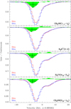 |
Fig. 3. Spectra of lines from CH3OH, N2H+, H2CO, and CH2NH, observed simultaneously on 2019 July 10 (B4a, in red) and August 17 (B4b, in blue). The difference spectra (B4b–B4a) are shown in green, multiplied by a factor two and shifted to unity. The best Gaussian fit to each of the difference spectra is overlaid as a dotted line, the cross indicating the velocity centroid, amplitude, and full-width at half maximum of the Gaussian. |
Such a variation, limited to a short range of velocities, shows evidence of small-scale and short-timescale structural changes in the morphology of the quasar5, and suggests as well that the different velocity components are likely to have different covering factors.
The peculiar variability of the main −5 km s−1 velocity component of the methanol absorption profile was already noticed by Muller et al. (2020a), with variations of a factor of two within a few months (between 2019 April and July). This, plus its chemical properties, led Muller et al. (2020a) to conclude that this velocity component may be associated with a compact dark cloud similar to those in the Milky Way.
3.3. Non-detection of methanol on the northeast line of sight
For completeness, we present the stacked spectrum corresponding to the weighted average of all A- and E-CH3OH transitions with Elow < 30 K toward the northeast image in Fig. A.2. Each observation was resampled to the same velocity grid with a velocity resolution δv = 2 km s−1 and we used the squared inverse of the rms noise levels in Table 1 as relative weights. The rms noise of the stacked spectrum is στ = 2.9 × 10⁻⁴ of the normalized continuum level with δv = 2 km s−1. Methanol remains undetected along this line of sight, which is known to contain more diffuse interstellar material than the southwest absorbing column (e.g., Muller et al. 2014b, 2017).
We calculated an upper limit of the methanol northeast column density from this non-detection. First, we determined the upper limit on the integrated opacity as  , where we assumed a line width Δv = 20 km s−1 for the absorption near v = −150 km s−1 (e.g., Muller et al. 2014a). For the ground-state transition of A-CH3OH (350.905 GHz rest frequency and one of the strongest absorption lines in our campaign), we calculated a conversion factor α = 2.2 × 1013 cm−2 km−1 s between integrated opacity and column density (Ncol = α∫τdv) under conditions of local thermodynamic equilibrium (LTE) with Tex = TCMB = 5.14 K. With a ratio A/E = 1, we then estimated a total methanol column density < 2.4 × 1011 cm−2 (3σ upper limit). With an H2 column density of 1 × 1021 cm−2 (Muller et al. 2014a), this upper limit corresponds to an abundance ratio CH3OH/H2 < 2.4 × 10⁻¹⁰, which is well below that in the southwestern line of sight (see Sect. 5.2) and consistent with the upper limit on methanol relative abundance in Galactic diffuse gas (< 10−9, Liszt et al. 2008).
4. Construction of a global line opacity profile for CH3OH
One of our main goals was to seek for potential velocity offsets between the different methanol lines in order to constrain the invariance of μ. We therefore need to adopt a model to compare the different transitions. A velocity centroid analysis would be a first order option, but one that is biased by the combined effects of the asymmetric absorption profile and opacity distortion of the spectra. Similarly, a cross-correlation analysis (e.g., similar to the approach followed by Kanekar et al. 2015) would not be suitable for the ALMA spectra since a number of the CH3OH lines of Fig. 1 are not optically thin. This is why we turned to a fit of a single common absorption profile, in terms of optical depths, to all methanol transitions toward the southwest image of PKS 1830−211.
We started our fitting exercise by forcing the background source covering factor (see Appendix B) fc = 1 for all spectra, but quickly realized that there were some tensions in the fit, as the deepest absorption could not be reproduced correctly and was systematically underestimated. Thus, we let fc be a free parameter. Although we see evidence for a varying fc across the absorption velocity interval, we adopted a constant fc as function of velocity because the temporal variations of the absorption profile have a small amplitude over the ∼1-month time span of our observations, and they are limited to a small range of velocities (Sect. 3.2.2). In addition, we wanted to minimize the complexity of the fit and number of fit parameters. However, we allowed fc to vary between the different tunings to account for potential variations with the observing epoch and frequency.
We chose to model the common line profile as a sum of Gaussian velocity components Gki with velocity centroids vk, FWHMΔvk, and integrated opacities ∫τdvk, scaled by an opacity factor γi and with a free bulk velocity vi for each transition i in a joint fit. Therefore, our model of the absorption profile Sj for all transitions i in tuning Bj, is described as follows:
![$$ \begin{aligned} S_j = 1 - f_{c}(B_j) \times \left[ 1- \exp { \left( - \sum _i \gamma _i \sum _{k} G_{ki} \right)} \right], \end{aligned} $$](/articles/aa/full_html/2021/08/aa40531-21/aa40531-21-eq4.gif)
where, in practice, we fixed the first Gaussian as G1i = G1(vi, Δv1, (∫τdv)1), to which we tied the next one as G2i = G2(vi + δv12, Δv2, (∫τdv)2), with δv12 the velocity separation between the first and second Gaussian. Hence, this velocity separation and the width and integrated area of each Gaussian component are forced to be constants for all lines through the fit. The vi and γi are free parameters for each line. We chose the ground-state transition of A-CH3OH (rest frequency 350.905 GHz, redshifted into band 5) as a reference for the normalization for the line profile (γ = 1), given that, as one of the brightest lines, it has a high S/N and it was observed roughly in the middle of our campaign. We checked that changing the reference line to another with comparable S/N did not change significantly the resulting covering factors and characteristics of the line profile.
For the fit, we used the Python scipy.optimize least-squares routine based on the Levenberg-Marquardt algorithm. The uncertainties are derived as the square root of the diagonal elements of the covariance matrix multiplied by the reduced χ2. Hence, we assume that errors follow a Gaussian distribution, that the parameters are not correlated, and that the model is a good representation of the data.
The best-fit parameters for the above model are given in Table 2, while the fits and residuals are shown in Fig. 4. The latter figure shows that all the lines are remarkably well reproduced with this minimal two-Gaussian model (reduced χ2 of 2.0 for 50 free parameters), with residuals below 1% of the continuum level and without any obvious features broader than a few km s−1. We therefore refrained from invoking a higher degree of complexity for the model by adding more velocity components.
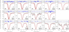 |
Fig. 4. Spectra of methanol transitions observed with ALMA toward the southwest image of PKS 1830−211, with best fits of the common two-Gaussian velocity component profile. The best fit is overlaid in red, and the fit residuals (data-model) are shown on top of each frame. The methanol form, quantum numbers (JK), and rest frequency (GHz) are given in the bottom right corner for each line. For B4 lines, the two visits are shown separately, with their respective fits. The ALMA band is given in the lower left corners. |
The methanol covering factors are in the 0.6–0.8 range, that is, smaller than fc previously measured toward PKS 1830−211 for any other species (e.g., Muller et al. 2014a), suggesting that methanol has a more compact distribution than other molecules. The change in fc between the two B4 tunings, at the start and end of our campaign, is ∼7%, which could indicate small morphological changes in PKS 1830−211. We find that, at a given time, fc is always increasing with frequency (i.e., fc(B4a) versus fc(B6), on one hand, and fc(B5) versus fc(B7), on the other hand). This could be interpreted as evidence of a smaller continuum size at higher frequency, for example due to a propagation effect in the ISM of the intervening galaxy (see, e.g., Guirado et al. 1999; Martí-Vidal et al. 2013). We refer the reader to Sect. 6.3 for a more detailed discussion of the covering factor and the interpretation of its frequency dependence. We also discuss the robustness of our fc fit measurements further in Appendix B.
5. Excitation of methanol lines
The physical conditions along the southwest line of sight to PKS 1830−211 have been investigated through multi-transition excitation studies using different species (Henkel et al. 2008; Muller et al. 2013), finding nH2 of the order of a few 103 cm−3 and Tkin ∼ 50 − 80 K, assuming the same physical conditions for the entire absorption profile. Under these conditions, the excitation of molecules with a high electric dipole moment (> 1 Debye) remains mostly coupled to the photons from the cosmic microwave background (TCMB = 5.14 K at z = 0.89)6. Nevertheless, there is growing evidence for chemical segregation between the different velocity components (e.g., Muller et al. 2011, 2016b, 2020a), potentially connected to different temperature and density conditions. In particular, the detection of deuterated species with large deuterium fractionation for the v = −5 km s−1 velocity component suggests a relatively cold gas temperature, < 30 K (Muller et al. 2020a), in contrast to the Tkin values given above.
In order to investigate the excitation of our methanol lines, we used the non-LTE radiative transfer code RADEX (van der Tak et al. 2007) with collisional rate coefficients from Pottage et al. (2004). These collisional rate coefficients were calculated for temperatures between 5 K and 200 K and rotational states up to J = 9. More recently, Rabli & Flower (2010) extended the rate calculations up to the level J = 15, although only for temperatures starting at 10 K. Para-H2 is assumed to be the main collisional partner, since it is expected to be the dominant form at low temperatures (T < 100 K). The background temperature was fixed to TCMB = 5.14 K, and we did not consider additional heating, either by the ambient radiative field or cosmic rays. We adopted a uniform sphere geometry and took the two-Gaussian line profile (i.e., fixing their velocity centroids, line widths, and integrated opacity ratios) and the covering factors determined in Table 2. We explored a density range between 103 and 106 cm−3 (in logarithmic steps) and kinetic temperatures between 6 and 100 K, varying also the G1 column density (that of G2 is tied by their integrated opacity ratio) and the A/E methanol abundance ratio. We note that the two velocity components are treated as if they were independent, given they are mostly kinematically decoupled, that is, radiative transfer issues were neglected. For each model, we constructed the RADEX methanol spectrum and calculated the resulting χ2, summing over the different tunings i as
where σi is the rms noise of the observations in tuning i. For this exercise, the two visits of the B4 tuning were averaged, and we took their average fc. The 13CH3OH transitions were also modeled, scaling the opacity of their corresponding 12CH3OH transition by a ratio of 62 (see Sect. 5.3), although they were not taken into account in the χ2 minimization.
The best-fit solution ( ) is found for column densities of A-CH3OH of 1.8 × 1014 cm−2 and 0.7 × 1014 cm−2 for G1 and G2, respectively, an A/E abundance ratio of 1, Tkin = 9 K, and nH2 = 1.3 × 105 cm−3. The corresponding RADEX model spectra are overlaid on the ALMA spectra in Fig. 5. It is not straightforward to define uncertainties in the four-dimensional parameter space. Nevertheless, in Fig. 6 we plot the reduced χ2 values obtained from the fit as a function of Tkin and nH2, after fixing the column densities of G1 and G2 to the above values, and A/E to unity. The equivalent 1σ contour, defined at a value Min
 , indicates a region with Tkin between 8 − 17 K and nH2 between 2 × 10⁴ − 2 × 105 cm−3, meaning a cold and dense methanol gas, although a solution with a higher temperature (Tkin > 20 K) and lower density (nH2 ≲ 104 cm−3) is not completely excluded. We note, a posteriori, that the Rayleigh-Jeans approximation (hν ≪ kBT) is not applicable for temperatures T ≲ 15 − 25 K for the submillimeter lines targeted here, preventing the use of the traditional rotation diagram analysis.
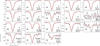 |
Fig. 5. RADEX excitation best-fit model (Tkin = 9 K, nH2 = 1.3 × 105 cm−3, A/E = 1, and Ncol(A) = 1.8 × 1014 cm−2 and 0.7 × 1014 cm−2 for the G1 and G2 velocity components in Table 2, respectively), overlaid in red on top of the ALMA methanol spectra toward the southwest image of PKS 1830−211. The methanol type, quantum numbers (JK), and rest frequency (GHz) are given in the bottom right corner for each transition. The ALMA band is given in the bottom left of each frame. The last row shows the 13CH3OH spectra (all of A type), with the RADEX fit of the corresponding transitions of the main isotopologue, scaled down by a factor 62; hence, these lines were not taken into account in the χ2 minimization. |
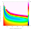 |
Fig. 6. Reduced χ2 results for the RADEX Tkin-nH2 grid search. The black contours are drawn at |


The match between the observed and RADEX spectra is remarkably good for transitions of A-CH3OH (Fig. 5, upper row). However, for most lines of E-CH3OH (except the ground state transition), the RADEX spectra underestimate the absorption depths. Removing the two lines with the largest mismatch from the  calculation, namely the 30 − 2−1 and 40 − 3−1 E lines, we obtained an improved value
  . This is a similar situation to that encountered by Daprà et al. (2017), who failed to reproduce the intensity of one of their E-CH3OH lines in the dark cloud L1498, in spite of its very simple cloud structure. We note that Daprà et al. (2017) used methanol collisional rates from Rabli & Flower (2010). We also explored solutions based on these rates, and found only minor improvements for few E-CH3OH lines, except the two lines mentioned above, which are still not well reproduced. On the other hand, we found some inconsistencies in the Aul Einstein coefficients in the LAMDA file of A-CH3OH associated with the Rabli & Flower (2010) rates, and for this reason, we continued to use the Pottage et al. (2004) rates for both A- and E-CH3OH.
We do not have a clear explanation for the above mismatch seen in a few lines. Possible paths for further investigations could be, for example, allowing different conditions between the A- and E-types, relaxing the single Tkin/nH2-set model to account for a multiphase medium, allowing different physical conditions and fc for the different velocity components, and considering collisions with ortho-H2 (Rabli & Flower 2010). All these would require more free parameters to fit, adding significant complexity to the problem, as well as additional inputs (the ortho-to-para ratio of H2, calculations of the corresponding rates, etc).
Finally, we note that according to our RADEX simulations, the excitation temperature of some lines of E-CH3OH are below TCMB. This does not impact the spectra simulated by RADEX, but it is an interesting curiosity, and we further discuss this anti-inversion effect in Appendix C.
5.1. The A/E ratio
From the results of our RADEX grid search, we estimate an abundance ratio A/E = 1.0 ± 0.1. This ratio corresponds to a nuclear spin temperature ≳20 K (see, e.g., Fig. 7 by Wirström et al. 2011). Since there are no allowed radiative or collisional transitions between A- and E-CH3OH species, the spin temperature should reflect the initial temperature at the formation stage of the molecule, unless other mechanisms in the ISM drive the population distribution toward the equilibrium ratio at high temperatures, A/E = 1 (see, e.g., Friberg et al. 1988). Observationally, the case is not clear (e.g., Wirström et al. 2011), and it is difficult to establish the processes of methanol formation based on the A/E ratio alone.
5.2. Methanol relative abundance
By adding the column densities of A- and E-CH3OH over the two velocity components G1 and G2, we estimate a total methanol column density of ∼5 × 1014 cm−2 along the southwest line of sight. We further take the H2 column density of 2 × 1022 cm−2, estimated by Muller et al. (2014a) using CH spectra (obtained in 2012), as an H2 proxy. This yields an average methanol abundance relative to H2 of CH3OH/H2 ∼ 2 × 10⁻⁸ toward the southwest image of PKS 1830−211. We note that this is a rough estimate, because there were some variations in the line profile between 2012 and 2019, and because the two velocity components G1 and G2 could have different molecular compositions. Nevertheless, this abundance falls between methanol abundances in Galactic cold dark clouds (∼10−9 − 10−8) and hot cores (≳10−7). We find a difference of at least two orders of magnitude for the CH3OH/H2 abundance ratio between the southwest and northeast lines of sight, clearly denoting their different chemical compositions (e.g., Muller et al. 2017, their Table 4).
5.3. The 12CH3OH/13CH3OH ratio
We detected absorption from three transitions of 13CH3OH (Fig. 1d), which are the counterparts of the three 12CH3OH transitions covered in the same B4 tuning. In the construction of the global line profile of the methanol absorption (Sect. 4), we tied the opacities of the 13CH3OH lines to those corresponding to the 12C- main isotopologue, considering only the two brightest ones, since the third one has a low S/N and falls close to the edge of the spectral window (see Fig. 1d). Accordingly, we determined a 12CH3OH/13CH3OH ratio of 62 ± 3. This value falls between the 12C/13C-isotopologue ratios ∼30 − 40, measured from HCO+, HCN, and HNC (Muller et al. 2006, 2011), and 97 ± 6 determined for CH+ (Muller et al. 2017), respectively. Therefore, this result suggests that fractionation effects play an important role and that a more detailed analysis (beyond the scope of this paper) will be necessary to derive the elemental 12C/13C ratio.
5.4. The nature of the v = −5 km s−1 velocity component
With the new estimate of physical conditions from methanol excitation, there is growing evidence that the v = −5 km s−1 velocity component is associated with the analog of a Galactic cold dark cloud. Muller et al. (2020a) gave a list of arguments to this effect: (i) the strong deuterium fractionation of ND, NH2D, and HDO (up to 100 times larger than the primordial D/H ratio), pointing toward a temperature ≲30 K, which is consistent with the cool and dense solution determined above; (ii) the chemical composition, with relative enhancement of molecules typically associated with dense cores (e.g., CH3OH, HC3N, N2H+, SO2); (iii) the fast time variability suggesting a typical size of the order of 1 pc (Muller & Guélin 2008; Muller et al. 2020a); (iv) hints at temperature-velocity gradients suggesting the existence of substructures in the absorbing gas, which adds to the evidence of a multiphase absorbing gas column (Schulz et al. 2015; Muller et al. 2016a,b, 2017).
We note that, from their Very Long Baseline Interferometry (VLBI) imaging of the 12.2 GHz transition of methanol, Marshall et al. (2017) found a possible offset between the strongest absorption and the peak of the continuum emission, suggesting that the size of the absorbing material is in the range 1–10 pc. Therefore, there is hope that a direct measurement of the size of the methanol absorbing cloud could be possible with future observations.
It is interesting to compare our study of methanol absorption in the z = 0.89 absorber with that of methanol emission from the L1498 dark cloud in the Milky Way Taurus-Auriga complex by Daprà et al. (2017). They found comparable excitation conditions: Tkin = 6 ± 1 K and nH2 ∼ 3 × 105 cm−3, and A/E = 1.00 ± 0.15. On the other hand, the FWHM of the methanol emission in L1498 is much narrower, < 0.2 km s−1, suggesting a low degree of turbulence. At z = 0.89, the heating by CMB photons brings an additional 2.4 K and it is possible that the heating by cosmic rays is higher than in the surroundings of L1498. Indeed, Muller et al. (2016a) estimated a cosmic-ray ionization rate of atomic hydrogen ζH ∼ 3 × 10⁻¹⁵ s−1 along the southwest line of sight toward PKS 1830−211, which is slightly higher than in the Milky Way at a comparable galactocentric radius.
6. Invariance of μ and systematics
The primary goal of our ALMA methanol campaign was to test the possibility of cosmological evolution in the proton-electron mass ratio μ from z = 0.89 to today. For this, we targeted most of the strongest submillimeter methanol transitions, for which a high spectral resolution (ν/δν ∼ 3 × 10⁵) and a high S/N (≳500) could be obtained with the ALMA observations. Although the spread in Kμ is limited, ΔKμ ∼ 17, the high S/N, the short time span of the observations (all performed within < 40 days), and the limited frequency range (Δν/ν ∼ 0.6) make it possible to obtain a reliable constraint, addressing systematic issues. Such systematic effects arise from two aspects, the absorption lines themselves and the background source structure. The former includes temporal variations of the absorption profile (Muller & Guélin 2008; Muller et al. 2014a) and chemical or excitation segregation (gas covering factor, co-spatiality of species and lines with different excitation). The latter stems from the chromatic dependence of the background source morphology; for example, the effect of the Einstein ring at low radio frequencies (Kanekar et al. 2015; Combes et al. 2021), frequency-dependent size of the continuum emission (Guirado et al. 1999), and the core shift due to opacity effects along the jet (Martí-Vidal et al. 2013), which can result in a changing line of sight or covering factor at different frequencies. Some assessments of the above systematics have been discussed in earlier studies of μ-invariance using PKS 1830−211 (Bagdonaite et al. 2013b; Kanekar et al. 2015).
We note that the uncertainties on our vi measurements are, in some cases, of the same order as the methanol rest frequency uncertainties listed in the CDMS database. Those entries are the results of a global fit to the CH3OH rotational spectrum (Xu et al. 2008), based on a total of 24 600 measured frequencies. While adequate for most astronomy studies, they do not have the best possible accuracy that could be achieved in the lab. Actually, the post-fit error given in the CDMS (∼10 kHz for the submillimeter CH3OH lines considered here) is much smaller than the error of an individual measurement (i.e., 50 kHz, Xu et al. 2008). For 13CH3OH, the CDMS entries are based on the work of Xu & Lovas (1997), with rest frequency uncertainties of 50 kHz. In order to take the rest frequency uncertainties into account, we thus added them quadratically to the uncertainties of our vi measurements.
On the other hand, the hyperfine structure splitting of methanol lines (of the order of 10 kHz; see, e.g., Coudert et al. 2015; Lankhaar et al. 2016) is negligible compared to the width of methanol absorption toward PKS 1830−211 and also remains small compared to the uncertainties of our vi measurements (see also the discussion of methanol hyperfine structure and its relevance to μ-invariance determination by Daprà et al. 2017). Besides, Lankhaar et al. (2018) noticed that the methanol hyperfine structure could be impacted by the Zeeman effect in case of strong magnetic fields (> 30 mG, as they quote). Again, this effect is completely negligible, given the line widths of the absorption toward PKS 1830−211, the uncertainties in our vi fit measurements, and the expected magnetic fields in molecular clouds.
Following Eq. (1) and taking the bulk velocities vi in Table 2 at face value (including transitions of 13CH3OH), weighted by the inverse of their squared uncertainties (to which we quadratically added the rest frequency uncertainties), together with the corresponding Kμ (see Table A.1 and Appendix D), we obtained vi/c = (2.9 ± 3.1) × 10−7 × Kμ + ( − 4.64 ± 0.16)/c, with errors quoted at a 1σ confidence level (CL). This provides us with a first upper limit |Δμ/μ| < 9.4 × 10⁻⁷ at 3σ CL. However, the reduced chi-squared is high ( ), and we clearly see a systematic drift of ∼0.3 km s−1 between B4a and B4b visits (Fig. 7, lower left panel), as well as an apparent correlation between vi and the low-level energy (Fig. 7, lower row, third panel) which was already noticed by Bagdonaite et al. (2013b). Therefore, we further performed several multivariate regression analyses, taking the different systematic effects into account to improve the statistical description of our data.
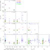 |
Fig. 7. Distribution matrix of relative bulk velocity offsets (δv), low-level energies (Elow), proton-electron sensitivity coefficients (Kμ), sky frequencies, and observation epochs, for observed methanol lines (Tables 2 and A.1). The Pearson r coefficients of the correlation matrix are given between the different variables. The data points corresponding to A-CH3OH and E-CH3OH transitions are marked with red crosses and blue squares, respectively. Those of 13CH3OH are indicated with green circles. The best results of the multivariate linear regression fit between the vi, time, Elow, and Kμ (see Table 3) are shown in the corresponding panels. |
The different possible variables to check for systematic effects are the observing epoch, the frequency, and the lower level energy of the transitions. Their correlation matrix is shown in Fig. 7. We did not consider the frequency and Kμ as simultaneous variables, because there is a clear correlation between them, with a Pearson coefficient r ∼ 0.8 (see also Jansen et al. 2011a). All other pairs of variables do not show significant correlation, with |r|≲0.4. The results of our different trials are given in Table 3, with different variable combinations for a multivariate linear regression analysis of the following type:

Best-fit parameters for the multivariate regression analysis of the vi measurements.
where Γt and ΓE are the coefficients of the correlation with time and Elow, respectively, and Γ0, a constant absorbing the velocity reference. Thus, Eq. (4) is a modified version of Eq. (1), with time and Elow systematics included.
Our first obvious result is that the fit quality drastically improves when a linear dependence with observing epoch is allowed, with  values decreasing from > 24 down to < 6. The correlation between vi and time is strong, with a coefficient |Γt|∼8 m s−1 d−1 determined at ∼10σ. We have further tested different time functions, such as quadratic polynomial and step functions, although the
  did not decrease drastically (
 ), while adding one more free parameter to fit when we only have three separated observing epochs. Thus we restrained ourselves to linear regression.
Besides the observing epoch, we found a weaker correlation between the vi and Elow, with a coefficient ΓE determined at 3σ at best. Replacing the Kμ by frequencies in Eq. (4), we did not find a significant correlation between vi and frequencies, showing that the chromatic effects from the background blazar have little impact on our constraint on Δμ/μ. Therefore, temporal variations of the absorption profile are the dominant systematic effect in our data.
Overall, the uncertainties on Δμ/μ do not change drastically throughout the different regressions, varying within the range (1.2 − 1.5) × 10−7 at 1σ CL once the vi shift with time is taken into account. The final multivariate regression with Kμ, observing epoch, and Elow yields the lowest  value (
 ) and gives the constraint Δμ/μ=(−1.8 ± 1.2) × 10−7 (1σ CL). Assuming a Gaussian distribution of errors, we take the 1-σ uncertainty8 of this fit result to obtain an upper limit of 3.6 × 10⁻⁷ at 3σ (99.7% CL) for |Δμ/μ| at a look-back time of half the present age of the Universe. Our results expand the study of Bagdonaite et al. (2013b) with a robust handling of the systematics, which we discuss in more detail in the following subsections.
It would be tempting to combine our ALMA observations of submillimeter methanol lines with other lines providing a large spread in ΔKμ, notably the 12.2 GHz transition which has a Kμ = −32, thus offering a large lever arm for constraints on Δμ/μ. This line was observed by several groups (Ellingsen et al. 2012; Bagdonaite & Jansen 2013a; Bagdonaite et al. 2013b; Kanekar et al. 2015; Marshall et al. 2017) between 2011 and 2013. The line centroid velocity is found to vary between −5 km s−1 and 0 km s−1 (with typical uncertainties of ∼1 km s−1) in fits with a single-Gaussian velocity component. The FWHM is found in the 8–20 km s−1 range. These differences may be due to temporal variations of the absorption profile (even if those are expected to be less than at millimeter wavelengths, Allison et al. 2017; Combes et al. 2021) or to the limited S/N of some of the observations. Furthermore, Kanekar et al. (2015), with the best S/N achieved on the 12.2 GHz line so far, made a detailed analysis of the 12.2, 48, and 60.5 GHz lines observed with the VLA between 2012 July and August. They showed that the 12.2 GHz line had a significantly different profile with respect to the two others, suggesting that it probes a different sightline. Hence, we remained conservative in our upper limit on Δμ/μ, and chose not to combine our results with previously published low-frequency methanol data.
6.1. Temporal variations of the absorption profile
The origin of the temporal variations of the vi, and of the absorption profile, is not clearly established, although it is most likely due to structural changes in the morphology of the quasar, possibly with the recurrent ejection of plasmons in the jet (Nair et al. 2005; Muller & Guélin 2008; Martí-Vidal et al. 2013; Schulz et al. 2015). The geometry of the system is indeed particularly favorable for such effects with the stretching due to a magnification factor of ∼3 (e.g., Muller et al. 2020b) and the blazar’s jet almost exactly oriented in our direction. In fact, evidence for superluminal motions was observed by Jin et al. (2003) during a monitoring of the relative separation between the two lensed images of PKS 1830−211 with VLBI. They found jumps in the plane of the sky of up to ∼200 μas within eight months, which would correspond to apparent motions at v ∼ 8c. Converted into the plane of the z = 0.89 absorber, such a motion would cover a projected distance of ∼1 pc in five months.
Within the same time interval of five months, the rate of change in velocity with time of Γt = 8 m s−1 d−1 obtained in our regression analysis would result in a velocity drift of ∼1 km s−1. If the cloud responsible of the methanol absorption is roughly placed on the size-line width relationship for Galactic molecular clouds (Larson 1981), it would have a line width of ∼1 km s−1 for a size of 1 pc. Therefore, the temporal variations observed in the line profile of methanol within a couple of months are naturally explained by superluminal motions in the continuum illumination, with the recurrent ejection of plasmons in the jet.
6.2. Temperature gradient
The correlation between line velocity and Elow was already noticed by Bagdonaite et al. (2013b; with the same sign, i.e., higher velocity toward higher Elow) and suggests a temperature gradient in the absorbing gas. Indeed, there is strong evidence of inhomogeneities along the southwest line of sight toward PKS 1830−211 (Sato et al. 2013; Schulz et al. 2015; Muller et al. 2016b, 2020a). The physical conditions were investigated by Henkel et al. (2008) and Muller et al. (2013), both finding a kinetic temperature of ∼50 − 80 K and an H2 density of ≈few × 103 cm−3 over the full line profile. If the two velocity components G1 and G2 have different physical properties (i.e., G1 being associated with a cold dark cloud, and G2 having a higher temperature), we would indeed expect a positive temperature gradient toward higher velocities.
6.3. Chromatic structure of the quasar
The morphology of PKS 1830−211 is highly dependent on the observing wavelength. The emission from the Einstein ring has a steep spectral index, and while it starts to become dominant at low radio frequencies (≲1 GHz), it is vanishingly weak in the millimeter and submillimeter domains (Muller et al. 2020b). There, almost all of the continuum emission arises from the two bright and compact core components, which have a spectral index of α ∼ −0.7, consistently with optically thin synchrotron emission (Fig. 2). The change in continuum illumination between centimeter and millimeter lines has a considerable effect on the resulting absorption profiles, as shown by Combes et al. (2021). However, the homogeneous set of millimeter-wave methanol lines is not expected to introduce a significant chromatic bias (e.g., by a differential illumination from the Einstein ring) in our study.
The sizes of the core images of PKS 1830−211 were measured at centimeter wavelengths, λ, with VLBI by Guirado et al. (1999). The angular size θ of the southwest image follows a steep θSW ∝ λ2 dependence, indicative of broadening due to interstellar scattering. In contrast, that of the northeast has a flatter dependence, θNE ∝ λ0.65, which Guirado et al. (1999) attributed to different scattering properties by interstellar plasma between the two lines of sight through the disk of the intervening galaxy. Extrapolating their measurements to the millimeter domain, we would obtain a size of the order of 1 μas for the southwest image. However, it is questionable whether the frequency-dependence of the size, which is established at radio-centimeter wavelengths, holds in the (sub)millimeter range, in which broadening by interstellar scattering is expected to have a far less significant effect.
If we interpret the covering factor fc as the ratio between the solid angle subtended by the absorbing gas to that of the continuum emission, fc = Ωgas/Ωcont, and if we assume that the absorbing gas has a constant solid angle, then the inverse of fc gives the solid angle subtended by the continuum emission in units of the solid angle subtended by the absorbing gas. In Fig. 8, we plotted 1/fc as a function of the observing frequency of our different visits. We estimate a rough relationship 1/fc ∝ ν−0.3, where the temporal variations of the continuum intensity largely dominate the error budget on the spectral index. The slope in this figure holds if we consider either the B4a–B6 pair or the B5–B7 pair separately. We thus find a much flatter size dependence on frequency at millimeter wavelengths than in the centimeter range. As an upper limit, the size of the southwest image in the millimeter range should be of the order of a tiny fraction of a milli-arcsecond. We note that the size of the continuum emission would only change by ∼20% over the frequencies covered by our campaign.
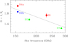 |
Fig. 8. Evolution of the inverse of the covering factor with frequency (both axes are on a logarithmic scale). The color-code indicates the observing epoch (red: 2019 Jul 10-11, green: 2019 Jul 28, and blue: 2019 Aug 17). |
Finally, we discuss the impact of a core-shift effect, which denotes a change of the core peak brightness location as a function of frequency, which is driven by opacity effects (see e.g., Marcaide & Shapiro 1984; Lobanov 1998). The shift θcs between two frequencies ν1 and ν2 can be expressed as
where Ω is the normalized core shift.
From early ALMA observations, Martí-Vidal et al. (2013) noticed the peculiar temporal and chromatic millimeter variability of the flux ratio between the two lensed images of PKS 1830−211, coincident in time with a strong gamma-ray flare. They proposed a simple model of plasmon ejection in the blazar’s jet to account for the ALMA observations and estimated a core shift of Ω ∼ 0.8 mas GHz, accounting for a magnification of three for the southwest image. Taking this value for the extreme frequencies of our ALMA campaign, we obtain a maximum core shift of ∼2 μas. Projected in the plane of the z = 0.89 absorber, this corresponds to a size of ∼0.02 pc, which is much smaller than the typical size of a molecular cloud, and not sufficient to introduce a significant correlation with frequency in our regression analysis.
In summary, the frequency-dependent morphology of the blazar can introduce strong biases in studies aiming to constrain μ-variations when comparing lines with a large difference in frequency (e.g., between the radio-centimeter and the millimeter and submillimeter windows). Nevertheless, all these chromatic effects remain small for the relatively narrow frequency range of our submillimeter line selection, and we did not see any significant correlation between the velocity measurements and the line frequencies.
6.4. Is there a difference between A/E methanol types?
A dependence of the line kinematics on the methanol type was suggested by Bagdonaite & Jansen (2013a) but later refuted by Bagdonaite et al. (2013b). Taking the same combinations as in Table 3 but separating A- and E-CH3OH in a new multivariate regression analysis, we did not see any significant differences in the resulting Γ coefficients between the two types. The constraint on Δμ/μ is slightly deteriorated, with 1σ uncertainties (1.5 − 1.8) × 10−7, depending on the adopted regression.
7. Summary and conclusions
We presented an absorption study of submillimeter lines of methanol from the z = 0.89 molecular absorber of the lensed blazar PKS 1830−211, with the goals of studying methanol excitation and probing cosmological evolution in the proton-electron mass ratio μ. Our main results are as follows:
-
we detected 14 methanol lines, five from A-CH3OH and nine from E-CH3OH, in absorption toward the southwest image of PKS 1830−211, as well as three transitions of 13CH3OH. None of the lines are detected in emission, implying that they are not affected by inversion, and thus do not amplify the background continuum.
-
Our excitation analysis points to a cool and dense methanol gas, with a kinetic temperature Tkin ∼ 10 − 20 K and a volume density nH2 ∼ 104 − 5 cm−2. We estimated a methanol abundance of ∼10−8 relative to H2. Such conditions are reminiscent of cold dark clouds in the Milky Way.
-
We determined a methanol A/E abundance ratio of 1.0 ± 0.1 and a 12CH3OH/13CH3OH ratio of 62 ± 3, the latter suggesting clear fractionation effects when compared to the 12C/13C-isotopologue ratios of other species.
-
We investigated the relative kinematics of the methanol lines in order to test for changes in μ. We found clear evidence that the absorption velocities of the different transitions depend on the observation epoch, probably due to temporal variations in the system. We also confirmed a correlation between the absorption velocities of the different lines and their lower energy levels, which we interpreted as a signature of a temperature gradient in the absorbing gas.
-
After taking these systematic effects into account by multivariate regression analysis, we did not find a significant correlation between the line bulk velocities and the Kμ sensitivity factors to variations in μ. We conclude that there is no evidence for changes in μ higher than |Δμ/μ| = 3.6 × 10⁻⁷ at 3σ confidence level, at a look-back time of ≈7.5 Gyr, which represents more than half the present age of the Universe.
This work illustrates the importance of addressing systematics effects to obtain a robust constraint on the cosmological invariance of fundamental constants. Future radio molecular absorption studies aimed at testing Δμ/μ below the 10−7 horizon, particularly those targeting PKS 1830−211, will have to be carefully designed.
Such changes have actually been observed with Very Long Baseline Interferometry (see e.g., Garrett et al. 1997).
The electric dipole moment of methanol is μa = 0.885 D for a−type transitions (with ΔK = 0) and μa = 1.44 D for b−type transitions (ΔK = ±1; Sastry et al. 1981).
The spread in Kμ with methanol transitions detected at centimeter wavelengths (e.g., by Ellingsen et al. 2012; Bagdonaite & Jansen 2013a; Bagdonaite et al. 2013b; Kanekar et al. 2015) can reach values of up to ∼30 (see Jansen et al. 2011a,b; Levshakov et al. 2011).
Acknowledgments
We thank the referee, Simon Ellingsen, for his constructive comments which improved the clarity of this work. This paper makes use of the following ALMA data: ADS/JAO.ALMA#2018.1.00051.S. ALMA is a partnership of ESO (representing its member states), NSF (USA) and NINS (Japan), together with NRC (Canada) and NSC and ASIAA (Taiwan) and KASI (Republic of Korea), in cooperation with the Republic of Chile. The Joint ALMA Observatory is operated by ESO, AUI/NRAO and NAOJ. This research has made use of NASA’s Astrophysics Data System. S. M. acknowledges support from Onsala Space Observatory for the provisioning of its facilities support. The Onsala Space Observatory national research infrastructure is funded through Swedish Research Council grant No 2017-00648.
References
- Abdo, A., Ackermann, M., Ajello, M., et al. 2015, ApJ, 799, 143 [Google Scholar]
- Abhir, J., Prince, R., Joseph, J., Bose, D., & Gupta, N. 2021, ApJ, 915, 26 [Google Scholar]
- Allison, J. R., Moss, V. A., Macquart, J.-P., et al. 2017, MNRAS, 465, 4450 [Google Scholar]
- Bahcall, J. N., & Schmidt, M. 1967, Phys. Rev. Lett., 19, 1294 [Google Scholar]
- Bagdonaite, J., Jansen, P., et al. 2013a, Science, 339, 46 [Google Scholar]
- Bagdonaite, J., Daprà, M., Jansen, P., et al. 2013b, Phys. Rev. Lett., 111, 231101 [Google Scholar]
- Ball, J. A., Gottlieb, C. A., Lilley, A. E., & Radford, H. E. 1970, ApJ, 162, 203 [Google Scholar]
- Batrla, W., Matthews, H. E., Menten, K. M., & Walmsley, C. M. 1987, Nature, 326, 49 [Google Scholar]
- Chengalur, J. N., de Bruyn, A. G., & Narasimha, D. 1999, A&A, 343, 79 [Google Scholar]
- Chengalur, J. N., & Kanekar, N. 2003, Phys. Rev. Lett., 91, 1302 [Google Scholar]
- Combes, F., Gupta, N., Muller, S., et al. 2021, A&A. A&A, 648, A116 [EDP Sciences] [Google Scholar]
- Coudert, L. H., Gutlé, C., Huet, T. R., et al. 2015, J. Chem. Phys., 143, 044304a [Google Scholar]
- Daprà, M., Henkel, C., Levshakov, S. A., et al. 2017, MNRAS, 472, 4434 [Google Scholar]
- Dartois, E., Chabot, M., Bacmann, A., et al. 2020, A&A, 634, A103 [NASA ADS] [CrossRef] [EDP Sciences] [Google Scholar]
- Dzuba, V. A., Flambaum, V. V., & Webb, J. K. 1999, Phys. Rev. Lett., 82, 888 [Google Scholar]
- Ellingsen, S., Voronkov, M., & Breen, S. 2011, Phys. Rev. Lett., 107, 270801 [Google Scholar]
- Ellingsen, S. P., Voronkov, M. A., Breen, S. L., & Lovell, J. E. J. 2012, ApJ, 747, L7 [Google Scholar]
- Ellingsen, S. P., Chen, X., Qiao, H.-H., et al. 2014, ApJ, 790, 28 [Google Scholar]
- Endres, C. P., Schlemmer, S., Schilke, P., Stutzki, J., & Müller, H. S. P. 2016, J. Mol. Spectr., 327, 95 [NASA ADS] [CrossRef] [Google Scholar]
- Flambaum, V. V., & Kozlov, M. G. 2007, Phys. Rev. Lett., 98, 240801 [NASA ADS] [CrossRef] [PubMed] [Google Scholar]
- Friberg, P., Madden, S. C., Hjalmarson, A., et al. 1988, A&A, 195, 281 [Google Scholar]
- Frye, B., Welch, W. J., & Broadhurst, T. 1997, ApJ, 478, 25 [Google Scholar]
- Garrett, M. A., Nair, S., Porcas, R. W., & Patnaik, A. R. 1997, Vistas Astron., 41, 281 [Google Scholar]
- Garrod, R. T., Wakelam, V., & Herbst, E. 2007, A&A, 467, 1103 [NASA ADS] [CrossRef] [EDP Sciences] [Google Scholar]
- Godun, R. M., Nisbet-Jones, P. B. R., et al. 2014, Phys. Rev. Lett., 113, 210801a [Google Scholar]
- Griest, K., Whitmore, J. B., Wolfe, A. M., et al. 2010, ApJ, 708, 158 [NASA ADS] [CrossRef] [Google Scholar]
- Guirado, J. C., Jones, D. L., Lara, L., et al. 1999, A&A, 346, 392 [NASA ADS] [Google Scholar]
- Henkel, C., Jacq, T., Mauersberger, R., Menten, K. M., & Steppe, H. 1987, A&A, 188, 1 [Google Scholar]
- Henkel, C., Braatz, J. A., Menten, K. M., & Ott, J. 2008, A&A, 485, 451 [NASA ADS] [CrossRef] [EDP Sciences] [Google Scholar]
- Henkel, C., Menten, K. M., Murphy, M. T., et al. 2009, A&A, 500, 725 [NASA ADS] [CrossRef] [EDP Sciences] [Google Scholar]
- Hougen, J. T., Kleiner, I., & Godefroid, M. 1994, J. Mol. Spectr., 163, 559 [Google Scholar]
- Humire, P. K., Henkel, C., & Gong, Y. 2020, A&A, 633, A106 [EDP Sciences] [Google Scholar]
- Huntemann, N., Lipphardt, B., Tamm, Chr., Gerginov, V., Weyers, S., & Peik, E. 2014, Phys. Rev. Lett., 113, 210802 [Google Scholar]
- Impellizzeri, C. M. V., Henkel, C., Roy, A. L., & Menten, K. M. 2008, A&A, 484, 43 [NASA ADS] [CrossRef] [EDP Sciences] [Google Scholar]
- Jansen, P., Xu, L.-H., Kleiner, I., Ubachs, W., & Bethlem, H. L. 2011a, Phys. Rev. Lett., 106, 100801 [Google Scholar]
- Jansen, P., Kleiner, I., Xu, L.-H., Ubachs, W., & Bethlem, H. L. 2011b, Phys. Rev. A, 84, 052509 [Google Scholar]
- Jauncey, D. L., Reynolds, J. E., Tzioumis, A. K., et al. 1991, Nature, 352, 132 [Google Scholar]
- Jin, C., Garrett, M. A., Nair, S., et al. 2003, MNRAS, 340, 1309 [Google Scholar]
- Kanekar, N. 2011, ApJ, 728, L12 [Google Scholar]
- Kanekar, N., Chengalur, J. N., & Ghosh, T. 2004, Phys. Rev. Lett., 93, 051302 [Google Scholar]
- Kanekar, N., Ubachs, W., Menten, K. M., et al. 2015, MNRAS, 448, 104 [Google Scholar]
- Lankhaar, B., Groenenboom, G. C., & van der Avoird, A. 2016, J. Chem. Phys., 145, 244301 [Google Scholar]
- Lankhaar, B., Vlemmings, W., Surcis, G., et al. 2018, Nat. Astron., 2, 145 [Google Scholar]
- Larson, R. B. 1981, MNRAS, 194, 809 [Google Scholar]
- Lees, R. M. 1973, ApJ, 184, 763 [Google Scholar]
- Leurini, S., Schilke, P., Menten, K. M., et al. 2004, A&A, 422, 573 [NASA ADS] [CrossRef] [EDP Sciences] [Google Scholar]
- Levshakov, S. A., Kozlov, M. G., & Reimers, D. 2011, ApJ, 738, 26 [Google Scholar]
- Lidman, C., Courbin, F., Meylan, G., et al. 1999, ApJ, 514, L57 [Google Scholar]
- Liszt, H. S., Pety, J., & Lucas, R. 2008, A&A, 486, 493 [NASA ADS] [CrossRef] [EDP Sciences] [Google Scholar]
- Lobanov, A. P. 1998, A&A, 330, 79 [NASA ADS] [Google Scholar]
- Malec, A. L., Buning, R., et al. 2010, MNRAS, 403, 1541 [Google Scholar]
- Marcaide, J. M., & Shapiro, I. I. 1984, ApJ, 276, 56 [Google Scholar]
- Maret, S., Ceccarelli, C., Tielens, A. G. G. M., et al. 2005, A&A, 442, 527 [NASA ADS] [CrossRef] [EDP Sciences] [Google Scholar]
- Marshall, M. A., Ellingsen, S. P., Lovell, J. E. J., et al. 2017, MNRAS, 466, 2450 [Google Scholar]
- Martí-Vidal, I., & Muller, S. 2019, A&A, 621, A18 [NASA ADS] [CrossRef] [EDP Sciences] [Google Scholar]
- Martí-Vidal, I., Muller, S., Combes, F., et al. 2013, A&A, 558, A123 [NASA ADS] [CrossRef] [EDP Sciences] [Google Scholar]
- Martí-Vidal, I., Vlemmings, W., Muller, S., & Casey, S. 2014, A&A, 563, A136 [NASA ADS] [CrossRef] [EDP Sciences] [Google Scholar]
- Martí-Vidal, I., Muller, S., Mus, A., et al. 2020, A&A, 638, A13 [CrossRef] [EDP Sciences] [Google Scholar]
- Menten, K. M. 1991, ApJ, 380, 75 [Google Scholar]
- Menten, K. M., Walmsley, C. M., Henkel, C., et al. 1988, A&A, 198, 253 [Google Scholar]
- Muller, S., & Guélin, M. 2008, A&A, 491, 739 [NASA ADS] [CrossRef] [EDP Sciences] [Google Scholar]
- Muller, S., Guélin, M., Dumke, M., et al. 2006, A&A, 458, 417 [NASA ADS] [CrossRef] [EDP Sciences] [Google Scholar]
- Muller, S., Beelen, A., Guélin, M., et al. 2011, A&A, 535, A103 [NASA ADS] [CrossRef] [EDP Sciences] [Google Scholar]
- Muller, S., Beelen, A., Black, J. H., et al. 2013, A&A, 551, A109 [NASA ADS] [CrossRef] [EDP Sciences] [Google Scholar]
- Muller, S., Combes, F., Guélin, M., et al. 2014a, A&A, 566, A112 [NASA ADS] [CrossRef] [EDP Sciences] [Google Scholar]
- Muller, S., Black, J. H., Guélin, M., et al. 2014b, A&A, 566, A6 [NASA ADS] [CrossRef] [EDP Sciences] [Google Scholar]
- Muller, S., Kawaguchi, K., Black, J. H., & Amano, T. 2016a, A&A, 589, A5 [EDP Sciences] [Google Scholar]
- Muller, S., Müller, H. S. P., Black, J. H., et al. 2016b, A&A, 595, A128 [NASA ADS] [CrossRef] [EDP Sciences] [Google Scholar]
- Muller, S., Müller, H. S. P., Black, J. H., et al. 2017, A&A, 606, A109 [NASA ADS] [CrossRef] [EDP Sciences] [Google Scholar]
- Muller, S., Jaswanth, S., Horellou, C., & Martí-Vidal, I. 2020a, A&A, 641, A2 [CrossRef] [EDP Sciences] [Google Scholar]
- Muller, S., Roueff, E., Black, J. H., et al. 2020b, A&A, 637, A7 [EDP Sciences] [Google Scholar]
- Müller, H. S. P., Thorwirth, S., Roth, D. A., & Winnewisser, G. 2001, A&A, 370, L49 [NASA ADS] [CrossRef] [EDP Sciences] [Google Scholar]
- Müller, H. S. P., Schlöder, F., Stutzki, J., & Winnewisser, G. 2005, J. Mol. Struct., 742, 215 [Google Scholar]
- Murphy, M. T., Flambaum, V. V., Muller, S., & Henkel, C. 2008, Science, 320, 1611 [Google Scholar]
- Nair, S., Narasimha, D., & Rao, A. P. 1993, ApJ, 407, 46 [Google Scholar]
- Nair, S., Jin, C., & Garrett, M. A. 2005, MNRAS, 362, 1157 [Google Scholar]
- Palmer, P., Zuckerman, B., Buhl, D., & Snyder, L. E. 1969, ApJ, 156, 147 [Google Scholar]
- Pandian, J. D., Leurini, S., Menten, K. M., Belloche, A., & Goldsmith, P. F. 2008, A&A, 489, 1175 [NASA ADS] [CrossRef] [EDP Sciences] [Google Scholar]
- Pickett, H. M., Poynter, R. L., Cohen, E. A., et al. 1998, J. Quant. Spectrosc. Rad. Transfer, 60, 883 [Google Scholar]
- Pottage, J. T., Flower, D. R., & Davis, S. L. 2004, MNRAS, 352, 39 [Google Scholar]
- Rabli, D., & Flower, D. R. 2010, MNRAS, 406, 95 [Google Scholar]
- Rahmani, H., Wendt, M., Srianand, R., et al. 2013, MNRAS, 435, 861 [NASA ADS] [CrossRef] [Google Scholar]
- Safronova, M. S., Budker, D., et al. 2018, Rev. Mod. Phys., 90, 025008 [Google Scholar]
- Sastry, K. V. L. N., Lees, R. M., & Van der Linde, J. 1981, J. Mol. Spectr., 88, 228 [Google Scholar]
- Sato, M., Reid, M. J., Menten, K. M., & Carilli, C. L. 2013, ApJ, 764, 132 [Google Scholar]
- Savedoff, M. P. 1956, Nature, 178, 688 [Google Scholar]
- Schilke, P., Benford, D. J., Hunter, T. R., Lis, D. C., & Phillips, T. G. 2001, ApJS, 132, 281 [Google Scholar]
- Schulz, A., Henkel, C., Menten, K. M., et al. 2015, A&A, 574, A108 [NASA ADS] [CrossRef] [EDP Sciences] [Google Scholar]
- Subrahmanyan, R., Narasimha, D., Pramesh-Rao, A., & Swarup, G. 1990, MNRAS, 246, 263 [Google Scholar]
- Tercero, B., Cernicharo, J., Cuadrado, S., de Vicente, P., & Guélin, M. 2020, A&A, 636, A7 [CrossRef] [EDP Sciences] [Google Scholar]
- Thompson, R. I. 1975, Astrophys. Lett., 16, 3 [NASA ADS] [Google Scholar]
- Turner, B. E. 1998, ApJ, 501, 731 [Google Scholar]
- Ubachs, W., Buning, R., Eikema, K. S. E., & Reinhold, E. 2007, J. Mol. Spectr., 241, 155 [Google Scholar]
- Ubachs, W., Bagdonaite, J., Salumbides, E. J., Murphy, M. T., & Kaper, L. 2016, Rev. Mod. Phys., 88, 021003 [Google Scholar]
- Uzan, J.-P. 2011, Liv. Rev. Rel., 14, 2 [Google Scholar]
- van der Tak, F. F. S., van Dishoeck, E. F., & Caselli, P. 2000, A&A, 361, 327 [NASA ADS] [Google Scholar]
- van der Tak, F. F. S., Black, J. H., Schöier, F. L., Jansen, D. J., & van Dishoeck, E. F. 2007, A&A, 468, 627 [NASA ADS] [CrossRef] [EDP Sciences] [Google Scholar]
- van Ommen, T. D., Jones, D. L., Preston, R. A., & Jauncey, D. L. 1995, ApJ, 444, 561 [Google Scholar]
- Varshalovich, D. A., & Levshakov, S. A. 1993, JETP Lett., 58, 237 [NASA ADS] [Google Scholar]
- van Weerdenburg, F., Murphy, M. T., et al. 2011, Phys. Rev. Lett., 106, 180802 [Google Scholar]
- Walmsley, C. M., Batrla, W., Matthews, H. E., & Menten, K. M. 1988, A&A, 197, 271 [Google Scholar]
- Whitmore, J. B., & Murphy, M. T. 2015, MNRAS, 447, 446 [NASA ADS] [CrossRef] [Google Scholar]
- Wiklind, T., & Combes, F. 1996, Nature, 379, 139 [Google Scholar]
- Winn, J. N., Kochanek, C. S., McLeod, B. A., et al. 2002, ApJ, 575, 103 [Google Scholar]
- Wirström, E. S., Geppert, W. D., Hjalmarson, A., et al. 2011, A&A, 533, A24 [NASA ADS] [CrossRef] [EDP Sciences] [Google Scholar]
- Xu, L.-H., & Lovas, F. J. 1997, J. Phys. Chem. Ref. Data, 26, 17 [Google Scholar]
- Xu, L.-H., Fisher, J., Lees, R. M., et al. 2008, J. Mol. Spectr., 251, 305 [NASA ADS] [CrossRef] [Google Scholar]
- Zeiger, B., & Darling, J. 2010, ApJ, 709, 386 [Google Scholar]
Appendix A: Additional information
The spectroscopic parameters of the submillimeter methanol lines observed in our campaign are given in Table A.1. Their energy levels are plotted in Fig. A.1 for A-CH3OH and E-CH3OH separately. We note that the ground state of E-CH3OH lies 7.90 K above that of A-CH3OH. The methanol spectra toward the northeast image of PKS 1830−211 are shown in Fig. A.2, together with their stacked spectrum and with the spectra of HCO+ and HCN J = 4 − 3 transitions.
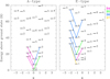 |
Fig. A.1. Energy level diagram for the lower transitions of A-type (left) and E-type (right) methanol. The quantum numbers are J, as marked on the right of each level in the diagram, and K, as given on the x-axis. The transitions observed by us are indicated by the lines, for which the color-code corresponds to the different tunings. We note that the ground state level of E-CH3OH lies 7.9 K above that of A-CH3OH. |
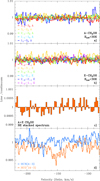 |
Fig. A.2. (a, b) ALMA spectra of A/E-CH3OH transitions observed toward the northeast image of PKS 1830−211. (c) Stacked spectrum, resulting from the weighted average of all A and E transitions with Elow < 30 K, regridded to a velocity resolution of 2 km s−1. (d) For reference: HCO+(4-3) and HCN(4-3) absorption spectra toward the northeast image. |
Spectroscopic parameters of methanol lines observed by us.
Appendix B: Covering factor
The covering factor, fc, is the geometrical parameter that describes how much the absorbing material covers the background illuminating source (Ibg). The absorption spectrum Iabs is connected to the opacity of the obscuring material via
![$$ \begin{aligned} I_{\rm abs} = I_{\rm bg} \times \left[ 1-{f_c} \times (1- \exp {(-\tau )}) \right]. \end{aligned} $$](/articles/aa/full_html/2021/08/aa40531-21/aa40531-21-eq22.gif)
It is easy to see that in the case of an optically thin line (τ ≪ 1):
and hence that there is an observational degeneracy between fc and the true opacity.
How can we determine fc? In the case of a heavily saturated line (τ ≫ 1), Iabs tends toward Ibg × (1 − fc), and fc can then be measured directly on the flat-bottom shape of the spectrum around the line center. For species with hyperfine structure that are spectrally resolved with a good S/N, fc and the true opacities can be determined under the assumption that the intensities of the different hyperfine components follow their statistical weights. When several lines with a spread in opacity are observed, then again, fc can be fit with the assumption of a common line profile, provided a good enough S/N of the data.
We note that in general, and in particular in the case of PKS 1830−211, fc could vary in time and frequency due to potential time evolution and chromatic morphology of the background source (see, e.g., Martí-Vidal et al. 2013), as well as with line excitation, in the case of temperature gradients in the absorbing gas.
Appendix C: Anomalous methanol absorption
In thermodynamic equilibrium, the relative population ni of the different energy levels Ei is described by the Boltzmann equation:
where u and l denote an upper and lower level, respectively, gi is the level degeneracy, kB, the Boltzmann constant, and Tex, the excitation temperature. Under some circumstances in the ISM, however, the level populations can deviate from their equilibrium values. For example, when external radiative (e.g., strong infrared field) or collisional (e.g., high density and high kinetic temperature) pumping occurs, the upper energy levels of some transitions may become overpopulated (nu/gu > nl/gl), the so-called population inversion, potentially triggering intense maser emission (e.g., for OH, H2O, and CH3OH molecules). On the other hand, in regions with low temperature dominated by collisional excitation, the populations of some levels may become anti-inverted, with overpopulation of the lower energy level, depending on the balance between collisional rates and radiative decays. The excitation temperature may even become lower than the CMB temperature, and the molecule would then be seen in absorption against the CMB. This was observed for formaldehyde lines (e.g., toward Galactic dark clouds, Palmer et al. 1969; see also Zeiger & Darling 2010, and their discussion regarding the z = 0.68 absorber toward B 0218+357) and also for methanol lines (e.g., Walmsley et al. 1988; Pandian et al. 2008).
In Fig. C.1, we show the evolution of the excitation temperature with volume density for all methanol transitions in our survey. At low density, nH2 ≲ 103 cm−3, Tex stays coupled to the CMB temperature (TCMB = 5.14 K at z = 0.89). At higher density, the collisions progressively raise Tex until it eventually converges to Tkin. However, for E-CH3OH, all the J−2 − J−1 transitions in our survey (J = 2–6) show a decrease of Tex below TCMB before they rise again beyond nH2 > 106 − 7 cm−3. Under these conditions, the lines would be seen in absorption against the CMB, even if there were no background quasar emission.
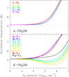 |
Fig. C.1. Evolution of the excitation temperature with the H2 density for methanol transitions in our survey, obtained from RADEX. We fixed a column density of 1 × 1014 cm−2, a FWHM of 1 km s−1, and a kinetic temperature of 10 K. The CMB temperature at z = 0.89 is marked by the dashed line. |
Using RADEX, we further searched for methanol transitions between 1 and 1000 GHz possibly showing a large anti-inversion effect. We set a column density of 1 × 1014 cm−2 for both A- and E-CH3OH, a FWHM of 1 km s−1, Tkin = 10 K, and we fixed nH2 = 3 × 105 cm−3, since it is in the density regime where lines in our survey present the largest negative difference between Tex and TCMB. From this first RADEX run, we selected the lines with ΔT = TCMB − Tex > 1 K and with peak opacity τ > 0.01. Fig. C.2 shows the evolution of Tex with nH2 for all these selected lines. We find the maximum anti-inversion for the 51 − 60 line of A-CH3OH, at a rest frequency of 6.7 GHz, for which Tex goes below 0.5 K for densities between 104 and 106 cm−3. It reaches Tex ∼ 0.25 K at its minimum. This line is associated with strong interstellar maser emission (Menten 1991), and it is thus prone to inversion or anti-inversion depending on the excitation conditions. As mentioned above, anti-inversion, leading to enhanced absorption, has indeed been observed in this line (Pandian et al. 2008). For E-CH3OH, the strongest anti-inversion is attained by the 20 − 3−1 line at rest frequency 12.2 GHz, first observed by Walmsley et al. (1988). It is also known as a strong masing line (Batrla et al. 1987). For this line, Tex drops to a minimum value of ∼1 K under the assumed physical conditions.
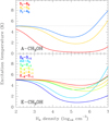 |
Fig. C.2. Evolution of the excitation temperature with the H2 density for methanol transitions harboring the maximum anti-inversion effect between 1 and 1000 GHz. The settings are the same as in Fig. C.1. The CMB temperature at z = 0.89 is marked by dashed lines. |
Appendix D: Kμ methanol sensitivity coefficients to μ-variations
The values of the Kμ sensitivity coefficients in Eq. (1) need to be estimated by solving the torsional-rotational Hamiltonian of methanol as an internal rotor molecule. Using a simplified model with only six spectroscopic constants, approximate Kμ were derived independently by Jansen et al. (2011a) and Levshakov et al. (2011).
Here, we adopt the Kμ values from Jansen et al. (2011a) that were computed using a more sophisticated approach based on the BELGI representation of the full level structure of methanol, including the entire basis set of known transitions in this species, to high accuracy (Hougen et al. 1994). The full model delivered accurate values for some 119 molecular constants representing the entire spectrum. It is known how these molecular constants depend on the reduced mass of the molecule and on the proton-electron mass ratio μ, each with a certain power law. Values of Kμ were then computed by taking the derivative of all transition frequencies with respect to μ at the actual value of the transition frequencies for 12CH3OH. This analysis delivered Kμ values that were surprisingly close to the values obtained from the very simplified models based on a set of six molecular constants pursued by Jansen et al. (2011a) and by Levshakov et al. (2011).
In view of the fact that not all correlations among the 119 molecular constants in the BELGI model were investigated, Jansen et al. (2011a) defined conservative estimates on the accuracy of the Kμ, stating that they must be smaller than 5%. The consistency between the full and the approximate models (the latter with considerably fewer parameters) indicates that the actual uncertainties should be less than 5%.
The approach based on the BELGI analysis of the methanol molecule allowed Jansen et al. (2011a) to also compute the Kμ values for the 13CH3OH isotopic species, with the derivatives of the transition frequencies with respect to μ taken at the frequencies of the 13C-isotopologue. For some specific transitions, and for transitions with high Kμ values, large differences were found between the isotopologues, but for the transitions with small Kμ values these appear to be similar and isotope independent. That holds for all transitions probed in the present study.
All Tables
Best-fit parameters for the multivariate regression analysis of the vi measurements.
All Figures
|
Fig. 1. ALMA spectra of methanol and several other species observed toward the southwest image of PKS 1830−211 during our campaign (July-August 2019). For lines in B4, the spectra were averaged over both B4a and B4b observations (see Fig. 3 for time variability). To avoid crowded plots and large spreads in absorption depths, the lines from A-CH3OH (a), E-CH3OH (b,c), and 13CH3OH (d) are separated, and they are also split according to low-level energy Elow < 30 K (b) and Elow > 30 K (c) for E-CH3OH. For comparison, some other species are shown in (e), for intermediate opacity lines, and (f), for lines with the highest opacity. |
| In the text | |
|
Fig. 2. Temporal variations of the continuum emission of PKS 1830−211. (a) Evolution of the flux density of the northeast (red) and southwest (blue) lensed images during our ALMA campaign. (b) Spectral energy distribution (the frequency axis is on a logarithmic scale) of the two images (i.e., same data points as for (a) but now displayed as function of frequency), with the best fit of a F = F0(ν/ν0)α relationship indicated in dotted lines for each image. (c) Evolution of the instantaneous flux ratio R(t) = FNE/FSW. (d) Reconstructed flux density history (normalized by a flux F = 2.87 Jy at a frequency of 150 GHz and adopting a spectral index α = −0.7). The filled black dots correspond to datapoints from the northeast image, while the empty circles correspond to that from the southwest image, delayed in time by 27 days and rescaled adopting a relative magnification factor of 1.04 between the two images. |
| In the text | |
|
Fig. 3. Spectra of lines from CH3OH, N2H+, H2CO, and CH2NH, observed simultaneously on 2019 July 10 (B4a, in red) and August 17 (B4b, in blue). The difference spectra (B4b–B4a) are shown in green, multiplied by a factor two and shifted to unity. The best Gaussian fit to each of the difference spectra is overlaid as a dotted line, the cross indicating the velocity centroid, amplitude, and full-width at half maximum of the Gaussian. |
| In the text | |
|
Fig. 4. Spectra of methanol transitions observed with ALMA toward the southwest image of PKS 1830−211, with best fits of the common two-Gaussian velocity component profile. The best fit is overlaid in red, and the fit residuals (data-model) are shown on top of each frame. The methanol form, quantum numbers (JK), and rest frequency (GHz) are given in the bottom right corner for each line. For B4 lines, the two visits are shown separately, with their respective fits. The ALMA band is given in the lower left corners. |
| In the text | |
|
Fig. 5. RADEX excitation best-fit model (Tkin = 9 K, nH2 = 1.3 × 105 cm−3, A/E = 1, and Ncol(A) = 1.8 × 1014 cm−2 and 0.7 × 1014 cm−2 for the G1 and G2 velocity components in Table 2, respectively), overlaid in red on top of the ALMA methanol spectra toward the southwest image of PKS 1830−211. The methanol type, quantum numbers (JK), and rest frequency (GHz) are given in the bottom right corner for each transition. The ALMA band is given in the bottom left of each frame. The last row shows the 13CH3OH spectra (all of A type), with the RADEX fit of the corresponding transitions of the main isotopologue, scaled down by a factor 62; hence, these lines were not taken into account in the χ2 minimization. |
| In the text | |
|
Fig. 6. Reduced χ2 results for the RADEX Tkin-nH2 grid search. The black contours are drawn at |
| In the text | |
|
Fig. 7. Distribution matrix of relative bulk velocity offsets (δv), low-level energies (Elow), proton-electron sensitivity coefficients (Kμ), sky frequencies, and observation epochs, for observed methanol lines (Tables 2 and A.1). The Pearson r coefficients of the correlation matrix are given between the different variables. The data points corresponding to A-CH3OH and E-CH3OH transitions are marked with red crosses and blue squares, respectively. Those of 13CH3OH are indicated with green circles. The best results of the multivariate linear regression fit between the vi, time, Elow, and Kμ (see Table 3) are shown in the corresponding panels. |
| In the text | |
|
Fig. 8. Evolution of the inverse of the covering factor with frequency (both axes are on a logarithmic scale). The color-code indicates the observing epoch (red: 2019 Jul 10-11, green: 2019 Jul 28, and blue: 2019 Aug 17). |
| In the text | |
|
Fig. A.1. Energy level diagram for the lower transitions of A-type (left) and E-type (right) methanol. The quantum numbers are J, as marked on the right of each level in the diagram, and K, as given on the x-axis. The transitions observed by us are indicated by the lines, for which the color-code corresponds to the different tunings. We note that the ground state level of E-CH3OH lies 7.9 K above that of A-CH3OH. |
| In the text | |
|
Fig. A.2. (a, b) ALMA spectra of A/E-CH3OH transitions observed toward the northeast image of PKS 1830−211. (c) Stacked spectrum, resulting from the weighted average of all A and E transitions with Elow < 30 K, regridded to a velocity resolution of 2 km s−1. (d) For reference: HCO+(4-3) and HCN(4-3) absorption spectra toward the northeast image. |
| In the text | |
|
Fig. C.1. Evolution of the excitation temperature with the H2 density for methanol transitions in our survey, obtained from RADEX. We fixed a column density of 1 × 1014 cm−2, a FWHM of 1 km s−1, and a kinetic temperature of 10 K. The CMB temperature at z = 0.89 is marked by the dashed line. |
| In the text | |
|
Fig. C.2. Evolution of the excitation temperature with the H2 density for methanol transitions harboring the maximum anti-inversion effect between 1 and 1000 GHz. The settings are the same as in Fig. C.1. The CMB temperature at z = 0.89 is marked by dashed lines. |
| In the text | |
Current usage metrics show cumulative count of Article Views (full-text article views including HTML views, PDF and ePub downloads, according to the available data) and Abstracts Views on Vision4Press platform.
Data correspond to usage on the plateform after 2015. The current usage metrics is available 48-96 hours after online publication and is updated daily on week days.
Initial download of the metrics may take a while.