| Issue |
A&A
Volume 698, June 2025
|
|
|---|---|---|
| Article Number | A154 | |
| Number of page(s) | 5 | |
| Section | Extragalactic astronomy | |
| DOI | https://doi.org/10.1051/0004-6361/202453407 | |
| Published online | 13 June 2025 | |
New constraints on the values of the fundamental constants at a look-back time of 7.3 Gyr
1
Shanghai Astronomical Observatory, Chinese Academy of Sciences, 80 Nandan Road, Shanghai 200030, China
2
Research Center for Astronomical Computing, Zhejiang Laboratory, Hangzhou 311100, China
3
School of Chemical and Physical Sciences, Victoria University of Wellington, PO Box 600, Wellington 6140, New Zealand
4
Observatoire de Paris, LERMA, Collège de France, CNRS, PSL University, Sorbonne University, 75014, Paris, France
5
Inter-University Centre for Astronomy and Astrophysics, Post Bag 4, Ganeshkhind, Pune, 411 007, India
6
Department of Space, Earth and Environment, Chalmers University of Technology, Onsala Space Observatory, 43992 Onsala, Sweden
7
New Cornerstone Science Laboratory, Department of Astronomy, Tsinghua University, Beijing 100084, China
8
National Astronomical Observatories, Chinese Academy of Sciences, Beijing 100012, China
⋆ Corresponding author: This email address is being protected from spambots. You need JavaScript enabled to view it.
Received:
12
December
2024
Accepted:
9
May
2025
Abstract
The study of redshifted spectral lines can provide a measure of the fundamental constants over large look-back times. Current grand unified theories predict an evolution in these constants and astronomical observations offer the only experimental measure of the values of the constants over large timescales. Of particular interest are the dimensionless constants: the fine structure constant (α), the proton-electron mass ratio (μ), and the proton g-factor (gp), since these do not require a “standard meterstick”. Here we present a re-analysis of the 18 cm hydroxyl (OH) lines at z = 0.89, which were recently detected with the MeerKAT telescope, toward the radio source PKS 1830-211. Utilizing the previous constraint of Δμ/μ=(−1.8±1.2)×10−7, we obtain Δ(α gp0.27)/(α gp0.27) ≲ 5.7 × 10⁻⁵, Δα/α≲2.3×10−3, and Δgp/gp≲7.9×10−3. These new constraints are consistent with no evolution over a look-back time of 7.3 Gyr and provide another valuable data point in the putative evolution of the constants.
Key words: molecular data / Galaxy: fundamental parameters / galaxies: ISM / quasars: absorption lines
© The Authors 2025
 Open Access article, published by EDP Sciences, under the terms of the Creative Commons Attribution License (https://creativecommons.org/licenses/by/4.0), which permits unrestricted use, distribution, and reproduction in any medium, provided the original work is properly cited.
This article is published in open access under the Subscribe to Open model. This email address is being protected from spambots. You need JavaScript enabled to view it. to support open access publication.
1. Introduction
Cosmological variations in fundamental constants are predicted in higher-dimensional theories that aim to unify the standard model of particle physics and general relativity (e.g., Marciano 1984; Damour & Polyakov 1994; Li & Gott 1998). Terrestrial measurements of fractional changes in these constants that employ the Oklo natural fission reactor and atomic clocks have been used to measure the fine structure constant, α (e.g., Damour & Dyson 1996; Rosenband et al. 2008), but they are limited to timescales of two billion and only a few years, respectively.
Through the finite speed of light, astronomical observations offer the possibility of measuring the values of the fundamental constants over much larger look-back times. Furthermore, these can also constrain models of cosmology (e.g., Sandvik et al. 2002; Thompson et al. 2013; Thompson 2013), in addition to constructing the equation of state of dark energy (e.g., Avelino et al. 2006; Nunes et al. 2009), thereby transforming our basic understanding of physics and the Universe. Studies of the cosmological evolution of fundamental constants are thus of great interest (see the reviews by Uzan 2003, 2011, 2024).
The measurements of the values of the fundamental constants are obtained by comparing the measured redshifts between various spectral transitions with rest frequencies, each of which has its own unique dependence on the combination of fundamental constants (e.g., Chengalur & Kanekar 2003; Darling 2003; Curran et al. 2004). Much of the previous work has focused on optical and ultra-violet spectral lines toward quasi-stellar objects (QSOs), but the results have been inconclusive (e.g., Murphy et al. 2004, 2003a,b, 2008a; Srianand et al. 2004; Griest et al. 2010). However, interpretation of the data is affected by relatively coarse spectral resolution and wavelength calibration, of which radio/millimeter band observations are largely free. Therefore, observations in these bands can provide more reliable measurements (e.g., Darling 2004; Flambaum & Kozlov 2007; Murphy et al. 2008b; Kanekar 2011; Curran et al. 2011; Kanekar et al. 2012, 2018; Bagdonaite et al. 2013; Su et al. 2025).
Like the optical–UV studies, the comparisons of different species, such as neutral hydrogen (H I), OH, millimeter lines, and optical–UV lines, are subject to physical velocity offsets between species, which can cause an offset in redshifts (e.g., Tzanavaris et al. 2005, 2007). Thus, with different transitions, each of which has a different dependence on the fundamental constants, OH is of particular interest since the spectra are obtained from the same gas and they can simultaneously measure the variations of α, μ, and gp (e.g., Darling 2004; Kanekar & Chengalur 2004). However, the detection of redshifted OH absorption remains scarce, being limited to five at z>0.1, with all at z<0.89 (e.g., Curran et al. 2007; Gupta et al. 2018; Zheng et al. 2020; Curran 2021; Chandola et al. 2024, and references therein). The highest redshift example is in the lensing galaxy at z = 0.8858 toward the z = 2.507 quasar PKS 1830–211 (Wiklind & Combes 1996). In this absorber, atomic (H I) and various molecular (e.g., OH, CH3OH) species have been detected (e.g., Chengalur et al. 1999; Koopmans & de Bruyn 2005; Ellingsen et al. 2012; Bagdonaite et al. 2013; Kanekar et al. 2015; Schulz et al. 2015; Allison et al. 2017; Tercero et al. 2020; Gupta et al. 2021; Combes et al. 2021; Muller et al. 2011, 2014, 2020, 2023, 2024).
Comparing different transitions from methanol (CH3OH) in PKS 1830–211 has given the stringent constraint Δμ/μ=(−1.8±1.2)×10−7 (Muller et al. 2021). Using this in conjunction with recent MeerKAT observations of the optical-thin thermalized OH 18 cm lines and the optical-thin conjugate OH 18 cm satellite lines (Combes et al. 2021)1, we add new constraints to the cosmological evolution of α and gp. Throughout this paper, we use the ΛCDM cosmology with H0 = 70 km s−1 Mpc−1, Ωm = 0.3, and ΩΛ = 0.7.
2. The data
The data were obtained from Combes et al. (2021). MeerKAT wideband L- and UHF-band observations were performed toward PKS 1830–211 in 2019 (Gupta et al. 2021) and 2020 (Combes et al. 2021), respectively, as part of the MeerKAT Absorption Line Survey (MALS; Gupta et al. 2016). The L-band observations clearly detected the OH 18 cm main lines and tentatively detected the OH 1720 MHz line, and the UHF-band observations detected all four lines. The OH 1612, 1665, and 1667 MHz spectra presented in Combes et al. (2021) are from the UHF-band data and the 1720 MHz line spectrum is from a combination of the L- and UHF-bands, weighted based on their root-mean-square (rms) values. They have a velocity resolution of 5.8, 5.6, 5.6, and 5.4 km s−1 with a normalized rms noise of 0.00027, 0.00028, 0.00028, and 0.00020, respectively.
3. Line fitting
The line strength ratio between the 1665 and 1667 MHz (main) lines is consistent with 5:9, which indicates thermalized OH gas, although the 1612 MHz absorption is stronger than expected from local thermodynamic equilibrium (LTE). This is accounted for by conjugate OH satellite lines, which also explains the observed OH 1720 MHz emission (Combes et al. 2021).
Combes et al. (2021) jointly fitted three Gaussian profiles to the OH 18 cm main lines. However, one of these is very weak. Furthermore, the possible frequency evolution of the lines was not considered. If we consider the evolution of the fundamental constants, the frequency discrepancy between observed lines is different from that derived from laboratory frequencies. We therefore re-fitted the data according to the following criteria:
– We used two independent Gaussian functions to fit the OH 1667 MHz line. Under LTE, we can determine the corresponding counterparts in other OH 18 cm lines. The strength and full width at half maximum (FWHM) of these Gaussian functions were tightened.
– To account for the possible frequency evolution between the OH 1665 MHz and OH 1667 MHz lines, we added a frequency offset, FO1, to the frequency of the expected OH 1665 MHz line. Similarly, we added another velocity offset, FO2, to the frequency of the expected OH 1612 MHz line to account for the possible frequency evolution between the OH 1612 MHz and OH 1667 MHz lines. Since, in principle, the frequencies of four OH 18 cm lines have the relation ν1612+ν1720=ν1665+ν1667, with FO1 and FO2, we can determine the frequency evolution between the OH 1720 MHz and OH 1667 MHz lines.
– To account for the extra absorption in the OH 1612 MHz line contributed by the conjugate OH 18 cm satellite lines, we used two additional independent Gaussian functions to fit the OH 1612 MHz line. As expected from conjugate behavior, we needed to fit two other Gaussian functions with reverse intensity to the OH 1720 MHz line.
– The four OH 18 cm lines were fitted simultaneously.
Hence we had 14 free parameters in the fitting. Four Gaussian functions were fitted to the OH 1612 MHz line, two were fitted to the OH 1665 MHz line, two were fitted to the OH 1667 MHz line, and four were fitted to the OH 1720 MHz line. The fitting gave a reduced χ2 of 1.17 and the residuals are consistent with noise. We tried to fit the OH 1667 MHz line with three Gaussian functions, but the fitting could not be improved. The spectra fitting results are shown in Fig. 1 and the derived parameters for the OH 18 cm lines are listed in Table 1, where the frequency offsets F01 and F02 have been added into the center frequencies of OH 1612, 1665, and 1720 MHz lines.
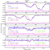 |
Fig. 1. Gaussian fitting of the OH 18 cm lines. From top to bottom are the OH 1665, 1667, 1612, and 1720 MHz lines. Two Gaussian functions fitted to the OH 1667 MHz line are marked with dotted purple and magenta lines. The corresponding counterparts of these two Gaussian components in other lines in the LTE condition are also marked with dotted purple and magenta lines. The conjugate OH satellite lines (absorption in the 1612 MHz line and emission in the 1720 MHz line) are marked with green and orange. The vertical dashed gray line marks the optical redshift. In all subplots, violet lines represent residuals that have been shifted in the Y axis for clarity; the redshifts and their associated uncertainties of individual components are denoted with μ and σ. |
Derived parameters for the OH 18 cm lines.
In the fitting, a crucial assumption is the existence of conjugate OH satellite lines. To test this, we subtracted the thermal absorption counterparts from the OH satellite lines. The remaining and summed spectra are presented in Fig. 2. Both Kolmogorov-Smirnov and Anderson-Darling tests have shown that the summed spectrum is consistent with being drawn from a Gaussian distribution with p values of 0.64 and 0.46, which is strongly suggestive of a conjugate nature. We note that the feature in the residuals at 912.4 MHz has ∼3.7σ significance, which is consistent with a noise peak.
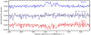 |
Fig. 2. Conjugate OH satellite lines and their summed line. The top and bottom are OH satellite lines with the thermal counterparts subtracted, which have been shifted for clarity, while the middle is the summed spectrum. Both Kolmogorov-Smirnov and Anderson-Darling tests have shown that the summed spectrum is consistent with being drawn from a Gaussian distribution, which strongly suggests that the OH satellite lines are conjugate. |
4. Measuring the cosmological evolution of fundamental constants
We measure the cosmological evolution of the fundamental constants α, μ, and gp using the measured redshifts of the OH 18 cm lines and the equations (Eq. (12) and (13)) given in Chengalur & Kanekar (2003). We note that the electron-proton mass ratio was used in Chengalur & Kanekar (2003) whereas the proton-electron mass ratio was used in later works, such as Bagdonaite et al. (2013) and Kanekar et al. (2018). In this paper, we also define μ as the proton-electron mass ratio.
From the line fitting, we know that there are four OH gas clouds, of which two are thermalized while another two exhibit conjugate behavior. There are named G1, G2, G3, and G4 and their parameters are listed in Table 1. With the Eqs. (12) and (13) in Chengalur & Kanekar (2003), comparisons of the redshifts between ν1667+ν1665 and ν1667–ν1665, and between ν1667+ν1665 and ν1720–ν1612 for G1 give
 (1)
(1)
For G2 we obtain
 (2)
(2)
For G3, a comparison of the redshifts between ν1720+ν1612 and ν1720–ν1612 gives
 (3)
(3)
and for G4, we have
 (4)
(4)
Combining Eq. (1)a and (2)a, weighted based on their uncertainties, and combining Eqs. (1)b, (2)b, (3), and 4, weighted based on their uncertainties, give
 (5)
(5)
A comparison of various CH3OH transitions in this absorber has given Δμ/μ=(−1.8±1.2)×10−7 (Muller et al. 2021). Applying this to Eq. (5) gives
5. Discussion
While measuring the fractional change in fundamental constants has been attempted with spectral lines from different species (e.g., Carilli et al. 2000; Kanekar 2011; Kanekar et al. 2012), velocity offsets between different species introduce redshift differences, which mimic a change in the fundamental constants. Using the lines from the same gas, such as the conjugate OH satellite lines (Darling 2004; Bagdonaite et al. 2013; Kanekar et al. 2018), avoids this systematic uncertainty. One example is in the z = 0.8858 absorption system toward PKS 1830–211, where different transitions of the methanol molecule have provided Δμ/μ=(−1.8±1.2)×10−7 (Muller et al. 2021). Here we use only the OH 18 cm lines from thermalized gas and the conjugate OH 18 cm satellite lines.
Other potential sources of error could arise from the change in the continuum morphology of the background quasar (e.g., Garrett et al. 1997; Lovell et al. 1998; Martí-Vidal et al. 2013) and variability in the absorption spectrum in the millimeter and sub-millimeter bands (e.g., Muller & Guélin 2008; Muller et al. 2014, 2023). From 24 years of observations by various telescopes (Chengalur et al. 1999; Koopmans & de Bruyn 2005; Allison et al. 2017; Gupta et al. 2021), this variability does not appear to affect the centimeter band spectra; this result was also seen between the two MeerKAT observing runs (Gupta et al. 2021; Combes et al. 2021). We therefore do not expect significant errors due to flux or spectral variability.
Compared to the constraint on μ, the constraints on the evolution of  , α, and gp have a low precision. This is because the uncertainties are dominated by the ν1720−ν1612 and ν1667−ν1665 terms, which have redshift uncertainties one and three orders of magnitude higher, respectively, than ν1667+ν1665 (Kanekar & Chengalur 2004). Using other lines, such as the OH main lines at other frequencies (Kanekar & Chengalur 2004), could increase the precision. However, there is as yet no detection of other OH lines toward PKS 1830–211. The H I absorption line was simultaneously detected with the OH 18 cm lines (Combes et al. 2021). However, fitting the H I line requires too many Gaussian functions, which makes it difficult to determine whether they truly represent individual components. Therefore, we excluded the H I line in our analysis. Other molecular absorption lines were detected at frequencies much higher than OH 18 cm lines and show different profiles from OH 18 cm lines (e.g., Bottinelli et al. 2009; Muller et al. 2014, 2024), due to the frequency-dependent radio structure of PKS 1830-211. Therefore, a comparison between OH 18 cm lines and other molecular lines is not appropriate.
To date, measurements of the cosmological evolution of gp remain scarce. Chengalur & Kanekar (2003) reported the first simultaneous constraints on the variation of all the three fundamental constants by comparing line redshifts from different species, with uncertainties on the order of ∼10−3. Since then, to our knowledge, no additional measurements of gp have been reported. In this work, we provide another simultaneous measurement of the cosmological evolution of all three fundamental constants based, however, on the same species.
6. Summary
By utilizing the OH 18 cm absorption lines toward PKS 1830–211 and combining these with previous measurements of the electron-proton mass ratio (Muller et al. 2021), we have obtained (1σ) limits of

over a look-back time of 7.3 Gyr.
Acknowledgments
The authors thank the anonymous referee for the comments that improve this paper. The MeerKAT telescope is operated by the South African Radio Astronomy Observatory, which is a facility of the National Research Foundation, an agency of the Department of Science and Innovation. RSU acknowledges the support from National Science Foundation of China (grant 11988101) and the China Postdoctoral Science Foundation (Grant No. 2024M752979). DL is a New Cornerstone Investigator and is supported by the National Science Foundation of China (grant 11988101). MFG is supported by the National Science Foundation of China (grant 12473019), the China Manned Space Project with No. CMSCSST-2021-A06, the National SKA Program of China (Grant No. 2022SKA0120102), and the Shanghai Pilot Program for Basic Research-Chinese Academy of Science, Shanghai Branch (JCYJ-SHFY-2021-013).
In the local thermodynamic equilibrium, the relative strengths of OH 18 cm lines are 1612:1665:1667:1720 MHz = 1:5:9:1 and, where the pumping is dominated by the intraladder 119 μm transition, the OH 18 cm satellite lines will appear as stimulated absorption (1612 MHz) and emission (1720 MHz) with the same strength, showing conjugate behavior (e.g., Darling 2004; Kanekar et al. 2018; Combes et al. 2021). Under the latter condition, the OH 18 cm main lines are suppressed, exhibiting no absorption or emission.
References
- Allison, J. R., Moss, V. A., Macquart, J. P., et al. 2017, MNRAS, 465, 4450 [Google Scholar]
- Avelino, P. P., Martins, C. J. A. P., Nunes, N. J., & Olive, K. A. 2006, Phys. Rev. D, 74, 083508 [Google Scholar]
- Bagdonaite, J., Jansen, P., Henkel, C., et al. 2013, Science, 339, 46 [NASA ADS] [CrossRef] [Google Scholar]
- Bottinelli, S., Hughes, A. M., van Dishoeck, E. F., et al. 2009, ApJ, 690, L130 [CrossRef] [Google Scholar]
- Carilli, C. L., Menten, K. M., Stocke, J. T., et al. 2000, Phys. Rev. Lett., 85, 5511 [Google Scholar]
- Chandola, Y., Saikia, D. J., Ma, Y. -Z., et al. 2024, ApJ, 973, 48 [Google Scholar]
- Chengalur, J. N., & Kanekar, N. 2003, Phys. Rev. Lett., 91, 241302 [Google Scholar]
- Chengalur, J. N., de Bruyn, A. G., & Narasimha, D. 1999, A&A, 343, L79 [NASA ADS] [Google Scholar]
- Combes, F., Gupta, N., Muller, S., et al. 2021, A&A, 648, A116 [NASA ADS] [CrossRef] [EDP Sciences] [Google Scholar]
- Curran, S. J. 2021, MNRAS, 508, 1165 [Google Scholar]
- Curran, S. J., Kanekar, N., & Darling, J. K. 2004, New Astron. Rev., 48, 1095 [Google Scholar]
- Curran, S. J., Darling, J., Bolatto, A. D., et al. 2007, MNRAS, 382, L11 [Google Scholar]
- Curran, S. J., Tanna, A., Koch, F. E., et al. 2011, A&A, 533, A55 [NASA ADS] [CrossRef] [EDP Sciences] [Google Scholar]
- Damour, T., & Dyson, F. 1996, Nucl. Phys. B, 480, 37 [Google Scholar]
- Damour, T., & Polyakov, A. M. 1994, Nucl. Phys. B, 423, 532 [Google Scholar]
- Darling, J. 2003, Phys. Rev. Lett., 91, 011301 [Google Scholar]
- Darling, J. 2004, ApJ, 612, 58 [Google Scholar]
- Ellingsen, S. P., Voronkov, M. A., Breen, S. L., & Lovell, J. E. J. 2012, ApJ, 747, L7 [Google Scholar]
- Flambaum, V. V., & Kozlov, M. G. 2007, Phys. Rev. Lett., 98, 240801 [Google Scholar]
- Garrett, M. A., Nair, S., Porcas, R. W., & Patnaik, A. R. 1997, Vistas Astron., 41, 281 [Google Scholar]
- Griest, K., Whitmore, J. B., Wolfe, A. M., et al. 2010, ApJ, 708, 158 [Google Scholar]
- Gupta, N., Srianand, R., Baan, W., et al. 2016, in MeerKAT Science: On the Pathway to the SKA, 14 [Google Scholar]
- Gupta, N., Momjian, E., Srianand, R., et al. 2018, ApJ, 860, L22 [Google Scholar]
- Gupta, N., Jagannathan, P., Srianand, R., et al. 2021, ApJ, 907, 11 [Google Scholar]
- Kanekar, N. 2011, ApJ, 728, L12 [Google Scholar]
- Kanekar, N., & Chengalur, J. N. 2004, MNRAS, 350, L17 [Google Scholar]
- Kanekar, N., Langston, G. I., Stocke, J. T., Carilli, C. L., & Menten, K. M. 2012, ApJ, 746, L16 [Google Scholar]
- Kanekar, N., Ubachs, W., Menten, K. M., et al. 2015, MNRAS, 448, L104 [Google Scholar]
- Kanekar, N., Ghosh, T., & Chengalur, J. N. 2018, Phys. Rev. Lett., 120, 061302 [Google Scholar]
- Koopmans, L. V. E., & de Bruyn, A. G. 2005, MNRAS, 360, L6 [Google Scholar]
- Li, L. -X., & Gott, J. R. I. 1998, Phys. Rev. D, 58, 103513 [Google Scholar]
- Lovell, J. E. J., Jauncey, D. L., Reynolds, J. E., et al. 1998, ApJ, 508, L51 [Google Scholar]
- Marciano, W. J. 1984, Phys. Rev. Lett., 52, 489 [Google Scholar]
- Martí-Vidal, I., Muller, S., Combes, F., et al. 2013, A&A, 558, A123 [NASA ADS] [CrossRef] [EDP Sciences] [Google Scholar]
- Muller, S., & Guélin, M. 2008, A&A, 491, 739 [NASA ADS] [CrossRef] [EDP Sciences] [Google Scholar]
- Muller, S., Beelen, A., Guélin, M., et al. 2011, A&A, 535, A103 [NASA ADS] [CrossRef] [EDP Sciences] [Google Scholar]
- Muller, S., Combes, F., Guélin, M., et al. 2014, A&A, 566, A112 [NASA ADS] [CrossRef] [EDP Sciences] [Google Scholar]
- Muller, S., Roueff, E., Black, J. H., et al. 2020, A&A, 637, A7 [EDP Sciences] [Google Scholar]
- Muller, S., Ubachs, W., Menten, K. M., Henkel, C., & Kanekar, N. 2021, A&A, 652, A5 [NASA ADS] [CrossRef] [EDP Sciences] [Google Scholar]
- Muller, S., Martí-Vidal, I., Combes, F., et al. 2023, A&A, 674, A101 [NASA ADS] [CrossRef] [EDP Sciences] [Google Scholar]
- Muller, S., Le Gal, R., Roueff, E., et al. 2024, A&A, 683, A62 [NASA ADS] [CrossRef] [EDP Sciences] [Google Scholar]
- Murphy, M. T., Webb, J. K., & Flambaum, V. V. 2003a, MNRAS, 345, 609 [Google Scholar]
- Murphy, M. T., Webb, J. K., Flambaum, V. V., & Curran, S. J. 2003b, Ap&SS, 283, 577 [Google Scholar]
- Murphy, M. T., Flambaum, V. V., Webb, J. K., et al. 2004, Lecture Notes Phys., 648, 131 [Google Scholar]
- Murphy, M. T., Webb, J. K., & Flambaum, V. V. 2008a, MNRAS, 384, 1053 [CrossRef] [Google Scholar]
- Murphy, M. T., Flambaum, V. V., Muller, S., & Henkel, C. 2008b, Science, 320, 1611 [Google Scholar]
- Nunes, N. J., Dent, T., Martins, C. J. A. P., & Robbers, G. 2009, Mem. Soc. Astron. It., 80, 785 [Google Scholar]
- Rosenband, T., Hume, D. B., Schmidt, P. O., et al. 2008, Science, 319, 1808 [NASA ADS] [CrossRef] [Google Scholar]
- Sandvik, H. B., Barrow, J. D., & Magueijo, J. 2002, Phys. Rev. Lett., 88, 031302 [Google Scholar]
- Schulz, A., Henkel, C., Menten, K. M., et al. 2015, A&A, 574, A108 [NASA ADS] [CrossRef] [EDP Sciences] [Google Scholar]
- Srianand, R., Chand, H., Petitjean, P., & Aracil, B. 2004, Phys. Rev. Lett., 92, 121302 [Google Scholar]
- Su, R., An, T., Curran, S. J., et al. 2025, ApJ, 981, L25 [Google Scholar]
- Tercero, B., Cernicharo, J., Cuadrado, S., de Vicente, P., & Guélin, M. 2020, A&A, 636, L7 [NASA ADS] [CrossRef] [EDP Sciences] [Google Scholar]
- Thompson, R. I. 2013, MNRAS, 431, 2576 [Google Scholar]
- Thompson, R. I., Martins, C. J. A. P., & Vielzeuf, P. E. 2013, MNRAS, 428, 2232 [Google Scholar]
- Tzanavaris, P., Webb, J. K., Murphy, M. T., Flambaum, V. V., & Curran, S. J. 2005, Phys. Rev. Lett., 95, 041301 [Google Scholar]
- Tzanavaris, P., Murphy, M. T., Webb, J. K., Flambaum, V. V., & Curran, S. J. 2007, MNRAS, 374, 634 [Google Scholar]
- Uzan, J. -P. 2003, Rev. Mod. Phys., 75, 403 [Google Scholar]
- Uzan, J. -P. 2011, Liv. Rev. Relativ., 14, 2 [Google Scholar]
- Uzan, J. P. 2024, ArXiv e-prints [arXiv:2410.07281] [Google Scholar]
- Wiklind, T., & Combes, F. 1996, Nature, 379, 139 [Google Scholar]
- Zheng, Z., Li, D., Sadler, E. M., Allison, J. R., & Tang, N. 2020, MNRAS, 499, 3085 [NASA ADS] [CrossRef] [Google Scholar]
All Tables
All Figures
|
Fig. 1. Gaussian fitting of the OH 18 cm lines. From top to bottom are the OH 1665, 1667, 1612, and 1720 MHz lines. Two Gaussian functions fitted to the OH 1667 MHz line are marked with dotted purple and magenta lines. The corresponding counterparts of these two Gaussian components in other lines in the LTE condition are also marked with dotted purple and magenta lines. The conjugate OH satellite lines (absorption in the 1612 MHz line and emission in the 1720 MHz line) are marked with green and orange. The vertical dashed gray line marks the optical redshift. In all subplots, violet lines represent residuals that have been shifted in the Y axis for clarity; the redshifts and their associated uncertainties of individual components are denoted with μ and σ. |
| In the text | |
|
Fig. 2. Conjugate OH satellite lines and their summed line. The top and bottom are OH satellite lines with the thermal counterparts subtracted, which have been shifted for clarity, while the middle is the summed spectrum. Both Kolmogorov-Smirnov and Anderson-Darling tests have shown that the summed spectrum is consistent with being drawn from a Gaussian distribution, which strongly suggests that the OH satellite lines are conjugate. |
| In the text | |
Current usage metrics show cumulative count of Article Views (full-text article views including HTML views, PDF and ePub downloads, according to the available data) and Abstracts Views on Vision4Press platform.
Data correspond to usage on the plateform after 2015. The current usage metrics is available 48-96 hours after online publication and is updated daily on week days.
Initial download of the metrics may take a while.