| Issue |
A&A
Volume 652, August 2021
|
|
|---|---|---|
| Article Number | A30 | |
| Number of page(s) | 20 | |
| Section | Extragalactic astronomy | |
| DOI | https://doi.org/10.1051/0004-6361/202039738 | |
| Published online | 04 August 2021 | |
The emergence of passive galaxies in the early Universe
1
INAF – Osservatorio Astronomico di Roma, Via di Frascati 33, 00078 Monte Porzio Catone, Italy
e-mail: This email address is being protected from spambots. You need JavaScript enabled to view it.
2
Department of Physics and Astronomy and PITT PACC, University of Pittsburgh, Pittsburgh, PA 15260, USA
3
Argelander-Institut für Astronomie, Universität Bonn, Auf dem Hügel 71, 53121 Bonn, Germany
4
Centre for Astrophysics Research, School of Physics, Astronomy & Mathematics, University of Hertfordshire, Hatfield AL10 9AB, UK
5
Astronomy Centre, Department of Physics and Astronomy, University of Sussex, Brighton BN1 9QH, UK
Received:
21
October
2020
Accepted:
10
May
2021
Abstract
The emergence of passive galaxies in the early Universe results from the delicate interplay among the different physical processes responsible for their rapid assembly and the abrupt shut-down of their star formation activity. Investigating the individual properties and demographics of early passive galaxies improves our understanding of these mechanisms. In this work we present a follow-up analysis of the z > 3 passive galaxy candidates selected by Merlin et al. (2019, MNRAS, 490, 3309) in the CANDELS fields. We begin by first confirming the accuracy of their passive classification by exploiting their sub-millimetre emission to demonstrate the lack of ongoing star formation. Using archival ALMA observations we are able to confirm at least 61% of the observed candidates as passive. While the remainder lack sufficiently deep data for confirmation, we are able to validate the entire sample in a statistical sense. We then estimate the stellar mass function (SMF) of all 101 passive candidates in three redshift bins from z = 5 to z = 3. We adopt a stepwise approach that has the advantage of taking into account photometric errors, mass and selection completeness issues, as well as the Eddington bias, without any a posteriori correction. We observe a pronounced evolution in the SMF around z ∼ 4, indicating that we are witnessing the emergence of the passive population at this epoch. Massive (M > 1011 M⊙) passive galaxies, only accounting for a small (< 10%) fraction of galaxies at z > 4, become dominant at later epochs. Thanks to a combination of photometric quality, sample selection, and methodology, we overall find a higher density of passive galaxies than in previous works. The comparison with theoretical predictions, despite a qualitative agreement (at least for some of the models considered), denotes a still incomplete understanding of the physical processes responsible for the formation of these galaxies. Finally, we extrapolate our results to predict the number of early passive galaxies expected in surveys carried out with future facilities.
Key words: galaxies: evolution / galaxies: high-redshift / galaxies: luminosity function, mass function / methods: data analysis
© ESO 2021
1. Introduction
In the last 10−15 years, it has become evident that massive passive galaxies were already in place at earlier and earlier epochs (e.g. Cimatti et al. 2004; Saracco et al. 2005; Labbé et al. 2005; Kriek et al. 2006; Grazian et al. 2007; Fontana et al. 2009; Straatman et al. 2014; Nayyeri et al. 2014; Schreiber et al. 2018a; Merlin et al. 2018, 2019; Carnall et al. 2020; Shahidi et al. 2020). The very existence of massive galaxies with suppressed star formation at z > 3 poses a serious challenge to theoretical predictions, which struggle to reproduce sufficiently intense star formation rates (SFRs) at even higher redshift to assemble such large stellar masses (> 1010 − 1011 M⊙) and prevent further gas collapse at least until the epoch of observation (Fontana et al. 2009; Vogelsberger et al. 2014; Feldmann et al. 2016; Merlin et al. 2019; Shahidi et al. 2020). Despite the difficulties associated with their search, substantially owing to their faintness in the UV rest frame commonly used to select high-redshift galaxies and their spectroscopic confirmation, studying and deeply understanding these systems helps us shed light on their rapid formation process and similarly rapid quenching mechanism.
This paper is the fourth in a series. In our first work (Merlin et al. 2018) we presented an accurate and conservative technique to single out passive galaxies at high redshift by means of spectral energy distribution (SED) fitting with a probabilistic approach. We selected 30 z > 3 candidates in the GOODS-S field. Passive galaxy candidates, while being relatively easy to select from photometric surveys once the technique is established, need to be confirmed by other means. This is usually achieved through spectroscopic observations. However, spectroscopy becomes particularly difficult and time consuming at z > 3, where only few candidates have been confirmed so far (Glazebrook et al. 2017; Schreiber et al. 2018a; Tanaka et al. 2019; Valentino et al. 2020; Forrest et al. 2020a,b; Saracco et al. 2020; D’Eugenio et al. 2020). In our second work (Santini et al. 2019, S19 hereafter), we used a complementary approach and looked for evidence of the lack of star formation as seen in the sub-millimetre regime to confirm the passive classification of the high-z candidates selected in GOODS-S. At that time, we could confirm 35% of the targets on an individual basis adopting conservative assumptions, and we validated the sample as a whole in a statistical sense. In our third work (Merlin et al. 2019, M19 hereafter), we extended the search for passive galaxies to the entire CANDELS sample and selected 102 z > 3 candidates over the five fields. In the present work, we first confirm the passive nature of these candidates, adopting the method presented in S19 and taking advantage of the richer ALMA archive, which includes observations that were still proprietary at the time of our previous work. We then analyse the emergence and mass growth of this peculiar class of galaxies by means of two powerful statistical tools: the stellar mass function (SMF) and the stellar mass density (SMD). Very few studies so far have pushed the analysis of the SMF of passive galaxies at z > 3 (Muzzin et al. 2013; Davidzon et al. 2017; Ichikawa & Matsuoka 2017; Girelli et al. 2019) because of the difficulty in assembling statistically meaningful samples of candidates at such high redshift.
The paper is organized as follows. We present the data set and recall how passive galaxies are selected in Sect. 2; in Sect. 3 we confirm the passive nature of the sample by means of ALMA public observations; Sect. 4 illustrates the method adopted to compute the SMF; our results are presented in Sect. 5 and compared with previous observations and theoretical predictions in Sect. 6; based on our SMF, in Sect. 7 we predict the number of high-z passive galaxies expected from future facilities; finally, we summarize the main findings of this work in Sect. 8. In the following, we adopt the Λ cold dark matter (CDM) concordance cosmological model (H0 = 70 km s−1 Mpc−1, ΩM = 0.3, and ΩΛ = 0.7) and a Salpeter (1955) initial mass function (IMF). All magnitudes are in the AB system.
2. Data set and sample selection
We briefly summarize the major characteristics of the CANDELS data set and the strategy adopted to select passive galaxies; the relevant publications are noted for further details.
The Cosmic Assembly Near-infrared Deep Extragalactic Legacy Survey (CANDELS; Koekemoer et al. 2011; Grogin et al. 2011; PIs: S. Faber and H. Ferguson) is the largest (902 orbits) HST programme ever approved, and it has observed the distant Universe with the WFC3 and ACS cameras. It has targeted five fields, covering a total area of ∼1000 sq. arcmin. The multiwavelength photometric catalogues have been publicly released and are fully described in the relevant accompanying papers (Guo et al. 2013 for GOODS-S, Barro et al. 2019 for GOODS-N, Galametz et al. 2013 for UDS, Stefanon et al. 2017 for EGS and Nayyeri et al. 2017 for COSMOS). For GOODS-S we used an improved catalogue including three more bands (WFC3 F140W, VIMOS B, and Hawki-Ks from the HUGS survey; Fontana et al. 2014) and improved photometry on the Spitzer bands thanks to new mosaics (IRAC CH1 and CH2, by R. McLure) and new software (all four channels were re-processed using T-PHOT; Merlin et al. 2015). These improvements are discussed in Merlin et al. (2021). For the remaining fields we used the official catalogues.
We adopted the photometric redshifts from the latest CANDELS estimates (Kodra 2019), and these will be presented in Kodra et al. (in prep.). These improve upon the original released photometric redshifts presented in Dahlen et al. (2013) and are based on a combination of four independent photo-z probability distribution functions (unless spectroscopic redshifts are available), using the minimum Frechet distance combination method.
2.1. Selection of high-z passive candidates
The present work is based on the z > 3 passive galaxy sample selected by M19 in the five CANDELS fields. Candidates were identified by means of an ad hoc developed SED fitting technique that is fully described in Merlin et al. (2018). Briefly, we used Bruzual & Charlot (2003) stellar population models and assumed ‘top-hat’ star formation histories (SFH); these are characterized by a period of constant star formation followed by an abrupt truncation of the star formation that is set to zero thereafter. Despite being over-simplified, these analytic shapes manage to mimic the rapid timescales available for quenching at high redshift; these timescales are comparable to the age of the Universe and they are at variance with those required by standard exponential models, which reach quiescence in not less than ≲1 Gyr. Moreover, the adoption of top-hat SFHs is an improvement over a standard UVJ selection since the fit is able to identify recently quenched sources, still showing blue U − V colours.
In addition to being fit in their passive phase (i.e. with zero SFR), candidates also need to pass conservative selection criteria based on the probability P(χ2) of the χ2 resulting from the fitted solution. In the end, to be classified as passive, galaxies need to fulfil the following criteria: (a) H < 27; (b) 1σ detection in K, IR1 and IR2 bands; (c) zphot > 3; (d) SFRbest = 0; and (e) P( ) > 30% and P(
 ) < 5%. The last requirement ensures that the best-fit passive solution has a high probability P(
 ) and at the same time that no plausible (i.e. with P(
 ) > 5%) star-forming solutions exist.
We ended up with a sample of 102 galaxies (the so-called reference sample in M19; i.e. that obtained without inclusion of emission lines in the fit). Candidates are distributed quite inhomogeneously across the fields: 33 in GOODS-S, 36 in GOODS-N, 16 in UDS, 13 in EGS, and 4 in COSMOS. The variance across the fields cannot be entirely explained by cosmic variance, but probably reflects the different photometric properties of the five catalogues. In particular, they differ in the depth of the K and IRAC bands (see M19). All candidates have redshift lower than 5 except one source in GOODS-N (zphot ∼ 6.7; discussed in M19). In the following, we restrict ourselves to the 3 < z < 5 sample, made of 101 galaxies. The final list of passive candidates is presented in Tables A.1–A.5.
Among our passive galaxies, four are flagged as X-ray detected active galactic nuclei (AGNs) in GOODS-S (one of which is a confirmed AGN; see M19), three in GOODS-N, and two in EGS. Two of the AGN candidates in GOODS-S are also detected by Herschel (see Santini et al. 2019); this is likely as result of the emission of the host dust heated by the central nucleus. We believe the AGN candidates are therefore obscured, or at least not bright, Type 1 AGNs. The AGN emission does not significantly affect the estimate of the stellar mass for obscured AGNs, as demonstrated by Santini et al. (2012). For this reason, we did not exclude AGNs from the sample.
Figure 1 shows the redshift distribution of our passive candidates, colour-coded according to the field they belong to. The majority of these candidates are below redshift 4, but the distribution shows a non-negligible tail to higher redshift (12 galaxies at 4 < z < 5).
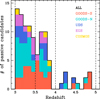 |
Fig. 1. Redshift distribution of the 3 ≤ z < 5 passive candidates used in the present analysis. Different colours show the counts in the various fields (see legend). The open black histogram shows the total sample. |
2.2. Stellar masses
Stellar masses were estimated by SED fitting the observed near-UV to near-IR photometry up to 5.5 μm rest frame to libraries built on Bruzual & Charlot (2003) stellar population synthesis models. For passive galaxies stellar masses were obtained from the fit with top-hat SFHs without including emission lines, as discussed in Sect. 2.1. The grid in stellar ages, burst duration, metallicities, and dust extinction is detailed in M19 (see their Appendix A). The mass distribution of passive candidates in the redshift intervals used in the present analysis is shown in Fig. 2.
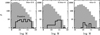 |
Fig. 2. Mass distribution of the passive galaxies (open black histograms) compared to the overall galaxy population (shaded grey histograms) in different redshift bins. |
To test the reliability of the inferred stellar masses we explored the possibility that our candidates host an ongoing dusty burst, misinterpreted as an old stellar population in our fits. We therefore built a stellar library by combining an old, unobscured or moderately obscured burst finished by at least 100 Myr with a star formation episode ongoing since 50 Myr. We fit our GOODS-S candidates with this two-component library and found very similar stellar masses, with a median Mtophat/M2comp of 0.96 and semi-interquartile range of 0.12. We also found that in 29 out of 33 candidates the fit prefers solutions with purely old stellar populations and that in the remaining 4 sources the young stellar population contributes by no more than 20% in mass. This very same result is found by fitting mock galaxies that are purely passive, indicating that in a small fraction of objects (13%) the fit is limited by parameter degeneracy.
For the whole galaxy population we adopted exponentially declining models (τ-models) to parameterize the SFH. The library was built following previous works (e.g. Fontana et al. 2004; Santini et al. 2009; Grazian et al. 2015): metallicities range from Z = 0.02 Z⊙ to Z = 2.5 Z⊙; 0 < E(B − V) < 1.1 with a Calzetti et al. (2000) or Small Magellanic Cloud (Prevot et al. 1984) extinction curve, left as a free parameter; the timescale for the exponentially declining SFH ranges from 0.1 to 15 Gyr; the age (defined as the time elapsed since the onset of star formation) varies within a fine grid and, at a given redshift, is set lower than the age of the Universe at that redshift. The mass distribution of the whole population is shown in Fig. 2.
While very effective in selecting quiescent galaxies at high redshift, the adoption of top-hat models does not have a strong impact on stellar masses. This confirms the results of Santini et al. (2015), who found that the stellar masses are stable against the choice of the SFH parameterization and differences in the metallicity, extinction, and age parameter grid sampling. However, as we discussed in our previous work, while the stellar mass is on average a relatively stable parameter, it can vary for some peculiar sub-classes of objects for which a different SFH parameterization is necessary, such as passive galaxies at high redshift.
Figure 3 shows a comparison between stellar masses obtained with τ-models and with top-hat models, for the whole population in the redshift range of interest and for the passive candidates. Despite being slightly skewed towards larger Mτ/Mtophat ratios (⟨log Mτ/Mtophat⟩ = 0.06 and 0.09 for the passive and global population, respectively), the distributions are peaked at unity, and the mean value is well within the standard deviation of the distribution (0.10 and 0.16, respectively). This mean value is also smaller than the average error bar associated with the estimate of the stellar mass (∼0.4 dex for the entire M > 109 M⊙ sample, ∼0.2 dex at M > 1010 M⊙). We conclude that the two stellar mass estimates agree well for the large majority of sources. A systematics however appears for the passive candidates, whose distribution of log Mτ/Mtophat shows a secondary peak at ∼0.2 dex. This feature is entirely due to candidates with stellar mass below 1010.5 M⊙, which show a broad (or slightly bimodal) distribution between 0 and 0.2 dex. The objects showing the largest mismatch (≳0.1 dex) were fitted with implausibly low values for the stellar metallicity (0.02 times solar) in the τ-model library, which was built for the global galaxy population and not optimized for passive sources. For this reason, in the following, when computing the SMF for the entire galaxy population, we replaced the stellar mass values of the passive candidates with the results obtained from the top-hat library, which we consider more appropriate for this class of objects.
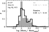 |
Fig. 3. Distribution of the ratio of the stellar mass computed with τ-models to those with top-hat SFHs. The shaded grey histogram refers to the total population of H < 27 galaxies at 3 ≤ z < 5 with Mτ > 109.5 M⊙ in the five CANDELS fields, while the open black histogram shows the passive candidates. The numbers in the upper right corner show the mean and standard deviation of the two distributions. |
3. Confirmation of the passive nature of the candidates from their sub-millimetre emission
One powerful possibility to validate the passive classification of photometrically selected candidates is to measure their far-infrared (FIR) and/or sub-millimetre emission used to exclude ongoing star formation. This method allows us to avoid possible degeneracies between dusty star-forming and old passive solutions in the optical fit. In M19 we cross-matched our sample with Herschel catalogues. For the GOODS fields we took advantage of the new, deep ASTRODEEP catalogues by Wang et al. (in prep.), which combine data from PEP (Lutz et al. 2011) and GOODS-Herschel (Elbaz et al. 2011) surveys for the PACS bands and from the HerMES survey (Oliver et al. 2012) for the SPIRE bands. For COSMOS and EGS we used PEP-PACS and HerMES-SPIRE catalogues (Roseboom et al. 2010, 2012). For the UDS field we used HerMES catalogues for both cameras. As discussed in our previous work, with the exception of two sources in GOODS-S (GOODSS-10578 and GOODSS-3973), which are likely obscured AGNs (see discussion in Merlin et al. 2018, S19, M19 and in Sect. 3.2.1), no clear evidence for FIR emission was found. This test is however limited by poor sensitivity at these redshifts and a high level of confusion. For this reason, we attempted to extract more information out of Herschel maps by stacking. We stacked all sources at 100 and 160 μm, offering the best compromise between depth and angular resolution among all Herschel bands. We did not measure any flux above the noise level in any of the five fields individually nor in the combination of these fields. We note, however, that the depth of stacked Herschel maps, resulting into a typical limiting SFR of ∼100 (600) M⊙ yr−1 from 100 μm (160 μm), is not sufficient to reject mild levels of SFR in these galaxies. For this reason we opted for ALMA data to confirm the passive solutions of our candidates.
We took advantage of the rich ALMA archive and extended the very same analysis described in S19 to the entire CANDELS sample of high-z passive candidates. In the following, we summarize the main steps and present the new results. Further details are available in S19.
3.1. ALMA archival observations
Out of the five CANDELS fields, only three are accessible by ALMA (GOODS-S, UDS, and COSMOS). This reduces the number of candidates over which the validation method can be attempted to 53. A search in the ALMA archive returned observations in Band 6 and 7 for 41 of the candidates. Nine candidates in UDS and three candidates in COSMOS have been observed in Band 7; one of the COSMOS candidates has also been observed in Band 6. Of the GOODS-S candidates, 21 and 19 candidates have been observed in Band 6 and 7, respectively; 11 have been observed in both bands. Band 3 and 4 observations, available for a fraction of the sources, give less stringent constraints and have not been used.
We produced images with ≥0.6 arcsec spatial resolution using natural weightings and uv tapers when needed. In this way, we could assume that sources are unresolved (see justification and references in S19) and maximize the sensitivity to detection. We note that given the native angular resolution of the data, the maximum recoverable scale is > 1.5 arcsec (0.75 arcsec in a couple of cases). Assuming a homogenous surface brightness, this results in a physical scale of > 10 kpc (∼5 kpc) at the redshifts of our sources. The typical size of z > 2 sources measured by Fujimoto et al. (2017) on ALMA Band 6 and 7 images (Re < 3 kpc, with an avearage value of ∼1 kpc) makes us confident that the emission of our targets is not filtered out by the reduction process.
The sub-millimetre flux was read directly on the map (in units of Jy beam−1) as the value of the pixel at the position of the source. The associated uncertainty was taken as the standard deviation of all pixels with similar coverage, after excluding the position of the candidate and other potential sources in the image (see S19). In order to avoid astrometry issues, if the source is detected at more than 3σ, we replaced the value of the flux at the centre with the maximum value within the beam; if, on the other hand, the source is undetected, we used the mean flux within the beam. We finally stacked sources observed more than once in the same band by averaging the fluxes measured from different programmes and weighting these fluxes with the associated errors; the final sensitivity per beam was inferred as the standard error on the weighted mean.
The achieved median sensitivity is 0.17 mJy in Band 6 and 0.25 mJy in Band 7; there is a semi-interquartile range of scatter among the various sources of ∼0.07 in both cases. Only one of the 41 sources is detected at > 3σ level (GOODSS-3973, S870 μm = 0.74 ± 0.18 mJy). Six sources are barely above the noise level (at 1−2σ level). We report the ALMA flux in the most stringent band in Tables A.1–A.3. No significant detection is found even after stacking all observations in the same band (including the only detected source), either over the entire redshift range or in bins of redshift (3 < z < 4 and 4 < z < 5).
3.2. Method
Sub-millimetre fluxes were converted into estimates of (or in most cases upper limits on) the SFR by fitting these fluxes to a number of IR models. We considered the average SMG SEDs of Michałowski et al. (2010) and Pope et al. (2008), the two average SEDs fitted by Elbaz et al. (2011) for main sequence (MS) and starburst galaxies, and the full libraries of Chary & Elbaz (2001), Dale & Helou (2002), and Schreiber et al. (2018b). The latter library has the dust temperature Td as free parameter, whose choice highly affects the inferred SFR. We considered two templates, one with Td = 25 K, as conservatively expected for quiescent galaxies (Gobat et al. 2018; Magdis et al. 2021) and one with light-weighted Td = 40−50 K, as predicted by the redshift evolution of the dust temperature parameterized by Schreiber et al. (2018b). We assumed RSB = SFR/SFRMS = 1. As done in S19, in the following we adopted the template of Michałowski et al. (2010) as a reference model. We converted the inferred total infrared luminosity between 3 and 1100 μm adopting the calibration of Kennicutt & Evans (2012), adjusted to a Salpeter IMF using their conversion factor. The SFR was calculated at the redshift of the candidates and at any given redshift between 0 and 6. For the majority (10 out of 12) of the candidates observed in Band 6 and 7, we used the former band because the data turned out to be more stringent in terms of the resulting SFR. The median limiting SFR is ∼43 M⊙ yr−1 (∼55 M⊙ yr−1 at z > 4) and has a semi-interquartile range of ∼15 M⊙ yr−1. The inferred SFRs are listed in Tables A.1–A.3. We note that any possible contribution from evolved stellar populations to the FIR luminosity would decrease the inferred SFR, and therefore would make our results even stronger.
As discussed in S19, the spread in the inferred SFR among different templates is not negligible; the spread may span even a decade when fitting to the longest wavelength Band 6 data. As a consequence, the exact value of the SFR is subject to this systematics. However, although we discuss the results based on the reference model of Michałowski et al. (2010), we note that our conclusions are solid against the choice of the IR templates. We used two approaches to validate the passive solutions of the optical fit.
3.2.1. Validation of individual candidates
To make sure that our candidates were not erroneously best fit by passive templates, we checked whether or not the alternative star-forming solutions are compatible with ALMA results. To this aim, we compared the SFR inferred from ALMA data, or in most cases the 3σ limits on the SFR, as a function of redshift to any plausible (i.e. with associated χ2 probability larger than 5%) star-forming solution of the optical fit obtained at any redshift. The fit was re-run with redshift set as a free parameter, instead of fixed to the best-fit photo-z where, by definition, there are no star-forming solutions with probability larger than 5%.
For 61% of the observed candidates (including the only detected source), ALMA constraints predict a SFR that, at any redshift, is below the optical solution, or in most cases no star-forming solutions exist at all. In other words, the very red colours of the candidates cannot be justified by a large amount of dust, but need to be explained by old stellar populations. This implies that the optical star-forming solutions are implausible, therefore supporting the passive best fit. These sources are robustly and individually confirmed as passive at a 3σ confidence level, and the result is unaffected by the choice of the IR template used to calculate the SFR; we note that even more sources would be confirmed by adopting more conservative templates. The last column of Tables A.1–A.3 indicates the candidates that have been individually confirmed. For the rest of the sample, ALMA upper limits are above the optical star-forming solutions, making the comparison inconclusive. Deeper sub-millimetre data would be needed to confirm (or reject) the passive nature of these sources. This comparison is graphically represented in Fig. 3 of S19 for the GOODS-S candidates of Merlin et al. (2018). The improvement in the fraction of validated candidates compared to S19 results is explained by two effects. In part, the adoption of updated redshifts for the search of passive galaxies leads to a more reliable selection. Most importantly, our previous work relies on the exceedingly conservative choice of adopting, for this test, the nebular line fit for all candidates, even for those selected without their inclusion.
Among the candidates that have been individually confirmed as passive are the two GOODS-S candidates, GOODSS-10578 and GOODSS-3973, with associated Herschel (and MIPS) emission; GOODSS-3973 was also detected by ALMA. Although it may at first be surprising, as fully discussed in Merlin et al. (2018), S19, and M19, these two sources are likely obscured AGNs. Both GOODSS-10578 and GOODSS-3973 are identified as X-ray emitters in the Chandra catalogue of Cappelluti et al. (2016) and the former is also confirmed as an AGN by the MUSE deep data (Inami et al. 2017). Their IR emission is likely associated with hot dust heated by the central AGN rather than cold dust heated by UV stars and tracing ongoing star formation. As a matter of fact, the mid-IR emission of these two sources is at least a factor of 10 (if not 100, depending on the chosen model) higher than predicted when fitting the ALMA flux with purely star-forming IR templates (see Sect. 3.2 and S19). Similarly, the recent analysis of D’Eugenio et al. (2020) finds four secure 24 μm detections out of their 10 z ∼ 3 spectroscopically confirmed passive galaxies with no FIR counterparts, three of which are consistent with being AGN-powered. Based on a mean stack radio detection these authors derive similar limiting SFR as individually measured by us from ALMA data. Furthermore, Spitler et al. (2014) find six 24 μm detections among their 26 massive quiescent (based on a UVJ selection) 3 < z < 4 candidates, three of which show signs of AGN. In conclusion, the presence of 24 μm emission in passive candidates is not totally unexpected and is likely associated with AGN activity.
3.2.2. Statistical validation of sample
Since the available ALMA data are not deep enough to draw any conclusions for 39% of the observed candidates, we tried to validate the passive nature of the entire sample in a statistical sense. To this aim, we adopted 1σ limits in the following.
We first repeated the procedure described above on the stacked flux in Band 6 and 7, which is compared to the collection of star-forming solutions of all sources included in the stacks. We found that the sample is on average consistent with being passive; a group of solutions with low SFR values, below the ALMA limits, are observed in Band 7, but this can be ascribed to a minor fraction of sources (i.e. 10% of the stacked sample). Once again the result is robust against the uncertainty in modelling the IR SED. Indeed, the results are only inconclusive when adopting two of the models (Pope et al. 2008; Schreiber et al. 2018b with high dust temperature), but again due to a minority of sources.
We then adopted an independent approach to verify how the SFR of the candidates compares with that of typical star-forming galaxies. We made use of the stellar mass inferred from the optical fit (a much more robust parameter than the SFR, as discussed above; see also Santini et al. 2015) and of the sub-millimetre-based SFRs, and compared the position of the candidates on a SFR-stellar mass diagram with the location of the MS of star-forming galaxies. In Fig. 4 we show all candidates observed by ALMA divided into two redshift bins, compared with the observed (i.e. not corrected for the Eddington bias) MS inferred from HST Frontier Field data by Santini et al. (2017). We found that 59% of the candidates are located below the 1σ scatter of the MS (0.3 dex), while 39% and 27% are at least 2σ and 3σ below of the MS, respectively, that is in the region in which we expect to find sources that have completely exhausted their star formation. The fraction of sources at least 1σ, 2σ, and 3σ below the MS are in the ranges 39−80%, 24−68%, and 2−41%, depending on the choice of the IR template (46−80%, 34−68%, and 5−41%, respectively, if the most extreme template is ignored). In the figure, we highlight the candidates that have been individually and robustly confirmed (Sect. 3.2.1). The majority of these candidates are located below the MS. However, a fraction of the confirmed sources have less stringent constraints, placing these sources around the MS. We note that, with the exception of one source with huge error bars extending down to the passive area of the diagram, the rest of the candidates around the MS only have upper limits on the SFR. Knowledge of their exact position is hampered by the available data and they may in principle have much lower levels of SFR. The fact that some of these candidates are individually confirmed as passive makes us confident that even the sources with shallow sub-millimetre constraints preventing their individual confirmation may be intrinsically passive.
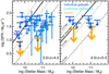 |
Fig. 4. Location of the passive candidates observed by ALMA on a SFR-stellar mass diagram, in two redshift bins, based on their sub-millimetre SFR. The arrows represent 1σ upper limits on the SFR. The 1σ error bars on the stellar masses have been conservatively calculated by setting the redshift as a free parameter. The solid lines show the observed MS of Santini et al. (2017). The dotted lines are 1σ above and below the MS (estimated from the observed 0.3 dex scatter), while the dashed line is 3σ below the MS. Individual sources are shown in blue. Robust candidates (i.e. individually confirmed as passive at a 3σ confidence level) have been overplotted in light blue. The large orange symbols show the stacks in bins of stellar mass, denoted by the vertical dotted orange lines. |
We finally stacked sources in bins of stellar mass (orange symbols in Fig. 4). Once again, the stacking analysis supports the passive classification of the whole sample. The stacked SFR is well below the MS, with the exception of the lowest mass bin in both redshift intervals, where available sub-millimetre data are not deep enough to reach the lower level of the typical SFR of low-mass galaxies. The only IR template unable to confirm the stacking results with high significance is the high dust temperature template of Schreiber et al. (2018b), yielding a high-z/high-M stacked SFR only ∼1.3σ below the MS.
We note that, once the sample is confirmed as passive, either for individual sources or statistically, ALMA fluxes can be fit with the IR passive template of Magdis et al. (2021). This template yields an approximiately five times lower SFR, and places 95%, 78%, and 66% of the candidates 1σ, 2σ, and 3σ below the MS; basically all sources with log M/M⊙ > 10.4 are at least 0.9 dex below the MS according to this template.
3.3. Conclusions
We used ALMA archival observations to confirm the passive nature of our candidates. By means of the (lack of) sub-millimetre emission, we could validate the passive classification for 61% of the candidates observed by ALMA at a 3σ confidence level. At the same time, based on the available data, we could not reject any of the candidates and found that the sample is on average consistent with being correctly classified as passive. This result is solid against the large systematics associated with the choice of the IR template when computing the SFR from sub-millimetre emission. Only one model, that characterized by the highest dust temperature, appears to be unable to statistically confirm the entire sample with high significance, but we note that this is the most extreme template, and the assumed temperature is at the highest envelope of the Td distribution (Faisst et al. 2020; see also the extrapolation to high-z of the results of Magnelli et al. 2014 or Genzel et al. 2015).
Once again we confirmed the reliability and robustness of the photometric selection technique developed in Merlin et al. (2018) and M19. Assuming our technique performs equally well on the sources unobserved by ALMA, in the following we consider the entire sample of 101 3 < z < 5 passive galaxy candidates.
4. Determination of the galaxy stellar mass function
To estimate the SMF, we adopted the stepwise method, which is a non-parametric approach that has the advantage of not assuming an a priori shape for the SMF (e.g. Takeuchi et al. 2000; Bouwens et al. 2008; Weigel et al. 2016). Instead, the stepwise estimate assumes that the SMF can be approximated by a binned distribution, where the number density  in each mass bin j is a free parameter.
In particular, we adopted the procedure presented in Castellano et al. (2010; Sect. 6.2.2). We assumed a fixed, constant, reference density ϕref over the entire mass range and exploited a simulation to compute the distribution of observed stellar masses originating in each mass bin, as a consequence of the percolation of sources across adjacent bins caused by photometric scatter or failure in the selection technique to isolate simulated passive galaxies. To take field-to-field variations in depth and selection effects into account, the simulations were run for each field separately, scaled to the relevant observed areas, and eventually summed to obtain the total number densities predicted in each mass bin. The intrinsic densities are expressed as  , where wj are the multiplicative factors to the reference density of the simulation. The intrinsic densities, hence the multiplicative factors, and relevant uncertainties, which best reproduce the observed number densities
  of our survey, were determined by inverting the linear system
  ), where Sij are the elements of the transfer function computed from the simulation; that is Sij is essentially the number of galaxies in the mass bin i scattered from the bin j and taking the sources missed by the selection into account. The bin size was chosen as a compromise between the need to have reasonable statistics in each bin and the desire to sample the shape of the SMF with good mass resolution.
Simulated masses were obtained by redshifting between z = 3 and z = 5 a subset of the synthetic spectra of the stellar libraries. We chose the library parameters to reproduce the observed mass-to-light ratios in the rest-frame I band of the passive candidates and the entire 3 ≤ z < 5 sample. For the passive sources we only considered passive templates. Each template was then normalized to stellar masses between 9 and 12 in the logarithmic space. The final simulations are made of 32893 templates for the top-hat library and 43044 templates for the τ-models library. The simulations were designed to reproduce the average and the scatter of the observed S/N as a function of magnitude to provide the closest match between observed and simulated data, as done in Castellano et al. (2012). Differences in depth, and therefore selection effects, among the different fields are taken into account by running the simulation independently for each of the fields. In addition, the two GOODS fields have inhomogeneous coverage in the HST bands. While the difference in depth between the CANDELS wide and deep areas is accounted for by the scatter of the error-magnitude relation, this is not true for the ultra-deep GOODS-S area (4.6 arcmin2, Guo et al. 2013). For this reason, we treated the latter as a separate field with its own simulation. For each field, synthetic fluxes were obtained by convolving the synthetic templates with the filter response curves and were perturbed with noise in a way to mimic the field properties in terms of depth. We then fitted these simulated catalogues and selected simulated passive galaxies in the very same way as done on real data. For the total population, we simply selected H < 27 galaxies. We verified that the resulting mass-to-light ratio distribution agrees well with the input distribution; this makes us confident that mass-to-light ratios are not substantially modified by observational errors.
Although the simulation covers stellar masses from 109 to 1012 M⊙, in the following we consider the SMF on a narrower range of masses. The required corrections below 1010 M⊙ make the SMF very uncertain at these low masses. However, low-mass bins need to be included in the procedure to consider the effect of the Malmquist bias, that is to account for low-mass sources scattered to larger measured masses. The overall corrections applied to the observed counts are within a factor of 3; the only exception is the lowest mass bin at z > 3.5, affected by a higher level of incompleteness, where the required correction is a factor of 5 and 10 at intermediate and high redshift, respectively.
The stepwise method has the advantage of taking mass completeness issues, incompleteness in the passive selection, photometric errors (i.e. the percolation of sources across adjacent mass bins), and the Eddington bias into account. The Eddington bias is naturally accounted for without any a posteriori simulation. As shown by Davidzon et al. (2017), stepwise results show very good agreement with the standard 1/Vmax method. As an additional test, we verified that the SMF computed with the stepwise approach on the GOODS-S sample, using the very same photometric catalogue, redshifts, and sample selections as Grazian et al. (2015), nicely agrees with their 1/Vmax points.
The cumulative area over which the SMF was calculated is 969.7 arcmin2. Cosmic variance has been added using the QUICKCV code of Moster et al. (2011). It computes relative cosmic variance errors as a function of stellar mass, in bins very similar to those used in this work, up to 1011.5 M⊙. For the largest mass bin, we adopted the value for the 11−11.5 logarithmic bin incremented by 50%. We verified that this particular choice does not significantly affect our results. Since cosmic variance not only depends on the total area surveyed but also on the survey geometry, following Driver & Robotham (2010), we reduced these relative errors by  , where N = 5 is the number of non-contiguous fields of similar area.
Finally, Schechter functions were fitted to the stepwise points and uncertainties. As discussed in Sect. 2.1, we did not exclude AGN candidates from the sample. In any case, we verified that the exclusion of the nine X-ray detected candidates among the passive sample (and similar exclusion from the total sample) does not change our results.
5. The SMF and stellar mass density of 3 ≤ z < 5 passive galaxies
The resulting SMF for the passive population, computed in three different redshift bins, is shown in Fig. 5 and reported in Table 1. We also show the best-fit Schechter functions and the associated 68% probability confidence regions. As a consequence of the lack of constraints at low masses and larger uncertainties at high redshift, at z > 3.5 we fixed the value of the slope α to its best-fit value in the lowest redshift bin. The best-fit Schechter parameters are listed in Table 2.
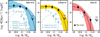 |
Fig. 5. SMF for passive galaxies in the five CANDELS fields. The solid black points show the stepwise results; the error bars account for Poissonian and cosmic variance uncertainties. The black curves show the Schechter fits and the coloured shaded areas indicate the regions at 68% confidence level considering the joint probability distribution function of the Schechter parameters. The open blue symbols and lines show the SMF for passive galaxies taken from the literature, scaled to a Salpeter IMF, in the same (or very similar) redshift bins (Ichikawa & Matsuoka 2017 as squares, Davidzon et al. 2017 as a dashed line, and McLeod et al. 2021 as a dot dashed line), and at slightly different redshifts (Muzzin et al. 2013 as triangles and Girelli et al. 2019 as 6-point stars). |
Stellar mass function of passive galaxies as inferred from a stepwise method.
Best-fit parameters and their 1σ uncertainties in the different redshift intervals derived from fitting the stepwise SMF with a Schechter function.
A strong evolution in the ‘knee’ of the SMF (M*) is observed around z ∼ 4. For a better visualization of the evolution in the SMF, in Fig. 6 we show the three redshift bins simultaneously. Despite the large associated uncertainties, we find a clear evolution in the passive galaxy population from z = 5 to z = 3. While both the stepwise points and the best-fit Schechter functions are very similar in the two lowest redshift bins, we observe a pronounced evolution beyond z ∼ 4, indicating that we are witnessing the epoch of passivization of massive galaxies. While the lowest mass passive galaxies seem to already be in place at these redshifts, the largest structures have not yet had the time to form at z > 4. We note that this result is independent of the choice of the mass binning.
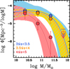 |
Fig. 6. Evolution in the SMF of passive galaxies from z = 5 to z = 3. The points, lines, and shaded regions follow those of Fig. 5. |
With the aim to understand the relative abundance of passive galaxies, we computed the SMF for the entire population. The results are shown in Fig. 7 (grey stepwise points and grey Schechter fits). We also show several SMF for the entire galaxy population taken from the literature (Ilbert et al. 2013; Duncan et al. 2014; Grazian et al. 2015; Davidzon et al. 2017; McLeod et al. 2021). Different fields, photometric quality, sample selections, methodology, and corrections for incompleteness are responsible for the large spread in the SMF observed at such high redshifts. For this reason, for a fair comparison with the passive population, instead of using a reference SMF from the literature we decided to recompute the SMF for all CANDELS H < 27 galaxies using the very same method applied to the passive candidates. We note that our estimates tend to be on the upper envelope of the distribution of the various results from the literature. This is a consequence of our choice to include AGNs in the sample.
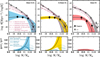 |
Fig. 7. Upper panels: SMF of passive candidates (black circles and curves, coloured shaded regions) vs. all H < 27 galaxies (grey squares and curves, shaded grey regions). The shaded regions indicate the regions at 68% confidence level considering the joint probability distribution function of the Schechter parameters. The dark red curves show SMF from the literature in similar, but not identical, redshift bins (as indicated in the legend), all scaled to the same IMF: Ilbert et al. (2013; long-dashed line), Duncan et al. (2014; dot long-dashed line), Grazian et al. (2015; dotted line), Davidzon et al. (2017; dashed line), and McLeod et al. (2021; dot short-dashed line). Lower panels: ratio of the passive and global Schechter functions. The shaded area and solid curve show the mass range where the comparison is meaningful (i.e. not affected by paucity of galaxies nor extrapolated due to the lack of observational data). We also show the passive fractions published by Davidzon et al. (2017; narrow-spaced shaded area) and Muzzin et al. (2013; wide-spaced shaded area), and the ratio of the passive to the total SMF of McLeod et al. (2021; dot dashed line). |
While at z < 4 the massive tail of the SMF of passive and all galaxies are rather similar, they diverge below ∼1011 M⊙. The lower panels of Fig. 7 show the ratio of the passive to the global SMF (ϕpas/ϕtot). As expected, we observe a trend with stellar mass, wherein passive galaxies are more abundant at high masses relative to the global population. While making a negligible fraction of the total population at ∼1010 M⊙, z < 4 passive galaxies become dominant at large stellar masses. Although the associated uncertainty is too large to estimate a precise fraction, passive galaxies could make up to ∼30% of the total galaxy population at M ∼ 1011 M⊙ and more than 50% at larger masses. We note, however, that while the passive SMF is nicely fitted by a Schechter function at stellar masses between 1010 and 1011.5 M⊙, its shape is poorly constrained above this value. As a consequence of the paucity of such sources, larger surveys are needed to better constrain the high-mass tail of the passive SMF. Consistent with the pronounced evolution around z ∼ 4, the fraction of passive galaxies earlier than this epoch is very low. Even at the highest masses, passive galaxies constitute no more than a few percent of the total galaxy population at z > 4.
We finally estimated the SMD accounted for by passive galaxies at different epochs by integrating the best-fit Schechter functions reproducing their SMF. We integrated the SMF from 1010 M⊙ to 1013 M⊙ in order not to be affected by large extrapolations at low stellar masses. The results and associated 1σ uncertainties are shown in Fig. 8 as green points and the shaded area, while the shaded grey region represents the global population.
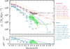 |
Fig. 8. Upper panel: evolution in the SMD of passive galaxies above 1010 M⊙ (green symbols and shaded area). As for comparison, the SMD of all H < 27 galaxies integrated above the same mass limit is also plotted (shaded grey region). In both cases, the shaded regions represent the 1σ uncertainty. The results are compared to a number of literature works, as listed in the legend, for passive galaxies (open blue symbols) and for the entire population (open dark red symbols and dot dashed line). The literature estimates and their mass integration limits have been scaled to a Salpeter IMF, when needed. The dashed orange and dotted red lines indicate the SMD derived by integrating SFR density from Hopkins & Beacom (2006) and Madau & Dickinson (2014), respectively, assuming a constant recycle fraction of 28%. The solid blue line shows the prediction for the SMD in passive galaxies by Renzini (2016). Lower panel: ratio of the mass density of passive galaxies to the overall galaxy population above 1010 M⊙ (solid green line and solid region). The passive fractions in terms of mass densities measured by Muzzin et al. (2013; triangles), Straatman et al. (2014; squares), Ilbert et al. (2013; 7-point stars), McLeod et al. (2021; pentagons), Mawatari et al. (2020; 5-point star), and predicted by Renzini (2016; solid line) are shown. |
An increase in the SMD of passive galaxies by a factor of 7 from z ∼ 5 to z ∼ 3 is observed. In the lower panel of Fig. 8 we show the passive fraction in terms of SMD, that is the ratio of the passive to the total SMD (ρpas/ρtot). Of the total mass assembled by redshift ∼3, 20−25% is accounted for by passive galaxies, while this fraction reduces to ∼5% at z > 4.
We verified that our results for the abundance of passive galaxies, in terms of their contribution to the SMF and SMD, remain unchanged when AGNs are excluded from the sample. The results may instead be affected by the inclusion of HST-dark galaxies, z ≳ 3 red galaxies that are undetected on the H-band image (Huang et al. 2011; Caputi et al. 2012; Wang et al. 2016, 2019; Alcalde Pampliega et al. 2019), whose abundance relative to the underlying H-detected red massive galaxy population increases with redshift and stellar mass. These objects are not included in our sample because of the H < 27 cut. Our simulation accounts for these objects to an extent that is impossible to quantify exactly because of the difficulty of mimicking their observed mass-to-light ratio distribution because they are not contained in the CANDELS catalogues. We can estimate an upper limit to their additional contribution to the overall statistics of high-z quiescent galaxies by correcting our passive and global SMF according to the results of Alcalde Pampliega et al. (2019). They estimated the contribution of HST-dark galaxies to a mass-selected sample in bins of redshift and stellar mass, and estimated that 30% of them are quiescent or post-starburst galaxies. While the effect of including HST-dark would be negligible at z < 4, at the highest redshifts the passive and global SMFs would increase by ∼0.2−0.3 (∼1) dex and ∼0.05 (∼0.1) dex, respectively, at intermediate (high) masses. This would however leave our results on the abundance of passive galaxies relative to the global population almost unaffected because of the already very low fraction of passive galaxies at z > 4. We note in any case that this is a conservative evaluation of the contribution of HST-dark galaxies to the passive fraction because of the less stringent definition of quiescent and post-starburst galaxy of Alcalde Pampliega et al. (2019) compared to that adopted by us.
Overall, despite the difficulties associated with the study of high-z passive galaxies, we can conclude that these sources are already in place in the young Universe. They make up a significant fraction (> 50%) of massive (M ≳ 1011 − 1011.5 M⊙) galaxies up to z = 4, and account for ∼20% of the total stellar mass formed by that time. On the contrary, only a few percent passive galaxies are observed earlier than this epoch. We are witnessing the emergence of the quiescent population, that is their passivization, in the redshift interval spanned by this work.
6. Comparison with the literature
6.1. Comparison with previous observations
At variance with other aspects of galaxy evolution over which a large consensus exists by now, the study of high-z passive galaxies, and in particular details such as their abundance, is still matter of debate, and current surveys have not found a final and joint solution yet. Early passive galaxies are rare sources, and several differences among the various analyses may be responsible for the variance among their results. Firstly, the photometric quality is crucial to detect these faint and elusive sources, and different filter combinations and depths affect the selection in a way that is not straightforward. Secondly, given the paucity of these sources, field-to-field variations may play an important role. Thirdly, different selection techniques may lead to different candidates, as discussed at length in M19. Finally, the methodology adopted to compute the SMF and the correction for observational incompleteness are essential ingredients in the analysis, as discussed in the following.
In this section, we compare our findings with the few previous works that analyse the SMF of passive galaxies at similar redshifts. In Fig. 5 we plot the SMF of Davidzon et al. (2017) and Ichikawa & Matsuoka (2017), using the same redshift bins adopted by us, and the estimate of McLeod et al. (2021), covering a redshift space slightly larger than our first interval but equally centred at z ∼ 3.25. As for reference, we also plot the results of Muzzin et al. (2013) and Girelli et al. (2019), although their SMFs are estimated on redshift intervals not coincident with ours, making the comparison tricky. For this reason, we do not discuss their results in the following. As for the Ichikawa & Matsuoka (2017) results, we sum their estimate for passive and recently quenched galaxies. For Davidzon et al. (2017) and McLeod et al. (2021) we plot their Schechter fits, which include the correction for the Eddington bias. All these works selected passive galaxies through a colour selection (based on either observed or rest-frame colours). All of them, except the McLeod et al. (2021) results, are based on the shallower COSMOS field.
Our SMF of passive galaxies at z ∼ 3.25 nicely agrees with that of McLeod et al. (2021) at intermediate mass, and is marginally 1σ consistent with it at the high-mass end. This mismatch may be due to fluctuations in the relatively small area that we probed. Overall, although we find larger densities, given the different parent sample, sample selection, and methodology, the consistency is more than satisfactory. The SMF that we measured at z ∼ 3.25 and z ∼ 3.75 are higher than those of Davidzon et al. (2017) by a factor of ∼4 to ∼8 at the peak and by more than a decade at larger masses. At z < 4 the mismatch with Ichikawa & Matsuoka (2017) is a factor of ∼4 at the peak, while the massive tail is marginally consistent with our results. The agreement with the latter study improves at z > 4, where the two estimates are well consistent within the error bars.
In the lower panels Fig. 7 we compare the fraction of passive sources as a function of stellar mass (ϕpas/ϕtot) with previous works that are less prone to the systematics associated with the various SMFs. Once again, our results nicely agree with those of McLeod et al. (2021) at M < 1011 M⊙, but diverge at higher masses, even though these results remain consistent within the error bars. Our results are also consistent within the uncertainties with those of Davidzon et al. (2017), while we observe higher fractions than Muzzin et al. (2013).
The literature results on the SMD of passive galaxies show a very large variance, spanning more than an order of magnitude at the redshifts probed by this work. Our results tend to be on the upper envelope of the ranges spanned by previous works, and are consistent with the analyses of McLeod et al. (2021), Straatman et al. (2014), and Shahidi et al. (2020; Fig. 8). We note however that the integration limits are not always consistent. For example, McLeod et al. (2021) integrate down to a lower-mass limit, but their lower SMD is likely explained by their steeper SMF at low (mostly) and high stellar masses.
The integrated passive fraction (i.e. the ratio of the SMD of passive to all galaxies,  , shown in the lower panel of Fig. 8) is consistent with that reported by Muzzin et al. (2013) and McLeod et al. (2021) at z ∼ 3−3.5. Straatman et al. (2014) find a higher ratio of 34% that is still consistent with our estimate; the difference is likely explained by their higher integration limit. Indeed, passive galaxies are more abundant at large stellar masses (shown in Fig. 7). However, their higher value might also reflect their higher number density and could be explained by their shallower selection criterion (see discussion in M19). The constant decline in the quiescent fraction observed from the local Universe to high redshift could flatten at z ≳ 2−3, as suggested by Straatman et al. (2014), all the way to z ∼ 4, before dropping to zero at z > 5 (Mawatari et al. 2020).
The fact that we measure higher SMF is somewhat expected thanks to the overall better CANDELS photometric quality (compared to the analyses based on COSMOS) and to the selection technique adopted to single out passive sources. Our selection does conservatively reject non-secure sources, but at the same time it is able to identify candidates that are missed by colour selections at these redshifts (see Merlin et al. 2018 and M19 for an extensive discussion; see also Schreiber et al. 2018a; Deshmukh et al. 2018; Carnall et al. 2020 regarding the incompleteness of the UVJ colour selection).
A trend to select a larger number of passive sources was already observed in the number density by M19. The mismatch is however larger in this work and is larger than reported by other authors (Shahidi et al. 2020) because of the corrections applied for incompleteness by our method. While the majority of previous works (except McLeod et al. 2021) only correct the observed mass distribution for incompleteness in stellar mass due to the survey depth, our procedure also takes into account the intrinsic incompleteness in the passive selection. As explained in Sect. 4, we applied to the very same selection technique adopted to single out the passive candidates to the simulated galaxies. In this way, our procedure not only accounts for galaxies with a light-to-mass ratio that is too low to be detected by our survey, but also for those passive galaxies that are missed by the selection (i.e. not classified as passive) as a result of photometric noise and survey properties (in terms of relative depth of the various bands).
To assess the relative contribution of the observed number densities of passive galaxies and incompleteness corrections to the mismatch with respect to previous works, we compared the literature results to our simple mass counts per unit volume without applying any correction. The mismatch reduces by a factor of ∼2−3. Our observed SMFs are still above the results of Davidzon et al. (2017). They are consistent or below the SMF the McLeod et al. (2021), as expected, since they also correct for incompleteness. Finally, compared to the results of Ichikawa & Matsuoka (2017), they are consistent at the highest redshift and only 1−2σ above at z < 4. These findings are expected from the mismatch in the mere number of candidates found by Davidzon et al. (2017) and Ichikawa & Matsuoka (2017), compared to our sample, scaled by the relative areas. The passive selection of Davidzon et al. (2017) and Ichikawa & Matsuoka (2017) encompasses ∼8 and ∼3.5 times, respectively, fewer candidates than ours (∼1.4 times less at the highest redshifts; Ichikawa & Matsuoka 2017). We also compared the uncorrected SMD of passive galaxies with literature results and found that it is in line with the bulk of previous estimates. Overall, our higher SMF and SMD derive from a combination of a generally larger number of passive candidates and a more accurate correction for mass incompleteness, Eddington bias, and incompleteness in the passive selection.
At variance with the observations just discussed are the predictions of Renzini (2016). He estimated the SMD in passive and star-forming galaxies by combining the parameterization for the evolution in the SFR density from Madau & Dickinson (2014) with that of the sSFR (=SFR/M) for near MS galaxies of Peng et al. (2010), assuming a unitary slope for the MS. The obtained SMD for the passive population is a factor of 2 to 5 above our measurements. His prediction for the passive fraction, shown in the lower panel of Fig. 8, is also higher than our observational data by a similar factor. In his empirical description, passive galaxies start dominating over the star-forming population at z > 3. We note, however, that these predictions are somewhat indirect and rely on the assumptions mentioned above as well as on the consistency between measurements of SFR and stellar mass, as discussed in the paper. Moreover, the definition of passive galaxies is not entirely consistent with ours, as Renzini (2016) defines as passive all sources with sSFR ≪ sSFRMS, including parts of star-forming galaxies such as quenched bulges and stellar haloes, so a higher abundance of passive sources is expected. On the other side, his method has the advantage of not being affected by incompleteness in the selection of passive candidates.
6.2. Comparison with theoretical predictions
To put our results in a broader context and understand how they fit the current theoretical scenario, we compared them with the predictions of one semi-analytic model (the PANDA model; Menci et al. 2014) and four hydrodynamic simulations (ILLUSTRIS-TNG100 and -TNG300; Pillepich et al. 2018a; Nelson et al. 2019, EAGLE; Schaye et al. 2015, and SIMBA; Davé et al. 2019).
6.2.1. The models
The model of Menci et al. (2014) is an improved version of the semi-analytic model of Menci et al. (2006, 2008). This model connects the baryonic processes (gas cooling, star formation, and supernova feedback) to the merging histories of the dark matter haloes computed by means of a Monte Carlo simulation within a cosmological framework. The AGN activity is triggered by galaxy interactions and, in this latest version, by disk instability. The description of AGN feedback is updated by implementing the 2D modelling for the expansion of AGN-driven shocks (Menci et al. 2019). This model adopts a Salpeter IMF.
ILLUSTRIS-TNG100 and -TNG300 exploit the moving mesh code AREPO (Springel 2010) and simulate volumes of 100 and 300 co-moving megaparsec on each side (110.73 and 302.63 Mpc3) with baryonic mass resolution of 1.4 × 10⁶ and 1.1 × 10⁷ M⊙, respectively. The EAGLE model is a set of simulations based on an updated version of the N-body Tree-PM smoothed particle hydrodynamics code GADGET-3 (Springel et al. 2005). We used the run EagleRefL0100N1504, which simulates a volume of 1003 Mpc3 with baryonic mass resolution of 1.81 × 10⁶ M⊙. The SIMBA simulations utilize the Gizmo cosmological gravity plus hydrodynamics solver (Hopkins 2015, 2017) in its meshless finite mass (MFM) version. It has a volume of (100/h)3 Mpc3, where h = 0.68, with baryonic mass resolution of 1.82 × 10⁷ M⊙. All these models include baryonic sub-grid physics to simulate star and black hole formation, stellar and AGN feedback, and metal enrichment. They assume Chabrier IMF, and have been scaled to a Salpeter IMF by multiplying the stellar masses by 1.74 (Salimbeni et al. 2009).
6.2.2. Selection of model passive galaxies
Accurately simulating the entire observational selection with a forward modelling approach is extremely time consuming and will be addressed in a future work (Fortuni et al., in prep.). We therefore adopted a standard criterion to select model passive galaxies. One possibility would be to select passive galaxies based on their specific SFR, which is required to be lower than a given threshold. While a fixed cut of 10−11 yr−1 is widely adopted, it may be too conservative if applied to high redshift galaxies because it does not take the evolution of the typical SFR into account. For this reason, we adopted the time-evolving criterion used by Pacifici et al. (2016), Carnall et al. (2019, 2020), as well as applied by Shahidi et al. (2020) on theoretical models; that is sSFR < 0.2/tU, where tU is the age of the Universe at the galaxy redshift.
The ILLUSTRIS-TNG and EAGLE simulations release multiple estimates of stellar mass and SFRs, based on the physical region within which they are computed. We adopted the very same stellar masses and SFR as in our previous work (M19). For ILLUSTRIS-TNG they are defined within twice the half-mass radius, best reproducing the observations (see M19, Valentino et al. 2020; Shahidi et al. 2020). For the EAGLE model, we considered the aperture that is closest to 4 × R1/2, 100, where R1/2, 100 is the half-mass radius computed within 100 kpc. For SIMBA, we adopted the stellar masses and SFRs associated with all particles gravitationally bound to the dark matter halo, as these are the only available in the catalogue. We note that the aperture choice over which stellar masses and SFRs are computed may have a significant effect on the selection of model passive galaxies, especially at 2 < z < 3 and M > 1010.5 M⊙, as shown by Donnari et al. (2020). In the future, we plan to extend their work to higher redshifts and analyse the impact of different definitions of quenched galaxies, apertures, and averaging timescales for the SFR (Fortuni et al., in prep.).
6.2.3. Predicted SMF
We show the comparison of theoretical predictions for the SMF with observational results in Fig. 9. Error bars associated with the hydrodynamic simulations are based on Poissonian errors. In the semi-analytic model, the uncertainty is caused by the limited number of merger tree realizations. We computed the relative error as the Poissonian error on the number N of merger tree realizations, that is  , where N = 40. For the semi-analytic model, we also considered a systematic uncertainty, which we summed in quadrature to the Poissonian uncertainty. Model predictions depend mainly on two quantities: the effective cooling time of gas inside the galactic dark matter potential wells and the effectiveness of interactions triggering powerful starbursts at high redshifts. In the model, both of the above processes can be slightly tuned to improve the agreement with observations, provided that they remain consistent with the observed colour distribution of local galaxies. This degree of freedom is reflected in a factor ∼2.5 systematic uncertainty associated with the prediction of the abundance of passive galaxies at high redshift (z ≥ 3).
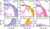 |
Fig. 9. Upper panels: observed SMF for passive galaxies (black points and curves, coloured solid shaded regions) compared to the theoretical predictions of the semi-analytic model of Menci et al. (2014) and the hydrodynamic simulations ILLUSTRIS-TNG100, ILLUSTRIS-TNG300, EAGLE, and SIMBA (see legend), scaled to a Salpeter IMF. The bins where the number of model passive galaxies is null are not shown. Lower panels: ratio of the passive to the global SMF. The coloured solid shaded area and solid curves show the observed fraction, as in Fig. 7. The open shaded regions show model predictions, according to the legend. |
The model of Menci et al. (2014) predicts an overabundance of low-mass passive galaxies and underestimates the massive tail of the SMF over the entire redshift range probed by this work. This is a well-known problem of galaxy formation models (Weinmann et al. 2012; Torrey et al. 2014; White et al. 2015; Somerville & Davé 2015). In a CDM scenario, dwarf galaxies form first, hence are characterized by old stellar populations, and feedback mechanisms effectively suppress their star formation. A partial solution to this problem was implemented by Henriques et al. (2017) through a revised feedback model tuned to fit the observed passive fraction at 0 < z < 3 (see also the comparison with the SMF for passive galaxies shown by Girelli et al. 2019).
The overestimate of the low-mass tail is not observed in ILLUSTRIS-TNG, where it has been suppressed by the introduction of a minimum stellar wind velocity (the so-called wind velocity floor; Pillepich et al. 2018a,b). The ILLUSTRIS-TNG300 simulation performs in an excellent manner at 3 < z < 3.5 and log M/M⊙ ≳ 10.7 and a still satisfactory way at higher redshift and high (log M/M⊙ ≳ 11−11.5) masses. However, it falls short of passive galaxies at low stellar masses compared to the observations. Donnari et al. (2020) report a very low fraction of M < 1010.5 M⊙ passive galaxies predicted by ILLUSTRIS-TNG300 at 0 < z < 3. They conclude that the ILLUSTRIS-TNG model captures the effect of AGN feedback in quenching massive galaxies (10.5 < log M/M⊙ < 11) very well, but needs some adjustment for the feedback mechanisms that regulate star formation in lower-mass galaxies at high redshift (e.g. stellar feedback). The inability of reproducing high-z passive galaxies (with the exception of the highest masses) is to be attributed to the still inefficient feedback. The ILLUSTRIS-TNG100 model very nicely reproduces the SMF of passive galaxies at z < 3.5 and log M/M⊙ ≳ 10.7 and it underpredicts the number of passive galaxies at lower masses. In the intermediate (high) redshift interval, however, it only predicts the correct abundance of passive sources at intermediate (high) stellar masses. At the high-mass end and intermediate redshifts, this could be due to the paucity of such systems, which can be under-represented in small simulated volumes; indeed, likely thanks to the larger volume, ILLUSTRIS-TNG300 is able to reproduce the massive tail of the SMF in the same redshift interval. With the exceptions of the mass and redshift bins where it predicts zero objects, ILLUSTRIS-TNG100 tends to overall predict a higher SMF than ILLUSTRIS-TNG300. This trend is also observed on the total SMF (Pillepich et al. 2018b), and it is due to the combination of volume effects and the limited numerical resolution, which is responsible for the lower number of particles exceeding the fixed density threshold above which stars can form.
An absence of massive passive galaxies as shown by TNG100 at intermediate redshifts is observed in the EAGLE and SIMBA simulations, which are both characterized by a similarly small volume. The SIMBA predictions confirm the trend already outlined in M19, where it turned out to be the model showing the most serious underestimate of the number density of passive galaxies at all redshifts above ∼1−1.5. While its predictions are similar to those of ILLUSTRIS-TNG300 at z > 3.5, it also underestimates the SMF at z < 3.5.
The most interesting comparison is however with EAGLE. This simulation very nicely reproduces the faint end of the SMF, but it predicts no quiescent galaxies at M ≥ 1011 M⊙ (an equally lack of massive passive sources is obtained, as expected, when using the more conservative cut sSFR < 10−11 yr−1, as in M19). This was somewhat unexpected, as in M19 we showed that EAGLE was the only hydrodynamic model, among those considered, that was able to reproduce the number density of M > 5 × 10⁹ M⊙ passive galaxies at z > 3.5. This implies that the number density alone is not a powerful observable because it does not encode information on the mass distribution of the sources. This results suggests that EAGLE might reproduce the abundance of high-z passive galaxies thanks to an overprediction of lower-mass sources. Our data, however, do not allow us to reliably measure the SMF below 1010 M⊙ to test this hypothesis.
The lower panels of Fig. 9 show the passive fraction as a function of stellar mass. Some of the models analysed match the observations at low masses, others show a good match at high masses, but none of the models are able to reproduce the observed passive fraction over the entire mass range. The two ILLUSTRIS-TNG simulations are consistent with the data in the lowest redshift interval, but are below the observations at the low-mass end. Similarly, they underpredict the passive fraction at higher redshift, with the exception of ILLUSTRIS-TNG100, which is consistent with the observations at 3.5 < z < 4 and log M/M⊙ ∼ 10.7. Conversely, over the entire redshift range probed, the predictions of EAGLE and of the model of Menci et al. (2014) agree with the observations at low masses, but no, or very few, passive galaxies are predicted at high masses. The SIMBA simulation predicts a very low fraction of passive galaxies roughly over the entire mass range.
6.2.4. Predicted SMD
Figure 10 shows the comparison between the observed and predicted SMD. For both models and data the SMD was computed above 1010.1 M⊙. The semi-analytic model of Menci et al. (2014) overpredicts the observed SMD owing to its steep shape at low masses, dominating the integral. Consistent with the comparison of the SMF, the two ILLUSTRIS simulations reproduce the SMD of passive galaxies at z ∼ 3, but underpredict it at higher redshifts. While the passive SMD according to SIMBA is always below the observations, EAGLE is marginally consistent at z ∼ 3 and nicely agrees with the data at z > 4. Despite its inability to reproduce the most massive passive galaxies, the SMD is dominated by the low-mass galaxies, and EAGLE turns out to be the only model among those considered that is able to nicely predict the faint end of the passive SMF at the highest redshifts. The lower panel of the same figure shows the ratio of the passive to total SMD. ILLUSTRIS-TNG100 very nicely reproduces the observed trend, and EAGLE is consistent within the uncertainties. The ILLUSTRIS-TNG300 and SIMBA simulations predict a fraction of mass in passive galaxies consistent with the observations at z < 3.5. Given the large observational uncertainty, the Menci et al. (2014) model as well as ILLUSTRIS-TNG300 and SIMBA at z > 3.5 are consistent with the data, although they systematically predict a negligible fraction of mass density accounted for by passive galaxies.
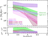 |
Fig. 10. Upper panel: evolution in the SMD of passive galaxies above 1010.1 M⊙ (green symbols and solid shaded area) compared to the theoretical predictions of the semi-analytic model of Menci et al. (2014) and the hydrodynamic simulations ILLUSTRIS-TNG100, ILLUSTRIS-TNG300, EAGLE, and SIMBA (see legend), scaled to a Salpeter IMF. Lower panel: ratio of the mass density of passive galaxies to the overall galaxy population above 1010.1 M⊙. The solid green line and solid region show the observed passive fraction, while the open shaded regions indicate model predictions, according to the legend. |
6.2.5. Conclusions
Overall, we observe a significant variation between the different models, even though their predictions roughly agree for the local SMF. In particular, the fact that none of the models analysed are able to reproduce the observed passive galaxies over the entire mass and redshift range suggests that these passive galaxies derive from a subtle combination of several physical processes. Analyses such as in this work will facilitate the validation of model recipes in a new and seemingly powerful way. In any case, the inability of the models to correctly reproduce the observed high-z passive galaxies denotes a still incomplete understanding of the physical mechanisms responsible for the formation of these galaxies, their rapid assembly and abrupt suppression of their star formation, and for galaxy evolution in general.
7. Predictions for future surveys
We extrapolated our SMFs to predict the intrinsic number of high-z passive galaxies expected in surveys carried our with future facilities, depending on their depth (H band limiting magnitude) and their area. Basically, from the typical observed mass-to-light ratio of our candidates as a function of their observed magnitude, we converted the limiting flux into a limiting stellar mass. We then integrated the SMF at the different redshifts above this limiting mass and rescaled to the relevant survey area.
We note that the number of galaxies predicted by extrapolating the SMF is by definition larger than the number of candidates we are able to select because of incompleteness of the actual surveys. As we discuss below, the availability of ancillary photometry, especially longward of the H band, and the choice of the specific selection technique affect the actual number of candidates.
The calculation is based on two main assumptions. The first is that the observed mass-to-light ratio (log M − H) versus H-band magnitude relation, well fitted by a linear slope at magnitudes brighter than 27, shows the same trend at fainter values. The second assumption is that the SMF, which we measure above 1010 M⊙, can be safely extrapolated to lower masses; we note that the faint-end slope was only fitted to the data in our lowest redshift bin, and it was kept fixed at higher redshifts. Both assumptions affect the predictions at magnitude deeper than 27, which is the magnitude cut of our selection. Indeed, H = 27 roughly corresponds to 1010 M⊙, where our SMFs are still safely based on the observations and do not suffer from strong uncertainties associated with their extrapolation. Predictions for surveys deeper than H = 27 should therefore been taken with caution.
Another important issue to account for is that the selection function for high-z passive galaxies is not simply based on the depth of the observations in the H band, but it depends in a complex way on the depth in other filters, in particular the K and IRAC CH1 and CH2 bands, as described in Sect. 2.1 and fully discussed in M19. This implies that, although future telescopes are expected to survey large sky areas down to very deep limiting H band fluxes, additional data will be needed to properly select the high-z passive galaxies predicted to be found in the observed sky regions. The selection efficiency will crucially depend on the availability of ancillary data. Our predictions can therefore be considered as upper limits to the expected number of candidates that will be detected by the future telescopes under consideration.
Keeping all these caveats in mind, the results of our calculation are shown in Fig. 11 and reported in Table 3. Given the large uncertainties associated with our SMFs, we only report the 68% confidence level intervals on the predicted number of passive galaxies. Since the slope of the SMF has been fixed at z > 3.5, the associated confidence regions are narrower than at lower redshift, and so are the uncertainties on our predictions.
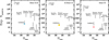 |
Fig. 11. Predicted number of passive galaxies at different redshifts expected at different flux limits in the areas surveyed by future facilities (see Table 3). The plotted range accounts for the uncertainty in the Schechter fits to the SMF (see text). The coloured boxes denote the number of candidates observed in CANDELS (this work). The predictions are by definition larger than the number of observed candidates owing to incompleteness of the actual surveys. |
Predicted number of passive galaxies at different redshifts expected at different flux limits, corresponding to different mass limits, in the areas surveyed by future facilities.
We first compared the expected number of passive sources in an area equal to the CANDELS area down to H = 27 to the number of candidates observed. As expected, the number of selected passive galaxies is lower than our predictions by a factor of ∼2−5. As discussed above, this mismatch is explained by the incompleteness in the observed sample. It is larger at higher redshift owing to the higher level of incompleteness for a given mass limit.
Besides a CANDELS-like survey, we considered the JWST Advanced Deep Extragalactic Survey (JADES), Euclid, and the Nancy Grace Roman Space Telescope. JADES1 is a JWST GTO programme, imaging with NIRCam 46 and 190 arcmin2 down to a limit of AB = 30.6 and 29.6, respectively, for the deep and medium survey, in the GOODS-S and GOODS-N fields. The Euclid deep and wide surveys will scan 40 and 15 000 deg2 down to a limiting depth of H = 24 and H = 26 (Laureijs et al. 2011), respectively. For the Nancy Grace Roman Space Telescope, we considered an ultra-deep survey reaching H = 30 over 1 deg2 (Koekemoer et al. 2019) and approximate depths of ∼28.9 and ∼27.5 over ∼5 and ∼9 deg2 for a deep and a medium survey, respectively (Hounsell et al. 2018).
Based on our predictions, given the scarcity of passive galaxies in the young Universe, the surveyed sky area turns out to be the key feature to perform statistical studies of this class of sources, more than the observing depth. Thanks to its much larger area, the Euclid deep survey, even though it is expected to be 1.5 and 3 mag shallower, will provide more candidates than the medium and deep surveys, respectively, carried out with the Nancy Grace Roman Space Telescope. The Euclid wide survey will further improve the statistics by a factor of ∼100, and by four orders of magnitude compared to what is now possible. We note, however, that we are simply predicting the number of candidates expected in a given sky area down to a given flux limit and not our capability in selecting these candidates. As discussed above, ancillary, deep enough data are needed at longer wavelength to complement optical and near-IR observations. Spitzer data from the SIMPLE survey (Damen et al. 2011) over the Extended CDF-South (∼0.5 deg2) and especially from the Euclid/WFIRST Spitzer Legacy Survey (covering 20 deg2, proposals IDs #13058 and #13153, PI P. Capak) will be of great help, but will not cover the entire sky areas that will be observed by Euclid and Roman. This will allow us to only detect a fraction of the predicted number of high-z passive candidates.
Despite its small field of view, hence the relatively small areas surveyed, in the next future JWST will be the only facility that will allow a self-standing selection of high-z passive galaxies, thanks to its red filters (> 2 μm) that will complement the H band observations to a similar depth. The JWST telescope will allow a much cleaner selection of the candidates (see Merlin et al. 2018), an easier and faster spectroscopical confirmation, and will extend the selection to even higher redshift because it has redder filters than CANDELS.
8. Summary
In this paper, we present a follow-up analysis of the passive galaxy candidates selected at z > 3 in the CANDELS fields by M19 through an accurate and ad hoc developed SED fitting technique. After confirming their passive nature by means of their sub-millimetre emission, probing the lack of ongoing star formation, we study the SMF of the passive population at 3 < z < 5. We summarize our results in the following.
We started by searching the ALMA archive for observations of our candidates. We found data for 77% of the sources located in the fields accessible by ALMA. Following the method presented in our previous work (S19), based on the comparison between ALMA predictions and the outcome of the SED fitting analysis, we could confirm the accuracy of the passive classification for 61% of the candidates on an individual basis at a 3σ confidence level. Since the available data are not deep enough to confirm or reject the rest of the candidates, we validated the population as being on average passive in a statistical sense, through stacking and by comparison with the location of the MS of star-forming galaxies at the same redshifts.
Once again (see S19), we confirmed the reliability and robustness of the photometric selection technique developed in Merlin et al. (2018). Assuming that it performs equally well on the sources for which no sub-millimetre information is available, we computed the SMF over the entire sample of 101 3 < z < 5 passive candidates using a stepwise approach. The latter has the advantage of taking photometric errors, mass and selection completeness issues, and the Eddington bias into account without any a posteriori correction.
We analysed the evolution in the SMF from z = 5 to z = 3 and compared it with the SMF of the total population. Despite the large associated uncertainties, we observe a strong evolution in the SMF around z ∼ 4, indicating that we are witnessing the emergence of the passive population at this epoch, that is we are looking at the epoch at which these galaxies become passive. Consistently, we observe an increase in the abundance of passive galaxies compared to the overall population at the same redshift. While quiescent galaxies are always below ≲10% at low (M ≲ 1010.5 M⊙) stellar masses, they can comprise a large fraction of the entire population (up to or more than 50%) at M > 1011 M⊙ and z < 4. On the other hand, their abundance remains low (≲10%) at z > 4. Integrating over M > 1010 M⊙, passive galaxies account for ∼20−25% of the total SMD at z = 3−4, and only ∼5% at earlier epochs. Current uncertainties on these numbers are however very large and prevent more accurate conclusions.
We compared our results with the literature and found a factor of 4 to 10 more passive sources than most previous observations with the exception of a couple of works consistent with our results within the uncertainties, at least in some of the redshift bins. This is owing to a combination of (a) the better quality of the CANDELS observations; (b) the very accurate selection technique developed by Merlin et al. (2018), which includes recently quenched galaxies often missed by colour-colour selections; and (c) the method adopted to calculate the SMF, which intrinsically accounts for mass and selection incompleteness, as well as the Eddington bias. We also compared our results with theoretical predictions. We found an overall agreement with at least some of the models considered, but also clear mismatches, denoting a still incomplete understanding of the physical processes responsible for the formation of these galaxies and for galaxy evolution in general.
The analysis of passive galaxies in the high-redshift Universe will be greatly improved by future facilities. Observations by JWST will improve their selection, and thanks to its spectroscopical capabilities will facilitate a faster confirmation and a deeper investigation of their physical processes. On the other hand, wide-field surveys with Euclid and the Nancy Grace Roman Space Telescope, complemented with ancillary optical and IR data, will be crucial to improve the statistical analysis of these rare sources. Depth, redder filters, and area will all combine to reduce the uncertainties currently affecting this kind of studies.
Acknowledgments
We thank the anonymous referee for the thorough and careful review of the manuscript. This paper makes use of the following ALMA data: 2012.1.00869.S, 2012.1.00173.S, 2013.1.00718.S, 2013.1.01292.S, 2013.1.00118.S, 2015.1.00242.S, 2015.1.00543.S, 2015.1.01074.S, 2015.1.00098.S, 2015.1.00870.S, 2015.1.00379.S, 2015.1.01495.S, 2016.1.01079.S. The IllustrisTNG simulations were undertaken with compute time awarded by the Gauss Centre for Supercomputing (GCS) under GCS Large-Scale Projects GCS-ILLU and GCS-DWAR on the GCS share of the supercomputer Hazel Hen at the High Performance Computing Center Stuttgart (HLRS), as well as on the machines of the Max Planck Computing and Data Facility (MPCDF) in Garching, Germany. We acknowledge the Virgo Consortium for making their simulation data available. The EAGLE simulations were performed using the DiRAC-2 facility at Durham, managed by the ICC, and the PRACE facility Curie based in France at TGCC, CEA, Bruyères-le-Châtel. We also thank Romeel Davé for help in using the SIMBA simulation data.
References
- Alcalde Pampliega, B., Pérez-González, P. G., Barro, G., et al. 2019, ApJ, 876, 135 [CrossRef] [Google Scholar]
- Barro, G., Pérez-González, P. G., Cava, A., et al. 2019, ApJS, 243, 22 [NASA ADS] [CrossRef] [Google Scholar]
- Bouwens, R. J., Illingworth, G. D., Franx, M., & Ford, H. 2008, ApJ, 686, 230 [NASA ADS] [CrossRef] [Google Scholar]
- Bruzual, G., & Charlot, S. 2003, MNRAS, 344, 1000 [NASA ADS] [CrossRef] [Google Scholar]
- Calzetti, D., Armus, L., Bohlin, R. C., et al. 2000, ApJ, 533, 682 [NASA ADS] [CrossRef] [Google Scholar]
- Cappelluti, N., Comastri, A., Fontana, A., et al. 2016, ApJ, 823, 95 [NASA ADS] [CrossRef] [Google Scholar]
- Caputi, K. I., Dunlop, J. S., McLure, R. J., et al. 2012, ApJ, 750, L20 [NASA ADS] [CrossRef] [Google Scholar]
- Carnall, A. C., McLure, R. J., Dunlop, J. S., et al. 2019, MNRAS, 490, 417 [Google Scholar]
- Carnall, A. C., Walker, S., McLure, R. J., et al. 2020, MNRAS, 496, 695 [Google Scholar]
- Castellano, M., Fontana, A., Paris, D., et al. 2010, A&A, 524, A28 [NASA ADS] [CrossRef] [EDP Sciences] [Google Scholar]
- Castellano, M., Fontana, A., Grazian, A., et al. 2012, A&A, 540, A39 [NASA ADS] [CrossRef] [EDP Sciences] [Google Scholar]
- Chary, R., & Elbaz, D. 2001, ApJ, 556, 562 [Google Scholar]
- Cimatti, A., Daddi, E., Renzini, A., et al. 2004, Nature, 430, 184 [Google Scholar]
- Dahlen, T., Mobasher, B., Faber, S. M., et al. 2013, ApJ, 775, 93 [Google Scholar]
- Dale, D. A., & Helou, G. 2002, ApJ, 576, 159 [NASA ADS] [CrossRef] [Google Scholar]
- Damen, M., Labbé, I., van Dokkum, P. G., et al. 2011, ApJ, 727, 1 [NASA ADS] [CrossRef] [Google Scholar]
- Davé, R., Anglés-Alcázar, D., Narayanan, D., et al. 2019, MNRAS, 486, 2827 [NASA ADS] [CrossRef] [Google Scholar]
- Davidzon, I., Ilbert, O., Laigle, C., et al. 2017, A&A, 605, A70 [NASA ADS] [CrossRef] [EDP Sciences] [Google Scholar]
- Deshmukh, S., Caputi, K. I., Ashby, M. L. N., et al. 2018, ApJ, 864, 166 [NASA ADS] [CrossRef] [Google Scholar]
- D’Eugenio, C., Daddi, E., Gobat, R., et al. 2020, A&A, submitted [arXiv:2012.02767] [Google Scholar]
- Donnari, M., Pillepich, A., Nelson, D., et al. 2020, MNRAS, submitted [arXiv:2008.00004] [Google Scholar]
- Driver, S. P., & Robotham, A. S. G. 2010, MNRAS, 407, 2131 [NASA ADS] [CrossRef] [Google Scholar]
- Duncan, K., Conselice, C. J., Mortlock, A., et al. 2014, MNRAS, 444, 2960 [NASA ADS] [CrossRef] [Google Scholar]
- Elbaz, D., Dickinson, M., Hwang, H. S., et al. 2011, A&A, 533, A119 [NASA ADS] [CrossRef] [EDP Sciences] [Google Scholar]
- Faisst, A. L., Fudamoto, Y., Oesch, P. A., et al. 2020, MNRAS, 498, 4192 [CrossRef] [Google Scholar]
- Feldmann, R., Hopkins, P. F., Quataert, E., Faucher-Giguère, C.-A., & Kereš, D. 2016, MNRAS, 458, L14 [CrossRef] [Google Scholar]
- Fontana, A., Pozzetti, L., Donnarumma, I., et al. 2004, A&A, 424, 23 [NASA ADS] [CrossRef] [EDP Sciences] [Google Scholar]
- Fontana, A., Santini, P., Grazian, A., et al. 2009, A&A, 501, 15 [NASA ADS] [CrossRef] [EDP Sciences] [Google Scholar]
- Fontana, A., Dunlop, J. S., Paris, D., et al. 2014, A&A, 570, A11 [NASA ADS] [CrossRef] [EDP Sciences] [Google Scholar]
- Forrest, B., Annunziatella, M., Wilson, G., et al. 2020a, ApJ, 890, L1 [CrossRef] [Google Scholar]
- Forrest, B., Marsan, Z. C., Annunziatella, M., et al. 2020b, ApJ, 903, 47 [CrossRef] [Google Scholar]
- Fujimoto, S., Ouchi, M., Shibuya, T., & Nagai, H. 2017, ApJ, 850, 83 [NASA ADS] [CrossRef] [Google Scholar]
- Galametz, A., Grazian, A., Fontana, A., et al. 2013, ApJS, 206, 10 [NASA ADS] [CrossRef] [Google Scholar]
- Genzel, R., Tacconi, L. J., Lutz, D., et al. 2015, ApJ, 800, 20 [Google Scholar]
- Girelli, G., Bolzonella, M., & Cimatti, A. 2019, A&A, 632, A80 [CrossRef] [EDP Sciences] [Google Scholar]
- Glazebrook, K., Schreiber, C., Labbé, I., et al. 2017, Nature, 544, 71 [NASA ADS] [CrossRef] [Google Scholar]
- Gobat, R., Daddi, E., Magdis, G., et al. 2018, Nat. Astron., 2, 239 [Google Scholar]
- Grazian, A., Salimbeni, S., Pentericci, L., et al. 2007, A&A, 465, 393 [NASA ADS] [CrossRef] [EDP Sciences] [Google Scholar]
- Grazian, A., Fontana, A., Santini, P., et al. 2015, A&A, 575, A96 [NASA ADS] [CrossRef] [EDP Sciences] [Google Scholar]
- Grogin, N. A., Kocevski, D. D., Faber, S. M., et al. 2011, ApJS, 197, 35 [NASA ADS] [CrossRef] [Google Scholar]
- Guo, Y., Ferguson, H. C., Giavalisco, M., et al. 2013, ApJS, 207, 24 [NASA ADS] [CrossRef] [Google Scholar]
- Henriques, B. M. B., White, S. D. M., Thomas, P. A., et al. 2017, MNRAS, 469, 2626 [Google Scholar]
- Hopkins, P. F. 2015, MNRAS, 450, 53 [NASA ADS] [CrossRef] [Google Scholar]
- Hopkins, P. F. 2017, ArXiv e-prints [arXiv:1712.01294] [Google Scholar]
- Hopkins, A. M., & Beacom, J. F. 2006, ApJ, 651, 142 [Google Scholar]
- Hounsell, R., Scolnic, D., Foley, R. J., et al. 2018, ApJ, 867, 23 [CrossRef] [Google Scholar]
- Huang, J. S., Zheng, X. Z., Rigopoulou, D., et al. 2011, ApJ, 742, L13 [NASA ADS] [CrossRef] [Google Scholar]
- Ichikawa, A., & Matsuoka, Y. 2017, ApJ, 843, L7 [CrossRef] [Google Scholar]
- Ilbert, O., McCracken, H. J., Le Fèvre, O., et al. 2013, A&A, 556, A55 [NASA ADS] [CrossRef] [EDP Sciences] [Google Scholar]
- Inami, H., Bacon, R., Brinchmann, J., et al. 2017, A&A, 608, A2 [NASA ADS] [CrossRef] [EDP Sciences] [Google Scholar]
- Kennicutt, R. C., & Evans, N. J. 2012, ARA&A, 50, 531 [NASA ADS] [CrossRef] [Google Scholar]
- Kodra, D. 2019, PhD Thesis, University of Pittsburgh [Google Scholar]
- Koekemoer, A. M., Faber, S. M., Ferguson, H. C., et al. 2011, ApJS, 197, 36 [NASA ADS] [CrossRef] [Google Scholar]
- Koekemoer, A., Foley, R. J., Spergel, D. N., et al. 2019, BAAS, 51, 550 [Google Scholar]
- Kriek, M., van Dokkum, P. G., Franx, M., et al. 2006, ApJ, 649, L71 [Google Scholar]
- Labbé, I., Huang, J., Franx, M., et al. 2005, ApJ, 624, L81 [NASA ADS] [CrossRef] [Google Scholar]
- Laureijs, R., Amiaux, J., Arduini, S., et al. 2011, ArXiv e-prints [arXiv:1110.3193] [Google Scholar]
- Lutz, D., Poglitsch, A., Altieri, B., et al. 2011, A&A, 532, A90 [NASA ADS] [CrossRef] [EDP Sciences] [Google Scholar]
- Madau, P., & Dickinson, M. 2014, ARA&A, 52, 415 [NASA ADS] [CrossRef] [Google Scholar]
- Magdis, G. E., Gobat, R., Valentino, F., et al. 2021, A&A, 647, A33 [CrossRef] [EDP Sciences] [Google Scholar]
- Magnelli, B., Lutz, D., Saintonge, A., et al. 2014, A&A, 561, A86 [NASA ADS] [CrossRef] [EDP Sciences] [Google Scholar]
- Mawatari, K., Inoue, A. K., Hashimoto, T., et al. 2020, ApJ, 889, 137 [NASA ADS] [CrossRef] [Google Scholar]
- McLeod, D. J., McLure, R. J., Dunlop, J. S., et al. 2021, MNRAS, 503, 4413 [CrossRef] [Google Scholar]
- Menci, N., Fontana, A., Giallongo, E., Grazian, A., & Salimbeni, S. 2006, ApJ, 647, 753 [NASA ADS] [CrossRef] [Google Scholar]
- Menci, N., Fiore, F., Puccetti, S., & Cavaliere, A. 2008, ApJ, 686, 219 [NASA ADS] [CrossRef] [Google Scholar]
- Menci, N., Gatti, M., Fiore, F., & Lamastra, A. 2014, A&A, 569, A37 [NASA ADS] [CrossRef] [EDP Sciences] [Google Scholar]
- Menci, N., Fiore, F., Feruglio, C., et al. 2019, ApJ, 877, 74 [NASA ADS] [CrossRef] [Google Scholar]
- Merlin, E., Fontana, A., Ferguson, H. C., et al. 2015, A&A, 582, A15 [NASA ADS] [CrossRef] [EDP Sciences] [Google Scholar]
- Merlin, E., Fontana, A., Castellano, M., et al. 2018, MNRAS, 473, 2098 [NASA ADS] [CrossRef] [Google Scholar]
- Merlin, E., Fortuni, F., Torelli, M., et al. 2019, MNRAS, 490, 3309 [NASA ADS] [CrossRef] [Google Scholar]
- Merlin, E., Castellano, M., Santini, P., et al. 2021, A&A, 649, A22 [CrossRef] [EDP Sciences] [Google Scholar]
- Michałowski, M. J., Watson, D., & Hjorth, J. 2010, ApJ, 712, 942 [NASA ADS] [CrossRef] [Google Scholar]
- Moster, B. P., Somerville, R. S., Newman, J. A., & Rix, H.-W. 2011, ApJ, 731, 113 [Google Scholar]
- Muzzin, A., Marchesini, D., Stefanon, M., et al. 2013, ApJS, 206, 8 [Google Scholar]
- Nayyeri, H., Mobasher, B., Hemmati, S., et al. 2014, ApJ, 794, 68 [NASA ADS] [CrossRef] [Google Scholar]
- Nayyeri, H., Hemmati, S., Mobasher, B., et al. 2017, ApJS, 228, 7 [NASA ADS] [CrossRef] [Google Scholar]
- Nelson, D., Springel, V., Pillepich, A., et al. 2019, Comput. Astrophys. Cosmol., 6, 2 [Google Scholar]
- Oliver, S. J., Bock, J., Altieri, B., et al. 2012, MNRAS, 424, 1614 [Google Scholar]
- Pacifici, C., Kassin, S. A., Weiner, B. J., et al. 2016, ApJ, 832, 79 [NASA ADS] [CrossRef] [Google Scholar]
- Peng, Y.-J., Lilly, S. J., Kovač, K., et al. 2010, ApJ, 721, 193 [NASA ADS] [CrossRef] [Google Scholar]
- Pillepich, A., Springel, V., Nelson, D., et al. 2018a, MNRAS, 473, 4077 [Google Scholar]
- Pillepich, A., Nelson, D., Hernquist, L., et al. 2018b, MNRAS, 475, 648 [NASA ADS] [CrossRef] [Google Scholar]
- Pope, A., Chary, R.-R., Alexander, D. M., et al. 2008, ApJ, 675, 1171 [Google Scholar]
- Prevot, M. L., Lequeux, J., Prevot, L., Maurice, E., & Rocca-Volmerange, B. 1984, A&A, 132, 389 [Google Scholar]
- Renzini, A. 2016, MNRAS, 460, L45 [NASA ADS] [CrossRef] [Google Scholar]
- Roseboom, I. G., Oliver, S. J., Kunz, M., et al. 2010, MNRAS, 409, 48 [NASA ADS] [CrossRef] [Google Scholar]
- Roseboom, I. G., Ivison, R. J., Greve, T. R., et al. 2012, MNRAS, 419, 2758 [NASA ADS] [CrossRef] [Google Scholar]
- Salimbeni, S., Fontana, A., Giallongo, E., et al. 2009, in American Institute of Physics Conference Series, eds. G. Giobbi, A. Tornambe, G. Raimondo, et al., 1111, 207 [Google Scholar]
- Salpeter, E. E. 1955, ApJ, 121, 161 [Google Scholar]
- Santini, P., Fontana, A., Grazian, A., et al. 2009, A&A, 504, 751 [NASA ADS] [CrossRef] [EDP Sciences] [Google Scholar]
- Santini, P., Rosario, D. J., Shao, L., et al. 2012, A&A, 540, A109 [NASA ADS] [CrossRef] [EDP Sciences] [Google Scholar]
- Santini, P., Ferguson, H. C., Fontana, A., et al. 2015, ApJ, 801, 97 [NASA ADS] [CrossRef] [Google Scholar]
- Santini, P., Fontana, A., Castellano, M., et al. 2017, ApJ, 847, 76 [NASA ADS] [CrossRef] [Google Scholar]
- Santini, P., Merlin, E., Fontana, A., et al. 2019, MNRAS, 486, 560 [NASA ADS] [CrossRef] [Google Scholar]
- Saracco, P., Longhetti, M., Severgnini, P., et al. 2005, MNRAS, 357, L40 [Google Scholar]
- Saracco, P., Marchesini, D., La Barbera, F., et al. 2020, ApJ, 905, 40 [CrossRef] [Google Scholar]
- Schaye, J., Crain, R. A., Bower, R. G., et al. 2015, MNRAS, 446, 521 [Google Scholar]
- Schreiber, C., Glazebrook, K., Nanayakkara, T., et al. 2018a, A&A, 618, A85 [NASA ADS] [CrossRef] [EDP Sciences] [Google Scholar]
- Schreiber, C., Elbaz, D., Pannella, M., et al. 2018b, A&A, 609, A30 [NASA ADS] [CrossRef] [EDP Sciences] [Google Scholar]
- Shahidi, A., Mobasher, B., Nayyeri, H., et al. 2020, ApJ, 897, 44 [CrossRef] [Google Scholar]
- Somerville, R. S., & Davé, R. 2015, ARA&A, 53, 51 [Google Scholar]
- Spitler, L. R., Straatman, C. M. S., Labbé, I., et al. 2014, ApJ, 787, L36 [NASA ADS] [CrossRef] [Google Scholar]
- Springel, V. 2010, MNRAS, 401, 791 [NASA ADS] [CrossRef] [Google Scholar]
- Springel, V., White, S. D. M., Jenkins, A., et al. 2005, Nature, 435, 629 [NASA ADS] [CrossRef] [PubMed] [Google Scholar]
- Stefanon, M., Yan, H., Mobasher, B., et al. 2017, ApJS, 229, 32 [NASA ADS] [CrossRef] [Google Scholar]
- Straatman, C. M. S., Labbé, I., Spitler, L. R., et al. 2014, ApJ, 783, L14 [NASA ADS] [CrossRef] [Google Scholar]
- Takeuchi, T. T., Yoshikawa, K., & Ishii, T. T. 2000, ApJS, 129, 1 [Google Scholar]
- Tanaka, M., Valentino, F., Toft, S., et al. 2019, ApJ, 885, L34 [Google Scholar]
- Tomczak, A. R., Quadri, R. F., Tran, K.-V. H., et al. 2014, ApJ, 783, 85 [NASA ADS] [CrossRef] [Google Scholar]
- Torrey, P., Vogelsberger, M., Genel, S., et al. 2014, MNRAS, 438, 1985 [NASA ADS] [CrossRef] [Google Scholar]
- Valentino, F., Tanaka, M., Davidzon, I., et al. 2020, ApJ, 889, 93 [Google Scholar]
- Vogelsberger, M., Genel, S., Springel, V., et al. 2014, MNRAS, 444, 1518 [NASA ADS] [CrossRef] [Google Scholar]
- Wang, T., Elbaz, D., Schreiber, C., et al. 2016, ApJ, 816, 84 [Google Scholar]
- Wang, T., Schreiber, C., Elbaz, D., et al. 2019, Nature, 572, 211 [Google Scholar]
- Weigel, A. K., Schawinski, K., & Bruderer, C. 2016, MNRAS, 459, 2150 [NASA ADS] [CrossRef] [Google Scholar]
- Weinmann, S. M., Pasquali, A., Oppenheimer, B. D., et al. 2012, MNRAS, 426, 2797 [NASA ADS] [CrossRef] [Google Scholar]
- White, C. E., Somerville, R. S., & Ferguson, H. C. 2015, ApJ, 799, 201 [NASA ADS] [CrossRef] [Google Scholar]
Appendix A: List of passive galaxy candidates
We list in Tables A.1–A.5 the passive candidates selected by Merlin et al. (2019) and used in this work (we do not include one source at z ∼ 6.7 as outside the redshift range probed) to compute the passive SMF. We report their redshift, H sband magnitude, and stellar masses. Tables A.1–A.3 show the candidates in GOODS-S, UDS, and COSMOS, respectively, and also report the sub-millimetre fluxes and inferred (limits on the) SFR for the sources having ALMA archival observations in Band 6 and 7. Tables A.4 and A.5 are for the GOODS-N and EGS fields, unobservable with ALMA. Table B.1 of Merlin et al. (2019) lists candidate positions, best-fit ages, and time since quiescence.
Passive galaxy candidates at 3 < z < 5 in the GOODS-S field.
Passive galaxy candidates at 3 < z < 5 in the UDS field.
Passive galaxy candidates at 3 < z < 5 in the COSMOS field.
Passive galaxy candidates at 3 < z < 5 in the GOODS-N field.
Passive galaxy candidates at 3 < z < 5 in the EGS field.
All Tables
Best-fit parameters and their 1σ uncertainties in the different redshift intervals derived from fitting the stepwise SMF with a Schechter function.
Predicted number of passive galaxies at different redshifts expected at different flux limits, corresponding to different mass limits, in the areas surveyed by future facilities.
All Figures
|
Fig. 1. Redshift distribution of the 3 ≤ z < 5 passive candidates used in the present analysis. Different colours show the counts in the various fields (see legend). The open black histogram shows the total sample. |
| In the text | |
|
Fig. 2. Mass distribution of the passive galaxies (open black histograms) compared to the overall galaxy population (shaded grey histograms) in different redshift bins. |
| In the text | |
|
Fig. 3. Distribution of the ratio of the stellar mass computed with τ-models to those with top-hat SFHs. The shaded grey histogram refers to the total population of H < 27 galaxies at 3 ≤ z < 5 with Mτ > 109.5 M⊙ in the five CANDELS fields, while the open black histogram shows the passive candidates. The numbers in the upper right corner show the mean and standard deviation of the two distributions. |
| In the text | |
|
Fig. 4. Location of the passive candidates observed by ALMA on a SFR-stellar mass diagram, in two redshift bins, based on their sub-millimetre SFR. The arrows represent 1σ upper limits on the SFR. The 1σ error bars on the stellar masses have been conservatively calculated by setting the redshift as a free parameter. The solid lines show the observed MS of Santini et al. (2017). The dotted lines are 1σ above and below the MS (estimated from the observed 0.3 dex scatter), while the dashed line is 3σ below the MS. Individual sources are shown in blue. Robust candidates (i.e. individually confirmed as passive at a 3σ confidence level) have been overplotted in light blue. The large orange symbols show the stacks in bins of stellar mass, denoted by the vertical dotted orange lines. |
| In the text | |
|
Fig. 5. SMF for passive galaxies in the five CANDELS fields. The solid black points show the stepwise results; the error bars account for Poissonian and cosmic variance uncertainties. The black curves show the Schechter fits and the coloured shaded areas indicate the regions at 68% confidence level considering the joint probability distribution function of the Schechter parameters. The open blue symbols and lines show the SMF for passive galaxies taken from the literature, scaled to a Salpeter IMF, in the same (or very similar) redshift bins (Ichikawa & Matsuoka 2017 as squares, Davidzon et al. 2017 as a dashed line, and McLeod et al. 2021 as a dot dashed line), and at slightly different redshifts (Muzzin et al. 2013 as triangles and Girelli et al. 2019 as 6-point stars). |
| In the text | |
|
Fig. 6. Evolution in the SMF of passive galaxies from z = 5 to z = 3. The points, lines, and shaded regions follow those of Fig. 5. |
| In the text | |
|
Fig. 7. Upper panels: SMF of passive candidates (black circles and curves, coloured shaded regions) vs. all H < 27 galaxies (grey squares and curves, shaded grey regions). The shaded regions indicate the regions at 68% confidence level considering the joint probability distribution function of the Schechter parameters. The dark red curves show SMF from the literature in similar, but not identical, redshift bins (as indicated in the legend), all scaled to the same IMF: Ilbert et al. (2013; long-dashed line), Duncan et al. (2014; dot long-dashed line), Grazian et al. (2015; dotted line), Davidzon et al. (2017; dashed line), and McLeod et al. (2021; dot short-dashed line). Lower panels: ratio of the passive and global Schechter functions. The shaded area and solid curve show the mass range where the comparison is meaningful (i.e. not affected by paucity of galaxies nor extrapolated due to the lack of observational data). We also show the passive fractions published by Davidzon et al. (2017; narrow-spaced shaded area) and Muzzin et al. (2013; wide-spaced shaded area), and the ratio of the passive to the total SMF of McLeod et al. (2021; dot dashed line). |
| In the text | |
|
Fig. 8. Upper panel: evolution in the SMD of passive galaxies above 1010 M⊙ (green symbols and shaded area). As for comparison, the SMD of all H < 27 galaxies integrated above the same mass limit is also plotted (shaded grey region). In both cases, the shaded regions represent the 1σ uncertainty. The results are compared to a number of literature works, as listed in the legend, for passive galaxies (open blue symbols) and for the entire population (open dark red symbols and dot dashed line). The literature estimates and their mass integration limits have been scaled to a Salpeter IMF, when needed. The dashed orange and dotted red lines indicate the SMD derived by integrating SFR density from Hopkins & Beacom (2006) and Madau & Dickinson (2014), respectively, assuming a constant recycle fraction of 28%. The solid blue line shows the prediction for the SMD in passive galaxies by Renzini (2016). Lower panel: ratio of the mass density of passive galaxies to the overall galaxy population above 1010 M⊙ (solid green line and solid region). The passive fractions in terms of mass densities measured by Muzzin et al. (2013; triangles), Straatman et al. (2014; squares), Ilbert et al. (2013; 7-point stars), McLeod et al. (2021; pentagons), Mawatari et al. (2020; 5-point star), and predicted by Renzini (2016; solid line) are shown. |
| In the text | |
|
Fig. 9. Upper panels: observed SMF for passive galaxies (black points and curves, coloured solid shaded regions) compared to the theoretical predictions of the semi-analytic model of Menci et al. (2014) and the hydrodynamic simulations ILLUSTRIS-TNG100, ILLUSTRIS-TNG300, EAGLE, and SIMBA (see legend), scaled to a Salpeter IMF. The bins where the number of model passive galaxies is null are not shown. Lower panels: ratio of the passive to the global SMF. The coloured solid shaded area and solid curves show the observed fraction, as in Fig. 7. The open shaded regions show model predictions, according to the legend. |
| In the text | |
|
Fig. 10. Upper panel: evolution in the SMD of passive galaxies above 1010.1 M⊙ (green symbols and solid shaded area) compared to the theoretical predictions of the semi-analytic model of Menci et al. (2014) and the hydrodynamic simulations ILLUSTRIS-TNG100, ILLUSTRIS-TNG300, EAGLE, and SIMBA (see legend), scaled to a Salpeter IMF. Lower panel: ratio of the mass density of passive galaxies to the overall galaxy population above 1010.1 M⊙. The solid green line and solid region show the observed passive fraction, while the open shaded regions indicate model predictions, according to the legend. |
| In the text | |
|
Fig. 11. Predicted number of passive galaxies at different redshifts expected at different flux limits in the areas surveyed by future facilities (see Table 3). The plotted range accounts for the uncertainty in the Schechter fits to the SMF (see text). The coloured boxes denote the number of candidates observed in CANDELS (this work). The predictions are by definition larger than the number of observed candidates owing to incompleteness of the actual surveys. |
| In the text | |
Current usage metrics show cumulative count of Article Views (full-text article views including HTML views, PDF and ePub downloads, according to the available data) and Abstracts Views on Vision4Press platform.
Data correspond to usage on the plateform after 2015. The current usage metrics is available 48-96 hours after online publication and is updated daily on week days.
Initial download of the metrics may take a while.