| Issue |
A&A
Volume 651, July 2021
|
|
|---|---|---|
| Article Number | L5 | |
| Number of page(s) | 14 | |
| Section | Letters to the Editor | |
| DOI | https://doi.org/10.1051/0004-6361/202141051 | |
| Published online | 09 July 2021 | |
Letter to the Editor
A major asymmetric ice trap in a planet-forming disk
I. Formaldehyde and methanol
1
Physics & Astronomy Department, University of Victoria, 3800 Finnerty Road, Victoria, BC V8P 5C2, Canada
e-mail: astro@nienkevandermarel.com
2
Leiden Observatory, Leiden University, 2300 RA Leiden, The Netherlands
3
Max-Plank-Institut fur Extraterrestrische Physik, Giessenbachstraße 1, 85748 Garching, Germany
4
RIKEN Cluster for Pioneering Research, 2-1, Hirosawa, Wako-shi, Saitama 351-0198, Japan
Received:
12
April
2021
Accepted:
5
June
2021
Context. The chemistry of planet-forming disks sets the exoplanet atmosphere composition and the prebiotic molecular content. Dust traps are of particular importance as pebble growth and transport are crucial for setting the chemistry where giant planets form.
Aims. The asymmetric Oph IRS 48 dust trap located at 60 au radius provides a unique laboratory for studying chemistry in pebble-concentrated environments in warm Herbig disks with gas-to-dust ratios as low as 0.01.
Methods. We use deep ALMA Band 7 line observations to search the IRS 48 disk for H2CO and CH3OH line emission, the first steps of complex organic chemistry.
Results. We report the detection of seven H2CO and six CH3OH lines with energy levels between 17 and 260 K. The line emission shows a crescent morphology, similar to the dust continuum, suggesting that the icy pebbles play an important role in the delivery of these molecules. Rotational diagrams and line ratios indicate that both molecules originate from warm molecular regions in the disk with temperatures > 100 K and column densities ∼1014 cm−2 or a fractional abundance of ∼10−8 and with H2CO/CH3OH ∼0.2, indicative of ice chemistry. Based on arguments from a physical-chemical model with low gas-to-dust ratios, we propose a scenario where the dust trap provides a huge icy grain reservoir in the disk midplane, or an ‘ice trap’, which can result in high gas-phase abundances of warm complex organic molecules through efficient vertical mixing.
Conclusions. This is the first time that complex organic molecules have been clearly linked to the presence of a dust trap. These results demonstrate the importance of including dust evolution and vertical transport in chemical disk models as icy dust concentrations provide important reservoirs for complex organic chemistry in disks.
Key words: astrochemistry / protoplanetary disks
© ESO 2021
1. Introduction
Protoplanetary disks around young stars are the cradles of planets, and the chemical composition in these disks sets the exoplanet atmospheric composition and the formation of prebiotic molecules on their surfaces (Ehrenfreund & Charnley 2000; Öberg & Bergin 2021). So far, mostly simple molecules have been detected in disks (e.g., Dutrey et al. 1997; Thi et al. 2004; Öberg et al. 2010, 2015; Walsh et al. 2016), and their abundances are set by photodissociation in the surface layers and by freeze-out in the midplane (Bergin et al. 2007). Complex organic molecules (COMs) may be present but are expected to be mostly locked up in ices. CO ice chemistry is crucial for the formation of COMs that can be thermally released into the gas phase (Herbst & van Dishoeck 2009). For Herbig disks, COMs cannot form in situ since they are warm and lack a large CO-ice reservoir (Agúndez et al. 2018). Surprisingly, CH3OH was recently detected in the Herbig disk HD100546 (Booth et al. 2021). This detection can be understood when CH3OH ice is inherited from earlier stages, followed by radial transport and sublimation at its ice line. Pebble growth and transport are known to play an important role in the chemical composition of disks and resulting exoplanet atmospheres (Cridland et al. 2017; Krijt et al. 2020). The connection between pebbles and ice chemistry can be studied directly in so-called dust traps (concentrations of dust grains), which may possibly reveal a much richer chemistry since dust rings are colder in the midplane (Alarcón et al. 2020), while exposed dust cavity walls can reveal sublimated midplane products (Cleeves et al. 2011; Mulders et al. 2011).
Dust traps are thought to be the main explanation for the observed narrow dust rings and asymmetries in high-resolution Atacama Large Millimeter/submillimeter Array (ALMA) observations, which also reveal a segregation between gas and dust (e.g., van der Marel et al. 2013; Pérez et al. 2014; Andrews et al. 2018). Pressure bumps at gap edges trap larger dust grains due to drag forces between gas and dust (Weidenschilling 1977), which can explain the appearance of dust rings in protoplanetary disks as the dust is prevented from drifting inwards (Pinilla et al. 2012a). In some cases, the pressure bump can become susceptible to the Rossby wave instability and form long-lived vortices (Barge & Sommeria 1995), which trap the dust in the azimuthal direction. The Herbig disk Oph IRS 48 is a textbook example of such a dust trap, showing an asymmetric dust concentration south of the star (van der Marel et al. 2013, 2015), and thus an ideal target for studying complex organic chemistry in a pebble-concentrated environment.
The presence of warm H2CO in the IRS 48 disk was discovered by van der Marel et al. (2014). H2CO is a precursor of more complex organic molecules, such as CH3OH, through CO ice hydrogenation (e.g., Watanabe & Kouchi 2002; Fuchs et al. 2009). The morphology appeared to be co-spatial with the dust crescent, but the detection was tentative. CH3OH was not detected in this work, but upper limits were derived. The H2CO/CH3OH abundance ratio can be used as a tracer of the formation mechanism (Garrod et al. 2006) since CH3OH can only be formed efficiently through ice chemistry, whereas H2CO has both an ice- and gas-phase route (e.g., Walsh et al. 2014). Gas-phase-dominated H2CO formation implies a ratio > 1 and ice-phase a ratio < 1. However, the derived H2CO/CH3OH ratio from van der Marel et al. (2014) of ≳0.3 was inconclusive regarding the formation mechanism. Whereas H2CO has been routinely detected in a range of protoplanetary disks (e.g., Pegues et al. 2020), CH3OH has only been detected in the TW Hya disk (Walsh et al. 2016), the young IRAS04302 disk (Podio et al. 2020) and outburst disk V883 Ori (van ’t Hoff et al. 2018; Lee et al. 2019), and, recently, in the Herbig disk HD100546 (Booth et al. 2021).
In this work we present the detection of multiple CH3OH and H2CO transitions in the IRS 48 system. It is only the second Herbig disk with observed COMs, and it is the first disk where the COM production can be linked directly to the dust trap.
2. Observations
Oph IRS 48 is an A0 star located in the Ophiuchus cloud at a distance of 135 pc (Gaia Collaboration 2018). This disk, inclined at 50°, shows an asymmetric millimetre-dust concentration at 60 au, in contrast with a full ring in gas, as well as small dust grains (van der Marel et al. 2013), and it has an estimated gas disk mass of only 0.6 MJup (van der Marel et al. 2016). IRS 48 was observed using ALMA in Band 7 in polarization mode in Cycle 5 in August 2018 (2017.1.00834.S, PI: Adriana Pohl). The continuum polarization data are presented by Ohashi et al. (2020), and the main calibration and reduction process is described in detail in that work. The total on-source integration time was 89 minutes. The continuum was subtracted in the uv-plane using the CASA task uvcontsub with a first order polynomial. The spectral setup contains four spectral windows, at 349.7, 351.5, 361.6, and 363.5 GHz, with a bandwidth of 1875 GHz in each window and a channel width of 1953 kHz, or ∼1.6 km s−1.
Seven H2CO and six CH3OH transitions were identified using the matched-filter technique (Loomis et al. 2018), listed in Table 1, for Eu levels between 17 and 260 K. H2CO transitions are identified as ortho (o-) and para (p-) transitions, respectively. Each line was imaged using the tclean task at the channel resolution using natural weighting. The final channel cubes have a beam size of 0.63 × 0.50″ and an rms noise of σrms ∼ 1.2 mJy beam−1 channel−1. The brightest lines (H2CO 50, 5 − 40, 4 and CH3OH 40, 4 − 31, 3) were also imaged using Briggs weighting with a robust of 0.5 for a resolution of 0.55 × 0.44″. Spectra were extracted from the naturally weighted cubes using Keplerian masking (using d = 135 pc, i = 50°, and M* = 2.0 M⊙) and are presented in Fig. A.1. All cubes show a clear Keplerian pattern along the southern part of the disk. Some lines are located adjacent to other lines (i.e., the H2CO 53, 3 − 43, 2 and 53, 2 − 43, 1 transitions), so line wings overlap in two channels.
Detected molecular lines, line properties, and disk-integrated fluxes.
The disk-integrated spectra are resolved even at our low spectral resolution, ranging from −2 to 12 km s−1 with vsource = 4.55 km s−1. The CH3OH lines appear to have somewhat more prominent line wings (corresponding to an inner 30 au radius) than the H2CO lines. The spectra were integrated over the entire individual profiles (avoiding overlap with adjacent features), and the disk-integrated fluxes are reported in Table 1. The H2CO 54, 2 − 44, 1 and 54, 1 − 44, 0 fluxes were computed by dividing their shared flux by two. The integrated fluxes were detected with a range between 5 and 42σint, with σint ∼ 20 mJy km s−1, whereas the calibration uncertainty was 10%.
Zero-moment maps were created using Keplerian masking and are presented in Fig. A.2. The central position was set at J2000 16h27m37.180s, −24° 30′35.48″, based on Gaia Data Release 2 (Gaia Collaboration 2018). Spectra and moment maps of the two brightest lines are presented in Fig. 1.
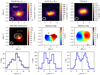 |
Fig. 1. Overview of the brightest H2CO and CH3OH lines using Briggs weighting, the 336 GHz continuum, and the 13CO 6–5 map, with a similar beam size for comparison. Top row: zero-moment maps, middle row: continuum and first-moment maps, and bottom row: disk-integrated spectra. The micron-sized grain distribution as traced by 19 μm VISIR data (Geers et al. 2007) is indicated in the continuum image. The source velocity is indicated by a vertical dotted line. The grey shades indicate the noise levels in the spectra. |
3. Results
Both H2CO and CH3OH lines are firmly detected. IRS 48 is the second known Herbig disk with a detection of CH3OH, following HD 100546 (Booth et al. 2021). It is immediately clear that both molecules follow the dust trap morphology (Fig. 1); this is in contrast with 13CO, which, just like the small grains, shows a full disk ring (van der Marel et al. 2013). This confirms the suggested location of the H2CO emission in van der Marel et al. (2014).
Figure 1 presents the data for the two brightest line transitions: the H2CO 51, 5 − 41, 4 and the CH3OH 40, 4 − 30, 3 lines. The maps were compared with the 355 GHz continuum from the same dataset and with the 13CO 6–5 intensity maps. The 13CO data were taken from van der Marel et al. (2016) and imaged using uv-tapering for a similar beam size as that of the Band 7 data presented here. The first-moment maps of the H2CO and CH3OH emission are consistent with Keplerian motion along the southern half of the disk.
A comparison between the images in both the radial and azimuthal directions is presented in Fig. 2. The profiles were extracted by de-projecting the zero-moment maps, assuming a position angle of 100° and an inclination of 50° (Bruderer et al. 2014). The azimuthal profile was extracted at the dust peak radius of 62 au with a radial width of 60 au and the radial profile at the peak ϕ of 192° east-of-north with an azimuthal width of 100°. For 13CO, the data were extracted around the peak radius of 35 au and the peak ϕ of 269°.
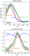 |
Fig. 2. Radially and azimuthally averaged profiles of the brightest H2CO and CH3OH lines from the Briggs-weighted images, combined with the profiles from 13CO 6–5 and the 355 GHz continuum imaged at the same beam size of 0.55 × 0.44″. |
The azimuthal profiles show that H2CO is azimuthally more extended than CH3OH and trails the dust trap, whereas CH3OH is similar in width to the continuum emission. In contrast, the 13CO emission is present along the entire ring, with a dip around the continuum peak due to continuum over-subtraction (the Band 9 continuum peak is azimuthally shifted with respect to the Band 7 continuum due to the different grain sizes traced). The Band 7 line data presented here are only moderately affected by continuum over-subtraction. Radially, the H2CO profile is co-spatial with the continuum emission, although the emission remains radially unresolved. In contrast, the CH3OH profile appears somewhat further extended outwards and, based on the line wings, also inwards. The 13CO emission peaks radially inside the dust continuum peak.
4. Analysis
With multiple line transitions it is possible to derive the column density and excitation temperature for both molecules under the assumption of local thermodynamic equilibrium (LTE) and optically thin emission (or a correction for optical depth). The optical depth was determined first using the expected emission from the emitting area. As the zero-moment maps of H2CO and CH3OH are marginally resolved, the emitting area cannot be reliably determined from these images. Instead, the emitting area was determined using the high-resolution (0.18 × 0.14″) Band 7 continuum image (Francis & van der Marel 2020, and Fig. A.3), with the underlying assumption that the H2CO and CH3OH emission follow the morphology of the dust crescent. Although the H2CO emission is azimuthally more extended than the continuum, the difference is marginal (∼20% in the convolved images) and can be ignored. The emitting area of the high-resolution continuum is 1.4 × 10⁻¹¹ sr with a 5σ threshold.
Using this emitting area, the optical depth, τ, and the column densities of individual levels, Nu, were estimated following the excitation equations in Loomis et al. (2018). All lines are optically thin with τ < 0.1 for T > 100 K. The ortho-to-para ratio of H2CO in the degeneracies and partition functions was taken to be three, and the A/E ratio of CH3OH to be one. The column density NT and temperature Trot were estimated by fitting the rotational diagrams using the emcee package to compute the posterior distributions (Foreman-Mackey et al. 2013), assuming optically thin emission. Our best-fit results are shown in Fig. B.1 and indicate an average column density of 7.7 ± 0.5 × 1013 cm−2 and 4.9 ± 0.2 × 1014 cm−2 and a rotational temperature of  and
and  K for H2CO and CH3OH, respectively (see Fig. B.2). This implies that the temperature of H2CO is higher than that of CH3OH; the abundance ratio H2CO/CH3OH is 0.16 ± 0.01, much lower than what is found for other disks (Booth et al. 2021), which is suggestive of ice-dominated chemistry. However, it is possible that the transitions trace multiple regimes with different temperatures in the disk. Furthermore, the ortho-to-para ratio obtained by fitting the ortho and para lines separately is < 3; this potentially points to an ice formation route as well (Terwisscha van Scheltinga et al. 2021) but could also be caused by optical depth (see Appendix B). The gas surface density derived by van der Marel et al. (2016) at 60 au radius corresponds to NH2 ∼ 1.6 × 1022 cm−2, so the relative abundances of H2CO and CH3OH are ∼10−8 with respect to H2, consistent with previous estimates by van der Marel et al. (2014).
The excitation temperature (rotational temperature) is equal to the kinetic temperature under the assumption of LTE at high densities. H2CO lines are particularly good diagnostics of kinetic temperature since radiative transitions are not allowed between the different Kp ladders. The relative populations of those ladders are therefore dominated by collisions only (Mangum & Wootten 1993; van Dishoeck et al. 1993). The LTE assumption and corresponding kinetic temperature can be tested using a calculation of the balance between excitation and de-excitation using RADEX (van der Tak et al. 2007). Collisional rate coefficients were taken from the LAMDA database1 for the individual molecules (Rabli & Flower 2010; Wiesenfeld & Faure 2013), as summarized in Schöier et al. (2005). We computed line ratios for a range of temperatures and H2 densities and a molecular column density of 1014 cm−2, shown in Fig. C.3, following van Dishoeck et al. (1995).
The H2 densities in the midplane and molecular layers of IRS 48 are ∼106−8 cm−3 (Bruderer et al. 2014). In this regime, the line ratios are only sensitive to temperature, with typical inferred values of 200 ± 50 K for H2CO and 100 ± 20 K for CH3OH, confirming that the H2CO emission originates from a warmer layer (Fig. C.3).
5. Discussion and conclusions
The strong detection of CH3OH and its precursor H2CO in IRS 48 challenges current chemical disk models, which predict that Herbig disks cannot form COMs in situ due to their warmer midplane (Agúndez et al. 2018). IRS 48 is the second mature Herbig disk with a CH3OH detection, following HD100546 (Booth et al. 2021). The derived H2CO/CH3OH abundance ratio of ∼0.2 in IRS 48 indicates that ice chemistry must be the primary formation mechanism. The warm excitation temperatures, > 100 K, indicate that the emission does not originate from the disk midplane, which has a temperature of ∼70 K at 60 au (Bruderer et al. 2014). The continuum brightness temperature at 355 GHz is 27 K, providing a lower limit. Considering its rotational temperature, H2CO may originate from slightly higher layers than CH3OH.
An important clue for the origin of the COM chemistry in IRS 48 is the striking crescent morphology of the emission, which follows the shape of the dust continuum. The asymmetric dust continuum has been interpreted as a dust trap based on the comparison between large grains, small grains, and gas (van der Marel et al. 2013). The high degree of chemical complexity may thus be related to special physical conditions there. Large grains concentrate in a dust trap and grow efficiently to larger sizes due to the higher dust concentration and lower destructive collision efficiency (Weidenschilling 1977; Brauer et al. 2008; Pinilla et al. 2012b). Small grains are still continuously produced by fragmentation. The dust trap thus provides a large reservoir of icy dust grains; if these have been either radially transported from the outer part of the disk or inherited from the early, colder stages, they might be rich in ices (Krijt et al. 2020; Booth et al. 2021). The dust trap thus acts as an ‘ice trap’ of large icy dust grains, as previously suggested for TW Hya (Walsh et al. 2016). Considering typical interstellar ice abundances of CH3OH of 3 × 10⁻⁶ (Boogert et al. 2015) and model COM ice abundances in the disk midplane of ≥10−6 (Walsh et al. 2014), only a fraction of the ice content is sublimated.
The dust density distribution in the dust trap plays a crucial role here as dust grains limit the UV field penetration in the disk, lowering the dust and gas temperature (Bruderer et al. 2012). Ohashi et al. (2020) derived a dust surface density as high as 2–8 g cm−2 at the dust trap radius based on polarization continuum measurements and constraints from the centimetre emission in IRS 48. This is well above the gas surface density of 0.07 g cm−2 derived from CO isotopologues and DALI modelling by van der Marel et al. (2016), implying a dust-to-gas ratio ≫1. Using a series of physical-chemical models with different dust surface densities, we estimated the temperature in the disk at the location of the dust trap. Two sets of models were run: first, only the dust density of the large grains in the midplane was increased (settled models), and second the dust density was increased throughout the column (full models). The details of the vertical and radial structure of the gas and dust of the models are described in Appendix C.
Figure 3 shows the midplane temperature profiles and the vertical gas temperature profiles at 65 au (away from the edge), based on the model output (Figs. C.1 and C.2). The gas temperature is coupled to the dust temperature in the midplane, up to z/r ≲ 0.15. Figure 3 demonstrates that the midplane temperature may fall as low as 40 K in the dust trap, well below the H2CO sublimation temperature of 66 K (Penteado et al. 2017). The temperature is unlikely to be below the CO freeze-out temperature of 22 K, so continuous formation of H2CO and CH3OH through CO ice hydrogenation is not possible. However, the dust trap contains a very large reservoir of icy grains. In order to sublimate, icy grains containing H2CO and CH3OH need to be vertically transported to the higher, warmer layers of the disk. The right panel in Fig. 3 shows that the temperature reaches > 100 K at a height of z/r ∼ 0.2 for the settled models in the emitting layer of H2CO and CH3OH. The full models reach temperatures of only 80 K, not high enough to explain the observed excitation temperatures, suggesting that the high dust concentration of large dust grains must be settled to the midplane. We note that the gas temperature in the warm molecular layer in IRS48 is estimated as 250–350 K from mid-J rotational CO lines (Fedele et al. 2016) and that the brightness temperature of the 13CO 6–5 line is as high as ∼200 K (van der Marel et al. 2016).
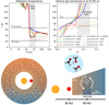 |
Fig. 3. Temperature structure and proposed scenario for the release of the COMs in the dust trap. Top left: radial dust temperature profiles of the midplane. Top right: vertical gas temperature profiles at 65 au, just inside the dust trap. Both temperature profiles are based on our physical-chemical DALI models, with different dust surface densities (Figs. C.1 and C.2). In the midplane, the gas temperature is equal to the dust temperature. The plots demonstrate that the dust trap provides sufficiently low temperatures for a COM ice reservoir in the settled midplane, whereas the temperatures in the emitting layer are sufficiently high to explain the derived excitation temperatures. Bottom: sketch of the proposed scenario for the complex organic chemistry in a dust trap based on this work. The blue-orange gradient indicates the predicted temperature structure in the disk, the large arrows the vertical and radial transport of the icy pebbles, and the small arrow the thermal desorption at the inner edge of the dust trap. |
This distribution of icy dust grains and molecules requires efficient vertical transport in the disk, which can be achieved by turbulent mixing (Semenov & Wiebe 2011). In addition, the dynamics of the vortex itself may play a role as both the vertical shear instability (Flock et al. 2020) and meridional flows (Meheut et al. 2010) in vortices increase the vertical mixing. The full scenario of the ice reservoir, mixing, and sublimation is summarized in the bottom panels of Fig. 3.
The morphology of the COM emission suggests that the combination of a concentration of icy dust pebbles and the irradiation of the cavity wall (resulting in a thin layer of thermal sublimation, as proposed by Cleeves et al. 2011) increases the chemical complexity in IRS 48. It is also important to point out that the COM emission is unlikely to trace an actual azimuthal gas over-density in the disk: considering the high S/N, the azimuthal contrast would have to be more than a factor of ten; such a contrast was not detected in the C18O 6–5 isotopologue emission (van der Marel et al. 2016), which is optically thin, considering the ratio of 4.3 ± 1.4 with the C17O flux measured by Bruderer et al. (2014).
The difference in azimuthal extent between H2CO and CH3OH could be explained by the lower desorption temperature of H2CO compared to CH3OH. This discrepancy cannot be explained by additional gas-phase chemistry production as this would result in H2CO emission along the entire ring. Formation by gas-phase chemistry cannot be excluded, but, due to the extreme dust trapping, the ice sublimation dominates the observable chemistry.
It is unclear whether the high dust-to-gas ratio environment and high COM abundances are unique to IRS 48. Pegues et al. (2020) and Facchini et al. (2021) derive H2CO column densities of ∼1012 cm−2 and low excitation temperatures of 20–30 K for a number of T Tauri disks, whereas for HD100546 the rotational temperature in the inner 50 au was derived as 50–100 K (Booth et al. 2021). All these T Tauri disks have radial dust traps, which also lead to dust concentrations smaller than the beam size of the COM observations. Interestingly, Pegues et al. (2020) find a higher column density of ∼1013 cm−2 for J1604−2130, the only disk in their sample for which the H2CO emission is more resolved radially, revealing the ring structure also seen in the continuum. As the inferred column densities rely on the assumed emitting area, the column densities in these works are lower limits and may be as high as in IRS 48. However, the high excitation temperatures of the COMs in IRS 48 require more efficient vertical transport, which may be due to the unique vortex properties.
IRS 48 is the first protoplanetary disk with a clear link between the morphology of the COM emission and the continuum. These results show the importance of taking dust traps into account in chemical disk models for the production of complex organic chemistry as well as for spatially resolving COMs in disks for comparison with the dust substructure.
Acknowledgments
We thank the referee for their thoughtful report, which has improved the clarity of the manuscript. We would also like to thank Wlad Lyra and Sebastiaan Krijt for useful discussions and Akimasa Kataoka for his help with the reduction of the data. N.M. acknowledges support from the Banting Postdoctoral Fellowships program, administered by the Government of Canada. ALMA is a partnership of ESO (representing its member states), NSF (USA) and NINS (Japan), together with NRC (Canada) and NSC and ASIAA (Taiwan) and KASI (Republic of Korea), in cooperation with the Republic of Chile. The Joint ALMA Observatory is operated by ESO, AUI/ NRAO and NAOJ. This paper makes use of the following ALMA data: 2017.1.00834.S.
References
- Agúndez, M., Roueff, E., Le Petit, F., & Le Bourlot, J. 2018, A&A, 616, A19 [NASA ADS] [CrossRef] [EDP Sciences] [Google Scholar]
- Alarcón, F., Teague, R., Zhang, K., Bergin, E. A., & Barraza-Alfaro, M. 2020, ApJ, 905, 68 [Google Scholar]
- Andrews, S. M., Wilner, D. J., Espaillat, C., et al. 2011, ApJ, 732, 42 [Google Scholar]
- Andrews, S. M., Huang, J., Pérez, L. M., et al. 2018, ApJ, 869, L41 [Google Scholar]
- Barge, P., & Sommeria, J. 1995, A&A, 295, L1 [NASA ADS] [Google Scholar]
- Bergin, E. A., Aikawa, Y., Blake, G. A., & van Dishoeck, E. F. 2007, Protostars and Planets V, 751 [Google Scholar]
- Boogert, A. C. A., Gerakines, P. A., & Whittet, D. C. B. 2015, ARA&A, 53, 541 [Google Scholar]
- Booth, A. S., Walsh, C., Terwisscha van Scheltinga, J., et al. 2021, Nat. Astron., 651, L6 [Google Scholar]
- Brauer, F., Dullemond, C. P., & Henning, T. 2008, A&A, 480, 859 [NASA ADS] [CrossRef] [EDP Sciences] [Google Scholar]
- Bruderer, S. 2013, A&A, 559, A46 [NASA ADS] [CrossRef] [EDP Sciences] [Google Scholar]
- Bruderer, S., van Dishoeck, E. F., Doty, S. D., & Herczeg, G. J. 2012, A&A, 541, A91 [NASA ADS] [CrossRef] [EDP Sciences] [Google Scholar]
- Bruderer, S., van der Marel, N., van Dishoeck, E. F., & van Kempen, T. A. 2014, A&A, 562, A26 [NASA ADS] [CrossRef] [EDP Sciences] [Google Scholar]
- Cleeves, L. I., Bergin, E. A., Bethell, T. J., et al. 2011, ApJ, 743, L2 [NASA ADS] [CrossRef] [Google Scholar]
- Cridland, A. J., Pudritz, R. E., & Birnstiel, T. 2017, MNRAS, 465, 3865 [Google Scholar]
- Dutrey, A., Guilloteau, S., & Guelin, M. 1997, A&A, 317, L55 [NASA ADS] [Google Scholar]
- Ehrenfreund, P., & Charnley, S. B. 2000, ARA&A, 38, 427 [Google Scholar]
- Facchini, S., Teague, R., Bae, J., et al. 2021, AJ, submitted [arXiv:2101.08369] [Google Scholar]
- Fedele, D., van Dishoeck, E. F., Kama, M., Bruderer, S., & Hogerheijde, M. R. 2016, A&A, 591, A95 [NASA ADS] [CrossRef] [EDP Sciences] [Google Scholar]
- Flock, M., Turner, N. J., Nelson, R. P., et al. 2020, ApJ, 897, 155 [CrossRef] [Google Scholar]
- Foreman-Mackey, D., Hogg, D. W., Lang, D., & Goodman, J. 2013, PASP, 125, 306 [Google Scholar]
- Francis, L., & van der Marel, N. 2020, ApJ, 892, 111 [Google Scholar]
- Fuchs, G. W., Cuppen, H. M., Ioppolo, S., et al. 2009, A&A, 505, 629 [NASA ADS] [CrossRef] [EDP Sciences] [Google Scholar]
- Gaia Collaboration (Brown, A. G. A., et al.) 2018, A&A, 616, A1 [NASA ADS] [CrossRef] [EDP Sciences] [Google Scholar]
- Garrod, R., Park, I. H., Caselli, P., & Herbst, E. 2006, Faraday Discussions, 133, 51 [Google Scholar]
- Geers, V. C., Pontoppidan, K. M., van Dishoeck, E. F., et al. 2007, A&A, 469, L35 [NASA ADS] [CrossRef] [EDP Sciences] [Google Scholar]
- Hama, T., Kouchi, A., & Watanabe, N. 2018, ApJ, 857, L13 [Google Scholar]
- Herbst, E., & van Dishoeck, E. F. 2009, ARA&A, 47, 427 [NASA ADS] [CrossRef] [Google Scholar]
- Kahane, C., Frerking, M. A., Langer, W. D., Encrenas, P., & Lucas, R. 1984, A&A, 137, 211 [Google Scholar]
- Krijt, S., Bosman, A. D., Zhang, K., et al. 2020, ApJ, 899, 134 [Google Scholar]
- Lee, J.-E., Lee, S., Baek, G., et al. 2019, Nat. Astron., 3, 314 [NASA ADS] [CrossRef] [Google Scholar]
- Loomis, R. A., Öberg, K. I., Andrews, S. M., et al. 2018, AJ, 155, 182 [NASA ADS] [CrossRef] [Google Scholar]
- Mangum, J. G., & Wootten, A. 1993, ApJS, 89, 123 [Google Scholar]
- Meheut, H., Casse, F., Varniere, P., & Tagger, M. 2010, A&A, 516, A31 [NASA ADS] [CrossRef] [EDP Sciences] [Google Scholar]
- Mulders, G. D., Waters, L. B. F. M., Dominik, C., et al. 2011, A&A, 531, A93 [NASA ADS] [CrossRef] [EDP Sciences] [Google Scholar]
- Öberg, K. I., & Bergin, E. A. 2021, Phys. Rep., 893, 1 [Google Scholar]
- Öberg, K. I., Qi, C., Fogel, J. K. J., et al. 2010, ApJ, 720, 480 [NASA ADS] [CrossRef] [Google Scholar]
- Öberg, K. I., Guzmán, V. V., Furuya, K., et al. 2015, Nature, 520, 198 [Google Scholar]
- Ohashi, S., Kataoka, A., van der Marel, N., et al. 2020, ApJ, 900, 81 [Google Scholar]
- Pegues, J., Öberg, K. I., Bergner, J. B., et al. 2020, ApJ, 890, 142 [CrossRef] [Google Scholar]
- Penteado, E. M., Walsh, C., & Cuppen, H. M. 2017, ApJ, 844, 71 [NASA ADS] [CrossRef] [Google Scholar]
- Pérez, L. M., Isella, A., Carpenter, J. M., & Chandler, C. J. 2014, ApJ, 783, L13 [NASA ADS] [CrossRef] [Google Scholar]
- Pinilla, P., Benisty, M., & Birnstiel, T. 2012a, A&A, 545, A81 [NASA ADS] [CrossRef] [EDP Sciences] [Google Scholar]
- Pinilla, P., Birnstiel, T., Ricci, L., et al. 2012b, A&A, 538, A114 [NASA ADS] [CrossRef] [EDP Sciences] [Google Scholar]
- Podio, L., Garufi, A., Codella, C., et al. 2020, A&A, 642, L7 [CrossRef] [EDP Sciences] [Google Scholar]
- Rabli, D., & Flower, D. R. 2010, MNRAS, 406, 95 [Google Scholar]
- Schöier, F. L., van der Tak, F. F. S., van Dishoeck, E. F., & Black, J. H. 2005, A&A, 432, 369 [NASA ADS] [CrossRef] [EDP Sciences] [Google Scholar]
- Semenov, D., & Wiebe, D. 2011, ApJS, 196, 25 [Google Scholar]
- Terwisscha van Scheltinga, J., Hogerheijde, M. R., Cleeves, L. I., et al. 2021, ApJ, 906, 111 [Google Scholar]
- Thi, W.-F., van Zadelhoff, G.-J., & van Dishoeck, E. F. 2004, A&A, 425, 955 [NASA ADS] [CrossRef] [EDP Sciences] [Google Scholar]
- van der Marel, N., van Dishoeck, E. F., Bruderer, S., et al. 2013, Science, 340, 1199 [Google Scholar]
- van der Marel, N., van Dishoeck, E. F., Bruderer, S., & van Kempen, T. A. 2014, A&A, 563, A113 [NASA ADS] [CrossRef] [EDP Sciences] [Google Scholar]
- van der Marel, N., Pinilla, P., Tobin, J., et al. 2015, ApJ, 810, L7 [Google Scholar]
- van der Marel, N., van Dishoeck, E. F., Bruderer, S., et al. 2016, A&A, 585, A58 [NASA ADS] [CrossRef] [EDP Sciences] [Google Scholar]
- van der Tak, F. F. S., Black, J. H., Schöier, F. L., Jansen, D. J., & van Dishoeck, E. F. 2007, A&A, 468, 627 [NASA ADS] [CrossRef] [EDP Sciences] [Google Scholar]
- van Dishoeck, E. F., Blake, G. A., Draine, B. T., & Lunine, J. I. 1993, in Protostars and Planets III, eds. E. H. Levy, & J. I. Lunine, 163 [Google Scholar]
- van Dishoeck, E. F., Blake, G. A., Jansen, D. J., & Groesbeck, T. D. 1995, ApJ, 447, 760 [NASA ADS] [CrossRef] [Google Scholar]
- van ’t Hoff, M. L. R., Tobin, J. J., Trapman, L., et al. 2018, ApJ, 864, L23 [Google Scholar]
- Walsh, C., Millar, T. J., Nomura, H., et al. 2014, A&A, 563, A33 [NASA ADS] [CrossRef] [EDP Sciences] [Google Scholar]
- Walsh, C., Juhász, A., Meeus, G., et al. 2016, ApJ, 831, 200 [NASA ADS] [CrossRef] [Google Scholar]
- Watanabe, N., & Kouchi, A. 2002, ApJ, 571, L173 [Google Scholar]
- Weidenschilling, S. J. 1977, MNRAS, 180, 57 [Google Scholar]
- Wiesenfeld, L., & Faure, A. 2013, MNRAS, 432, 2573 [NASA ADS] [CrossRef] [Google Scholar]
Appendix A: Spectra and intensity maps
This section contains additional figures of the data.
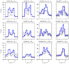 |
Fig. A.1. H2CO and CH3OH spectra, integrated over the central area of the dust trap using Keplerian masking (blue) and extracted from a rectangular box (grey). The grey shades indicate the noise levels in the spectra. The spectra are ordered by increasing Eu, following the values reported in Table 1. |
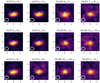 |
Fig. A.2. H2CO and CH3OH naturally weighted zero-moment maps using Keplerian masking. The plus symbol indicates the position of the star, and the beam is shown in the lower left of each map. |
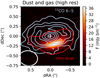 |
Fig. A.3. High-resolution image of the 13CO 6–5 zero-moment map (blue) and the 366 GHz continuum (red) at the original 0.18 × 0.14″ resolution. The contours of the 13CO show the 20%, 40%, 60%, and 80% of the peak, while the contours of the continuum indicate the 5σ level. This image demonstrates that the gas traces a full disk ring, whereas the millimetre dust grains are concentrated in the southern part of the disk. |
Appendix B: Rotational diagram analysis
This section contains more details on the analysis of the rotational diagram from Fig. B.1. Figure B.2 displays the corner plots, showing the posterior distributions and covariances of the fit that contains all line transitions, thus confirming that the fit has converged. The covariance is similar to previous studies of rotational diagrams of COMs in protoplanetary disks (e.g., Loomis et al. 2018).
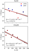 |
Fig. B.1. Rotational diagrams of H2CO and CH3OH using the integrated fluxes from this study and assuming optically thin emission. The integrated flux of the H2CO 91, 8 − 81, 7 transition from van der Marel et al. (2014) is included as a lower limit. The red line provides the best fit through the data points, and the grey lines are drawn from the posterior distribution from the fitting (Fig. B.2). |
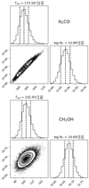 |
Fig. B.2. Posterior distributions of the column density and rotational temperature based on our optically thin line intensities of H2CO (left) and CH3OH (right). The best fit is shown in Fig. B.1. |
We estimated the ortho-to-para ratio of H2CO by fitting the ortho and para lines separately, without the ortho-to-para correction of three in the degeneracies used in Fig. B.1. The new rotational diagram with best fits and the posteriors are shown in Fig. B.3. The ortho lines have a best-fit Trot of 193 K and NT = 7.2 ± 0.7 × 1013 cm−2 and the para lines a Trot of 257
 K and NT = 5.9 ± 1.7 × 1013 cm−2. This implies an ortho-to-para ratio of 1.2 ± 0.4, which is well below the default value of 3. The lower value could indicate an ice formation rather than a gas formation route (e.g., Terwisscha van Scheltinga et al. 2021), which is consistent with our proposed scenario. However, if the optical depth of the ortho lines is underestimated (if the emitting area is smaller than assumed), this could also explain the lower value. Furthermore, for H2O it has been shown that the ortho-to-para ratio is reset after desorption from the ices (Hama et al. 2018); if the same is true for H2CO, the ortho-to-para ratio does not provide information about the formation origin. Regardless of the precise scenario, a low ortho-to-para ratio would imply a very cold formation location of only ∼10 K (Kahane et al. 1984), much lower than the current dust trap conditions.
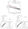 |
Fig. B.3. Rotational diagram of H2CO; similar to Fig. B.1, but without the default ortho-to-para correction of three for the para lines, with separate fits to the ortho and para lines. Bottom panels: posterior distributions of the best fits, as in Fig. B.2. |
Appendix C: Temperature structure
This section describes our analysis of the temperature structure and line ratios of IRS 48. We set up a series of physical-chemical models using DALI (Bruderer et al. 2012; Bruderer 2013) to compute the gas and dust temperature structure from the heating-cooling balance of gas and dust, following the parametrized model of the gas and dust surface density from van der Marel et al. (2016) that is consistent with the CO 6–5 isotopologue data presented in that work. The dust surface density was not explicitly fitted in that model, and with the gas-to-dust ratio of 20 used in that work the dust surface density at 60 au is Σd ∼ 0.005 g cm−2. As Ohashi et al. (2020) derived a much higher dust surface density of Σd ∼ 2–8 g cm−2, we explored the effect of the dust surface density on the radial and vertical temperature structure, using Σd ∼ 0.05, 0.5, and 5.0 g cm−2 between 60 and 80 au. Two sets of models were run: one with an increase in the large grains in the midplane with a larger degree of settling (settled models) and a second with an increase in all grains throughout the full dust column (full models). The vertical density structure in DALI was fixed to a Gaussian profile with different scale heights for the large and small grains to represent the settling, following Andrews et al. (2011):
![$$ \begin{aligned} \rho _{\rm l}&= \frac{\Sigma _{\rm l}}{\sqrt{2\pi }r\chi {h}} \exp \left[-\frac{1}{2}\left(\frac{\pi /2-\theta }{\chi {h}}\right)^2\right] ,\end{aligned} $$](/articles/aa/full_html/2021/07/aa41051-21/aa41051-21-eq5.gif)
![$$ \begin{aligned} \rho _{\rm s}&= \frac{\Sigma _{\rm s}}{\sqrt{2\pi }rh}\exp \left[-\frac{1}{2} \left(\frac{\pi /2-\theta }{h}\right)^2\right], \end{aligned} $$](/articles/aa/full_html/2021/07/aa41051-21/aa41051-21-eq6.gif)
where ρl and ρs are the dust density of large and small grains, respectively, h = hc(r/rc)ψ is the scale height, χ is the settling parameter, and θ is the vertical latitude coordinate measured from the pole. The large grain population contains dust grains from 0.005 μm to 1 mm, and the small grain population contains dust grains from 0.005 to 1 μm by convention. In the full disk model the settling degree χ is set to the default value of 0.2, while in the settled model χ is set to 0.1. The radial structure inside 60 au contains the inner dust disk (between rsub and rgap), the gas cavity rcavgas, and the dust cavity rcavdust, which are the same as in van der Marel et al. (2016), and we refer to that work for more details. All model parameter values are listed in Table C.1, and the results are shown in Figs. C.1 and C.2.
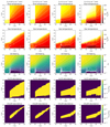 |
Fig. C.1. Temperature structure of the IRS 48 disk as computed by DALI, using the gas and dust density profile derived by van der Marel et al. (2016) for the settled models (dust density increase of the large grains in the midplane). The columns show the influence of the assumed dust surface density (or dust-to-gas ratio, as the gas surface density is set constant) on the UV field and gas temperature. The white contours in the temperature plots indicate steps of 20 K. |
 |
Fig. C.2. Temperature structure of the IRS 48 disk as computed by DALI, using the gas and dust density profile derived by van der Marel et al. (2016) for the full models (dust increase across the column). The columns show the influence of the assumed dust surface density (or dust-to-gas ratio, as the gas surface density is set constant) on the UV field and gas temperature. The white contours in the temperature plots indicate steps of 20 K. |
Model parameters of gas and dust surface density.
Next, we estimated the expected flux ratios for both optically thick and optically thin emission of the H2CO and CH3OH lines studied in this work. This was parametrized by setting an abundance of 10−7 and 10−9 (optically thick and thin, respectively) for both molecules in the regions in the disk where the extinction AV > 1 (shielding for photodissociation), radius r > 60 au (in the dust trap), and the dust temperature Tdust > Tsubl, with Tsubl = 66 K for H2CO and 100 K for CH3OH. These thresholds set the region where the molecule is expected to be in the gas phase. These regions are well above the regime where the majority of the large grains are located due to the settling. In the rest of the disk, these molecular abundances were set to 10−12. This leads to specific emitting layers in the disk where H2CO and CH3OH are located, which are used to ray-trace the lines to compute line ratios that can be compared with the data. The absolute fluxes are less relevant as the real molecular layers are likely much more complex. Additionally, as DALI is an axisymmetric model, the azimuthal structure is not constrained in this model.
The models show that the dust and gas temperature drop when the dust density is increased due to the stronger suppression of the UV field. This drop remains limited to the midplane when the dust density is only increased in that region, as opposed to an increase throughout the full column. This is illustrated directly in Fig. 3. The models show that the emitting layer shifts upwards in the disk for higher dust densities when the dust is distributed throughout the disk (‘full’) due to the sublimation temperature requirement. On the upper end, the emitting layer is constrained by the extinction requirement, which means that the layer becomes thinner in the high dust density models. In the most extreme case of Σd = 5 g cm−2, an additional emitting layer appears in the midplane as the dust becomes fully optically thick at the dust edge, leading to a strong vertical increase in temperature.
While the ray-traced line fluxes reproduce the H2CO fluxes reasonably well for the settled models for the 10−7 abundance, the CH3OH fluxes are at least a factor of ten too low. The models with 10−9 abundance and the full models with high dust density underestimate all fluxes by one to three orders of magnitude. The line ratios were derived and are compared with the line ratios in the RADEX plot in Fig. C.3. The line ratios for H2CO for 10−7 abundance are closer to the data values, suggesting that the H2CO emission is potentially optically thick (i.e., the emitting area is at least a factor of five smaller than our estimate). The ratios shift to slightly lower values for the higher dust density models, consistent with lower temperatures. For CH3OH the ratios are essentially the same for the two abundances and in a similar temperature regime as the data, suggesting that the emission remains optically thin for both. The ratios shift to higher values for the full models with high dust density, consistent with higher temperatures, which is the result of the strong upward shift in the emitting layers. However, the column density and flux drop significantly in that case, implying that this is not a realistic scenario. Overall, the spread in temperatures for the different ratios implies that the various lines trace different temperature regions in the disk, with potentially different abundances. A more detailed analysis is saved for future work.
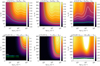 |
Fig. C.3. Expected line ratios as computed by RADEX for H2CO (top) and CH3OH (bottom) for a column density of 1014 cm−2. The white contours indicate the observed values and the dashed lines the uncertainty. The coloured lines indicate the ratios as computed for our DALI models of the settled model for fixed abundances of 10−7 and 10−9 in specific emitting layers, as described in the text. |
All Tables
All Figures
|
Fig. 1. Overview of the brightest H2CO and CH3OH lines using Briggs weighting, the 336 GHz continuum, and the 13CO 6–5 map, with a similar beam size for comparison. Top row: zero-moment maps, middle row: continuum and first-moment maps, and bottom row: disk-integrated spectra. The micron-sized grain distribution as traced by 19 μm VISIR data (Geers et al. 2007) is indicated in the continuum image. The source velocity is indicated by a vertical dotted line. The grey shades indicate the noise levels in the spectra. |
| In the text | |
|
Fig. 2. Radially and azimuthally averaged profiles of the brightest H2CO and CH3OH lines from the Briggs-weighted images, combined with the profiles from 13CO 6–5 and the 355 GHz continuum imaged at the same beam size of 0.55 × 0.44″. |
| In the text | |
|
Fig. 3. Temperature structure and proposed scenario for the release of the COMs in the dust trap. Top left: radial dust temperature profiles of the midplane. Top right: vertical gas temperature profiles at 65 au, just inside the dust trap. Both temperature profiles are based on our physical-chemical DALI models, with different dust surface densities (Figs. C.1 and C.2). In the midplane, the gas temperature is equal to the dust temperature. The plots demonstrate that the dust trap provides sufficiently low temperatures for a COM ice reservoir in the settled midplane, whereas the temperatures in the emitting layer are sufficiently high to explain the derived excitation temperatures. Bottom: sketch of the proposed scenario for the complex organic chemistry in a dust trap based on this work. The blue-orange gradient indicates the predicted temperature structure in the disk, the large arrows the vertical and radial transport of the icy pebbles, and the small arrow the thermal desorption at the inner edge of the dust trap. |
| In the text | |
|
Fig. A.1. H2CO and CH3OH spectra, integrated over the central area of the dust trap using Keplerian masking (blue) and extracted from a rectangular box (grey). The grey shades indicate the noise levels in the spectra. The spectra are ordered by increasing Eu, following the values reported in Table 1. |
| In the text | |
|
Fig. A.2. H2CO and CH3OH naturally weighted zero-moment maps using Keplerian masking. The plus symbol indicates the position of the star, and the beam is shown in the lower left of each map. |
| In the text | |
|
Fig. A.3. High-resolution image of the 13CO 6–5 zero-moment map (blue) and the 366 GHz continuum (red) at the original 0.18 × 0.14″ resolution. The contours of the 13CO show the 20%, 40%, 60%, and 80% of the peak, while the contours of the continuum indicate the 5σ level. This image demonstrates that the gas traces a full disk ring, whereas the millimetre dust grains are concentrated in the southern part of the disk. |
| In the text | |
|
Fig. B.1. Rotational diagrams of H2CO and CH3OH using the integrated fluxes from this study and assuming optically thin emission. The integrated flux of the H2CO 91, 8 − 81, 7 transition from van der Marel et al. (2014) is included as a lower limit. The red line provides the best fit through the data points, and the grey lines are drawn from the posterior distribution from the fitting (Fig. B.2). |
| In the text | |
|
Fig. B.2. Posterior distributions of the column density and rotational temperature based on our optically thin line intensities of H2CO (left) and CH3OH (right). The best fit is shown in Fig. B.1. |
| In the text | |
|
Fig. B.3. Rotational diagram of H2CO; similar to Fig. B.1, but without the default ortho-to-para correction of three for the para lines, with separate fits to the ortho and para lines. Bottom panels: posterior distributions of the best fits, as in Fig. B.2. |
| In the text | |
|
Fig. C.1. Temperature structure of the IRS 48 disk as computed by DALI, using the gas and dust density profile derived by van der Marel et al. (2016) for the settled models (dust density increase of the large grains in the midplane). The columns show the influence of the assumed dust surface density (or dust-to-gas ratio, as the gas surface density is set constant) on the UV field and gas temperature. The white contours in the temperature plots indicate steps of 20 K. |
| In the text | |
|
Fig. C.2. Temperature structure of the IRS 48 disk as computed by DALI, using the gas and dust density profile derived by van der Marel et al. (2016) for the full models (dust increase across the column). The columns show the influence of the assumed dust surface density (or dust-to-gas ratio, as the gas surface density is set constant) on the UV field and gas temperature. The white contours in the temperature plots indicate steps of 20 K. |
| In the text | |
|
Fig. C.3. Expected line ratios as computed by RADEX for H2CO (top) and CH3OH (bottom) for a column density of 1014 cm−2. The white contours indicate the observed values and the dashed lines the uncertainty. The coloured lines indicate the ratios as computed for our DALI models of the settled model for fixed abundances of 10−7 and 10−9 in specific emitting layers, as described in the text. |
| In the text | |
Current usage metrics show cumulative count of Article Views (full-text article views including HTML views, PDF and ePub downloads, according to the available data) and Abstracts Views on Vision4Press platform.
Data correspond to usage on the plateform after 2015. The current usage metrics is available 48-96 hours after online publication and is updated daily on week days.
Initial download of the metrics may take a while.