| Issue |
A&A
Volume 651, July 2021
|
|
|---|---|---|
| Article Number | A94 | |
| Number of page(s) | 12 | |
| Section | Interstellar and circumstellar matter | |
| DOI | https://doi.org/10.1051/0004-6361/202140655 | |
| Published online | 23 July 2021 | |
First survey of HCNH+ in high-mass star-forming cloud cores
1
INAF-Osservatorio Astrofisico di Arcetri,
Largo E. Fermi 5,
50125
Florence,
Italy
e-mail: This email address is being protected from spambots. You need JavaScript enabled to view it.
2
Centre for Astrochemical Studies, Max-Planck-Institute for Extraterrestrial Physics,
Giessenbachstrasse 1,
85748
Garching, Germany
3
Centro de Astrobiología (CSIC-INTA),
Ctra. de Ajalvir Km. 4,
Torrejón de Ardoz,
28850
Madrid, Spain
Received:
25
February
2021
Accepted:
14
May
2021
Abstract
Context. Most stars in the Galaxy, including the Sun, were born in high-mass star-forming regions. It is hence important to study the chemical processes in these regions to better understand the chemical heritage of the Solar System and most of the stellar systems in the Galaxy.
Aims. The molecular ion HCNH+ is thought to be a crucial species in ion-neutral astrochemical reactions, but so far it has been detected only in a handful of star-forming regions, and hence its chemistry is poorly known.
Methods. We observed with the IRAM 30 m Telescope 26 high-mass star-forming cores in different evolutionary stages in the J = 3−2 rotational transition of HCNH+.
Results. We report the detection of HCNH+ in 16 out of 26 targets. This represents the largest sample of sources detected in this molecular ion to date. The fractional abundances of HCNH+ with respect to H2, [HCNH+], are in the range 0.9−14 × 10−11, and the highest values are found towards cold starless cores, for which [HCNH+] is of the order of 10−10. The abundance ratios [HCNH+]/[HCN] and [HCNH+]/[HCO+] are both ≤0.01 for all objects except for four starless cores, which are well above this threshold. These sources have the lowest gas temperatures and average H2 volume density values in the sample. Based on this observational difference, we ran two chemical models, ‘cold’ and ‘warm’, which attempt to match the average physical properties of the cold(er) starless cores and the warm(er) targets as closely as possible. The reactions occurring in the latter case are investigated in this work for the first time. Our predictions indicate that in the warm model HCNH+ is mainly produced by reactions with HCN and HCO+, while in the cold model the main progenitor species of HCNH+ are HCN+ and HNC+.
Conclusions. The observational results indicate, and the model predictions confirm, that the chemistry of HCNH+ is different in cold–early and warm–evolved cores, and the abundance ratios [HCNH+]/[HCN] and [HCNH+]/[HCO+] can be useful astrochemical tools to discriminate between different evolutionary phases in the process of star formation.
Key words: ISM: molecules / stars: formation / radio lines: ISM / ISM: clouds
© ESO 2021
1 Introduction
It is now clear that the Sun and most stars in the Milky Way are born in rich clusters that include or are close to high-mass stars (e.g. Carpenter 2000; Pudritz 2002; Adams 2010; Rivilla et al. 2014; Lichtenberg et al. 2019). Therefore, the study of the chemical content and evolution of high-mass star-forming regions can give us important information about the chemical heritage of the Solar System and of most stars in the Milky Way. Despite the importance of studying the chemistry of high-mass star-forming cloud cores (i.e. compact structures with mass ~ 10−100 M⊙ that have the potential to form single high-mass stars and/or clusters), an evolutionary classification is not yet clear, due to both observational and theoretical problems (e.g. Beuther et al. 2007; Tan et al. 2014; Motte et al. 2018; Padoan et al. 2020).
Several attempts to empirically give an evolutionary classification of high-mass star-forming cores have been proposed, which can all be tentatively summarised in three coarse phases: (1) high-mass starless cores (HMSCs), which are dense infrared-dark cores characterised by low temperatures (~ 10−20 K) and high densities (n ≥ 104−105 cm−3), and without clear signs of ongoing star formation like strong protostellar outflows and masers; (2) high-mass protostellar objects (HMPOs), which are collapsing cores with evidence of one (or more) deeply embedded protostar(s), typically characterised by higher densities and temperatures (n ≃ 106 cm−3, T ≥20 K); (3) ultra-compact H II regions (UCHIIs), which are zero age main sequence stars associated with an expanding H II region whose surrounding molecular cocoon (n ≥ 105 cm−3, T ~20−100 K) is affected physically and chemically by its progressive expansion.
Regardless of the evolutionary stage, high-mass star-forming cores are characterised by a complex and rich chemistry (e.g. Fontani et al. 2007; Bisschop et al. 2007; Foster et al. 2011; Belloche et al. 2013; Vasyunina et al. 2014; Coletta et al. 2020). The new generation telescopes have provided a growing amount of observational results including, thanks to their high sensitivity, the detection of rare species (i.e. species with fractional abundance with respect to H2 lower than ~10−10). These species can have important implications not only for our understanding of the still mysterious process of high-mass star formation, but also for the chemistry that the primordial Solar System might have inherited from its birth environment (e.g. Beltrán et al. 2009; Fontani et al. 2017; Ligterink et al. 2020; Rivilla et al. 2020; Mininni et al. 2020). Among these rare species, protonated hydrogen cyanide, HCNH+ (or iminomethylium), is important in astrochemistry because it is thought to be the main precursor of HCN and HNC. They are both among the most abundant species in star-forming regions, and are believed to have a high pre-biotic potential (Todd & Öberg 2020). Despite its importance, and after the first discovery towards SgrB2 (Ziurys & Turner 1986), HCNH+ has been detected in a handful of other star-forming regions: the TMC-1 dark cloud, the DR21(OH) H II region (Schilke et al. 1991), and the low-mass pre-stellar core L1544 (Quénard et al. 2017).
In this work we report 16 new detections of HCNH+ towards 26 high-mass star-forming cores almost equally divided into HMSCs, HMPOs, and UCHIIs. In Sect. 2 we describe the sample and the observational dataset; in Sect. 3 we present the observational results, which we discuss in Sect. 4; in Sect. 5 we describe the chemical model we used to interpret the observational results; and in Sect. 6 we summarise our main findings.
2 Sample and observations
The 26 targets we observed are listed in Table 1. They were taken from the sample presented first by Fontani et al. (2011) and divided into the three gross evolutionary categories discussed in Sect. 1: 10 HMSCs, 9 HMPOs, and 7 UC HIIs (see Fontani et al. 2011 for details on the source selection criteria). The spectra analysed in this work are part of the dataset published in Fontani et al. (2015a) obtained with the IRAM 30m telescope. In particular, the analysed transition, HCNH+ J = 3−2, was detected in the band at 1.2 mm of that dataset covering frequencies in the range 216.0–223.78 GHz. The spectra were observed with a telescope beam of ~ 11′′, and a spectral resolution of ~ 0.26 km s−1. Details of the observations (weather conditions, observing technique, calibration, pointing, and focus checks) are given in Fontani et al. (2015a). The analysed line has a rest frequency of ~ 222 329.277 MHz, energy of the upper level Eu ~ 21.3 K, Einstein coefficient Aij = 4.61 × 10⁻⁶ s−1, and degeneracy of the rotational upper level gu = 7. All these spectral parameters are from the Cologne Database for Molecular Spectroscopy (CDMS; Endres et al. 2016). The spectroscopy was determined by Araki et al. (1998); the dipole moment is from Botschwina (1986). According to the collisional coefficients given in Nkem et al. (2014), which are ~ 1−1.5 × 10⁻¹⁰ s−1 in the temperature range 10–100 K, the critical density of the transition is ~ 4 × 104 cm−3. The lines were fitted with the CLASS package of the GILDAS1 software using standard procedures.
3 Results
3.1 Detection rate and line shapes
We detected HCNH+ J = 3−2 with a signal-to-noise ratio (S/N) higher than ~3 towards 14 out of the 26 targets. In two cases, I20293–WC and 23 033+5951, the peak main beam temperature is slightly below the 3σ rms, but the line profile suggests a real line at the limit of the detection level. Hence, we consider them as tentative detections, which provides a total of 16 detected sources including the tentative ones (detection rate ~ 62%). The transition has hyperfine structure, however, that cannot be resolved in our spectra because the separation in velocity of the components is smaller than the velocity resolution. Therefore, we fitted the lines with single Gaussian profiles. This method gives good results with residuals lower than, or comparable to, the noise in the spectra.
Table 1 reports the results of the Gaussian fits to the lines: integrated line intensity (∫ TMBdV), velocity at line peak (Vp), line full width at half maximum (FWHM), peak main beam temperature ( ), and 1σ rms in the spectrum (1σ). The uncertainties on Vp and on FWHM are given by the fit procedure. The uncertainties on ∫ TMBdV are the sum in quadrature of the error given by the fit and the calibration error on TMB (assumed to be 10%). The latter is dominant in the sum in quadrature.
The spectra and their fits are shown in Fig. 1. In two sources, 18 089–1732 and G5.89–0.39, the line profile cannot be fitted with a single Gaussian. Both spectra show an excess emission in the red tail of the line (see Fig. 1). Towards G5.89–0.39 this excess has the form of a high-velocity wing. Hence, it likely arises from the red-shifted lobe of the outflow associated with the embedded UC HII region (Zapata et al. 2020). Towards 18 089–1732 the excess emission has the shape of a Gaussian peak with intensity almost half of the main peak. Hence, in this case it is more likely due either to a secondary velocity feature or to another line blended with the HCNH+ J =3−2 line. High excitation lines (Eu ~ 200 K) of CH3OCH3 detected in this source (Coletta et al. 2020) are predicted at ~ 222 326 MHz, which could hence contribute to the secondary peak centred approximately at ~ 222 327 MHz. Moreover, the profile of the H13 CO+ J = 1−0 does not show this secondary peak (Fig. 2), and hence a second velocity feature is very unlikely. A contribution from the red lobe of the outflow associated with the embedded hyper-compact HII region is also possible (Beuther et al. 2010), but because it is not seen in H13 CO+ J = 1−0, its contributionto this secondary peak should be negligible. In general the lack of high-velocity wings, except maybe in the two cases discussed above, indicates that the emission of the line does not arise from shocks and/or outflows, but likely from more quiescent material.
Because HCNH+ was detected in a handful of star-forming regions before this study, it is not yet clear what kind of material (i.e. with what physical and kinematical properties) is responsible for the emission of this molecule. To investigate this, in Fig. 2 we compare the profiles of HCNH+ J = 3−2 with those of H13 CO+ J = 1−0 analysed in Fontani et al. (2018), thought to be a good tracer of the envelope of star-forming cores. Inspection of the plot suggests that in some sources (e.g. G028–C1, AFGL5142–EC, 05358–mm1, I20293–MM1, 19 410+2336) the two lines have similar peak velocity, suggesting a common origin in the envelope of the cores. On the other hand, in some targets (e.g. G034–F1, I20293–WC, I22134–VLA1, and G5.89-0.39) the HCNH+ emission does not coincide with the central velocity of H13 CO+, even though towards G034–F1 and I20293–WC, the H13 CO+ J = 1−0 shows multiple velocity features, and the HCNH+ J = 3−2 emission is centred on one of these. These second velocity features, in principle, could also be originated by self-absorption or polluting lines from other species. These scenarios, however, are both unlikely in G034–F1 and I20293–WC, because self-absorption signatures were never observed in other lines towards these sources, and polluting lines are very unlikely in cold HMSCs (like these two targets). Furthermore, a second velocity feature towards G034–F1 was found in the HCN isotopologues by Colzi et al. (2018a).
The stronger H13 CO+ lines generally have broader line widths than the HCNH+ lines, except for a few targets (G034–G2, 18 089–1732, I22134–VLA1). In addition, we see no hints of high-velocity wings in HCNH+ J = 3−2, except for the already discussed spectrum of G5.89–0.39. However, high-velocity wings could not be detected due to the limited S/N in the spectra. All this indicates that the gas emitting HCNH+ is mostly quiescent, or not clearly associated with shocks, and that there is not a general agreement with the profiles of the H13 CO+ J = 1−0 lines. We propose, in the targets where both lines have the same velocity peak, that the HCNH+ J = 3−2 line arises from the envelope of the cores, but likely from a more compact portion than that traced by H13 CO+ J = 1−0, because the HCNH+ J = 3−2 line has a higher energy of the upper level than H13 CO+ J = 1−0 (21.3 K versus 4 K), and the spectra were observed with different beam sizes (~ 11′′ versus ~ 28′′).
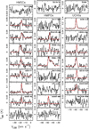 |
Fig. 1 Observed spectra of HCNH+ J = 3− 2 obtained with the IRAM 30 m telescope. For each spectrum the velocity interval shown on the x-axis is ± 20 km s−1 around the systemicvelocity listed in Table A.1 of Fontani et al. (2011). The red curves represent Gaussian fits to the detected lines. For 18 089–1752 a two-Gaussian fit was performed. |
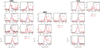 |
Fig. 2 Comparison among the observed profiles of H13CO+ J = 1− 0 (black histograms) and HCNH+ J = 3−2 (red histograms) towards, from left to right, the HMSCs, the HMPOs, and the UCHIIs detected in HCNH+ (Table 1). The red number in each plot indicates the multiplicative factor applied to the HCNH+ spectrum. The blue dashed vertical line indicates the systemic velocity used to centre the observed spectra (see e.g. Fontani et al. 2015a). The peak velocities of HCNH+ are listed in Table 1. |
3.2 Total column densities and abundances of HCNH+
Assuming that the lines are optically thin and in Local Thermodynamic Equilibrium (LTE), from ∫ TMBdV, we computed the beam-averaged total columndensities of HCNH+, Ntot (HCNH+), using Eq. (1) of Fontani et al. (2018). For undetected sources, we estimated the upper limits on Ntot (HCNH+) from the upper limit on the integrated intensity. This was computed from the relation 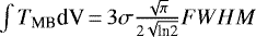 , which expresses the integral in velocity of a Gaussian line with peak intensity given by the 3σ rms in the spectrum. We assumedas FWHM the average value obtained from the detected lines in each evolutionary group which the undetected source belongs to: 2.5 km s−1 for HMSCs, 1.6 km s−1 for HMPOs, and 2.4 km s−1 for UCHIIs (seeTable 1).
The assumption of optically thin emission is consistent with the low abundance of the molecule and with the fact that the observed line shapes generally have no hints of high optical depths, such as asymmetric or flat-top profiles. Only towards G034–G2 could the almost flat-top line shape indicate non-negligible optical depths. Hence, in this source the HCNH+ total column density should be regarded as a lower limit. The assumption of LTE is also reasonable because the critical density of the line (~ 4 × 104 cm−3; see Sect. 2) is smaller than, or comparable to, the average H2 volume densities of the sources. These values, calculated within a beam of 28′′, are between 104 and 106 cm−3 (see e.g. Fontani et al. 2018 and Sect. 4). A few sources have H2 volume density values of ~ 1−2 × 104 cm−3: the HMSCs G034–F2, G034–F1, and G028–C1, and the UCHII I22134–VLA1 (see Sect. 4). For these targets, the approximation might not be valid. We estimated by how much Ntot (HCNH+) would change in the conservative case where the excitation temperature is lower than the kinetic temperature by 10 K: Ntot (HCNH+) would increase by a factor ~4. Therefore, in the following the column densities of these targets should be considered lower limits.
The total column densities, averaged within the telescope beam of 11′′, are in the range 0.5−10 × 1013cm−2. If we analyse the three evolutionary groups separately, we find hints of possible differences. The average values are ~ 1.5 × 1013cm−2 for the HMSCs, ~ 1.25 × 1013cm−2 for the HMPOs, and ~ 2.7 × 1013cm−2 for the UCHIIs. However, the average value in the UCHIIs is strongly biased by G5.89–0.39, which is by far the most luminous object in the sample. Without G5.89–0.39 the average value in the UCHIIs is ~ 1.3 × 1013cm−2, consistent with those of the other two evolutionary groups.
We computed abundances of HCNH+ relative to H2 by using the H2 column densities published in Fontani et al. (2018). These were average values derived in an angular diameter of 28′′, hence the HCNH+ column densities were smoothed to this larger angular diameter. The corresponding abundances, [HCNH+], are listed in Table 1, and range from ~0.9 to ~14 × 10−11. Interestingly, HMPOs and UCHIIs have average [HCNH+] of the order of 10−11 and are consistent with each other (specifically, ~2.5 and ~3.7 × 10⁻¹¹, respectively), while HMCSs have an average [HCNH+] of ~ 7.3 × 10⁻¹¹ (i.e. a factor 2–3 higher). In particular, the HMSCs with the highest abundances are all classified as cold or quiescent by Fontani et al. (2011), and have [HCNH+] of the order of × 10−10.
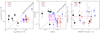 |
Fig. 3 Left panel: comparison between Ntot (HCNH+) and Ntot (HCN). The latter was derived from the H13CN J = 1− 0 line (Colzi et al. 2018b), assuming the same Tex, by correcting it for the 12C/13C ratio obtained at the Galactocentric distance of the sources from the trend of Yan et al. (2019). Ntot (HCNH+) has been rescaled to the (larger) beam of the H13CN observations, ~ 28′′. Red stars are HMPOs; blue stars are UCHIIs; black symbols are HMSCs (filled circles for quiescent,stars for warm; see Table 1). Triangles indicate upper limits on Ntot (HCNH+). The dashed line is the locus where Ntot (HCNH+) = 0.01 Ntot (HCN). Middle panel: same as left panel, but for the fractional abundances with respect to H2 calculated on a beam of ~28′′. The purple rectangle indicates the range of abundances that reproduces the observed [HCN], and [HCNH+] in the predictions of the WM (see Sect. 5 and right panel of Fig. 7). Similarly, the cyan square indicates the prediction of the CM (see Sect. 5 and left panel of Fig. 7). Right panel: comparison between the line FWHM of HCNH+, derived in this work from the J = 3−2 line, and H13 CN, derived by Colzi et al. (2018a) from the J = 1−0 line at ~87 GHz. The symbols have the same meaning as those in the left and middle panels. |
4 Discussion of the observational results
One of the most important and direct findings from the parameters in Table 1 is that the HMSCs classified as quiescent have HCNH+ abundances that are about an order of magnitude higher with respect to warm(er) and/or more evolved objects. This suggests that in cold and quiescent cores some formation pathways of HCNH+ are more efficient than in warmer cores and/or that some destruction pathways are less efficient. The chemistry of HCNH+ is thought to be related to that of HCN, HCO+, and CN, as discussed in Quénard et al. (2017). However, Quénard et al. (2017) focussed on the pre-stellar core L1544 (i.e. a cold core with a known physical structure). It is not yet clear what the dominant formation pathways are in warmer environments (and under different physical conditions in general).
To investigate the chemical origin of HCNH+ we searched for correlations between some physical parameters of HCNH+ and those of HCN, HCO+, and CN. In Fig. 3 we compare column densities, abundances, and FWHM of HCNH+ and HCN. Figure 4 shows the same comparison between HCNH+ and HCO+. We note that the column densities of HCN and HCO+ were calculated from the data of H13CN and H13 CO+ published inColzi et al. (2018a) and Fontani et al. (2018), respectively. The column densities of both H13 CN and H13 CO+ were computed assuming the Tex in Table 1, and converted to those of the main isotopologues using the 12 C/13C ratio at the Galactocentric distance of the sources. This latter value was derived from the most recent trend of Yan et al. (2019). Calculated 12 C/13C ratios are in the range ~40−70. The uncertainties on these ratios, calculated propagating the errors on the parameters of the Galactocentric trend, are of the order of 30%. As for HCNH+, the final Ntot (HCN) and Ntot (HCO+) were scaled to the same beam of ~28′′, and the abundances [HCN] and [HCO+] were computed dividing Ntot (HCN) and Ntot (HCO+) by the same Ntot (H2) used for HCNH+.
Two relevant results emerge clearly from the plots in Figs. 3 and 4: first, the abundance ratios [HCNH+]/[HCN] and [HCNH+]/[HCO+] are both ≤0.01 for all objects except for the four quiescent HMSCs G034–G2, G034–F2, G034–F1, and G028–C1, for which they are one order of magnitude above this threshold. This difference could be even more pronounced for three of these four sources because, as discussed in Sect. 3.2, [HCNH+] might be underestimated because the transition could be sub-thermally excited. Second, the FWHM of the lines of the different species do not appear to be clearly correlated. However, if the four quiescent HMSCs mentioned above are excluded, a tentative correlation is apparent in Figs. 3 and 4, with Spearman ρ correlation coefficients ~0.55 and ~0.63, respectively.
These findings suggest that the dominant formation pathways of HCNH+ in cold and warm regions are likely different. Only one quiescent HMSC, I20293–WC, does not follow this different behaviour. However, the detection of HCNH+ is tentative towards this source (see Table 1), and the core, even though considered quiescent based on its low kinetic temperature (Fontani et al. 2011), is embedded in a star-forming region harbouring a more evolved object (e.g. core I20293–MM1, included in the HMPOs). Therefore, the chemistry in this target could be influenced by the complex environment in which it is embedded.
Figure 5 shows the same comparison of physical parameters as in Figs. 3 and 4 for CN. The properties of this species were derived from 13 CN by Fontani et al. (2015b). Figure 5 shows a less clear dichotomy between HMSCs and the more evolved targets, but unfortunately the comparison is affected by the non-detection of 13 CN in all the quiescent HMSCs. However, also in this case the [HCNH+]/[CN] ratio in warm and/or evolved objects is ≤0.01. The FWHM of the lines does not seem correlated either, and hence the possible chemical relation between HCNH+ and CN seems unlikely.
Finally,in Fig. 6 we plot the column density ratio Ntot (HCNH+)/Ntot (HCN) as a function of the following core physical parameters: Ntot (HCN); volume density of H2, n(H2); gas kinetic temperature, Tk, taken fromFontani et al. (2011) and used in Colzi et al. (2018a) to compute the HCN column densities; dust temperature, Tdust, calculated by Mininni et al. (2021) from grey-body fits to the spectral energy distribution of the sources derived from the Herschel bands. n(H2) is an averagevalue within 28′′ computed from the column density of H2 given in Fontani et al. (2018) assuming spherical sources for simplicity. Based on this plot, the different behaviour of cold and warm sources is very clear: colder and less dense objects have Ntot (HCNH+)/Ntot (HCN) ratios that are about an order of magnitude higher than warmer and denser ones.
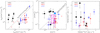 |
Fig. 4 Left panel: comparison between Ntot (HCNH+) and Ntot (HCO+). The latter was computed from Ntot (H13 CO+) taken from Fontani et al. (2018) by correcting it for the 12C/13C ratio obtained at the Galactocentric distance of the sources from the trend of Yan et al. (2019). Middle panel: same as left panel, but for the abundances relative to H2. As in the middle panel of Fig. 3, the purple rectangle and the cyan square show the predictions of the WM and CM (Sect. 5 and Fig. 7), respectively, that best reproduce the observed abundances of the three species HCNH+, HCN, and HCO+. Right panel: comparison between the line FWHM of HCNH+, derived in this work from the J = 3−2 line, and H13CO+, derived in Fontani et al. (2018) from the J = 1−0 line at ~87 GHz. The symbols have the same meaning as those in the left and middle panels. |
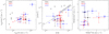 |
Fig. 5 Same as Fig. 3, but for the comparison between HCNH+ and CN. For CN, Ntot (left panel), [CN] (middle panel), and FWHM (right panel) are derived from observations of the 13 CN N = 2− 1 line at ~217 GHz, published in Fontani et al. (2015b). Ntot (HCNH+) and Ntot (CN) are averaged within the same beam of ~11′′, and left-pointing triangles are upper limits on Ntot (CN), while down-pointing triangles are upper limits on Ntot (HCNH+). [HCNH+] and [CN] areaveraged within a beam of 28′′. |
5 Chemical modelling
In this section we investigate the main routes of formation and destruction of HCNH+ and HCN, together with the possible chemical relation with HCO+, for two different chemical models that represent the colder and warmer conditions of the sample of high-mass star-forming regions studied in this work.
5.1 Description of the models
For the chemical simulations we use our gas-grain chemical code, recently described in Sipilä et al. (2019a,b). The chemical networks used here contain deuterium and spin-state chemistry (see Sipilä et al. 2019b, and references therein). While we do not explicitly consider deuterium chemistry in this paper, the inclusion of spin-state chemistry is important due to its effect on nitrogen chemistry (e.g. Dislaire et al. 2012). The chemical network contains a combined total of 881 species and 40 515 reactions (37 993 gas-phase reactions and 2519 grain-surface reactions). We have excluded all molecules that contain more than five atoms so that the chemical simulations can run faster; this is justified in the present context where we study the chemistry of molecules with four atoms or fewer. The initial abundances adopted in the models are summarised in Table 2.
To discuss the results obtained from the observations we decided to model two types of molecular clouds defined dividing the sample of sources into two sub-groups:
-
cold model (CM): defined from the four sources with a Tdust of about 10 K (see right panel of Fig. 6). These sources are the HMSCs G034–G2, G034–F1, G034–F2, and G028–C1;
-
warm model (WM): defined from all of the other sources, which have Tdust > 10 K.
We fixed the cosmic-ray ionisation rate (ζ), the visual extinction (AV), the grain albedo (ω), the grain radius (ag), the grain material density (ρg), the ratio of the diffusion to the binding energy of a species on dust grains (ϵ), and the dust-to-gas mass ratio (Rg) to the values given in Table 3. The gas temperature (Tgas) and total number density of H nuclei2 (nH) of the two models were defined respectively from the average Tdust and n(H2) of the two sub-groups of sources. We decided to use the dust temperatures instead of the kinetic temperatures because they were all derived with the same method (Mininni et al. 2021), while the kinetic temperatures were not; we assumed Tgas = Tdust for simplicity. For the cold model Tgas = 10 K and nH = 3.4 × 104 cm−3, and for the warm model Tgas = 27 K and nH = 2.4 × 105 cm−3. We adopted as initial conditions those used by Colzi et al. (2020) with an ortho-para ratio (o/p) of 10−3. Since in warm regions (>20 K) the o/p could be higher, and because N chemistry may be affected by it, we tried also to assume an o/p for the WM of 10−2 and of 10−1. This test was done with a fixed temperature of 27 K and we do not take into account the possibility that the o/p could be even higher while the temperature increases. In both cases the results that are discussed in the next section do not change.
It should be noted that for this work, both for the observations and for the chemical modelling, we discard any possible effect from the chemical isotopic fractionation of carbon, which could modify the observed and modelled abundances of HCN and HCO+ at most by a factor of three (see Colzi et al. 2020). Gas-grain chemistry is followed in our chemical models, and is important in the differentiation between the warm and cold sources, as in the former CO can be mainly maintained in the gas phase (27 K is just above the sublimation temperature of CO), thus contributing to the higher HCO+ abundances in warm regions.
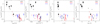 |
Fig. 6 Comparison between the column density ratio Ntot (HCNH+)/Ntot(HCN) and the following physical parameters of the cores (from left to right): Ntot (HCN), n(H2), Tk, and Tdust. The dashed line in each plot indicates Ntot (HCNH+)/Ntot(HCN) = 0.01. |
Initial abundances with respect to nH (adapted from Semenov et al. 2010).
Values of the physical parameters fixed in each model.
5.2 Model predictions
Figure 7 shows the predicted abundances for HCNH+, HCN, and HCO+. These predictions are plotted together with the range of the observed abundances, derived as explained in Sect. 3.2. For the CM the three abundances can be partially reproduced at about tCM = 4 × 10⁵ yr. For theWM this happens at two times, 5 × 10⁴ yr and 3 × 10⁶ yr, but for this discussion we decided to take into account only the earlier one (tWM = 5 × 10⁴ yr), which ismore representative of the life-time of massive star-forming regions (e.g. Motte et al. 2018). Moreover, at these times the abundance of HCN is equal to that of HCO+ as it is observed towards the sources studied in this work (see Figs. 3 and 4).
On these timescales most of the HCN and HCNH+ are already formed through the early-time chemistry (see e.g. Hily-Blant et al. 2010), HCN being mainly formed from
 (1)
(1)
and HCNH+ from
 (2)
(2)
The abundances of both HCN and HCNH+ increase by one order of magnitude at chemical times of 104 yr (Fig. 7).
As shown in Fig. 8, the observed HCNH+/HCN ratio cannot be reproduced by our chemical models on the timescales for which the abundances are reproduced. The predicted HCNH+/HCN ratio at tCM is ~ 0.02, lower than the observed ratios, and at tWM is ~ 0.01, slightly higher than what is observed. However, observations and model predictions agree with a higher HCNH+/HCN ratio in colder sources with respect to the warmer ones.
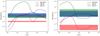 |
Fig. 7 Time evolution of HCNH+, HCN, and HCO+ abundances with respect to H2 for the CM (left panel) and for the WM (right panel). The coloured horizontal bands represent the ranges of observed abundances for HCNH+ (red), HCN (green), and HCO+ (blue), for the two sub-groups of sources. |
5.3 Formation and destruction reactions of HCNH+
To perform a detailed analysis and discuss the observed differences between the two sub-groups of sources (i.e. cold early starless cores and warmer evolved objects), we studied in detail the main reactions of formation and destruction that involve HCN, HCNH+, and related chemical species. In particular, we took into account the tCM and tWM times. In both models HCO+ is formed mainly from CO + H and mainly destroyed by HCO+ dissociative recombination. However, as we discuss later, its presence is very important in the cycle of reactions involved in the warm model.
Regarding the cold model, HCNH+ is mainly formed via
 (3)
(3)
 (4)
(4)
and
 (5)
(5)
and mainly destroyed by dissociative recombination forming HCN, HNC, and CN with almost the same probability (33.5, 33.5, and 33%, respectively; Semaniak et al. 2001):
 (6)
(6)
 (7)
(7)
and
 (8)
(8)
Moreover, HCN+ is mainly formed via CN + H closing this part of the cycle of reactions (Woon & Herbst 2009). Another cycle of reactions involves HCN, which at tCM is mainly formed via reaction (6) and mainly destroyed by the presence of HCO+, C+, and H
 . All of this is in agreement with the predictions of Hily-Blant et al. (2010) and Loison et al. (2014) for low-temperature pre-stellar cores and dark molecular clouds, respectively. More recently, for HCNH+, this was also confirmed by Quénard et al. (2017) towards the pre-stellar core L1544.
The novelty of this work is the study of the main chemical reactions for these chemical species in an environment that is warmer and denser than in the previous studies. From the WM we find that HCNH+ is mainly formed via
 (9)
(9)
instead of reactions (3) and (4). Although these two reactions still occur, they are not efficient any more for the formation of protonated HCN because the abundances of HCN+ and HNC+ decrease by three orders of magnitude with respect to the CM. The cycle of main reactions for the warm model is shown in Fig. 9. These chemical pathways are in agreement with the tentative correlations found for the FWHM between HCNH+ and HCN and HCO+.
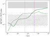 |
Fig. 8 Predicted HCNH+/HCN ratio for the CM (green solid line) and for the WM (dashed green line). The grey shaded areas represent the range of observed HCNH+/HCN ratios for the CM (filled area), and for the WM (striped area). The purple vertical lines indicate the times at which the abundances of HCNH+, HCN, and HCO+ are reproduced by the CM (tCM = 4 × 10⁵ yr, solid line), and by the WM (tWM = 5 × 10⁴ yr, dashed line). |
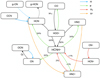 |
Fig. 9 Scheme of the chemical network that connects the main molecular species investigated in this work for the WM (see Sect. 5.1). The prefix g- indicates molecules in icy mantles on dust grains. The arrows are colour-coded depending on the involved reactant: H (blue), H2 (red), free electrons (green), H+ (orange), other species (black; the reactant is indicated on the side). Dashed arrows refer to transitions from solid to gas phase, or vice versa. For the reactions forming and destroying HCNH+, their relative contribution (in percentage) is also indicated. |
5.4 Discussion of the assumed parameters
It is worth noting that the sources have very complex structure, with dense cores embedded in a diffuse envelope, and also with the possible presence of extended outflows from the massive protostellar objects. In these models we simplify the physical geometry of the sources, and most of the parameters are assumed to be constant during the chemical evolution, possibly affecting the predicted abundances. Hence, we checked whether changing some of the physical parameters of the two models could lead to a better agreement with the absolute HCNH+/HCN ratios observed.
First of all, we tested higher values of the cosmic-ray ionisation rate with respect to the canonical value of 1.3 × 10⁻¹⁷ s−1 (e.g. Padovani et al. 2009), of 10−16, 10−15, and 10−14 s−1 (e.g. López-Sepulcre et al. 2013; Fontani et al. 2017). We find a higher HCNH+/HCN ratio (up to 0.04 already at 105 yr) at the lower edge of the observed values, for higher ζ in the CM (see left panel of Fig. 10). The presence of more ions favours the destruction of HCN over the formation of HCNH+. Moreover, this trend is the same for the WM, making the observed values reproduced for lower ζ (see right panel of Fig. 10). However, these trends are hard to understand because the ζ measured towards HMSCs are lower with respect to those found towards protostellar objects (e.g. Fontani et al. 2017). Another discrepancy is that the observed abundances of the molecules could not be reproduced, for both models, at times when the HCNH+/HCN ratio matches (see Figs. A.1–A.3). Thus, the cosmic-ray ionisation rate could not help us to explain the observed values.
Secondly, we investigated the possibility of a higher number density of hydrogen nuclei for the CM. In fact, nH were found from the H2 column densities, which in turn were derived in an area with angular dimension 28′′. However, the emission is not resolved and in principle it could mainly come from a smaller region (dense cores inside the high-mass clump). This would lead to higher nH. Assuming a density of one order of magnitude higher (nH = 3.4 × 105 cm−3) we find a better agreement with respect to the observed abundances of HCN, which are lower with respect to the predictions of the initial cold model (Fig. 11). The higher density, together with the low temperature, makes adsorption onto grain surfaces more efficient. However, the abundance of HCNH+ also decreases.
Finally, since high-mass protostellar objects are born in a gas that was previously a starless core, we tried to model the warm sources using as initial conditions the abundances of the CM at 4 × 10⁵ yr, the time in which the CM observations are reproduced. Interestingly, we found a warm model with almost constant abundances for the three models, well reproduced by the observations of HCN and HCO+, while slightly above with respect to the observed HCNH+ (Fig. 12). This leads to the same result obtained in the original WM, but spread during the chemical evolution.
In conclusion, we have found that a change in the initial conditions or in some of the initial parameters of the chemical model would not lead to the absolute observed HCNH+/HCN ratios. Many of the relevant reactions in the chemical model are not well constrained, and perhaps some important pathways are missing. For example, reactions (3), (4), and (9) in the KInetic Database for Astrochemistry (KIDA) network are just estimated and laboratory measurements are needed to obtain the correct molecular abundances.
6 Summary and conclusions
We have presented the first survey of HCNH+ J = 3−2 lines, observed with the IRAM 30 m telescope, towards 26 high-mass star-forming regions. We report 14 detections and 2 tentative detections, for a total detection rate of ~62%. The total column densities, Ntot (HCNH+), calculated assuming optically thin lines and local thermodynamic equilibrium conditions, are in the range 0.5−10 × 1014 cm−2. The abundances of HCNH+ with respect to H2 are in the range 0.9−14 × 10−11, and the highest values are found towards the coldest HMSCs, for which [HCNH+] is of the order of 10−10. The abundance ratios [HCNH+]/[HCN] and [HCNH+]/[HCO+] are both ≤0.01 in all targets except towards the four coldest HMSCs. Hence, the dominant formation pathways of HCNH+ in cold–early and warm–evolved regions are likely different. We have run two chemical models, one cold and one warm, in an attempt to reproduce our results. Besides the different temperatures, the two models are also adapted to match as closely as possible the average physical conditions of the four cold(est) HMSCs and the other sources. In particular, the main chemical reactions leading to the formation and destruction of HCNH+ in the warm model are investigated in this work for the first time. Our predictions indicate that HCO+ and HCN/HNC are indeed the dominant progenitor species of HCNH+ in the warm model, while in the cold model HCNH+ is mainly formed by HCN+ and HNC+. Another important result of this study is that the abundance ratios [HCNH+]/[HCN] and [HCNH+]/[HCO+] can be a useful astrochemical tool for discriminating between different evolutionary phases in the process of star formation. Naturally, higher angular resolution observations will allow us to better constrain the precise location and the extent of the emitting region of HCNH+ in the sources. More transitions will also help in constraining more precisely the excitation conditions, both crucial elements to better define the range of physical parameters appropriate to model the chemistry.
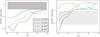 |
Fig. 10 Predicted HCNH+/HCN ratio for the CM (left panel) and the WM (right panel), assuming different cosmic-ray ionisation rates, ζ. The grey shaded areas represent the range of observed HCNH+/HCN ratios for the CM (filled area in the left panel), and for the WM (striped area in the right panel). |
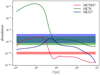 |
Fig. 11 Time evolution of HCNH+, HCN, and HCO+ abundances with respect to H2 for the cold model, but assuming a higher nH of 3.4 × 105 cm−3. The coloured horizontal areas are the same as in the left panel of Fig. 7. |
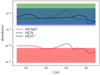 |
Fig. 12 Time evolution of HCNH+, HCN, and HCO+ abundances with respect to H2 for the warm model, found assuming as initial conditions the abundances of the CM at tCM. The coloured horizontal areas are the same as the right panel of Fig. 7. |
Acknowledgements
We thank the anonymous referee for their valuable and constructive comments. F.F. is grateful to the IRAM 30m staff for their precious help during the observations. L.C. acknowledges financial support through Spanish grant ESP2017-86582-C4-1-R (MINECO/AEI). L.C. also acknowledges support from the Comunidad de Madrid through the Atracción de Talento Investigador Modalidad 1 (Doctores con experiencia) Grant (COOL: Cosmic Origins Of Life; 2019-T1/TIC-15379; PI: Rivilla). The research leading to these results has received funding from the European Commission Seventh Framework Programme (FP/2007-2013) under grant agreement No 283393 (RadioNet3).
Appendix A Model predictions for different ζ
We show in this appendix the predictions of our chemical mod- els for values of ζ that are different from the canonical value ζ = 1.3 × 10⁻¹⁷ s−1 adopted in Fig. 7.
References
- Adams, F. C., 2010, ARA&A, 48, 47 [Google Scholar]
- Araki, M., Ozeki, H., & Saito, S. 1998, ApJ, 496, L53 [Google Scholar]
- Belloche, A., Müller, H. S. P., Menten, K. M., Schilke, P., & Comito, C. 2013, A&A, 559, A47 [NASA ADS] [CrossRef] [EDP Sciences] [Google Scholar]
- Beltrán, M. T., Codella, C., Viti, S., Neri, R., & Cesaroni, R. 2009, ApJ, 690, L93 [Google Scholar]
- Beuther, H., Churchwell, E. B., McKee, C. F., & Tan, J. C. 2007, in Protostars and Planets V (Tucson: University of Arizona Press), 165 [Google Scholar]
- Beuther, H., Vlemmings, W. H. T., Rao, R., & van der Tak, F. F. S. 2010, ApJ, 724, L113 [Google Scholar]
- Bisschop, S. E., Jørgensen, J. K., van Dishoeck, E. F., & de Wachter, E. B. M. 2007, A&A, 465, 913 [NASA ADS] [CrossRef] [EDP Sciences] [Google Scholar]
- Botschwina, P. 1986, Chem. Phys. Lett., 124, 382 [Google Scholar]
- Carpenter, J. M. 2000, AJ, 120, 3139 [Google Scholar]
- Coletta, A., Fontani, F., Rivilla, V. M., et al. 2020, A&A, 641, A54 [CrossRef] [EDP Sciences] [Google Scholar]
- Colzi, L., Fontani, F., Rivilla, V. M., et al. 2018a, MNRAS, 478, 3693 [NASA ADS] [CrossRef] [Google Scholar]
- Colzi, L., Fontani, F., Caselli, P., et al. 2018b, A&A, 609, A129 [NASA ADS] [CrossRef] [EDP Sciences] [Google Scholar]
- Colzi, L., Sipilä, O., Roueff, E., Caselli, P., & Fontani, F. 2020, A&A, 640, A51 [CrossRef] [EDP Sciences] [Google Scholar]
- Dislaire, V., Hily-Blant, P., Faure, A., et al. 2012, A&A 537, A20 [NASA ADS] [CrossRef] [EDP Sciences] [Google Scholar]
- Endres, C. P., Schlemmer, S., Schilke, P., Stutzki, J., & Müller, H. S. P. 2016, J. Mol. Spec., 327, 95 [Google Scholar]
- Fontani, F., Pascucci, I., Caselli, P., et al. 2007, A&A, 470, 639 [NASA ADS] [CrossRef] [EDP Sciences] [Google Scholar]
- Fontani, F., Palau, A., Caselli, P., et al. 2011, A&A, 529, L7 [Google Scholar]
- Fontani, F., Busquet, G., Palau, A., et al. 2015a, A&A, 575, A87 [NASA ADS] [CrossRef] [EDP Sciences] [Google Scholar]
- Fontani, F., Caselli, P., Palau, A., Bizzocchi, L., & Ceccarelli, C., 2015b, ApJ, 808, 46 [Google Scholar]
- Fontani, F., Ceccarelli, C., Favre, C., et al. 2017, A&A, 605, A57 [Google Scholar]
- Fontani F., Vagnoli, A., Padovani, M., et al. 2018, MNRAS, 481, L79 [Google Scholar]
- Foster, J. B., Jackson, J. M., Barnes, P. J., et al. 2011, ApJS, 197, 25 [Google Scholar]
- Hily-Blant, P., Walmsley, C. M., Pineau Des Forêts, G., & Flower, D. 2010, A&A, 513, A41 [NASA ADS] [CrossRef] [EDP Sciences] [Google Scholar]
- Hily-Blant, P., Bonal, L., Faure, A., & Quirico, E. 2013, Icarus, 223, 582 [Google Scholar]
- Lichtenberg, T., Golabek, G. J., Burn, R., et al. 2019, Nat. Astron., 3, 307 [Google Scholar]
- Ligterink, N. F. W., El-Abd, S. J., Brogan, C. L., et al. 2020, ApJ, 901, L37 [Google Scholar]
- Loison, J.-C., Wakelam, V., & Hickson, K. M. 2014, MNRAS, 443, L398 [Google Scholar]
- López-Sepulcre, A., Kama, M., Ceccarelli, C., 2013, A&A, 549, L114 [Google Scholar]
- Mininni, C., Beltrán, M. T., Rivilla, V. M., et al. 2020, A&A, 644, A84 [Google Scholar]
- Mininni, C., Fontani, F., Sánchez-Monge, Á., et al. 2021, A&A, submitted [Google Scholar]
- Motte, F., Bontemps, S., & Louvet, F. 2018, ARA&A, 56, 41 [NASA ADS] [CrossRef] [Google Scholar]
- Nkem, C., Hammami, K., Halalaw, I. Y., Owono Owono, L. C., & Jaidane, N.-E. 2014, A&SS, 349, 171 [Google Scholar]
- Padoan, P., Pan, L., Juvela, M., Haugbølle, T., & Nordlund, A. 2020, ApJ, 900, 82 [Google Scholar]
- Padovani, M., Galli, D., & Glassgold, A. E. 2009, A&A, 501, 619 [NASA ADS] [CrossRef] [EDP Sciences] [Google Scholar]
- Pudritz, R. E. 2002, Science 295, 68 [Google Scholar]
- Quénard, D., Vastel, C., Ceccarelli, C., et al. 2017, MNRAS, 470, 3194 [NASA ADS] [CrossRef] [Google Scholar]
- Rivilla, V. M., Jiménez-Serra, I., Martín-Pintado, J., & Sanz-Forcada, J. 2014, MNRAS, 437, 1561 [Google Scholar]
- Rivilla, V. M., Drozdovskaya, M. N., Altwegg, K., et al. 2020, MNRAS, 492, 1180 [Google Scholar]
- Semenov, D., Hersant, F., Wakelam, V., et al. 2010, A&A, 522, A42 [Google Scholar]
- Schilke P., Walmsley, C. M., Henkel, C., & Millar, T. J., 1991, A&A, 247, 487 [Google Scholar]
- Semaniak, J., Minaev, B. F., Derkatch, A. M., et al. 2001, ApJS, 135, 275 [Google Scholar]
- Sipilä, O., Caselli, P., Redaelli, E., Juvela, M., & Bizzocchi, L. 2019a, MNRAS, 487, 1269 [Google Scholar]
- Sipilä, O., Caselli, P., & Harju, J. 2019b, A&A, 631, A63 [CrossRef] [EDP Sciences] [Google Scholar]
- Tan, J. C., Beltrán, M. T., Caselli, P., et al. 2014, Protostars and Planets VI, eds. H. Beuther, R. S. Klessen, C. P. Dullemond, & Th. Henning (Tucson: University of Arizona Press), 149 [Google Scholar]
- Todd, Z. R., & Öberg, K. I. 2020, Astrobiology, 20, 1109 [Google Scholar]
- Vasyunina, T., Vasyunin, A. I., Herbst, et al. 2014, ApJ, 780, 85 [Google Scholar]
- Wakelam, V., Loison, J.-C., Herbst, E., et al. 2015, ApJS, 2017, 20 [Google Scholar]
- Woon, D. E., & Herbst, E. 2009, ApJS, 185, 273 [NASA ADS] [CrossRef] [Google Scholar]
- Yan, Y. T., Zhang, J. S., Henkel, C., et al. 2019, ApJ, 877, 154 [Google Scholar]
- Zapata, L. A., Ho, P. T. P., Fernández-López, M., et al. 2020, ApJ, 902, L47 [Google Scholar]
- Ziurys, L. M., & Turner, B. E. 1986, ApJ, 302, L31 [Google Scholar]
nH = n(H) + 2n(H2) ≃ 2n(H2) in dense molecular clouds like those simulated in this work.
All Tables
All Figures
|
Fig. 1 Observed spectra of HCNH+ J = 3− 2 obtained with the IRAM 30 m telescope. For each spectrum the velocity interval shown on the x-axis is ± 20 km s−1 around the systemicvelocity listed in Table A.1 of Fontani et al. (2011). The red curves represent Gaussian fits to the detected lines. For 18 089–1752 a two-Gaussian fit was performed. |
| In the text | |
|
Fig. 2 Comparison among the observed profiles of H13CO+ J = 1− 0 (black histograms) and HCNH+ J = 3−2 (red histograms) towards, from left to right, the HMSCs, the HMPOs, and the UCHIIs detected in HCNH+ (Table 1). The red number in each plot indicates the multiplicative factor applied to the HCNH+ spectrum. The blue dashed vertical line indicates the systemic velocity used to centre the observed spectra (see e.g. Fontani et al. 2015a). The peak velocities of HCNH+ are listed in Table 1. |
| In the text | |
|
Fig. 3 Left panel: comparison between Ntot (HCNH+) and Ntot (HCN). The latter was derived from the H13CN J = 1− 0 line (Colzi et al. 2018b), assuming the same Tex, by correcting it for the 12C/13C ratio obtained at the Galactocentric distance of the sources from the trend of Yan et al. (2019). Ntot (HCNH+) has been rescaled to the (larger) beam of the H13CN observations, ~ 28′′. Red stars are HMPOs; blue stars are UCHIIs; black symbols are HMSCs (filled circles for quiescent,stars for warm; see Table 1). Triangles indicate upper limits on Ntot (HCNH+). The dashed line is the locus where Ntot (HCNH+) = 0.01 Ntot (HCN). Middle panel: same as left panel, but for the fractional abundances with respect to H2 calculated on a beam of ~28′′. The purple rectangle indicates the range of abundances that reproduces the observed [HCN], and [HCNH+] in the predictions of the WM (see Sect. 5 and right panel of Fig. 7). Similarly, the cyan square indicates the prediction of the CM (see Sect. 5 and left panel of Fig. 7). Right panel: comparison between the line FWHM of HCNH+, derived in this work from the J = 3−2 line, and H13 CN, derived by Colzi et al. (2018a) from the J = 1−0 line at ~87 GHz. The symbols have the same meaning as those in the left and middle panels. |
| In the text | |
|
Fig. 4 Left panel: comparison between Ntot (HCNH+) and Ntot (HCO+). The latter was computed from Ntot (H13 CO+) taken from Fontani et al. (2018) by correcting it for the 12C/13C ratio obtained at the Galactocentric distance of the sources from the trend of Yan et al. (2019). Middle panel: same as left panel, but for the abundances relative to H2. As in the middle panel of Fig. 3, the purple rectangle and the cyan square show the predictions of the WM and CM (Sect. 5 and Fig. 7), respectively, that best reproduce the observed abundances of the three species HCNH+, HCN, and HCO+. Right panel: comparison between the line FWHM of HCNH+, derived in this work from the J = 3−2 line, and H13CO+, derived in Fontani et al. (2018) from the J = 1−0 line at ~87 GHz. The symbols have the same meaning as those in the left and middle panels. |
| In the text | |
|
Fig. 5 Same as Fig. 3, but for the comparison between HCNH+ and CN. For CN, Ntot (left panel), [CN] (middle panel), and FWHM (right panel) are derived from observations of the 13 CN N = 2− 1 line at ~217 GHz, published in Fontani et al. (2015b). Ntot (HCNH+) and Ntot (CN) are averaged within the same beam of ~11′′, and left-pointing triangles are upper limits on Ntot (CN), while down-pointing triangles are upper limits on Ntot (HCNH+). [HCNH+] and [CN] areaveraged within a beam of 28′′. |
| In the text | |
|
Fig. 6 Comparison between the column density ratio Ntot (HCNH+)/Ntot(HCN) and the following physical parameters of the cores (from left to right): Ntot (HCN), n(H2), Tk, and Tdust. The dashed line in each plot indicates Ntot (HCNH+)/Ntot(HCN) = 0.01. |
| In the text | |
|
Fig. 7 Time evolution of HCNH+, HCN, and HCO+ abundances with respect to H2 for the CM (left panel) and for the WM (right panel). The coloured horizontal bands represent the ranges of observed abundances for HCNH+ (red), HCN (green), and HCO+ (blue), for the two sub-groups of sources. |
| In the text | |
|
Fig. 8 Predicted HCNH+/HCN ratio for the CM (green solid line) and for the WM (dashed green line). The grey shaded areas represent the range of observed HCNH+/HCN ratios for the CM (filled area), and for the WM (striped area). The purple vertical lines indicate the times at which the abundances of HCNH+, HCN, and HCO+ are reproduced by the CM (tCM = 4 × 10⁵ yr, solid line), and by the WM (tWM = 5 × 10⁴ yr, dashed line). |
| In the text | |
|
Fig. 9 Scheme of the chemical network that connects the main molecular species investigated in this work for the WM (see Sect. 5.1). The prefix g- indicates molecules in icy mantles on dust grains. The arrows are colour-coded depending on the involved reactant: H (blue), H2 (red), free electrons (green), H+ (orange), other species (black; the reactant is indicated on the side). Dashed arrows refer to transitions from solid to gas phase, or vice versa. For the reactions forming and destroying HCNH+, their relative contribution (in percentage) is also indicated. |
| In the text | |
|
Fig. 10 Predicted HCNH+/HCN ratio for the CM (left panel) and the WM (right panel), assuming different cosmic-ray ionisation rates, ζ. The grey shaded areas represent the range of observed HCNH+/HCN ratios for the CM (filled area in the left panel), and for the WM (striped area in the right panel). |
| In the text | |
|
Fig. 11 Time evolution of HCNH+, HCN, and HCO+ abundances with respect to H2 for the cold model, but assuming a higher nH of 3.4 × 105 cm−3. The coloured horizontal areas are the same as in the left panel of Fig. 7. |
| In the text | |
|
Fig. 12 Time evolution of HCNH+, HCN, and HCO+ abundances with respect to H2 for the warm model, found assuming as initial conditions the abundances of the CM at tCM. The coloured horizontal areas are the same as the right panel of Fig. 7. |
| In the text | |
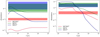 |
Fig. A.1 Same as Fig. 7, but assuming a cosmic-ray ionisation rate ζ = 1.3 × 10⁻¹⁴ s−1. |
| In the text | |
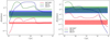 |
Fig. A.2 Same as Fig. A.1, but for ζ = 1.3 × 10⁻¹⁵ s−1. |
| In the text | |
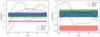 |
Fig. A.3 Same as Fig. A.1, but for ζ = 1.3 × 10⁻¹⁶ s−1. |
| In the text | |
Current usage metrics show cumulative count of Article Views (full-text article views including HTML views, PDF and ePub downloads, according to the available data) and Abstracts Views on Vision4Press platform.
Data correspond to usage on the plateform after 2015. The current usage metrics is available 48-96 hours after online publication and is updated daily on week days.
Initial download of the metrics may take a while.