| Issue |
A&A
Volume 651, July 2021
|
|
|---|---|---|
| Article Number | A15 | |
| Number of page(s) | 7 | |
| Section | Cosmology (including clusters of galaxies) | |
| DOI | https://doi.org/10.1051/0004-6361/202140595 | |
| Published online | 05 August 2021 | |
The Cosmic Large-Scale Structure in X-rays (CLASSIX) Cluster Survey
II. Unveiling a pancake structure with a 100 Mpc radius in the local Universe⋆
1
Universitäts-Sternwarte München, Fakultät für Physik, Ludwig-Maximilians-Universität München, Scheinerstr. 1, 81679 München, Germany
2
Max-Planck-Institut für Extraterrestrische Physik, 85748 Garching, Germany
e-mail: This email address is being protected from spambots. You need JavaScript enabled to view it.
Received:
17
February
2021
Accepted:
23
March
2021
Abstract
Previous studies of the galaxy and galaxy cluster distribution in the local Universe found indications for a large extension of the Local Supercluster up to a radius of 190 h70−1 Mpc. We are using our large and highly complete CLASSIX survey of X-ray luminous galaxy clusters detected in the ROSAT All Sky Survey to trace the matter distribution in the local Universe and to explore the size of the flattened local density structure associated with the Local Supercluster. The Local Supercluster is oriented almost perpendicular to the Galactic plane. Since Galactic extinction increases towards the Galactic plane, objects are on average more easily visible perpendicular to the plane than close to it, also producing an apparent concentration of objects along the Local Supercluster. We can correct for this bias by a careful treatment of the survey selection function. We find a significant overdensity of clusters in a flattened structure along the Supergalactic plane with a thickness of about 50 Mpc and an extent of about 100 Mpc radius. Structures at a distance larger than 100 Mpc are not correlated to the Local Supercluster any more. The matter density contrast of the local superstructure to the surroundings is about a factor of 1.3−2.3. Within the Supergalactic plane the matter is concentrated mostly in two superclusters, the Perseus-Pices Chain and Hydra-Centaurus supercluster. We have shown in our earlier work that the local Universe in a region with a radius of 100−170 Mpc has a lower density than the cosmic mean. For this reason, the Local Supercluster is not overdense with respect to the cosmic mean density. Therefore this local superstructure will not collapse as a whole in the future, but rather fragment.
Key words: galaxies: clusters: general / cosmology: observations / large-scale structure of Universe / X-rays: galaxies: clusters
Based on observations at the European Southern Observatory La Silla, Chile and the German-Spanish Observatory at Calar Alto.
© H. Böhringer et al. 2021
 Open Access article, published by EDP Sciences, under the terms of the Creative Commons Attribution License (https://creativecommons.org/licenses/by/4.0), which permits unrestricted use, distribution, and reproduction in any medium, provided the original work is properly cited.
Open Access funding provided by Max Planck Society.
1. Introduction
Our local neighbourhood in the Universe is characterised by a flattened matter density distribution which seems to show coherence over a hierarchy of scales. Studying the density distribution of bright galaxies in the sky, notably those compiled in the Shapley-Ames galaxy survey, De Vaucouleurs noted a concentration of these galaxies towards a plane roughly perpendicular to the plane of our Galaxy (de Vaucouleurs 1953, 1956, 1958, 1959). He called this pronounced structure the ‘Local Supergalactic System’, which is now referred to as the Local Supercluster. The system includes a number of galaxy groups and the Virgo cluster as its dominant member. This concentration of galaxies was noted earlier by William Herschel (see Flin 1986; Rubin 1951 for a historical account).
Already at much smaller scales, there is a pronounced segregation of galaxies towards the Supergalactic plane. The analysis of the galaxy distribution within a radius of about 6.5 Mpc by Courtois et al. (2013), for example, shows that almost all the nearby groups of galaxies, including the Local Group, the groups marked by IC 342, M 81, Cen A, M 83, N4214, and the Canes Venatici I and Maffei I groups, are contained in a very narrow slice, which is aligned with the Local Supercluster (see their Fig. 3). Other studies have found that this flattened structure also reaches far beyond the Local Supercluster. For example, Shaver & Pierre (1989) found in the distribution of nearby bright radio galaxies an indication of a concentration of these objects towards the Supergalactic Plane with an extent up to about a redshift of z ∼ 0.02 ( Mpc). Investigating the distribution of 48 nearby Abell clusters, Tully (1986, 1987) described a concentration which extends the Local Supercluster to a flattened superstructure with a diameter of about 360
  Mpc, stating that the orientation of the short axis is coinciding with the pole of the plane of the traditional Local Supercluster.
One problem for a quantitative mapping of the local superstructure is, however, the fact that observations are affected by Galactic absorption and extinction, which depend strongly on Galactic latitude. Since the Supergalactic plane is almost perpendicular to the Galactic disk, the Supergalactic poles are not affected by strong extinction while the Supergalactic plane is partly shaded by the Galactic band. This can lead to an apparent enhancement of the galaxy concentration towards the Supergalactic plane. We therefore reapproached the mapping of the local superstructure with tracer objects, for which such sampling bias can be avoided or properly corrected for.
For this reason, we used galaxy clusters to trace the large-scale structure. As an integral part of the cosmic large-scale structure, galaxy clusters are reliable tracers of the underlying dark matter distribution. Since they form from the largest peaks in the initially random Gaussian density fluctuation field, their density distribution can be statistically closely related to the matter density distribution (e.g. Bardeen et al. 1986). Cosmic structure formation theory has shown that the ratio of the cluster density fluctuation amplitude is enhanced with respect to the matter density fluctuations in the sense that the cluster density fluctuations follow the matter density fluctuations with a higher amplitude. The ratio of the amplitude of the cluster density to that of the dark matter is practically independent of the scale (Kaiser 1986; Mo & White 1996; Sheth & Tormen 1999). The fact that the cluster density fluctuation amplitude is enhanced makes clusters sensitive tracers of the matter distribution.
We used the large, highly complete sample of X-ray luminous galaxy clusters from the CLASSIX (Cosmic Large-Scale Structure in X-rays) galaxy cluster survey to probe the matter distribution in the nearby Universe. The detection of the objects in X-rays provides the advantage of X-ray emission ensuring that the systems are tight three-dimensional mass concentrations, and the X-ray luminosity provides a good estimate of the object’s mass. Therefore, by construction, an X-ray flux limited survey is practically mass selected (with some scatter) with a well-defined mass limit as a function of redshift. These properties of the survey are essential for the goal of this study. We have already applied CLASSIX to successful studies of the cosmic large-scale structure as described in Sect. 2 and the present study can build on this experience.
The paper is structured as follows. In Sect. 2 we describe the construction and properties of the CLASSIX galaxy cluster survey and some relevant applications. Section 3 deals with some methodological issues. The results of our analysis is presented in Sect. 4 and implications are discussed in Sect. 5. Section 6 provides a summary and conclusions. For physical properties, which depend on distance, we use the following cosmological parameters: a Hubble constant of H0 = 70 km s−1 Mpc−1, a matter density, Ωm = 0.3, and a spatially flat metric. For the cosmographical analysis, we use Supergalactic coordinates, defined by the location of the Supergalactic North Pole at lII = 47.3700 deg and bII = 6.3200 deg, consistent with the definition by de Vaucouleurs et al. (1991) in the Third Catalog of Bright Galaxies (see also Lahav et al. 2000).
2. The CLASSIX galaxy cluster survey
This study requires a cluster catalogue that traces the local Universe densely enough, is statistically highly complete, and has a well-known selection function. At the moment, the best data base is the CLASSIX galaxy cluster catalogue (Böhringer et al. 2016). It is the combination of our surveys in the southern sky, REFLEX II (Böhringer et al. 2013), and the northern hemisphere, NORAS II (Böhringer et al. 2017). Together they cover 8.26 ster of the sky at galactic latitudes |bII|≥20° and the cluster catalogue contains 1773 members. In this study, we do not excise the regions of the Magellanic Clouds or the VIRGO cluster. In the complete survey, we find no significant deficit in the cluster density in these sky areas. We also used an extension of CLASSIX to lower galactic latitudes into the ‘zone of avoidance’ (ZoA). This region is restricted to the area with an interstellar hydrogen column density nH ≤ 2.5 × 1021 cm−2, because in regions with a higher column density, X-rays are strongly absorbed and usually the sky has a high stellar density, making the detection of clusters in the optical extremely difficult. The values for the interstellar hydrogen column density are taken from the 21 cm survey of Dickey & Lockman (1990)1. This area amounts to another 2.56 ster and altogether the survey data cover 86.2% of the sky. The spectroscopic follow-up to obtain redshifts for this part of the survey is about 70% complete and also the completeness of the cluster sample is not as high as for REFLEX and NORAS. The cluster density we used for the ZoA is therefore a lower limit. In total, we have 143 galaxy clusters with a redshift z ≤ 0.03 and an X-ray luminosity LX ≥ 1042 erg s−1 that we use in this study.
The CLASSIX galaxy cluster survey and its extension is based on the X-ray detection of galaxy clusters in the ROSAT All-Sky Survey (RASS, Trümper 1993; Voges et al. 1999). The source detection for the survey, the construction of the survey, and the survey selection function as well as tests of the completeness of the survey are described in Böhringer et al. (2013, 2017). In summary, the nominal unabsorbed flux limit for the galaxy cluster detection in the RASS is 1.8 × 10⁻¹² erg s−1 cm−2 in the 0.1−2.4 keV energy band. For the assessment of the large-scale structure in this paper, we apply an additional cut on the minimum number of detected source photons of 20 counts. This has the effect that the nominal flux limit quoted above is only reached in about 80% of the survey. In regions with lower exposure and higher interstellar absorption, the flux limit is accordingly higher (see Fig. 11 in Böhringer et al. 2013 and Fig. 5 in Böhringer et al. 2017). This effect is modelled and taken into account in the survey selection function.
We have already demonstrated with the REFLEX I survey (Böhringer et al. 2004) that clusters provide a precise means to obtain a census of the cosmic large-scale matter distribution through, for example, the correlation function (Collins et al. 2000), the power spectrum (Schuecker et al. 2001, 2002, 2003a,b), Minkowski functionals (Kerscher et al. 2001), and, using REFLEX II, with the study of superclusters (Chon & Böhringer 2013; Chon et al. 2014) and the cluster power spectrum (Balaguera-Antolinez et al. 2011, 2012). The latter study also demonstrates that the theoretically predicted large-scale structure bias, that is the amplification factor, with which the clusters trace the matter density fluctuations is confirmed by observations.
Relevant physical parameters for clusters were determined in the following way. X-ray luminosities in the 0.1−2.4 keV energy band were derived within a cluster radius of r5002. To estimate the cluster mass and temperature from the observed X-ray luminosity, we used the scaling relations described in Pratt et al. (2009). They were determined from a representative cluster sub-sample of our survey, called REXCESS (Böhringer et al. 2007) which was studied in detail with deep XMM-Newton observations. Since the radius r500 was determined from the cluster mass, the calculation of X-ray luminosity inside r500, the cluster mass, and temperature were performed iteratively, as described in Böhringer et al. (2013). The definitive identification of the clusters and the redshift measurements are described in Guzzo et al. (2009), Chon & Böhringer (2012), and Böhringer et al. (2013).
The survey selection function was determined as a function of the sky position with an angular resolution of one degree and as a function of redshift. The selection function takes all the systematics of the RASS exposure distribution, galactic absorption, and the detection photon count limit into account. The interstellar hydrogen column density for these calculations is taken from Dickey & Lockman (1990). The selection function as a function of the sky position and redshift was published for REFLEX II in the online material of Böhringer et al. (2013) and for NORAS II in Böhringer et al. (2017).
3. Method
We studied the density distribution of clusters and of the underlying matter distribution as a function of redshift in different regions of the sky. Because we used a flux-limited cluster sample with additional smaller sensitivity variations in regions of the sky with shorter exposures, the survey selection function has to be taken into account to derive the cluster density distribution. In the following, we describe the method used to correct for the selection effects.
We assigned weights to each cluster to correct for the spatially varying survey limits. The weights were calculated from an integration of the luminosity function, ϕ(LX), as follows:
 (1)
(1)
where LX0 is the nominal lower limit of the sample and LXi is the lower X-ray luminosity limit at the sky location and redshift of the cluster. The adopted X-ray luminosity function was determined in Böhringer et al. (2014). To calculate the cluster density, we summed up the weights for each cluster involved, which provides the estimated cluster density for a volume-limited survey with a lower luminosity limit of LX0. This method was used to produce the cluster density maps on the sky in the next section. We use a value of 1042 erg s−1 for LX0 throughout the paper.
4. Results
4.1. Sky distribution
A first impression of the distribution of nearby X-ray luminous galaxy clusters is provided by their location on the sky, as shown in Fig. 1. The upper panel shows the cluster distribution out to a redshift of z = 0.02 (a distance of about 85.3 Mpc). The Supergalactic band with a width of 20° above and below the Superglatic plane is marked. The region with high galatic absorption (nH ≥ 2.5 × 1021 cm−2) is marked in white in the colour coding and the few clusters in this region are not considered. The thin, nearly horizontal lines indicate Galactic latitudes bII = ±20°. In total, 69 CLASSIX clusters fall into the study region, of which 17 are located in the ZoA. We used the method described in Sect. 3 to create a map of the surface density distribution of clusters smoothed with a Gaussian filter on a scale of 10°. This map, shown in the figure, was normalised to the mean density. Bright areas show overdensities (orange: R > 2, light red: R = 1−2, where R is the density ratio to the mean density), while dark regions are underdense (light brown: R = 0.5−1, dark brown and black: R < 0.5). The bright regions are located in and near to the Supergalactic band. There is no comparably dense region outside the Supergalactic band. Most of the clusters are found in two major concentrations inside the Supergalactic band. These are the Perseus-Pisces supercluster and the neighbouring Southern Great Wall in the Cetus region (in the lower left quadrant) and the Hydra-Centaurus supercluster (around Galactic longitude 315° and latitude 0−40°).
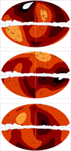 |
Fig. 1. Sky distribution of the CLASSIX galaxy clusters in the redshift range z = 0−0.02 (top panel), z = 0.02−0.025 (middle), and z = 0.025−0.03 (bottom) in Galactic coordinates. Clusters inside the Supergalactic band at latitudes ≤ ± 20° are shown as filled circles, while all other clusters are displayed as open circles. The solid lines show Supergalactic latitudes ±20° and the dashed line shows the Supergalactic equator. The coloured map shows the cluster surface density as explained in the text. |
The middle panel of Fig. 1 shows the CLASSIX cluster distribution in the next outer shell at z = 0.02−0.025. The concentration of clusters seen near the North Galactic Pole is the part of the Great Wall that falls into this redshift shell. This includes the Coma cluster as well as Abell 1367. The regions outside the Supergalactic band are mostly occupied by underdense regions. In the next outer redshift shell at z = 0.025−0.03, which is shown in the bottom panel of Fig. 1, the densest region is no longer close to the Supergalactic plane and major underdense regions fall into the Supergalactic band. Thus the segregation of massive structures towards the Supergalactic plane does not extend further than a distance of about z = 0.025 (∼106 Mpc). The concentration of clusters seen in this panel consists of groups and clusters not far from the Hercules supercluster, which is at a slightly larger distance.
In Fig. 2 we show the CLASSIX cluster distribution at redshifts z ≤ 0.02 again and compare it to the distribution of galaxies from the 2MASS redshift survey (Huchra et al. 2012) in the same redshift region. We can clearly see that the cluster concentrations coincide with the densest regions in the galaxy distribution, which is an indication that both are presumably good tracers of the distribution of dark matter.
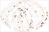 |
Fig. 2. Sky distribution of the CLASSIX galaxy clusters in the redshift range z = 0−0.02 in equatorial coordinates. Clusters in the ZoA are shown as open circles, while all other clusters are marked with filled circles. The small brown dots show the galaxies from the 2MASS redshift survey (Huchra et al. 2012) in the same redshift range. The two black dotted lines show Galactic latitudes of bII = ±20°, the blue lines show the boundaries of the zone of high galactic absorption with a hydrogen column density nH ≥ 2.5 × 1021 cm−2, and the two solid red lines show the Supergalactic latitudes ±20°. |
To quantify the concentration of clusters towards the Supergalactic plane, in Fig. 3 we plotted the surface density of the clusters on the sky as a function of Supergalactic latitude in the redshift region z = 0−0.02. Shown is the overdensity of clusters in a region for a given maximum Supergalactic latitude, which was determined as the ratio of the surface density of clusters in this region to the mean density in the full survey area in the given redshift range. There is a strong concentration of clusters at latitudes inside ±10° with wings of the distribution out to about ±30°. The figure shows the results for two cluster samples. The upper plot only considers the clusters at |bII|≥20°, where the survey is complete and the selection function is precise. But this sample covers only 66% of the sky. In the lower panel, the survey is extended into the ZoA covering 86.2% of the sky, but the survey completeness and the selection function are not well known in the added area, and therefore the result is more qualitative. Nevertheless, it shows that there is no prominent structure hidden in the ZoA that would significantly change the result shown in the upper panel.
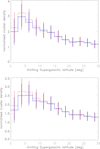 |
Fig. 3. Sky surface density ratio of the CLASSIX clusters at z = 0−0.02 in a sky area limited by a maximum Supergalactic latitude, |bSG|, compared to the mean surface density in the full volume at z = 0−0.02. The solid blue curve shows the density determined with weights correcting for the sensitivity variations in the survey as explained in the text, while the dashed red line gives the unweighted density ratio. The meaning of the error bars is explained in Sect. 4.1. Top panel: results for the region outside the ZoA, bottom panel: results for the full sky region with hydrogen absorption column density nH ≤ 25 × 1020 cm−2. |
The error bars shown in the plots are Poisson uncertainties of the cluster number counts. We note that these are not to be interpreted as measurement uncertainties since the cluster surface density is what was measured directly without errors. If the occurrence of clusters in this distribution is interpreted as a Poisson point process realisation of the density values of an underlying density field, then these error bars provide the uncertainty, with which this underlying density field is represented by the clusters. In astrophysical terms, it is the accuracy with which the underlying matter density field can be traced by galaxy clusters. The same interpretation applies to the error bars shown in Figs. 4–6.
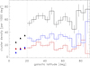 |
Fig. 4. Surface density of the CLASSIX galaxy clusters on the sky as a function of galactic latitude, |bII|. The black histogram shows all clusters, while the red one shows clusters in the redshift range z = 0.−0.07 and the blue one clusters at z = 0.07−0.2. No clusters are detected closer than five degrees to the Galactic plane due to the restriction to the region with nH ≤ 2.5 × 1021 cm−2. The dotted line shows the boundary of the ZoA. Inside this boundary, we provide lower limits for the cluster density since the redshift survey is incomplete there. |
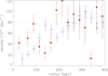 |
Fig. 5. Comparison of the density of CLASSIX galaxy clusters in a slice of 50 Mpc width around the Supergalactic plane (red, filled data points) to the region outside (blue, open data points). Only the volume and the data outside the ZoA are considered. The densities were determined in concentric shells with a radial width of 25 Mpc. The cluster densities were multiplied with a correction factor to account for survey sensitivity variations. The mean density in the survey volume out to 400 Mpc is indicated as a dotted line. |
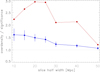 |
Fig. 6. Overdensity of galaxy clusters in a slice of half width as specified on the X-axis with respect to the mean density in the survey within a sphere of 100 Mpc radius (lower curve with error bars). For the meaning of the error bars, readers can consult the text in Sects. 4.1 and 4.2. The upper curve indicates the significance of the existence of an overdensity in the underlying matter density distribution. |
It is important for this investigation that there is no selection bias of clusters as a function of galactic latitude, at least outside the ZoA. Thus we show in Fig. 4, that we find no significant decrease in the surface density with decreasing galactic latitude for |bII|> 20°. For this study we chose two redshift bins with sufficient statistics containing 608 (943) clusters for z = 0−0.07 (z = 0.07−0.2), respectively. The variations in the surface density are larger than the error bars, determined from Poisson counting statistics. This should be attributed to large-scale structure since we do not see the same variations if we look at the surface brightness in different redshift shells as shown in Fig. 4. At galactic latitudes |bII|< 20°, we give only lower limits in the figure since there, in the ZoA, the survey is incomplete.
4.2. Radial extent and width of the superstructure
The next goal is to obtain a quantitative measure of the density contrast and extent of the overdense structure in three dimensions. With this objective, we compared the cluster density inside a slice of ±25 Mpc around the Supergalactic plane to the density outside. To explore the radial extent of the overdensity in the slice, we divided the space into spherical shells with a radial width of 25 Mpc. In each shell, we determined the cluster density in the part of the shell which is contained in the slice as well as the cluster density outside the slice. We show the results in Fig. 5. For the outer region, there is no contributing volume for the innermost sphere of 25 Mpc radius and therefore no data point. For the inner region, we combined the first two bins to increase the otherwise poor statistics. The cluster density was corrected with cluster weights determined by means of the survey selection function. The mean density inside the survey volume out to 400 Mpc is indicated by the dotted line.
We note first that the densities are low at small radii. This result has been studied in Böhringer et al. (2020), where we find a significant local matter underdensity in the Universe out to a radius of about 170 Mpc. Outside this radius, there is a compensating overdensity due to the presence of several superclusters, the most prominent of which is the Shapley supercluster. Considering the comparison of the cluster density in the two local regions, we find that the region close to the Supergalactic plane has a significantly higher density than the outer region in all bins inside a radius of 100 Mpc. Outside this radius, the density ratio reverses for the next two bins. Thus we clearly observe that the flattened structure of the extended Local Supercluster stretches out to about 100 Mpc and there is no coherence with this structure at larger radii.
For the calculation in Fig. 5, we used the data in the volume outside the ZoA. Including the ZoA in this analysis yields a similar result with a slightly larger overdensity of the region around the Supergalactic plane.
To characterise the width of the flattened local superstructure, we repeated the study shown in Fig. 5 for a number of half-width parameters ranging from 10 to 50 Mpc. In all cases, we determined the overdensity of the flattened superstructure with respect to the mean density of the full survey volume out to a radial distance of 100 Mpc. The results are shown in Fig. 6 where we note an increasing overdensity with a decreasing width. The data points directly show the observed cluster density, while the error bars give again the uncertainty of any implications drawn for the underlying density field. The same meaning is also relevant for the significance of the overdensity, also given in the figure. We note that overall the overdensity and its significance is large up to a width of about 50 Mpc, and we adopt this value to best characterise the extent of the local superstructure perpendicular to the Supergalactic plane. The significance of the overdensity in the dark matter distribution inferred from the cluster sample is about 2.9σ (Fig. 6).
4.3. Three-dimensional cluster distribution
To illustrate the three-dimensional cluster distribution in Supergalactic coordinates, we used the visualisation presented in Fig. 7, which shows the CLASSIX clusters used in this study located inside a radius of 100 Mpc. The clusters located in the Supergalactic structure in a slice with a width of 50 Mpc are shown with filled blue circles and filled green squares. The remaining clusters are marked with red open symbols. We note that most of the clusters are contained in the two concentrations (as already noted in Figs. 1 and 2) associated with the Perseus-Pisces supercluster and the Southern Great Wall next to it, which appears on the right in Fig. 7, and the Hydra-Centaurus supercluster on the left.
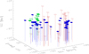 |
Fig. 7. Visualisation of the three-dimensional distribution of the CLASSIX galaxy clusters in Supergalactic coordinates within a radius of 100 Mpc. The clusters within a slice of 50 Mpc width around the Supergalactic plane are marked with filled blue circles and filled green squares, the clusters outside are shown with red open symbols. We note two major cluster concentrations associated with the Perseus-Pisces supercluster together with the Southern Great Wall (on the right) and Hydra-Centaurus supercluster (on the left). The cluster members of the Great Wall in the slice are marked with green squares. We also show four further members of the Great Wall inside the slice, but just outside the 100 Mpc boundary with green open squares. |
Using a variable linking length with a minimum value of 19 Mpc and a dynamical correction using the weighting factors at each cluster location (a more detailed analysis and description will be given in a forthcoming paper), we constructed memberships to local superclusters. The superclusters found with at least four members inside a radius of 100 Mpc are Perseus-Pisces with 17 members (of which 13 are located in the 50 Mpc wide slice and five additional clusters are connected to it outside the 100 Mpc radius), the Southern Great Wall with five members (where one cluster is located outside the slice and two additional clusters are connected outside 100 Mpc), the Centaurus supercluster with ten members (all located in the slice), the local concentration around Virgo with five members, and parts of the Great Wall. Five clusters of the Great Wall are located inside the slice, four clusters are located outside the slice, and four further clusters are found at a distance between 100 and 132 Mpc. In Fig. 7 we show the Great Wall members inside the slice around the Supergalactic plane with different symbols (green squares) to better distinguish them from the Centaurus Supercluster. In this volume with a radius of 100 Mpc, 52% of all CLASSIX clusters are contained in the two major superstructures, the Perseus-Pisces and Southern Great Wall complex as well as the Centaurus supercluster. If we add the clusters around Virgo and in the Great Wall, 70% would belong to superstructures. More details of these structures and their member clusters will be the subject of a forthcoming paper.
The Great Wall appears only partly at the edge of the volume with r ≤ 100 Mpc. To show the extension of the Great Wall near the Supergalatic Plane, we also display the four clusters inside the slice, but at radii of 100−132 Mpc with open, green squares. The local superstructure described by Tully et al. (2014) as the Laniakea supercluster comprises the local Supercluster including Virgo, the Hydra-Centaurus supercluster, and some clusters close to these systems and it makes up most of the concentration seen in the middle and left part of Fig. 7.
5. Discussion
We found a strong concentration of the cluster density towards the Supergalactic plane in a region with a radial extent of about 100 Mpc. Previously, we found the same region to be underdense with respect to the mean density of the Universe on larger scales (Böhringer et al. 2015, 2020). Inspecting Fig. 5, we note that even though the slice of the local superstructure is locally significantly overdense, its density is still less than the mean cosmic matter density on large scales. The inner part of this structure, characterised by Tully and his collaborators as the Laniakea supercluster (Tully et al. 2014) has also slightly less than a mean density as pointed out by Chon et al. (2015). In consequence, this large, apparently coherent structure is not gravitationally bound and will not collapse in the future to one large massive system, but rather disperse into several distinct structures in the frame of ΛCDM cosmology (Chon et al. 2015). As part of this structure, our Local Group, which has a distinct peculiar velocity towards the Virgo cluster, will finally not end up in a large mass concentration, but it will remain quite isolated when large fractions of the local superstructure collapse into massive matter concentrations.
For the concentration of clusters towards the Supergalactic plane, we found a density contrast of about a factor of 1.5 with respect to the mean density in a slice of half width of 25 Mpc and a radius of about 100 Mpc (Fig. 6). In projection, the density contrast in a sky region with a width of about 10−20° around the Supergalactic equator out to a distance of about 85 Mpc was even larger with a factor of about 2.5 to 3 (Fig. 3). The extent of the region in latitude corresponds to a width of the slice at z = 0.02 of about ±7−14 Mpc. The larger number in the latter case is partly due to the measurement within a smaller radius and partly due to a more favourable geometry.
In the present study, we excluded the sky region with high interstellar absorption, which constitutes about 13.8% of the sky. In addition the survey in the ZoA is incomplete. The latter effect should be small at the relevant low redshifts, however, as nearby clusters are more easily detected and we have given a higher priority to the follow-up of low redshift clusters. This is also reflected in Fig. 4, where we can see no severe deficit of clusters at low galactic latitudes for the low redshift clusters compared to the high redshift sample. Even if we make the extreme assumption that we have missed more than half the clusters in the ZoA and that all of these are located outside the local structure, the significance for the overdense pancake with a thickness of 50 Mpc would only decrease from over 3σ to about 2.7σ. The ongoing eROSITA survey could help to find some of the missing clusters. But with the above statistics, we do not expect that including all groups and clusters possibly hidden in the ZoA would change the conclusion of our study.
Since we have shown with simulations in our earlier study (Böhringer et al. 2020) that clusters are true tracers of the underlying matter distribution and that Poisson statistics provides a fair account of the accuracy with which the density variation can be determined on large scales, we can draw conclusions on the matter density contrast that is involved in this cosmographical mapping. For this, we have to take into account that galaxy clusters are biased tracers of the mass distribution in the sense that the density contrast seen in the clusters is enhanced by a certain bias factor with respect to the underlying matter distribution. The bias factor can be derived approximately, as shown in our earlier study (Böhringer et al. 2020), where we make use of the theoretical bias relations determined on the basis of large cosmological N-body simulations, for example by Tinker et al. (2010). For the lower mass limit of 2−3.5 × 10¹³ M⊙ for the CLASSIX survey in the redshift range z = 0−0.235, we estimate bias factors of ∼1.4−1.7 (for the lower and higher redshift regions, respectively). The bias of the cluster density is defined as  , where RCL is the cluster density contrast and ΔCL and ΔDM are the cluster and matter overdensity, respectively. Therefore the result implies a density contrast in the matter distribution for the local superstructure slice of RDM = ΔDM + 1 = (RCL − 1)/b + 1, which is about 1.3 to 2.3, with RCL taken from Figs. 3 and 6, respectively.
6. Summary and conclusion
We have shown by means of the distribution of X-ray luminous clusters that the matter distribution in the local Universe shows a strong segregation towards the Supergalactic plane. This segregation is present on small scales of about 6 Mpc in the distribution of local galaxy groups. It continues in the geometry of the Local Supercluster and extends out to a radius of about 100 Mpc. At the largest scales, this local superstructure is well traced by X-ray luminous galaxy groups and clusters. Perpendicular to the Supergalactic plane, the structure has a width of about 50 Mpc inside which the cluster density contrast is about a factor of 1.5−3 compared to the mean. This implies a density contrast in the matter distribution of about 1.3 to 2.3.
Inside the flattened superstructure, the clusters are mostly concentrated in three major superclusters: the Hydra-Centaurus complex which has a connection to the Local Supercluster, the Perseus-Pisces supercluster with a connection to the Southern Great Wall, and part of the Great Wall. More than half of the clusters in the local Universe belong to these superclusters. This is similar to the finding of Chon et al. (2014) studying the fraction of clusters in superclusters in simulations. As shown previously, this local region of the Universe is less dense than the global mean. Therefore, even if the flat superstructure has a higher density than the local mean, it is not dense enough to collapse in the future into one structure within the standard ΛCDM cosmological scenario. It will rather fragment into several pieces, where only the core regions of the superclusters involved will form the largest future objects.
We have compared the interstellar hydrogen column density compilation by Dickey & Lockman (1990) with the more recent data set of the Bonn-Leiden-Argentine 21 cm survey (Kalberla et al. 2005) and found that the differences relevant for us are of the order of at most one percent. Because our survey was constructed with a flux cut based on the Dickey & Lockman results, we kept the older hydrogen column density values for consistency reasons.
r500 is the radius where the average mass density inside reaches a value of 500 times the critical density of the Universe at the epoch of observation.
Acknowledgments
We thank the referee for helpful comments. We acknowledge support by the DFG through the Munich Excellence Cluster Universe. G.C. acknowledges support by the DLR under grant no. 50 OR 1905.
References
- Balaguera-Antolinez, A., Sanchez, A., Böhringer, H., et al. 2011, MNRAS, 413, 386 [NASA ADS] [CrossRef] [Google Scholar]
- Balaguera-Antolinez, A., Sanchez, A., Böhringer, H., et al. 2012, MNRAS, 425, 2244 [NASA ADS] [CrossRef] [Google Scholar]
- Bardeen, J. M., Bond, J. R., Kaiser, N., et al. 1986, ApJ, 304, 15 [NASA ADS] [CrossRef] [Google Scholar]
- Böhringer, H., Schuecker, P., Guzzo, L., et al. 2004, A&A, 425, 367 [NASA ADS] [CrossRef] [EDP Sciences] [Google Scholar]
- Böhringer, H., Schuecker, P., Pratt, G. W., et al. 2007, A&A, 469, 363 [NASA ADS] [CrossRef] [EDP Sciences] [Google Scholar]
- Böhringer, H., Chon, G., Collins, C. A., et al. 2013, A&A, 555, A30 [NASA ADS] [CrossRef] [EDP Sciences] [Google Scholar]
- Böhringer, H., Chon, G., Collins, C. A., et al. 2014, A&A, 570, A31 [NASA ADS] [CrossRef] [EDP Sciences] [Google Scholar]
- Böhringer, H., Chon, G., Bristow, M., et al. 2015, A&A, 574, A26 [NASA ADS] [CrossRef] [EDP Sciences] [Google Scholar]
- Böhringer, H., Chon, G., & Kronberg, P. P. 2016, A&A, 596, A22 [NASA ADS] [CrossRef] [EDP Sciences] [Google Scholar]
- Böhringer, H., Chon, G., Retzlaff, J., et al. 2017, AJ, 153, 220 [NASA ADS] [CrossRef] [Google Scholar]
- Böhringer, H., Chon, G., & Collins, C. A. 2020, A&A, 633, A19 [EDP Sciences] [Google Scholar]
- Chon, G., & Böhringer, H. 2012, A&A, 538, A35 [NASA ADS] [CrossRef] [EDP Sciences] [Google Scholar]
- Chon, G., & Böhringer, H. 2013, MNRAS, 429, 3272 [NASA ADS] [CrossRef] [Google Scholar]
- Chon, G., Böhringer, H., Collins, C. A., et al. 2014, A&A, 567, A144 [NASA ADS] [CrossRef] [EDP Sciences] [Google Scholar]
- Chon, G., Böhringer, H., & Zaroubi, S. 2015, A&A, 575, L14 [NASA ADS] [CrossRef] [EDP Sciences] [Google Scholar]
- Collins, C. A., Guzzo, L., Böhringer, H., et al. 2000, MNRAS, 319, 939 [NASA ADS] [CrossRef] [Google Scholar]
- Courtois, H. M., Pomàrede, D., Tully, R. B., et al. 2013, AJ, 146, 69 [NASA ADS] [CrossRef] [Google Scholar]
- de Vaucouleurs, G. 1953, AJ, 58, 30 [NASA ADS] [CrossRef] [Google Scholar]
- de Vaucouleurs, G. 1956, Vistas Astron., 2, 1584 [NASA ADS] [CrossRef] [Google Scholar]
- de Vaucouleurs, G. 1958, ApJ, 63, 223 [Google Scholar]
- de Vaucouleurs, G. 1959, Sov. Astron., 3, 897 [NASA ADS] [Google Scholar]
- de Vaucouleurs, G., de Vaucouleurs, A., Corwin, H. G., Jr., et al. 1991, The Third Catalogue of Bright Galaxies (RC3) (Austin: University of Texas Press) [Google Scholar]
- Dickey, J. M., & Lockman, F. J. 1990, ARA&A, 28, 215 [NASA ADS] [CrossRef] [MathSciNet] [Google Scholar]
- Flin, P. 1986, Acta Cosmol., 14, 7 [Google Scholar]
- Guzzo, L., Schuecker, P., Böhringer, H., et al. 2009, A&A, 499, 357 [NASA ADS] [CrossRef] [EDP Sciences] [Google Scholar]
- Huchra, J. P., Macri, L. M., Masters, K. L., et al. 2012, ApJS, 199, 26 [NASA ADS] [CrossRef] [Google Scholar]
- Kaiser, N. 1986, ApJ, 284, L9 [Google Scholar]
- Kalberla, P. M. W., Burton, W. B., Hartmann, D., et al. 2005, A&A, 440, 775 [NASA ADS] [CrossRef] [EDP Sciences] [Google Scholar]
- Kerscher, M., Mecke, K., Schuecker, P., et al. 2001, A&A, 377, 1 [NASA ADS] [CrossRef] [EDP Sciences] [Google Scholar]
- Lahav, O., Santiago, B. X., Webster, A. M., et al. 2000, MNRAS, 312, 166 [NASA ADS] [CrossRef] [EDP Sciences] [Google Scholar]
- Mo, H. J., & White, S. D. M. 1996, MNRAS, 282, 347 [Google Scholar]
- Pratt, G. W., Croston, J. H., Arnaud, M., & Böhringer, H. 2009, A&A, 498, 361 [NASA ADS] [CrossRef] [EDP Sciences] [Google Scholar]
- Rubin, V. 1951, AJ, 56, 47 [NASA ADS] [CrossRef] [Google Scholar]
- Schuecker, P., Böhringer, H., Guzzo, L., et al. 2001, A&A, 368, 86 [NASA ADS] [CrossRef] [EDP Sciences] [Google Scholar]
- Schuecker, P., Guzzo, L., Collins, C. A., et al. 2002, MNRAS, 335, 807 [NASA ADS] [CrossRef] [EDP Sciences] [Google Scholar]
- Schuecker, P., Böhringer, H., Collins, C. A., et al. 2003a, A&A, 398, 867 [NASA ADS] [CrossRef] [EDP Sciences] [Google Scholar]
- Schuecker, P., Caldwell, R. R., Böhringer, H., et al. 2003b, A&A, 402, 53 [NASA ADS] [CrossRef] [EDP Sciences] [Google Scholar]
- Shaver, P. A., & Pierre, M. 1989, A&A, 220, 35 [Google Scholar]
- Sheth, R. K., & Tormen, G. 1999, MNRAS, 308, 119 [NASA ADS] [CrossRef] [Google Scholar]
- Tinker, J. L., Robertson, B. E., & Kravtsov, A. V. 2010, ApJ, 724, 878 [NASA ADS] [CrossRef] [Google Scholar]
- Trümper, J. 1993, Science, 260, 1769 [NASA ADS] [CrossRef] [PubMed] [Google Scholar]
- Tully, R. B. 1986, ApJ, 303, 25 [NASA ADS] [CrossRef] [Google Scholar]
- Tully, R. B. 1987, ApJ, 321, 280 [NASA ADS] [CrossRef] [Google Scholar]
- Tully, R. B., Courtois, H., Hoffman, Y., et al. 2014, Nature, 513, 71 [NASA ADS] [CrossRef] [Google Scholar]
- Voges, W., Aschenbach, B., Boller, T., et al. 1999, A&A, 349, 389 [NASA ADS] [Google Scholar]
All Figures
|
Fig. 1. Sky distribution of the CLASSIX galaxy clusters in the redshift range z = 0−0.02 (top panel), z = 0.02−0.025 (middle), and z = 0.025−0.03 (bottom) in Galactic coordinates. Clusters inside the Supergalactic band at latitudes ≤ ± 20° are shown as filled circles, while all other clusters are displayed as open circles. The solid lines show Supergalactic latitudes ±20° and the dashed line shows the Supergalactic equator. The coloured map shows the cluster surface density as explained in the text. |
| In the text | |
|
Fig. 2. Sky distribution of the CLASSIX galaxy clusters in the redshift range z = 0−0.02 in equatorial coordinates. Clusters in the ZoA are shown as open circles, while all other clusters are marked with filled circles. The small brown dots show the galaxies from the 2MASS redshift survey (Huchra et al. 2012) in the same redshift range. The two black dotted lines show Galactic latitudes of bII = ±20°, the blue lines show the boundaries of the zone of high galactic absorption with a hydrogen column density nH ≥ 2.5 × 1021 cm−2, and the two solid red lines show the Supergalactic latitudes ±20°. |
| In the text | |
|
Fig. 3. Sky surface density ratio of the CLASSIX clusters at z = 0−0.02 in a sky area limited by a maximum Supergalactic latitude, |bSG|, compared to the mean surface density in the full volume at z = 0−0.02. The solid blue curve shows the density determined with weights correcting for the sensitivity variations in the survey as explained in the text, while the dashed red line gives the unweighted density ratio. The meaning of the error bars is explained in Sect. 4.1. Top panel: results for the region outside the ZoA, bottom panel: results for the full sky region with hydrogen absorption column density nH ≤ 25 × 1020 cm−2. |
| In the text | |
|
Fig. 4. Surface density of the CLASSIX galaxy clusters on the sky as a function of galactic latitude, |bII|. The black histogram shows all clusters, while the red one shows clusters in the redshift range z = 0.−0.07 and the blue one clusters at z = 0.07−0.2. No clusters are detected closer than five degrees to the Galactic plane due to the restriction to the region with nH ≤ 2.5 × 1021 cm−2. The dotted line shows the boundary of the ZoA. Inside this boundary, we provide lower limits for the cluster density since the redshift survey is incomplete there. |
| In the text | |
|
Fig. 5. Comparison of the density of CLASSIX galaxy clusters in a slice of 50 Mpc width around the Supergalactic plane (red, filled data points) to the region outside (blue, open data points). Only the volume and the data outside the ZoA are considered. The densities were determined in concentric shells with a radial width of 25 Mpc. The cluster densities were multiplied with a correction factor to account for survey sensitivity variations. The mean density in the survey volume out to 400 Mpc is indicated as a dotted line. |
| In the text | |
|
Fig. 6. Overdensity of galaxy clusters in a slice of half width as specified on the X-axis with respect to the mean density in the survey within a sphere of 100 Mpc radius (lower curve with error bars). For the meaning of the error bars, readers can consult the text in Sects. 4.1 and 4.2. The upper curve indicates the significance of the existence of an overdensity in the underlying matter density distribution. |
| In the text | |
|
Fig. 7. Visualisation of the three-dimensional distribution of the CLASSIX galaxy clusters in Supergalactic coordinates within a radius of 100 Mpc. The clusters within a slice of 50 Mpc width around the Supergalactic plane are marked with filled blue circles and filled green squares, the clusters outside are shown with red open symbols. We note two major cluster concentrations associated with the Perseus-Pisces supercluster together with the Southern Great Wall (on the right) and Hydra-Centaurus supercluster (on the left). The cluster members of the Great Wall in the slice are marked with green squares. We also show four further members of the Great Wall inside the slice, but just outside the 100 Mpc boundary with green open squares. |
| In the text | |
Current usage metrics show cumulative count of Article Views (full-text article views including HTML views, PDF and ePub downloads, according to the available data) and Abstracts Views on Vision4Press platform.
Data correspond to usage on the plateform after 2015. The current usage metrics is available 48-96 hours after online publication and is updated daily on week days.
Initial download of the metrics may take a while.