| Issue |
A&A
Volume 656, December 2021
|
|
|---|---|---|
| Article Number | A144 | |
| Number of page(s) | 26 | |
| Section | Cosmology (including clusters of galaxies) | |
| DOI | https://doi.org/10.1051/0004-6361/202141341 | |
| Published online | 15 December 2021 | |
The Cosmic Large-Scale Structure in X-rays (CLASSIX) Cluster Survey
IV. Superclusters in the local Universe at z ≤ 0.03⋆
1
Universitäts-Sternwarte München, Fakultät für Physik, Ludwig-Maximilians-Universität München, Scheinerstr. 1, 81679 München, Germany
2
Max-Planck-Institut für extraterrestrische Physik, 85748 Garching, Germany
e-mail: This email address is being protected from spambots. You need JavaScript enabled to view it.
Received:
18
May
2021
Accepted:
7
October
2021
Abstract
It is important to map the large-scale matter distribution in the local Universe for cosmological studies, such as the tracing of the large-scale peculiar velocity flow, the characterisation of the environment for different astronomical objects, and for precision measurements of cosmological parameters. We used X-ray luminous clusters to map this matter distribution and find that about 51% of the groups and clusters are members of superclusters which occupy only a few percent of the volume. In this paper we provide a detailed description of these large-scale structures. With a friends-to-friends algorithm, we find eight superclusters with a cluster overdensity ratio of at least two with five or more galaxy group and cluster members in the cosmic volume out to z = 0.03. The four most prominent ones are the Perseus-Pisces, the Centaurus, the Coma, and the Hercules supercluster, with lengths from about 40 to over 100 Mpc and estimated masses of 0.6 − 2.2 × 10¹⁶ M⊙. The largest of these structures is the Perseus-Pisces supercluster. The four smaller superclusters include the Local and the Abell 400 supercluster and two superclusters in the constellations Sagittarius and Lacerta. We provide detailed maps, member catalogues, and physical descriptions of the eight superclusters. By constructing superclusters with a range of cluster sub-samples with different lower X-ray luminosity limits, we show that the main structures are always reliably recovered.
Key words: galaxies: clusters: general / cosmology: observations / large-scale structure of Universe / X-rays: galaxies: clusters
Based on observations at the European Southern Observatory La Silla, Chile and the German-Spanish Observatory at Calar Alto.
© H. Böhringer and G. Chon 2021
 Open Access article, published by EDP Sciences, under the terms of the Creative Commons Attribution License (https://creativecommons.org/licenses/by/4.0), which permits unrestricted use, distribution, and reproduction in any medium, provided the original work is properly cited.
Open Access funding provided by Max Planck Society.
1. Introduction
Galaxy clusters are good tracers of the large-scale matter distribution in the Universe (e.g., Bardeen et al. 1986; Kaiser 1986; Böhringer et al. 2020). The most frequent way to characterise the large-scale structure traced by galaxy clusters is the two point correlation function or its Fourier counterpart, the power spectrum (e.g., Hauser & Peebles 1973; Bahcall & Soneira 1983). This does not capture, however, larger non-linear structures in the cluster distribution called superclusters. Such structures have become interesting astrophysical study objects and they can also be used to test cosmological and structure formation models (e.g., Basilakos et al. 2001; Einasto et al. 2021).
Superclusters were detected and characterised as soon as large galaxy and photographic surveys such as the Shapley-Ames survey of bright galaxies and the National Geographic-Palomar Observatory Sky Survey became available (e.g., Shapley 1932; Abell 1961). Oort (1983) provided a comprehensive review of the status of supercluster research at the time. He already described the Local, the Perseus, the Coma, and the Hydra-Centaurus superclusters as the major nearby large-scale structures, together with a few smaller superclusters (at distances < 50 Mpc) and the more distant Corona-Borealis Supercluster. He noted sizes of about 40 to 90 Mpc and possibly larger and points out the interesting finding by Giovanelli et al. (1983) (see also Giovanelli et al. 1986) that the filamentary structure of the Perseus supercluster is traced much sharper by early-type compared to late-type galaxies. The latter discovery shows that superclusters as a whole have their own distinct astrophysical properties. The astrophysical interest in superclusters as laboratories for the study of galaxy evolution is now well established by more detailed investigations of the galaxy population in supercluster environments (e.g., Park et al. 2007; Lietzen et al. 2012; Alpaslan et al. 2015; Einasto et al. 2020).
With the availability of redshifts for galaxy clusters more detailed supercluster studies were conducted (Bahcall & Soneira 1984; Zucca et al. 1993; Einasto et al. 1997, 2003a,b; Liivamaegi et al. 2012), mostly on Abell’s catalogue and its southern extension (Abell 1958; Abell et al. 1989). The superclusters were found in these studies mostly by a friends-of-friends technique. Einasto et al. (2001) also included two small samples of X-ray detected clusters. When large galaxy redshift surveys were published, superclusters were also constructed from the galaxy distribution, mainly by detecting overdense regions above a certain threshold in galaxy or luminosity density maps from the 2dFGRS (Einasto et al. 2007a,b) and the Sloan Digital Sky Survey (SDSS) (e.g., Einasto et al. 2006; Costa-Duarte et al. 2011; Luparello et al. 2011). The similarity of the structures found with clusters and with galaxies was, for example, discussed by Luparello et al. (2011). Radio observations of HI in galaxies were used to extend the optical studies of large-scale structures also into the regions of high extinction (e.g., Hauschildt 1987; Chamaraux et al. 1990; Ramatsoku et al. 2016; Kraan-Korteweg et al. 2018).
Except for Einasto et al. (2001) and the HI observations, these studies have been based on optical data. For galaxy clusters as tracer objects, X-ray detections have the advantage that the X-ray emission ensures that the systems are gravitationally bound, the X-ray luminosity is closely related to the cluster mass, for example, (Pratt et al. 2009), and projection effects are minimised. In addition the heavily used galaxy cluster catalogue of Abell has no clear selection function. Therefore it is worth to make a make a fresh approach based on our large and highly complete sample of X-ray luminous galaxy clusters from the CLASSIX (Cosmic Large-Scale Structure in X-rays) galaxy cluster survey, which has a well defined selection function. With its flux-limit, the survey provides an X-ray luminosity-limited (and closely mass-limited) cluster sample in each redshift shell. We have shown not only with various tests applied to observations, but also with cosmological simulations, that the X-ray luminous clusters provide true probes of the large-scale matter distribution, as further described in Sect. 2.
In a series of papers we used the sample of CLASSIX galaxy clusters to explore the cosmography of the local Universe at z ≤ 0.03. In Böhringer et al. (2020) we have shown that our cosmic neighbourhood has a lower matter density by about 15–30% out to ∼100 Mpc in the northern sky and ∼140 Mpc in the southern sky. In Böhringer et al. (2021a) we found that in a region out to about 100 Mpc the matter is strongly segregated towards the Supergalactic plane and in Böhringer et al. (2021b) we explored the structure of the Perseus-Pisces and the A400 Supercluster (also known as Southern Great Wall). In this paper we continue to study the nearby large-scale structures by characterising the six superclusters found at z ≤ 0.03 in addition to the Perseus-Pisces and A400 superclusters.
In this study we construct superclusters which feature typical overdensity ratios in the matter distribution, RDM = ρDM/⟨ρDM⟩, of about a factor of 1.5–2.5 by means of a friends-of-friends (FoF) technique and characterise their properties. In the literature such structures are generally called superclusters. Since this term is used for a large range of structures, we have recently introduced a new physical characterisation, by distinguishing those mass concentrations which will collapse in the future, which we call ‘superstes-clusters’ (Chon et al. 2015) and structures that will not survive as a whole due to the accelerated expansion of a ΛCDM universe. Superstes-clusters require a present day overdensity ratio greater than 7.8 for a future collapse. Here we deal with larger structures at lower oversensity, and we refer to them as superclusters (SC) in the following.
The paper has the following structure. In Sect. 2 we describe the CLASSIX galaxy cluster survey and its applications to large-scale structure studies and Sect. 3 deals with methodological aspects. The results of our analysis is presented in Sect. 4 with a detailed description of the SC. Section 5 provides a discussion and Sect. 6 the summary and conclusion. In the Appendix we provide X-ray/optical images of the members of six of the eight superclusters (the Perseus-Pisces and the A400 superclusters have already been described in detail in Böhringer et al. 2021b). For physical properties which depend on distance we adopt the following cosmological parameters: a Hubble constant of H0 = 70 km s−1 Mpc−1, Ωm = 0.3, and a spatially flat metric. For the cosmographical analysis we use Supergalactic coordinates, defined by the location of the Supergalactic North Pole at lII = 47.3700° and bII = 6.3200°, as established by De Vaucouleurs et al. in the 3rd Catalog of Bright Galaxies (1991, see also Lahav et al. 2000). X-ray luminosities are determined in the ROSAT band, 0.1 − 2.4 keV.
2. The CLASSIX galaxy cluster survey
The CLASSIX galaxy cluster survey, which comprises the REFLEX II survey in the southern sky (Böhringer et al. 2013) and the NORAS II survey in the northern hemisphere (Böhringer et al. 2017), provides a total sky coverage of 8.26 ster at galactic latitudes |bII|≥20°. An extension of CLASSIX towards lower galactic latitudes includes part of the ‘zone of avoidance’ (ZoA), covering that region where the interstellar Hydrogen column density1nH ≤ 2.5 × 1021 cm−2, adding another 2.56 ster. In this region the completeness of the cluster detection is not as high as for REFLEX and NORAS and also follow-up observations to obtain redshifts are still incomplete. The statistical properties of the cluster distribution in the ZoA is therefore somewhat qualitative. We also added three known X-ray luminous clusters in the ZoA at higher nH, also detected in the RASS.
The CLASSIX galaxy cluster survey is compiled from the X-ray detection of galaxy clusters in the ROSAT All-Sky Survey (RASS, Trümper 1993; Voges et al. 1999). The survey construction, selection function, and tests of the completeness are described in Böhringer et al. (2013, 2017). In brief, the nominal unabsorbed flux limit for the galaxy cluster detection in the RASS is 1.8 × 10⁻¹² erg s−1 cm−2 at 0.1–2.4 keV. For the present study we use a minimum source photon count limit of 20. Under these conditions the nominal flux limit quoted above is reached in about 80% of the survey. In regions with lower exposure and higher interstellar absorption the flux limit is accordingly higher (see Fig. 11 in Böhringer et al. 2013 and Fig. 5 in Böhringer et al. 2017). This effect is well modelled and taken into account in the survey selection function. The survey selection function as a function of sky position and redshift is described in Böhringer et al. (2013) for REFLEX II and Böhringer et al. (2017) for NORAS II, where numerical data are provided in the on-line material.
In total we found 146 groups and clusters of galaxies with these selection criteria and with LX ≥ 1042 erg s−1 in the study region at z ≤ 0.03, which provides us with a sufficiently high cluster density for the mapping of the large-scale structure. The average distance between clusters in this region is about 36.8 Mpc. We have shown in Böhringer et al. (2020) that the cluster density is a robust biased measure of the matter density with an accuracy corresponding roughly to the Poisson uncertainty of the cluster counting statistics. This is based on an analysis of the correlation of cluster and matter density in the Millennium Simulations (Springel et al. 2005). The bias found in this study is consistent with the theoretical predictions (e.g., Tinker et al. 2010; Balaguera-Antolinez et al. 2011).
We have used the REFLEX I (Böhringer et al. 2004) and REFLEX II surveys to study the cosmic large-scale matter distribution through, for example, the correlation function (Collins et al. 2000), the power spectrum (Schuecker et al. 2001, 2002, 2003a,b; Balaguera-Antolinez et al. 2011, 2012), Minkowski functionals, (Kerscher et al. 2001), and for the study of superstes-clusters (Chon & Böhringer 2013; Chon et al. 2014). We found the results consistent with theoretical expectations, which helped to establish the use of clusters for cosmographical investigations.
The X-ray luminosity and mass of clusters are important parameters in this study. The X-ray luminosity in the 0.1 to 2.4 keV energy band was derived within a cluster radius of r5002. To estimate the cluster mass from the observed X-ray luminosity, we use the scaling relation from Pratt et al. (2009) as described in Böhringer et al. (2014, 2021b).
3. Methods
A FoF method was used to construct the superclusters. Because the flux limited survey features an increasing luminosity limit with redshift (as shown in Fig. A.1), the mean distance between clusters is also a function of redshift. As a consequence the linking length of the FOF algorithm has to be adjusted to this luminosity limit which we achieve by means of a weighting scheme. The weights were calculated from an integration of the luminosity function, ϕ(LX), as follows:
 (1)
(1)
where LX0 is the nominal lower X-ray luminosity limit of the sample and LXi is the lower luminosity limit that can be reached at the sky location and redshift of the cluster to be weighed. In the FoF algorithm we adopt a minimal linking length, l0, and we adjust the linking length li = l0 × (wi)1/3 if LXi is higher than LX0. Since the linking length is calculated for each cluster at its location, we take the average li of both clusters in the percolation process by means of the formula ⟨l⟩=l0 × (2/(1/w1 + 1/w2))1/3.
For this study we adopted a lower X-ray luminosity limit of 1042 erg s−1. With this value for l0, the survey is volume limited in most of the sky out to a redshift of z ∼ 0.016. For the linking length we used a minimal value of l0 = 19 Mpc. This corresponds approximately to an overdensity ratio, RCl = nCl/⟨nCl⟩, of about a factor of 2 compared to the mean density of clusters in the nearby Universe. This factor is obtained as follows. From the X-ray luminosity function obtained by Böhringer et al. (2014) we determined the mean density of CLASSIX clusters with LX ≥ 1042 erg s−1 to be 7.2 × 10⁻⁵ Mpc−3. The linking length for an overdensity ratio, R, of a factor of 2 is then given by: l = R−1/3 ⋅ n−1/3 ∼ 19 Mpc.
The adopted luminosity limit corresponds to a cluster mass limit of about m200 = 2.1 × 10¹³ M⊙. We are therefore including less massive galaxy groups in our study. They are definitely gravitationally bound entities, as shown by their extended X-ray emission, but are optically often characterised by a giant elliptical galaxy surrounded by a few smaller galaxies, which in its extreme is called a ‘fossil group’.
4. Results
4.1. The superclusters
The goal to study structures at low matter overdensities, but larger in size than smaller superclusters, led us select the requirement that the SC contain at least five members. A study of the multiplicity function, that is the number distribution of SC as a function of the number of members, discussed in the next subsection, provides a justification for this choice. Figure 2 shows the multiplicity function derived for a minimal linking length of 19 Mpc. We note that the number of SC with four members or less increases fast towards low richness, very similar to the distribution we find for a simulated random cluster distribution with same volume and spatial density. However, SC with more than five members are much more frequent in the data than in the random simulations. Thus, these larger SC are special, while the smaller ones can also be produced by shot noise. Being generous in the lower number cut, we included the bin of SC with five members in the transition region in our study.
With this requirement and the adopted linking length we found eight SC. They are listed together with some of their main properties in Tables 1 and 2 and shown in an Aithoff projection in Fig. 1. We show the sky distribution in equatorial and in galactic coordinates for an easier comparison to different sky surveys. Most of the SC are well-known superclusters including the Perseus-Pisces SC, the A400 SC (also referred to as the Southern Great Wall), the Coma SC (also known as Great Wall) with the Coma cluster, the Local SC with the Virgo cluster, the Centaurus SC, and a large structure that also extends well beyond our study volume, which includes the core of the Hercules SC. We also refer to this structure inside the study volume as Hercules SC. Two additional structures are not so well known. There is a group of six objects at a mean redshift of z = 0.0204 in the constellation Sagittarius, which contains the Abell cluster A3698 and several galaxy groups. The last SC in the constellation Lacerta is completely contained in the ZoA at bII = −17.9 to − 15.9 and has therefore not caught much attention in optical surveys.
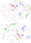 |
Fig. 1. Sky distribution of the superclusters at z ≤ 0.03 in equatorial coordinates (upper panel) and galactic coordinates (lower panel). The superclusters are marked by numbers: 1 = Perseus-Pisces Supercluster, 2 = Abell 400 supercluster, 3 = Local Supercluster, 4 = Centaurus Supercluster, 5 = Coma Supercluster 6 = Hercules supercluster, 7 = Sagittarius Supercluster, 8 = Lacerta Supercluster. The full coloured symbols are CLASSIX supercluster members, with z ≤ 0.03, while more distant members are shown by coloured open symbols. All other CLASSIX clusters at z ≤ 0.03 are shown as black open circles. The galactic band (bII = ±20°) is shown by blue dotted (dashed) lines, the region with high hydrogen column density (nH ≥ 2.5 × 1021 cm−2) is indicated by the solid blue lines, and the supergalactic band (SGZ = ±20°) by red lines. |
Properties of the superclusters in the local Universe at z ≥ 0.03 constructed with a minimal linking length, l0 = 19 Mpc.
The properties of the superclusters we list in Table 1 were determined as follows. To compare the ‘richness’ among the different SC objectively, taking the selection function into account, we determine the weighted number of members by summing the weights derived with Eq. (1). The volume of the systems was determined by taking for each member cluster a sphere with a radius of 19 Mpc, equal to the minimal linking length. The volume of the SC is then the sum of the spheres, taking the overlap into account. The mass of the clusters in the SC is the sum of the m200 values. The SC mass is estimated from the volume times the cosmic mean density times the matter overdensity ratio, RDM, of the SC. The length of the SC is determined from the largest separation of two SC members. The cluster density, nCL, is determined by the weighed number of clusters divided by the SC volume. The overdensity ratio of clusters in the SC, RCL = nCL/⟨nCL⟩ is determined with respect to the mean cluster density in Sect. 3. The dark matter overdensity is derived by means of the relation RDM = (RCL − 1)/b + 1. We used a bias factor b = 1.6, which is the average value determined for the relevant cluster sample with given lower mass limit.
The volume calculation described above is quite generous. We adopted this as the most obvious choice, because it yields an overdensity ratio of about 2, consistent with the above considerations concerning the linking length. One could in principle also argue that one should only take half the radius to the next nearest neighbour. We provide the results from such calculations with an alternative sphere radius of 10 Mpc in Table 2. We note that this results in a decrease of the estimated SC mass by only 13–23% (27% in the case of the Local SC).
4.2. Supercluster multiplicity function
The multiplicity function of SC, that is their richness distribution, is an interesting statistical tool to gain some understanding of the nature of the structures. We show in Fig. 2 the multiplicity function resulting from the SC construction with a minimal linking length of 19 Mpc, relaxing the requirement of a minimum number of members. We note that the distribution shows a steep increase in the number of SC for less than five members towards low richness, while we see a long tail in the distribution with more than five members. To better understand these results, we performed simulations of spatially random distributions of clusters with the same study volume and total number and subjected them to the same SC construction process. We repeated these simulations 1000 times and compare the mean results of these to the observations in Fig. 2. At the low richness end (NCL < 5) the random distribution reproduces the observations quite well. This implies that the steep increase towards low richness can be produced by shot noise. However, in the high richness tail the simulated SC are much less frequent than the observed ones, underlining the conclusion that these structures are especially interesting.
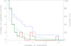 |
Fig. 2. Supercluster multiplicity function found from observations (red). The cumulative fraction of CLASSIX clusters in superclusters as a function of the number of members is shown in blue (with corresponding axis on the right). The multiplicity function for a simulated random distribution of clusters is shown in green and the corresponding fraction of clusters in superclusters as green dashed line. |
4.3. The Local Supercluster with the Virgo cluster
The structure found including the Virgo cluster, listed in Table 3, is the Local SC (de Vaucouleurs 1953, 1956, 1958). It contains only one galaxy cluster, Virgo, and several smaller galaxy groups. If we would have applied the same strict criteria, that we applied to the other superclusters, the Local SC would not have been included. We considered the Virgo cluster as three separate dynamical units, the X-ray halos around the giant elliptical galaxies M87, M86 and M49, which can be distinguished in the RASS. Among these X-ray halos, M49 falls (with its luminosity of LX ∼ 3 × 1041 erg s−1) below the sample luminosity limit and is thus excluded. The halos of M87 and M86 overlap on the sky, but one can model the X-ray surface brightness distribution with two distinct halos (Böhringer et al. 1994). Also in redshift space the two halos can be distinguished (e.g., Binggeli et al. 1987). For other systems we considered different components only if they do not overlap on the sky in the RASS. Allowing for this exception for the nearby Virgo cluster provided us with five X-ray halo members for the Local SC, making it part of the SC sample.
Groups and clusters which are members of the Local SC.
In addition, inspecting the X-ray luminosities of the five objects of the Local SC, we find that three of them have a low luminosity within a factor of two of the luminosity limit and the fourth one is only slightly more luminous. Therefore the only massive object in this structure is the main body of the Virgo cluster formed by the halo of M87. If we would have set the lower luminosity limit to ≥2 × 1042 erg s−1, the only two members left would have been M87 and NGC4636. We show in Fig. A.1 the mean luminosity limit as a function of redshift. One notes that a luminosity limit LX > 2 × 1042 erg s−1 effectively applies for all systems with redshifts z ≥ 0.0203. Thus again the Local SC would not have been included if it would not be so close. But we had a strong interest to include this well known SC in the description of the local cosmography of our Universe.
Figure 3 shows the three-dimensional configuration of the group of clusters. The two components of the Virgo cluster and NGC4636 form a tight group as well as the pair consisting of NGC5813 and NGC5846, while the two associations have a separation of about 17 Mpc, close to the linking length. Further properties of this SC are given in Tables 1 and 2, with an estimated mass of about 1.9 − 2.5 × 10¹⁵ M⊙.
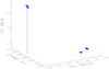 |
Fig. 3. Three-dimensional representation of the Local SC. The four objects in the lower right are the Virgo cluster, with M87, M86 and M49 as well as NGC4636. M49 is marked with an open symbol because its X-ray luminosity is below the adopted luminosity limit. |
4.4. The Centaurus Supercluster
The Centaurus SC is found with ten members whose properties are listed in Table 4. The Centaurus cluster, A3526, is by far the most massive object. One galaxy group, NGC 5090/5091 is located in the ZoA at bII ∼ 18.1°. Figure 4 shows a three-dimensional representation of the SC and its location with respect to the Local SC. The Centaurus SC is mostly oriented along the Supergalactic plane. Its has a length of about 37.1 Mpc with an extension in the SGZ direction of only about 15.2 Mpc. The estimated mass is about 4.5 − 5.6 × 10¹⁵ M⊙. It is located close to the Local SC. A linking length of 20.3 instead of 19 Mpc would merge the two superclusters through the systems RXCJ1315.3-1623 and RXCJ1501.1+0141.
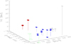 |
Fig. 4. Three-dimensional representation of the Centaurus SC (blue circles) and the Local SC (red squares). The open green squares show (from left to right) the Norma, Antlia and Hydra clusters. Other CLASSIX clusters in this volume not associated with the two SC are shown as open black circles. |
Groups and clusters which are members of the Centaurus SC.
In Fig. 5 we show three projections of the Centaurus SC in supergalactic coordinates. In this and similarly for the following figures we indicate the estimated cluster masses by the size of the symbols, with a diameter scaling with the cube root of the estimated mass. Five of the more massive members are marked in the image. The dominant Centaurus cluster sits on one side of the SC. In Fig. 4 it appears on the left (low values of SGY) together with the group NGC5090/5091 (which has the lowest SGY coordinate). The second most massive system in the SC is the group NGC 5044, with an estimated mass, m200, of about 1.08 × 10¹⁴ M⊙. The other SC members have estimated masses below 6 × 10¹³ M⊙. RXCJ1349.3-3018, A3574E, includes an X-ray bright AGN, the X-ray emission of which was subtracted in this analysis, as further explained in the Appendix.
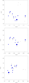 |
Fig. 5. Centaurus supercluster in three projections in Supergalactic coordinates. The SC members are shown as filled blue circles, while other CLASSIX clusters in this volume are marked by open circles. The size of the symbols is proportional to the cube root of the mass of the clusters as explained in the text. Several prominent clusters are marked. 1: Centaurus cluster, A3526, 2: NGC 5044 group, 3: AS 753, 4: A 3574 West, 5: A 3574 East. |
In the literature this structure is often described as part of the Hydra-Centaurus SC. With our recipe to construct the nearby SC, the Hydra cluster, A1060, fails to be merged with the Centaurus SC by a large margin. Similarly, the other two prominent clusters in this region, Antlia and Norma (A3627), are too distant to be linked. For the Hydra, Norma and Antlia clusters we find a distance to the nearest Centaurus SC member of 27.2, 35.1 and 22.9 Mpc, respectively, while the linking length with the weighting for the specific location turns out to be, 19, 20.3 and 19 Mpc. We discuss this further below, when we compare different linking schemes.
4.5. The Coma Supercluster
The Coma Supercluster, often also referred to as the Great Wall, is found with 11 group and cluster members in the volume out to z = 0.03. If we relax the boundary constraint, two more clusters are associated to this SC at redhifts z = 0.03 − 0.0322 as shown in Table 5. The two most prominent members of the Coma SC are the Coma cluster and A1367. All other groups and clusters have estimated masses below 1.5 × 10¹⁴ M⊙.
Groups and clusters which are members of the Coma SC.
Figure 6 displays a three-dimensional representation of the Coma SC. This structure has a slightly larger extent in the SGZ direction of 55.4 (65.3) Mpc compared to the SGX and SGY directions with an extent of 50.2 (61.8) and 38.0 (52.4) Mpc, respectively, where the number in brackets refer to the structure including the two clusters at z > 0.03. Compared to the Perseus-Pisces and Centaurus SC it is oriented much more in a perpendicular direction to the Supergalatic plane. The total length of the Coma SC is 64.8 (78) Mpc. It is thus the third largest supercluster, also in mass, next to the Perseus-Pisces and Hercules SC.
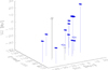 |
Fig. 6. Three-dimensional representation of the Coma SC in Supergalactic coordinates. The members of the Coma SC are shown as full blue circles, the Coma cluster is marked by a larger symbol and the two clusters at z > 0.03 are shown as open squares. All other CLASSIX clusters in the volume are shown as black open circles. |
A display of the Coma SC in three projections in Supergalactic coordinates is given by Fig. 7. The five most prominent members of the Coma SC are identified. We note that the Coma cluster and NGC 522 (RXCJ1334.3+3441) are located at positive SGZ coordinates and are separated from most other groups and clusters in the SC. NGC 522 (RXCJ1334.3+3441) is also the object furthest to the east in the sky. The two clusters with z > 0.03 have the most negative SGZ coordinates.
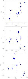 |
Fig. 7. Coma Supercluster in Supergalactic coordinates in three projections. Members of the structure are shown as filled blue circles, where the size of the symbol reflects the estimated mass of the cluster. The two clusters at z > 0.03 are shown as blue squares. All other clusters are marked by black open circles. The most massive members of the Coma supercluster are identified by numbers: 1: Coma, 2: A 1367, 3: MKW4, 4: NGC 410, 5: NGC 4325, 6: A1177, 7: A 1185. |
4.6. The Hercules Supercluster
The SC with the members shown in Table 6 consists of ten groups and poor clusters. The SC is located more than 60 Mpc above the Supergalactic plane (Figs. 8, and 9). It is part of a larger structure with its major parts outside the radius of z = 0.03. The core of this larger structure is the classical Hercules SC, with the members A2147, A2151, A2152 (e.g., Shapley 1932; Abell 1961; Tarenghi et al. 1979, 1980; Giovanelli et al. 1997). Abell (1961) considered the former three clusters together with A2162, A2197 and A2199 as one supergalactic system (‘second order cluster’). Barmby & Huchra (1998) included further clusters, A2107, A2063 and A2052 as possible members of the SC. Apart from A2197 which lies at the boundary of our study region all these clusters are located at z > 0.03. What we observe in our study-volume is just the extension of this much more massive structure, that is linked together if we extend the friends-of-friends analysis with our recipe beyond z = 0.03. We describe the entire structure in more detail in a subsequent publication and concentrate here on our study volume.
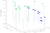 |
Fig. 8. Three-dimensional representation of Hercules supercluster in Supergalactic coordinates. The members of the SC at z ≤ 0.03 are shown as solid blue circles, some of the structure beyond with open green circles. Other CLASSIX clusters in the study volume are marked by open black circles. |
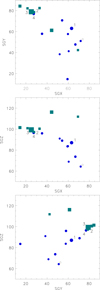 |
Fig. 9. Hercules supercluster in Supergalactic coordinates in three projections. The size of the symbols indicates their mass. Supercluster members with z ≤ 0.03 are shown as solid blue circles, those at z > 0.03 with blue squares, and other CLASSIX clusters in this volume with open black circles. The clusters with numbers are: 1 = NGC 6338, 2 = A2197W, 3 = A2199, 4 = A2197E. |
Groups and clusters which are members of the Hercules SC at z ≤ 0.03.
The part of the Hercules SC inside the study region contains mostly less massive systems with masses below 1014 M⊙, except for RXCJ1715.3+5724 (NGC 6338) with an estimated mass of about m200 = 1.7 × 10¹⁴ M⊙. The next massive object is RXCJ1629.6+4049 (A2197E) through which this structure connects to the classical Hercules SC. Figure 8 shows the locations of the Hercules SC members at z ≤ 0.03 and a few clusters at higher redshift including the concentration A2197E, 2197W and A2199.
NGC 6338 has been observed with Chandra and XMM-Newton and studied in detail by Pandage et al. (2012) and O’Sullivan et al. (2019). It is found to be an interesting merger of a smaller group with the main system. NGC 6338 also hosts interesting radio lobe cavities. The temperature outside the core is about 2–3 keV (O’Sullivan et al. 2019).
4.7. The Sagittarius Supercluster
Six objects in the southern sky, as listed in Table 7, are linked together to a supercluster in the constellation of Sagittarius. We have not found a previous description of this structure and thus refer to it as the Sagittarius SC. All members have estimated masses below m200 = 7 × 10¹³ M⊙. The most massive one is the group around the galaxy ESO 460 - G004 (m200 = 6.5 × 10¹³ M⊙). Figure 10 provides a three-dimensional representation of the structure. The SC has a length of 33.8 Mpc and an estimated mass of 4.3 − 5.5 × 10¹⁵ M⊙.
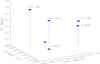 |
Fig. 10. Three-dimensional representation of distribution of the members of the Sagittarius SC in Supergalactic coordinates. The galaxy groups are designated by the names of their central galaxies. |
Groups and clusters which are members of the Sagittarius SC.
4.8. The Lacerta Supercluster
In Supergalactic coordinates the Lacerta SC is located about 40 to 50 Mpc above the Perseus-Pisces SC. It contains six members all of which have estimated masses bellow m200 = 1.1 × 10¹⁴ M⊙, as listed in Table 8. The SC is entirely located in the ZoA. Figure 11 provides a three-dimensional view on the SC. One notes the close pair of the two groups, UGC 12491 (CIZA2318.6+4257) and NGC 7618, which have almost the same redshift. They both have been found in Chandra observations to be interesting interacting systems with sloshing cold fronts (Kraft et al. 2006).
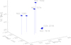 |
Fig. 11. Three-dimensional representation the Lacerta SC in Supergalactic coordinates. The galaxy groups are designated by the names of their central galaxies, except for one unmarked object, which contains the giant elliptical UC 12064 slightly off-centre. |
Groups and clusters which are members of the Lacerta SC.
The SC has a length of 19.9 Mpc and an estimated mass of 3.6 − 4.3 × 10¹⁵ M⊙. Apart from the Local SC it is the smallest of the SC in the study volume. We show below that it merges with the Perseus-Pisces SC with linking schemes at a higher X-ray luminosity limit.
4.9. Overview
Figure 12 provides an overview of all the structures in the study volume in a three-dimensional representation. Among the two panels, the lower one provides a slightly better separation of the SC. While in total we found 146 groups and clusters with Lx ≥ 1042 erg s−1 at z ≤ 0.03; 75 of these are part of superclusters (a fraction of 51%). This result is similar to that found for superclusters in the entire REFLEX survey by Chon & Böhringer (2013). If we compare the volumes based on the values in Table 1, however, we find that the SC occupy only ∼14% of the study volume at z ≤ 0.03. Using the alternative volume calculation with 10 Mpc radius of Table 2, the volume fraction is only about 1.8%.
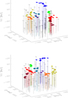 |
Fig. 12. Three-dimensional representation of all supercluster found within z ≤ 0.03 with at least five members and a minimum linking length of l0 = 19 Mpc. The structures marked in colour are: red = Perseus-Pisces SC, red-brown = A400 SC, violet = Local SC, orange = Centaurus SC, siena = Coma SC, dark blue = Hercules SC, turquoise = Sagittarius SC, light green = Lacerta SC. Non-supercluster members are shown as black open circles. |
Inspecting the cluster and SC distribution in the plot, we note two clear asymmetries. In equatorial coordinates we find 86 clusters in the northern compared to 60 in the southern sky, which is an overabundance by about 1.5σ in the north. But looking at the number of cluster which are members of SC we find a more than 6σ difference, 57 compared to 18, respectively. Thus there are clearly more SC in the northern sky, including the Perseus-Pisces SC, most of the A400, the Local, the Coma, the Hercules, and the Lacerta SC, compared to Centaurus and Sagittarius SC in the southern sky (see also Fig. 1). The other inhomogeneity concerns the SC distribution with respect to the Supergalactic SGZ coordinate. There is no significant difference in the number above and below SGZ = 0: 67/79 for all clusters, 39/36 for clusters in SC. But there is a striking difference if we compare the number of clusters at SGZ ≥ 50 Mpc with those at SGZ ≤ −50 Mpc, which is 29/18 for all clusters and 16/0 for clusters in SC. Thus we find no SC in the volume of z ≤ 0.03 and SGZ ≤ −50 Mpc. We also note the strong segregation towards the Supergalactic plane, that we studied in detail in Böhringer et al. (2021a). Among the eight supercluster, the four major ones, Perseus-Pisces, Centaurus, Coma, and Hercules SC, are clearly recognised as the largest structures.
5. Discussion
5.1. Effect of the lower luminosity limit for member clusters
We have constructed the SC described above with groups and clusters of galaxies with a low X-ray luminosity limit, much lower than what was typically used in the past. The advantage of this procedure is that we can base the cluster density mapping on a sufficiently high cluster density, which is less subject to shot noise. But it also raises the interesting question, in how much the SC found depend on this lower luminosity limit. To test this, we conducted the following study. We repeated the SC construction with a series of schemes involving an increasing X-ray luminosity limit. By increasing this limit, we are thinning out the cluster density. To compensate for this, we increased the linking length accordingly. This was done using the following equation,
 (2)
(2)
where l0 is the nominal (minimal) linking length defined in Sect. 3,  is the new nominal linking length. nCL(LX0) is the cluster density as a function of lower luminosity limit, where LX0 and
  are the nominal and new lower X-ray luminosity limits. For this study we varied
  over an order of magnitude in eight steps including the linking schemes listed in Table 9, which gives the values of the lower luminosity limit,
  , and the nominal linking length,
  , for each step. With each step the density mapping gets noisier. To provide a feeling for this effect, we give in the forth row, labelled NCL, the number of clusters at z ≤ 0.03 above
  . Up to step four we only consider SC with at least five members, as done above. From step 5 on we also consider structures with four members, since the statistics gets considerably poorer. In this exercise we are including only groups and clusters at redshifts z ≤ 0.03.
Supercluster membership as a function of the lower X-ray luminosity limit,  .
.
The smaller structures do not survive all the steps. The Local SC gets merged with the Centaurus SC already in step 2, similar to the behaviour we saw in Sect. 4.3. The A400 SC, which does not contain many massive clusters, is not recovered in step 3. The Sagittarius SC is lost in step 4 and the Lacerta SC survives with four members up to step 4 and merges in step 5 with the Perseus-Pisces SC. Only the larger SC survive till the highest luminosity limit, except for the Hercules supercluster (lost in step 4). The latter has its core outside the considered redshift range and it would only survive if we had included also this part. The fact that the smaller structures are not traced well if we lower the statistics is not surprising, since the density mapping is just not fine enough to recognise them.
In Figs. 13–15 we give an impression how the larger structures survive the increase of the X-ray luminosity limit. In these figures the solid circles and squares show the structure recovered at the lowest and the large open circles the structure found at the highest X-ray luminosity limit. For the Perseus-Pisces SC we note in Fig. 13 that the main chain of clusters of this SC is found over the complete luminosity limit range. However, while a small ensemble of galaxy groups found at the lowest  in the west of the SC is lost at higher
  , the Lacerta SC with four clusters is linked to the Perseus-Pisces SC on the western side in step 5.
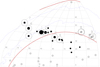 |
Fig. 13. Cluster members of the Perseus-Pisces SC for different linking schemes. The solid black points show the SC members found for scheme 1 and the large open circles show the members found for scheme 8. The object marked by an open square is first found with scheme 5. Some prominent clusters are marked: 1 = Perseus, 2 = AWM7, 3 = A262, 4 = NGC 507, 5 = NGC 383, 6 = 3C129, 7 = UGC 12655, 8 = double cluster RXCJ2318.6+4257, RXCJ2319.7+4521, 9 = NGC7242. The blue lines constrain the region of high interstellar absorption, the red lines show galactic latitudes bII ± 20°. |
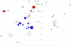 |
Fig. 14. Cluster members of the Centaurus SC and the Local SC for different linking schemes. The solid circles and the red squares show the Centaurus and Virgo superclusters found with scheme 1, the crosses mark those found with scheme 2 and the large open circles mark those found with scheme 8. The open squares show two clusters linked at intermediate schemes 3 and 5, respectively. Some prominent clusters are marked: 1 = Centaurus, 2 = NGC 5044, 3 = M87, 4 = Hydra (A1060), 5 = Antlia, 6 = HCG 62, 7 = A3581, 8 = Norma (A3627), 9 = RXCJ1324.7-5736. |
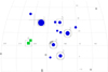 |
Fig. 15. Cluster members of the Coma SC for different linking schemes. The solid blue circles describe the structure found with scheme 1, while the large open squares and open circles mark the structure found with schemes 7 and 8, respectively. The green squares show the clusters linked with scheme 3. Some prominent clusters are marked: 1 = Coma cluster, 2 = A 1367, 3 = MKW4, 4 = NGC 4325, 5 = NGC 410, 6 = NGC 5171. |
For the Centaurus cluster (Fig. 14) the first step brings a significant increase, where the Local SC is linked with two members and also Hydra, Antlia and another cluster are added. At the highest luminosity limit also the Norma cluster and another luminous cluster in the ZoA gets linked. For the Coma SC, shown in Fig. 15, we note less changes. In step 3 two groups around the galaxies NGC 5129 and NGC 5171 get linked and then the overall structure remains with fewer members until the highest luminosity limit.
Thus we find that the construction of SC with the FoF scheme applied here is robust and not much sensitive to the details of the linking parameters for the given overdensity selection. There is some change in the linking of different small extensions and an overall trend that the structures become slightly larger with increasing luminosity limit. But the main structures stay the same. Another very important fact is that no new structure appeared in this process that would have been missed in the first analysis.
It is interesting to note that the linking of the clusters at higher  finds the Hydra-Centaurus SC as one unit, which is similar to most descriptions in the literature. Similarly interesting is the merging of the Perseus-Pisces and Lacerta SC at higher
  . In this case the inclusion of the Lacerta members indicates an upturn of the Perseus-Pisces SC on the western side. Such an upturn is prominently seen in the galaxy distribution if radio observations in HI are included in the redshift surveys. Kraan-Korteweg et al. (2018) show in their Fig. 10 the galaxy distribution around the Perseus-Pisces SC and one can clearly note the pronounced filament of the SC. Around lII ∼ 115° and bii ∼ −30° this galaxy filament turns northward in Galactic coordinates and crosses the equatorial plane around lii = 90°. The ensemble of galaxy groups of the Lacerta SC falls roughly into the middle of this upturning filament and thus also traces this SC extension.
5.2. Comparison to previous studies of superclusters of clusters
Of the eight systems in our sample of SC, the five most prominent structures have been previously known and are, for example, described in the review by Oort (1983). For these SC we can compare the size of the systems quoted in the review with our findings. The size of the Local SC was given as ∼28.6 Mpc (18.5 Mpc), for the Perseus SC 54 Mpc (116 Mpc), for the Coma SC 65–114 Mpc (78 Mpc), for Hydra-Centaurus SC 64 Mpc (37 Mpc), and for the Hercules SC 100 Mpc (140 Mpc), where the numbers in brackets are our results from Table 1. The sizes from Oort (1983) were converted from a scaling with a Hubble constant of H0 = 50 km s−1 Mpc−1 to the value of 70 km s−1 Mpc−1 used here. The largest differences are for the Perseus SC, where we now include an extension through the ZoA, and for the Centaurus SC where we have not included the complex around the Hydra cluster as discussed in the previous section. Already Joeveer & Einasto (1978) found that the Perseus-Pisces SC is the most prominent superstructure in the nearby Universe. They assigned a mass of about  to this SC which is similar to our result. This earlier mass is a little smaller as the extension across the ZoA was not included. Overall these major structures have been recognised in a similar way in many different studies, some of which were already mentioned above in the corresponding sections of the SC, which shows that their recognition in the galaxy cluster distribution as distinct superstructures is robust.
5.3. Comparison to other studies of the large-scale structure
Our results can also be compared to methods of characterising the cosmic large-scale structure other than those using galaxy clusters, such as the cosmic flow analysis based on galaxy peculiar velocities, the study of the galaxy density distribution, and various ways of geometrical characterisations of the cosmic web. The use of galaxy peculiar velocities to trace the matter distribution in the Universe is a sensitive method, but restricted to the local Universe in the volume in which peculiar velocities can be determined with sufficient precision. That our results are also confined to the nearby Universe in only a slightly larger volume, makes a comparison with the results from a cosmic flow analysis, like those of the group of Tully, interesting. In Fig. 1 of Tully et al. (2019) the four major nearby mass concentration labelled as Virgo and Great Attractor, Coma, Perseus-Pisces, and Hercules, are the same five major structures we found here. Starting from our local position we find that the Local SC is closely linked to the Centaurus or Hydra-Centaurus complex. This is what Tully et al. (2014) found in their streaming analysis which links the Local SC, to the Great Attractor in the Hydra-Centaurus region. All of this together with the Norma cluster is combined into the Laniakea SC. In a stricter mathematical approach to segment the major structure in the local cosmic flows by Dupuy et al. (2019, 2020) the authors isolate the structures into basins of attraction by following individual streamlines to common destinations. They used the Constrained Local UniversE Simulations (CLUES; Yepes et al. 2009; Gottlöber et al. 2010) for their study and identified as major attractors the Laniakea SC (volume = 5 × 10⁵ (Mpc h−1)3), Coma SC (volume = 1 × 10⁶ (Mpc h−1)3), and Perseus-Pisces SC (volume = 7 × 10⁵ (Mpc h−1)3). The typical mass of their basins of attraction is about = 5×10¹⁶ M⊙ h−1. The volumes are about three to five times larger than the values we find and the typical mass is about two to three times higher than that for the larger structures in our sample. This difference is due to the different definitions of the structures. While we only consider the overdense regions of the SC, the basins of attraction include the complete surroundings of the SC. Accounting for this fact by considering the filling factors of our SC, the results become quite similar.
Most of the more recent studies of SC in the galaxy distribution are based on the SDSS or the 2degree Field Galaxy Redshift Survey (2dFGRS) at redshifts outside our study volume. Therefore we can only make a statistical comparison. Einasto et al. (2007a,b) have identified SC in the 2dFGRS with a density field method, finding large structures in the galaxy density distribution smoothed with an Epanechnikov kernel of radius 8 h−1 Mpc as overdensities. The richest of these SC have typical radii of about 50 to slightly over 100 h−1 Mpc. They also analyse cosmological simulations, the Millennium run galaxy catalogue by Croton et al. (2006), for comparison and find SC with similar sizes. These structures can well be identified with the type of SC we find. Liivamaegi et al. (2012) identified and studied superclusters in a similar way in the SDSS with the density field method. For a plausible density threshold D ∼ 5 for the selection of SC they find the largest SC to have diameters of 100 − 200 h−1 Mpc. With the extended percolation analysis Einasto et al. (2018, 2019, 2021) detected SC in the galaxy distribution of the SDSS with a similar density threshold of D = 5 as used by Liivamaegi et al. (2012) and find that the size function is cut off at diameters slightly larger than 100 h−1 Mpc. Einasto et al. (2016) have analysed the region of the Sloan Great Wall with a similar recipe as Liivamaegi et al. (2012). This is one of the largest structures found with an estimated length of about  Mpc. In their analysis the Sloan Great Wall breaks up into two larger and three smaller SC. The two larger SC have masses in the range
  . We therefore note that these studies of SC in the galaxy distribution, which cover a much larger cosmic volume, do not unvail much larger SC than what we found in the nearby Universe.
An overview on different geometrical ways to characterise the cosmic web is for example given by Cautun et al. (2014) (see also Liebeskind et al. 2018). They identify structures with different morphologies in the cosmic web: clusters, filaments, sheets, and voids. They find that filaments dominate the cosmic web at least since z ∼ 2, carrying about 50% of the total mass at present. The filaments have a fractal distributions over a range of scales and most of the mass is carried by the most massive filaments. The largest filaments have an extent over 100 h−1 Mpc and connect several clusters in a linear configuration. Therefore we can identify the superclusters we find with the massive filaments of the geometrical analysis. We thus find good agreement, with the minor exception, that we would not stress that these structures are generally linear chains of clusters, which we find in such a pronounced way particularly for the Perseus-Pisces SC.
5.4. Luminosity distribution of Supercluster members
In our previous study on the Perseus-Pisces and A400 SC, we found a hint that the clusters in SC are on average more X-ray luminous than in the field. This was found at high significance in the study of all the superstes-clusters in the REFLEX sample and in simulations by Chon & Böhringer (2013) and Chon et al. (2014). Figure 16 shows the luminosity distribution for the clusters at z ≤ 0.03 inside and outside the superclusters. There are more very luminous clusters in SC, but at the low luminosity end we see also more small systems in the SC. The mean X-ray luminosity of all clusters is LX = 2.0 × 1043 erg s−1 for the field and LX = 2.5 × 1043 erg s−1 for the SC members. The difference is caused by the two most luminous clusters. We get a somewhat clearer picture of the difference of the luminosity distribution, if we concentrate on clusters at higher luminosity, with, for example, a lower luminosity limit of LX = 0.5 × 1043 erg s−1. This is shown in Fig. 17 for the comparison of members in all SC to those in the field (in the left panel) and for members of the four largest SC compared to the field (in the right panel). The hint to a difference becomes clearer for the four largest SC, while the four smaller SC rather dilute this difference. It is also interesting that the SC contain also a large number of small systems, which weaken the overall trend. Kolmogorov-Smirnov statistical tests show, however, that these results are not highly significant and better statistics is needed to firmly establish these findings.
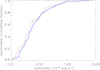 |
Fig. 16. Cumulative normalised X-ray luminosity distribution of clusters in the eight superclusters (red dashed line) compared to the distribution for clusters in the field (blue solid line). |
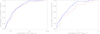 |
Fig. 17. Cumulative normalised X-ray luminosity distribution of clusters in the eight superclusters (red dashed line) compared to the distribution for clusters in the field (blue solid line) with a lower X-ray luminosity limit of 0.5 × 1043 erg s−1. The data in the left panel include all eight superclusters, those in the right panel only the four large superclusters. |
6. Summary and conclusion
We searched for large-scale structures in the matter distribution in the nearby Universe at z ≤ 0.03 with overdensity ratios of about two by means of the distribution of X-ray luminous galaxy groups and clusters with an estimated mass larger than about m200 = 2.1 × 10¹³ M⊙. In total we found eight superclusters with at least five group or cluster members. Four of these are smaller with estimated masses in the range of 2 − 7 × 10¹⁵ M⊙. They are the Local, the A400, the Sagittarius and the Lacerta SC. The latter two are structures which have not been described as such. These smaller structures are only found by including less massive groups of galaxies with low X-ray luminosities of a few 1042 erg s−1.
The other four SC are well known, prominent mass concentrations, the Perseus-Pisces SC, the Centaurus SC (sometimes identified as Great Attractor), the Coma SC with the massive Coma cluster, and the low redshift part of the Hercules SC. These have estimated masses in the range 0.5 − 2.2 × 10¹⁶ M⊙. The largest structure is clearly the Perseus-Pisces SC. We showed that variations of the structure construction schemes robustly recover approximately the same prominent structures and no other structures appeared for a wide range of construction parameters. These major structures are consistent with the results from the analysis of cosmic flows from galaxy peculiar velocities (e.g., Tully et al. 2019) and also with other large-scale structure studies.
We provided catalogues and maps of all the member groups and clusters in the Appendix and verified that all of them show significantly extended X-ray emission in the ROSAT All-Sky Survey. In total 51% of all the X-ray luminous groups and clusters at z ≤ 0.03 are members of these SC. This characterisation of the large-scale environment of superclusters in the local Universe should be interesting for studies of the environmental dependence of the properties of different astronomical objects. It is also important for a better understanding of our local reference system from which we perform precision cosmology observations.
The values for the interstellar hydrogen column density are taken from the 21 cm survey of Dickey & Lockman (1990). We have compared the interstellar hydrogen column density compilation by Dickey & Lockman (1990) with the more recent data set of the Bonn-Leiden-Argentine 21 cm survey (Kalberla et al. 2005) and found that the differences relevant for us are of the order of at most one percent. Because our survey has been constructed with a flux cut based on the Dickey & Lockman results, we keep the older hydrogen column density values for consistency reasons.
r500 is the radius where the average mass density inside reaches a value of 500 times the critical density of the Universe at the epoch of observation.
available at http://archive.eso.org/dss/dss
Acknowledgments
We thank the referee, Jaan Einasto, for very helpful comments and suggestions. We acknowledge support of the Deutsche Forschungsgemeinschaft through the Munich Excellence Cluster ‘Universe’. G.C. acknowledges support by the DLR under grant no. 50 OR 1905.
References
- Abell, G. O. 1958, ApJS, 3, 211 [NASA ADS] [CrossRef] [Google Scholar]
- Abell, G. O. 1961, AJ, 66, 607 [CrossRef] [Google Scholar]
- Abell, G. O., Corvin, H. G., & Olowin, R. P. 1989, ApJS, 70, 1 [NASA ADS] [CrossRef] [Google Scholar]
- Alpaslan, M., Driver, S., Robotham, A. S. G., et al. 2015, MNRAS, 451, 3249 [Google Scholar]
- Bahcall, N. 1988, ARA&A, 26, 631 [NASA ADS] [CrossRef] [Google Scholar]
- Bahcall, N. A., & Soneira, R. M. 1983, ApJ, 270, 20 [NASA ADS] [CrossRef] [Google Scholar]
- Bahcall, N. A., & Soneira, R. M. 1984, ApJ, 277, 27 [NASA ADS] [CrossRef] [Google Scholar]
- Balaguera-Antolinez, A., Sanchez, A., Böhringer, H., et al. 2011, MNRAS, 413, 386 [NASA ADS] [CrossRef] [Google Scholar]
- Balaguera-Antolinez, A., Sanchez, A., Böhringer, H., et al. 2012, MNRAS, 425, 2244 [NASA ADS] [CrossRef] [Google Scholar]
- Bardeen, J. M., Bond, J. R., Kaiser, N., et al. 1986, ApJ, 304, 15 [NASA ADS] [CrossRef] [Google Scholar]
- Barmby, P., & Huchra, J. P. 1998, AJ, 115, 6 [NASA ADS] [CrossRef] [Google Scholar]
- Basilakos, S., Plionis, M., & Rowan-Robinson, M. 2001, MNRAS, 323, 47 [Google Scholar]
- Batuski, D. J., & Burns, J. O. 1985, ApJ, 299, 5 [NASA ADS] [CrossRef] [Google Scholar]
- Binggeli, B., Tammann, G. A., & Sandage, A. 1987, AJ, 94, 251 [Google Scholar]
- Böhringer, H., Briel, U. G., Schwarz, R. A., et al. 1994, Nature, 368, 828 [CrossRef] [Google Scholar]
- Böhringer, H., Schuecker, P., Guzzo, L., et al. 2004, A&A, 425, 367 [NASA ADS] [CrossRef] [EDP Sciences] [Google Scholar]
- Böhringer, H., Chon, G., Collins, C. A., et al. 2013, A&A, 555, A30 [Google Scholar]
- Böhringer, H., Chon, G., Collins, C. A., et al. 2014, A&A, 570, A31 [NASA ADS] [CrossRef] [EDP Sciences] [Google Scholar]
- Böhringer, H., Chon, G., Bristow, M., et al. 2015, A&A, 574, A26 [NASA ADS] [CrossRef] [EDP Sciences] [Google Scholar]
- Böhringer, H., Chon, G., Retzlaff, J., et al. 2017, AJ, 153, 220 [Google Scholar]
- Böhringer, H., Chon, G., & Collins, C. A. 2020, A&A, 633, 19 [Google Scholar]
- Böhringer, H., Chon, G., & Trümper, J. 2021a, A&A, 651, A15 [NASA ADS] [CrossRef] [EDP Sciences] [Google Scholar]
- Böhringer, H., Chon, G., & Trümper, J. 2021b, A&A, 651, A16 [NASA ADS] [CrossRef] [EDP Sciences] [Google Scholar]
- Cautun, M., van de Weygaert, R., Jones, B. J. T., et al. 2014, MNRAS, 441, 2923 [CrossRef] [Google Scholar]
- Chamaraux, P., Cayatte, V., Balkoski, C., et al. 1990, A&A, 229, 340 [Google Scholar]
- Chincarini, G. L., Giovanelli, R., & Haynes, M. P. 1983, A&A, 121, 5 [Google Scholar]
- Chon, G., & Böhringer, H. 2013, MNRAS, 429, 3272 [NASA ADS] [CrossRef] [Google Scholar]
- Chon, G., Böhringer, H., Collins, C. A., et al. 2014, A&A, 567, A144 [NASA ADS] [CrossRef] [EDP Sciences] [Google Scholar]
- Chon, G., Böhringer, H., & Zaroubi, S. 2015, A&A, 575, L14 [NASA ADS] [CrossRef] [EDP Sciences] [Google Scholar]
- Churazov, E., Khabibullin, I., Lyskova, N., et al. 2021, A&A, 651, A41 [NASA ADS] [CrossRef] [EDP Sciences] [Google Scholar]
- Collins, C. A., Guzzo, L., Böhringer, H., et al. 2000, MNRAS, 319, 939 [Google Scholar]
- Costa-Duarte, M. V., Sodre, L., Jr., & Durret, F. 2011, MNRAS, 411, 1716 [NASA ADS] [CrossRef] [Google Scholar]
- Courtois, H. M., Pomàrede, D., Tully, R. B., et al. 2013, AJ, 146, 69 [NASA ADS] [CrossRef] [Google Scholar]
- Crook, A. C., Huchra, J. P., Martimbeau, N., et al. 2007, ApJ, 655, 790 [Google Scholar]
- Croton, D. J., Springel, V., White, S. D. M., et al. 2006, MNRAS, 365, 11 [Google Scholar]
- de Vaucouleurs, G. 1953, AJ, 58, 30 [Google Scholar]
- de Vaucouleurs, G. 1956, Vistas Astron., 2, 1584 [NASA ADS] [CrossRef] [Google Scholar]
- de Vaucouleurs, G. 1958, ApJ, 63, 223 [Google Scholar]
- de Vaucouleurs, G., de Vaucouleurs, A., Jr., Corwin H. G., et al. 1991, The Third Catalogue of Bright Galaxies (RC3) (Austin: University of Texas Press) [Google Scholar]
- Dickey, J. M., & Lockman, F. J. 1990, ARA&A, 28, 215 [Google Scholar]
- Dupuy, A., Courtois, H. M., Dupont, F., et al. 2019, MNRAS, 489, L1 [CrossRef] [Google Scholar]
- Dupuy, A., Courtois, H. M., Libeskind, N. I., et al. 2020, MNRAS, 493, 3513 [NASA ADS] [CrossRef] [Google Scholar]
- Einasto, M., Tago, E., Jaaniste, J., et al. 1997, A&AS, 123, 119 [NASA ADS] [CrossRef] [EDP Sciences] [Google Scholar]
- Einasto, M., Einasto, J., Tago, E., et al. 2001, AJ, 122, 2222 [NASA ADS] [CrossRef] [Google Scholar]
- Einasto, J., Hütsi, G., Einasto, M., et al. 2003a, A&A, 405, 425 [NASA ADS] [CrossRef] [EDP Sciences] [Google Scholar]
- Einasto, J., Einasto, M., Hütsi, G., et al. 2003b, A&A, 410, 425 [NASA ADS] [CrossRef] [EDP Sciences] [Google Scholar]
- Einasto, J., Einasto, M., Saar, E., et al. 2006, A&A, 459, 1 [Google Scholar]
- Einasto, J., Einasto, M., Saar, E., et al. 2007a, A&A, 462, 397 [NASA ADS] [CrossRef] [EDP Sciences] [Google Scholar]
- Einasto, J., Einasto, M., Tago, E., et al. 2007b, A&A, 462, 811 [NASA ADS] [CrossRef] [EDP Sciences] [Google Scholar]
- Einasto, M., Lietzen, H., Gramann, M., et al. 2016, A&A, 595, A70 [NASA ADS] [CrossRef] [EDP Sciences] [Google Scholar]
- Einasto, J., Suhhonenko, I., Liivamägi, L. J., et al. 2018, A&A, 616, A141 [NASA ADS] [CrossRef] [EDP Sciences] [Google Scholar]
- Einasto, J., Suhhonenko, I., Liivamägi, L. J., et al. 2019, A&A, 623, A97 [NASA ADS] [CrossRef] [EDP Sciences] [Google Scholar]
- Einasto, M., Deshev, B., Tenjes, P., et al. 2020, A&A, 641, A172 [NASA ADS] [CrossRef] [EDP Sciences] [Google Scholar]
- Einasto, J., Hütsi, G., Suhhonenko, I., et al. 2021, A&A, 647, A17 [NASA ADS] [CrossRef] [EDP Sciences] [Google Scholar]
- Giovanelli, R. 1983, in Early Evolution of the Universe and its Present Structure, eds. G. Chincarini, & G. Abell, IAU Symp., 104, 273 [NASA ADS] [CrossRef] [Google Scholar]
- Giovanelli, R., Haynes, M. P., & Chincarini, G. L. 1986, ApJ, 300, 77 [NASA ADS] [CrossRef] [Google Scholar]
- Giovanelli, R., Haynes, M. P., Herter, T., et al. 1997, AJ, 113, 53 [NASA ADS] [CrossRef] [Google Scholar]
- Giovanelli, R., Dale, D. A., Haynes, M. P., et al. 1999, ApJ, 525, 25 [NASA ADS] [CrossRef] [Google Scholar]
- Gottlöber, S., Hoofman, Y., & Yepes, G. 2010, High Performance Computing in Science and Engineering. Gaching, 2009, 309 [Google Scholar]
- Gregory, S. A., & Thompson, L. A. 1984, ApJ, 286, 422 [NASA ADS] [CrossRef] [Google Scholar]
- Gregory, S. A., Thompson, L. A., & Tifft, W. G. 1981, ApJ, 243, 411 [NASA ADS] [CrossRef] [Google Scholar]
- Guzzo, L., Schuecker, P., Böhringer, H., et al. 2009, A&A, 499, 357 [NASA ADS] [CrossRef] [EDP Sciences] [Google Scholar]
- Hauser, M. G., & Peebles, P. E. J. 1973, ApJ, 185, 757 [NASA ADS] [CrossRef] [Google Scholar]
- Henry, J. P., Gioia, I. M., Huchra, J. P., et al. 1995, ApJ, 449, 422 [NASA ADS] [CrossRef] [Google Scholar]
- Hauschildt, M. 1987, A&A, 184, 43 [Google Scholar]
- Joeveer, M., & Einasto, J. 1978, IAU Symp., 79, 241 [Google Scholar]
- Joeveer, M., Einasto, J., & Tago, E. 1978, MNRAS, 185, 357 [NASA ADS] [CrossRef] [Google Scholar]
- Kaiser, N. 1986, MNRAS, 222, 323 [Google Scholar]
- Kalberla, P. M. W., Burton, W. B., & Hartmann, D. 2005, A&A, 440, 775 [NASA ADS] [CrossRef] [EDP Sciences] [Google Scholar]
- Kerscher, M., Mecke, K., Schuecker, P., et al. 2001, A&A, 377, 1 [NASA ADS] [CrossRef] [EDP Sciences] [Google Scholar]
- Kraan-Korteweg, R. C., van Driel, W., Schröder, A. C., et al. 2018, MNRAS, 481, 1262 [NASA ADS] [CrossRef] [Google Scholar]
- Kraft, R. P., Jones, C., & Nulsen, P. E. J. 2006, ApJ, 640, 762 [NASA ADS] [CrossRef] [Google Scholar]
- Lahav, O., Santiago, B. X., Webster, A. M., et al. 2000, MNRAS, 312, 166 [NASA ADS] [CrossRef] [Google Scholar]
- Lee, G. H., Hwang, H. S., Sohn, J., et al. 2017, ApJ, 835, 280 [NASA ADS] [CrossRef] [Google Scholar]
- Liebeskind, N. I., van de Weygaert, R., Cautun, M., et al. 2018, MNRAS, 473, 1195 [NASA ADS] [CrossRef] [Google Scholar]
- Lietzen, H., Tempel, E., Heinämäki, P., et al. 2012, A&A, 545, A104 [NASA ADS] [CrossRef] [EDP Sciences] [Google Scholar]
- Liivamaegi, L. J., Tempel, E., & Saar, E. 2012, A&A, 539, A80 [NASA ADS] [CrossRef] [EDP Sciences] [Google Scholar]
- Luparello, H., Lares, M., Lambas, D. G., & Padilla, N. 2011, MNRAS, 415, 964 [Google Scholar]
- Machacek, M. E., Diab, J., Kraft, R., et al. 2011, ApJ, 743, 15 [NASA ADS] [CrossRef] [Google Scholar]
- Mahdavi, A., Böhringer, H., Geller, M. J., et al. 2000, ApJ, 534, 114 [NASA ADS] [CrossRef] [Google Scholar]
- Mo, H. J., & White, S. D. M. 1996, MNRAS, 282, 347 [Google Scholar]
- Muriel, H., Böhringer, H., & Voges, W. 1996, Int. Conf. X-ray Astronomy andAstrophyics: Röntgenstrahlung from the Universe, 601 [Google Scholar]
- Oort, J. H. 1983, ARAA, 21, 373 [NASA ADS] [CrossRef] [Google Scholar]
- O’Sullivan, E., Ponman, T. J., Kolokythas, K., et al. 2017, MNRAS, 472, 1482 [CrossRef] [Google Scholar]
- O’Sullivan, E., Schellenberger, G., Burke, D. J., et al. 2019, MNRAS, 488, 2925 [CrossRef] [Google Scholar]
- Pandage, M. B., Vagshette, N. D., David, L. P., et al. 2012, MNRAS, 421, 808 [NASA ADS] [Google Scholar]
- Park, C., Choi, Y.-Y., & Vogeley, M. S. 2007, ApJ, 658, 898 [NASA ADS] [CrossRef] [Google Scholar]
- Pratt, G. W., Croston, J. H., Arnaud, M., & Böhringer, H. 2009, A&A, 498, 361 [NASA ADS] [CrossRef] [EDP Sciences] [Google Scholar]
- Ramatsoku, M., Verheijen, M. A. W., Kraan-Korteweg, R. C., et al. 2016, MNRAS, 460, 923 [NASA ADS] [CrossRef] [Google Scholar]
- Randall, S. W., Nulsen, P. E. J., Jones, C., et al. 2015, ApJ, 805, 112 [NASA ADS] [CrossRef] [Google Scholar]
- Shapley, H. 1932, Ann. Harvard College Obs., 88, 41 [NASA ADS] [Google Scholar]
- Schuecker, P., Böhringer, H., Guzzo, L., et al. 2001, A&A, 368, 86 [NASA ADS] [CrossRef] [EDP Sciences] [Google Scholar]
- Schuecker, P., Guzzo, L., Collins, C. A., et al. 2002, MNRAS, 335, 807 [NASA ADS] [CrossRef] [Google Scholar]
- Schuecker, P., Böhringer, H., Collins, C. A., et al. 2003a, A&A, 398, 867 [NASA ADS] [CrossRef] [EDP Sciences] [Google Scholar]
- Schuecker, P., Caldwell, R. R., Böhringer, H., et al. 2003b, A&A, 402, 53 [NASA ADS] [CrossRef] [EDP Sciences] [Google Scholar]
- Sheth, R. K., & Tormen, G. 1999, MNRAS, 308, 119 [Google Scholar]
- Springel, V., White, S. D. M., Jenkins, A., et al. 2005, Nature, 435, 629 [Google Scholar]
- Tarenghi, M., Tifft, W. G., & Chincarini, G. 1979, ApJ, 234, 793 [NASA ADS] [CrossRef] [Google Scholar]
- Tarenghi, M., Chincarini, G., Rood, H. J., et al. 1980, ApJ, 235, 724 [NASA ADS] [CrossRef] [Google Scholar]
- Tinker, J. L., Robertson, B. E., & Kravtsov, A. V. 2010, ApJ, 724, 878 [NASA ADS] [CrossRef] [Google Scholar]
- Trasart-Battistani, R. 1998, A&AS, 130, 341 [NASA ADS] [CrossRef] [EDP Sciences] [Google Scholar]
- Trümper, J. 1993, Science, 260, 1769 [Google Scholar]
- Tully, R. B., Courtois, H., Hoffman, Y., et al. 2014, Nature, 531, 71 [NASA ADS] [CrossRef] [Google Scholar]
- Tully, R. B., Pomarede, D., Graziani, R., et al. 2019, ApJ, 880, 24 [NASA ADS] [CrossRef] [Google Scholar]
- van der Linden, A., Best, P. N., Kauffmann, G., et al. 2007, MNRAS, 379, 867 [NASA ADS] [CrossRef] [Google Scholar]
- Voges, W., Aschenbach, B., Boller, T., et al. 1999, A&A, 349, 389 [NASA ADS] [Google Scholar]
- Wen, Z. L., Han, J. L., & Liu, F. S. 2009, ApJS, 183, 197 [NASA ADS] [CrossRef] [Google Scholar]
- White, R. A., Bliton, M., Bhavsar, S., et al. 1999, AJ, 118, 2014 [NASA ADS] [CrossRef] [Google Scholar]
- Yepes, G., Martinez-Vaquero, L. A., Gottlöber, S., et al. 2009, in eds. C. Balazs, & F. Wang, AIP Conf. Proc., 1178, 64 (New York: American Institute of Physics) [Google Scholar]
- Zucca, E., Zamorani, G., Scaramella, R., et al. 1993, ApJ, 407, 470 [NASA ADS] [CrossRef] [Google Scholar]
Appendix A: Additional material
A.1. Survey luminosity limit as function of redshift
For our analysis we used a nominal X-ray luminosity limit of 1042 erg s−1. This luminosity limit is reached in the RASS only at redshifts below about z ∼ 0.0146. Fig. A.1 shows how the average lower X-ray luminosity limit in the RASS varies with redshift. This is taken into account when adjusting the linking length as described in section 3. While here we show the average value in the survey, the linking length adjustment also takes the local variations into account, which are due to varying exposure time and interstellar absorption.
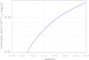 |
Fig. A.1. Mean survey luminosity limit of the CLASSIX Survey at |bII|> 20° as a function of redshift. The dashed lines show the different X-ray luminosity limits used in the study in the discussion section and the redshift limit. |
A.2. Images of the Local Supercluster members
Fig. A.1 provides images of the member groups and clusters of the Local Supercluster. The optical images are obtained from the Digital Sky Survey (DSS) scans of photographic plates3 and the contours show the X-ray surface brightness observed in the RASS.
All groups and clusters of this structure have significantly extended X-ray emission in the RASS and no peculiar X-ray spectral properties. The two groups, NGC 5813 and NGC 5846, have been observed in deep Chandra observations, NGC 5813 by Randall et al. (2015) and NGC 5846 by Machacek et al. (2011), and interesting cavities and interaction effects of the central AGN with the intragroup medium were found.
A.3. Images of the Centaurus Supercluster members
Figs. A.3 and A.4 provide images of the Centaurus SC with X-ray surface brightness contours from the RASS overlayed on optical Digital Sky Survey images. For two clusters, RXCJ1349.3-3018 (A3574E) and RXCJ1403.5-3359 (NGC5328) we also show optical images with X-ray surface brightness contours from XMM-Newton observations. For the XMM-Newton data the exposures of the three detectors were combined with a scaling of the pn-images by a factor of 3.3 with respect to the MOS images.
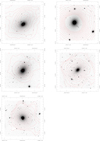 |
Fig. A.2. Images of the Local Supercluster. Shown are contours of the X-ray surface brightness superposed on optical Digital Sky Survey images. All images in this and the following sections are oriented such that north is up and east to the left. Upper left: RXCJ1226.2+1257, M86 Upper right: RXCJ1230.7+1223, M87, Middle left: RXCJ1242.8+0241, NGC 4636 Middle right: RXCJ1501.1+0141,NGC 5813 Lower left: RXCJ1506.4+0136, NGC 5846 |
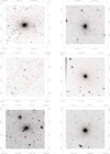 |
Fig. A.3. Members of the Centaurus Supercluster. Contours of the X-ray surface brightness superposed on optical images from the DSS database. The X-ray data are taken from the RASS or XMM-Newton observations. Upper left: RXCJ1248.7-4118, A3526, Centaurus cluster, Upper right: RXCJ1304.2-3030, NGC 4936, Middle left: RXCJ1307.2-4023, ESO-3230.0159, Middle right: RXCJ1315.3-1623, NGC 5044, Lower left: RXCJ1321.2-4342, NGC 5090/5091, Lower right: RXCJ1336.6-3357, A 3565. |
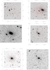 |
Fig. A.4. Members of the Centaurus Supercluster continued. Upper left: RXCJ1347.2-3025, A 3574 W Upper right: RXCJ1349.3-3018, A 3574 E Middle left: XMM-Newton image of RXCJ1349.3-3018, A3574 E Middle right: RXCJ1352.8-2829, NGC 5328, Lower left: RXCJ1403.5-3359, AS 753 Lower right: XMM-Newton image of RXCJ1403.5-3359, AS 753. |
All members of the Centaurus SC shown here have significantly extended X-ray emission in the RASS and no peculiar X-ray spectral properties. An exception is the cluster RXCJ1349.3-3018 (A3574E) which harbours an X-ray bright Sy 1.2 galaxy, IC4329A, which outshines the cluster. In the RASS image, which is shown in Fig. A.4 upper right, we see mostly a point source and the additional cluster emission is difficult to distinguish. Using, however, a pointed ROSAT observation and even better an observation with XMM-Newton (shown in Fig. A.4 middle left) we could separate the soft point source emission from the AGN to get approximate values for the cluster emission. This deblended X-ray luminosity is listed in Table 4.
The two components of A3574, RXCJ1347.2-3025 and RXCJ1349.3-3018, appear as two distinct X-ray emission regions in the RASS. One of the Centaurus SC members, RXCJ1321.2-4342, NGC 5090/5091 is located in the ZoA, at bII ∼ 18.8°.
A.4. Images of the Coma Supercluster members
In this section we provide images of the member groups and clusters of the Coma SC (Figs. A.5, A.6 and A.7). The images show overlays of X-ray contours from RASS on DSS images produced in the same way as in the previous sections. For two clusters with interesting internal structures, A1185 (RXCJ1110.5+2843) and A1367 (RXCJ1145.0+1936), we also show images with X-ray contours from XMM-Newton observations. We do not show an image of Coma because the cluster is so large and there are plenty of detailed images available in the literature, for example the new image obtained with eROSITA by Churazov et al. (2021). All groups and clusters of the Coma SC shown here have significantly extended X-ray emission in the RASS and no peculiar X-ray spectral properties.
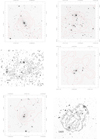 |
Fig. A.5. Members of the Coma Supercluster. Upper left: RXCJ1109.7+2146, A 1177, Upper right: RXCJ1110.5+2843, A 1185, Middle left: XMM-Newton image of RXCJ1110.5+2843, A1885. Middle right: RXCJ1122.3+2419, HCG 51, Lower left: RXCJ1145.0+1936, A1367, Lower right: XMM-Newton image of RXCJ1145.0+1936, A1367. |
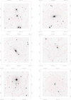 |
Fig. A.6. Members of the Coma Supercluster continued. Upper left: RXCJ1204.1+2020, NGC 4066, Upper right: RXCJ1204.4+0154, MKW4, Middle left: RXCJ1206.6+2810, NGC 410 Middle right: RXCJ1213.4+2136, UGC 7224, Lower left: RXCJ1219.8+2825,CGCG 185-075 Lower right: RXCJ1223.1+1037, NGC 4325. |
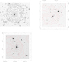 |
Fig. A.7. Members of the Coma Supercluster continued. Upper left: XMM-Newton image of RXCJ1223.1+1037, NGC 4325 Upper right: RXCJ1231.0+0037, NGC 4493, Middle left: RXCJ1334.3+3441, NGC 522. |
A.5. Images of the Hercules Supercluster members
This section provides images of the members of the Hercules supercluster at z ≤ 0.03 (Figs. A.8, A.9). The images show overlays of X-ray contours from RASS on DSS images produced in the same way as in the previous sections.
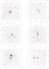 |
Fig. A.8. Members of the Hercules supercluster. Upper left: RXCJ1629.6+4049, A2197 E, Upper right: RXCJ1649.3+5325, Arp 330, Middle left: RXCJ1714.3+4341, NGC 6329, Middle right: RXCJ1715.3+5724, NGC 6338, Lower left: RXCJ1723.4+5658, NGC 6370, Lower right: RXCJ1736.3+6803, NGC 6420. |
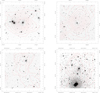 |
Fig. A.9. Members of the Hercules supercluster continued. Upper left: RXCJ1755.8+6236 in the North Ecliptic Pole region, Upper right: RXCJ1806.5+6135, VII Zw 767, Middle left: RXCJ1818.7+5017, UGC 11202 Middle right: RXCJ1941.7+5037, UGC 11465. |
Since this extension of the Hercules SC is less well known we remark on some of the cluster identifications. All groups and clusters have clearly extended X-ray emission in the RASS and no peculiar spectral properties. RXCJ1629.6+4049 is one of two parts of the cluster Abell 2197, which was found to have two clearly distinct X-ray emitting components, A2197 W and A2197 E, in the RASS (Muriel et al. 1996). The clusters RXCJ1736.3+6803 and RXCJ1755.8+6236 have already been identified in the RASS North Ecliptic Pole survey (Henry et al. 1995) and they are described in detail in this publication. RXCJ1714.3+4341 has also been found as a WBL group by White et al. (1999). RXCJ1723.4+5658 has been identified as a group of galaxies by van der Linden et al. (2007), and RXCJ1736.3+6803 by Lee et al. (2017). One of the clusters, RXCJ1941.7+5037 lies in the ZoA at bII ∼ 13.3°.
A.6. Images of the Sagittarius Supercluster members
This section provides images of the groups and clusters of the Sagittarius SC (Fig. A.10). The images show overlays of X-ray contours from RASS on DSS images produced in the same way as in the previous sections. All objects have significantly extended X-ray emission in the RASS and no unexpected spectral properties.
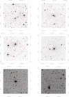 |
Fig. A.10. Members of the Sagittarius Supercluster. Upper left: RXCJ1928.2-2930, ESO 460-G004, Upper right: RXCJ1944.0-2824, NGC6816 Middle left: RXCJ2000.6-3837, Middle right: RXCJ2018.4-4102, IC 4991, Lower left: RXCJ2029.2-2240, ESO 528 - G008 Lower right: RXCJ2035.7-2513, A3698 |
A.7. Images of the Lacerta Supercluster members
This section provides images of the groups and clusters of the Lacerta SC (Fig. A.11). The images show overlays of X-ray contours from RASS on DSS images produced in the same way as in the previous sections. All objects have significantly extended X-ray emission in the RASS and no unexpected spectral properties.
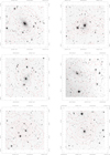 |
Fig. A.11. Members of the Lacerta Supercluster. Upper left: RXCJ2215.6+3717, NGC 7242, Upper right: RXCJ2222.4+3612, NGC 7265, Middle left: RXCJ2224.2+3608, NGC 7274, Middle right: RXCJ2231.0+3920, Lower left: RXCJ2318.6+4257, UGC 12491, Lower right: RXCJ2319.7+4251, NGC 7618. |
A.8. Properties of supplementary clusters
Table A.1 provides data on those additional clusters, which were linked to Centaurus SC and the Coma SC with the alternative linking schemes discussed in section 5.
Groups and clusters which were found with the alternative linking schemes to be SC members.
All Tables
Properties of the superclusters in the local Universe at z ≥ 0.03 constructed with a minimal linking length, l0 = 19 Mpc.
Groups and clusters which were found with the alternative linking schemes to be SC members.
All Figures
|
Fig. 1. Sky distribution of the superclusters at z ≤ 0.03 in equatorial coordinates (upper panel) and galactic coordinates (lower panel). The superclusters are marked by numbers: 1 = Perseus-Pisces Supercluster, 2 = Abell 400 supercluster, 3 = Local Supercluster, 4 = Centaurus Supercluster, 5 = Coma Supercluster 6 = Hercules supercluster, 7 = Sagittarius Supercluster, 8 = Lacerta Supercluster. The full coloured symbols are CLASSIX supercluster members, with z ≤ 0.03, while more distant members are shown by coloured open symbols. All other CLASSIX clusters at z ≤ 0.03 are shown as black open circles. The galactic band (bII = ±20°) is shown by blue dotted (dashed) lines, the region with high hydrogen column density (nH ≥ 2.5 × 1021 cm−2) is indicated by the solid blue lines, and the supergalactic band (SGZ = ±20°) by red lines. |
| In the text | |
|
Fig. 2. Supercluster multiplicity function found from observations (red). The cumulative fraction of CLASSIX clusters in superclusters as a function of the number of members is shown in blue (with corresponding axis on the right). The multiplicity function for a simulated random distribution of clusters is shown in green and the corresponding fraction of clusters in superclusters as green dashed line. |
| In the text | |
|
Fig. 3. Three-dimensional representation of the Local SC. The four objects in the lower right are the Virgo cluster, with M87, M86 and M49 as well as NGC4636. M49 is marked with an open symbol because its X-ray luminosity is below the adopted luminosity limit. |
| In the text | |
|
Fig. 4. Three-dimensional representation of the Centaurus SC (blue circles) and the Local SC (red squares). The open green squares show (from left to right) the Norma, Antlia and Hydra clusters. Other CLASSIX clusters in this volume not associated with the two SC are shown as open black circles. |
| In the text | |
|
Fig. 5. Centaurus supercluster in three projections in Supergalactic coordinates. The SC members are shown as filled blue circles, while other CLASSIX clusters in this volume are marked by open circles. The size of the symbols is proportional to the cube root of the mass of the clusters as explained in the text. Several prominent clusters are marked. 1: Centaurus cluster, A3526, 2: NGC 5044 group, 3: AS 753, 4: A 3574 West, 5: A 3574 East. |
| In the text | |
|
Fig. 6. Three-dimensional representation of the Coma SC in Supergalactic coordinates. The members of the Coma SC are shown as full blue circles, the Coma cluster is marked by a larger symbol and the two clusters at z > 0.03 are shown as open squares. All other CLASSIX clusters in the volume are shown as black open circles. |
| In the text | |
|
Fig. 7. Coma Supercluster in Supergalactic coordinates in three projections. Members of the structure are shown as filled blue circles, where the size of the symbol reflects the estimated mass of the cluster. The two clusters at z > 0.03 are shown as blue squares. All other clusters are marked by black open circles. The most massive members of the Coma supercluster are identified by numbers: 1: Coma, 2: A 1367, 3: MKW4, 4: NGC 410, 5: NGC 4325, 6: A1177, 7: A 1185. |
| In the text | |
|
Fig. 8. Three-dimensional representation of Hercules supercluster in Supergalactic coordinates. The members of the SC at z ≤ 0.03 are shown as solid blue circles, some of the structure beyond with open green circles. Other CLASSIX clusters in the study volume are marked by open black circles. |
| In the text | |
|
Fig. 9. Hercules supercluster in Supergalactic coordinates in three projections. The size of the symbols indicates their mass. Supercluster members with z ≤ 0.03 are shown as solid blue circles, those at z > 0.03 with blue squares, and other CLASSIX clusters in this volume with open black circles. The clusters with numbers are: 1 = NGC 6338, 2 = A2197W, 3 = A2199, 4 = A2197E. |
| In the text | |
|
Fig. 10. Three-dimensional representation of distribution of the members of the Sagittarius SC in Supergalactic coordinates. The galaxy groups are designated by the names of their central galaxies. |
| In the text | |
|
Fig. 11. Three-dimensional representation the Lacerta SC in Supergalactic coordinates. The galaxy groups are designated by the names of their central galaxies, except for one unmarked object, which contains the giant elliptical UC 12064 slightly off-centre. |
| In the text | |
|
Fig. 12. Three-dimensional representation of all supercluster found within z ≤ 0.03 with at least five members and a minimum linking length of l0 = 19 Mpc. The structures marked in colour are: red = Perseus-Pisces SC, red-brown = A400 SC, violet = Local SC, orange = Centaurus SC, siena = Coma SC, dark blue = Hercules SC, turquoise = Sagittarius SC, light green = Lacerta SC. Non-supercluster members are shown as black open circles. |
| In the text | |
|
Fig. 13. Cluster members of the Perseus-Pisces SC for different linking schemes. The solid black points show the SC members found for scheme 1 and the large open circles show the members found for scheme 8. The object marked by an open square is first found with scheme 5. Some prominent clusters are marked: 1 = Perseus, 2 = AWM7, 3 = A262, 4 = NGC 507, 5 = NGC 383, 6 = 3C129, 7 = UGC 12655, 8 = double cluster RXCJ2318.6+4257, RXCJ2319.7+4521, 9 = NGC7242. The blue lines constrain the region of high interstellar absorption, the red lines show galactic latitudes bII ± 20°. |
| In the text | |
|
Fig. 14. Cluster members of the Centaurus SC and the Local SC for different linking schemes. The solid circles and the red squares show the Centaurus and Virgo superclusters found with scheme 1, the crosses mark those found with scheme 2 and the large open circles mark those found with scheme 8. The open squares show two clusters linked at intermediate schemes 3 and 5, respectively. Some prominent clusters are marked: 1 = Centaurus, 2 = NGC 5044, 3 = M87, 4 = Hydra (A1060), 5 = Antlia, 6 = HCG 62, 7 = A3581, 8 = Norma (A3627), 9 = RXCJ1324.7-5736. |
| In the text | |
|
Fig. 15. Cluster members of the Coma SC for different linking schemes. The solid blue circles describe the structure found with scheme 1, while the large open squares and open circles mark the structure found with schemes 7 and 8, respectively. The green squares show the clusters linked with scheme 3. Some prominent clusters are marked: 1 = Coma cluster, 2 = A 1367, 3 = MKW4, 4 = NGC 4325, 5 = NGC 410, 6 = NGC 5171. |
| In the text | |
|
Fig. 16. Cumulative normalised X-ray luminosity distribution of clusters in the eight superclusters (red dashed line) compared to the distribution for clusters in the field (blue solid line). |
| In the text | |
|
Fig. 17. Cumulative normalised X-ray luminosity distribution of clusters in the eight superclusters (red dashed line) compared to the distribution for clusters in the field (blue solid line) with a lower X-ray luminosity limit of 0.5 × 1043 erg s−1. The data in the left panel include all eight superclusters, those in the right panel only the four large superclusters. |
| In the text | |
|
Fig. A.1. Mean survey luminosity limit of the CLASSIX Survey at |bII|> 20° as a function of redshift. The dashed lines show the different X-ray luminosity limits used in the study in the discussion section and the redshift limit. |
| In the text | |
|
Fig. A.2. Images of the Local Supercluster. Shown are contours of the X-ray surface brightness superposed on optical Digital Sky Survey images. All images in this and the following sections are oriented such that north is up and east to the left. Upper left: RXCJ1226.2+1257, M86 Upper right: RXCJ1230.7+1223, M87, Middle left: RXCJ1242.8+0241, NGC 4636 Middle right: RXCJ1501.1+0141,NGC 5813 Lower left: RXCJ1506.4+0136, NGC 5846 |
| In the text | |
|
Fig. A.3. Members of the Centaurus Supercluster. Contours of the X-ray surface brightness superposed on optical images from the DSS database. The X-ray data are taken from the RASS or XMM-Newton observations. Upper left: RXCJ1248.7-4118, A3526, Centaurus cluster, Upper right: RXCJ1304.2-3030, NGC 4936, Middle left: RXCJ1307.2-4023, ESO-3230.0159, Middle right: RXCJ1315.3-1623, NGC 5044, Lower left: RXCJ1321.2-4342, NGC 5090/5091, Lower right: RXCJ1336.6-3357, A 3565. |
| In the text | |
|
Fig. A.4. Members of the Centaurus Supercluster continued. Upper left: RXCJ1347.2-3025, A 3574 W Upper right: RXCJ1349.3-3018, A 3574 E Middle left: XMM-Newton image of RXCJ1349.3-3018, A3574 E Middle right: RXCJ1352.8-2829, NGC 5328, Lower left: RXCJ1403.5-3359, AS 753 Lower right: XMM-Newton image of RXCJ1403.5-3359, AS 753. |
| In the text | |
|
Fig. A.5. Members of the Coma Supercluster. Upper left: RXCJ1109.7+2146, A 1177, Upper right: RXCJ1110.5+2843, A 1185, Middle left: XMM-Newton image of RXCJ1110.5+2843, A1885. Middle right: RXCJ1122.3+2419, HCG 51, Lower left: RXCJ1145.0+1936, A1367, Lower right: XMM-Newton image of RXCJ1145.0+1936, A1367. |
| In the text | |
|
Fig. A.6. Members of the Coma Supercluster continued. Upper left: RXCJ1204.1+2020, NGC 4066, Upper right: RXCJ1204.4+0154, MKW4, Middle left: RXCJ1206.6+2810, NGC 410 Middle right: RXCJ1213.4+2136, UGC 7224, Lower left: RXCJ1219.8+2825,CGCG 185-075 Lower right: RXCJ1223.1+1037, NGC 4325. |
| In the text | |
|
Fig. A.7. Members of the Coma Supercluster continued. Upper left: XMM-Newton image of RXCJ1223.1+1037, NGC 4325 Upper right: RXCJ1231.0+0037, NGC 4493, Middle left: RXCJ1334.3+3441, NGC 522. |
| In the text | |
|
Fig. A.8. Members of the Hercules supercluster. Upper left: RXCJ1629.6+4049, A2197 E, Upper right: RXCJ1649.3+5325, Arp 330, Middle left: RXCJ1714.3+4341, NGC 6329, Middle right: RXCJ1715.3+5724, NGC 6338, Lower left: RXCJ1723.4+5658, NGC 6370, Lower right: RXCJ1736.3+6803, NGC 6420. |
| In the text | |
|
Fig. A.9. Members of the Hercules supercluster continued. Upper left: RXCJ1755.8+6236 in the North Ecliptic Pole region, Upper right: RXCJ1806.5+6135, VII Zw 767, Middle left: RXCJ1818.7+5017, UGC 11202 Middle right: RXCJ1941.7+5037, UGC 11465. |
| In the text | |
|
Fig. A.10. Members of the Sagittarius Supercluster. Upper left: RXCJ1928.2-2930, ESO 460-G004, Upper right: RXCJ1944.0-2824, NGC6816 Middle left: RXCJ2000.6-3837, Middle right: RXCJ2018.4-4102, IC 4991, Lower left: RXCJ2029.2-2240, ESO 528 - G008 Lower right: RXCJ2035.7-2513, A3698 |
| In the text | |
|
Fig. A.11. Members of the Lacerta Supercluster. Upper left: RXCJ2215.6+3717, NGC 7242, Upper right: RXCJ2222.4+3612, NGC 7265, Middle left: RXCJ2224.2+3608, NGC 7274, Middle right: RXCJ2231.0+3920, Lower left: RXCJ2318.6+4257, UGC 12491, Lower right: RXCJ2319.7+4251, NGC 7618. |
| In the text | |
Current usage metrics show cumulative count of Article Views (full-text article views including HTML views, PDF and ePub downloads, according to the available data) and Abstracts Views on Vision4Press platform.
Data correspond to usage on the plateform after 2015. The current usage metrics is available 48-96 hours after online publication and is updated daily on week days.
Initial download of the metrics may take a while.