| Issue |
A&A
Volume 633, January 2020
|
|
|---|---|---|
| Article Number | A19 | |
| Number of page(s) | 12 | |
| Section | Cosmology (including clusters of galaxies) | |
| DOI | https://doi.org/10.1051/0004-6361/201936400 | |
| Published online | 23 December 2019 | |
Observational evidence for a local underdensity in the Universe and its effect on the measurement of the Hubble constant⋆
1
University Observatory, Ludwig-Maximilians-Universität München, Scheinerstr. 1, 81679 München, Germany
e-mail: This email address is being protected from spambots. You need JavaScript enabled to view it.
2
Astrophysics Research Institute, Liverpool John Moores University, IC2, Liverpool Science Park, 146 Brownlow Hill, Liverpool L3 5RF, UK
Received:
29
July
2019
Accepted:
4
November
2019
Abstract
For precision cosmological studies it is important to know the local properties of the reference point from which we observe the Universe. Particularly for the determination of the Hubble constant with low-redshift distance indicators, the values observed depend on the average matter density within the distance range covered. In this study we used the spatial distribution of galaxy clusters to map the matter density distribution in the local Universe. The study is based on our CLASSIX galaxy cluster survey, which is highly complete and well characterised, where galaxy clusters are detected by their X-ray emission. In total, 1653 galaxy clusters outside the “zone of avoidance” fulfil the selection criteria and are involved in this study. We find a local underdensity in the cluster distribution of about 30–60% which extends about 85 Mpc to the north and ∼170 Mpc to the south. We study the density distribution as a function of redshift in detail in several regions in the sky. For three regions for which the galaxy density distribution has previously been studied, we find good agreement between the density distribution of clusters and galaxies. Correcting for the bias in the cluster distribution we infer an underdensity in the matter distribution of about −30 ± 15% (−20 ± 10%) in a region with a radius of about 100 (∼140) Mpc. Calculating the probability of finding such an underdensity through structure formation theory in a ΛCDM universe with concordance cosmological parameters, we find a probability characterised by σ-values of 1.3 − 3.7. This indicates low probabilities, but with values of around 10% at the lower uncertainty limit, the existence of an underdensity cannot be ruled out. Inside this underdensity, the observed Hubble parameter will be larger by about 5.5 +2.1−2.8%, which explains part of the discrepancy between the locally measured value of H0 compared to the value of the Hubble parameter inferred from the Planck observations of cosmic microwave background anisotropies. If distance indicators outside the local underdensity are included, as in many modern analyses, this effect is diluted.
Key words: galaxies: clusters: general / cosmology: observations / large-scale structure of Universe / distance scale / X-rays: galaxies: clusters
Based on observations at the European Southern Observatory La Silla, Chile and the German-Spanish Observatory at Calar Alto.
© H. Böhringer et al. 2019
 Open Access article, published by EDP Sciences, under the terms of the Creative Commons Attribution License (http://creativecommons.org/licenses/by/4.0), which permits unrestricted use, distribution, and reproduction in any medium, provided the original work is properly cited.
1. Introduction
As an integral part of the cosmic large-scale structure, galaxy clusters are reliable tracers of the underlying dark matter distribution. Since they form the largest peaks in the initially random Gaussian density fluctuation field, their density distribution can be statistically closely related to the matter density distribution (e.g. Bardeen et al. 1986). Cosmic structure formation theory has shown that the ratio of the cluster density fluctuation amplitude is biased with respect to the matter density fluctuations in the sense that the cluster density fluctuations have a larger variance. The ratio of the rms amplitude of the cluster density to that of the dark matter, which is referred to as bias, is practically independent of scale (e.g. Kaiser 1986; Mo & White 1996; Sheth & Tormen 1999; Tinker et al. 2010).
We have already found good observational support for this concept with our galaxy cluster surveys (Böhringer & Huchra 2000; Böhringer et al. 2004, 2013, 2017a). We showed that the density fluctuation power spectrum of galaxy clusters is an amplified version of the power spectrum of galaxies and of the inferred power spectrum of the underlying dark matter distribution, where the bias is dependent on the lower cluster mass limit exactly as predicted from theory (Balaguera-Antolinez et al. 2010, 2011). We further demonstrated with simulations that the cluster density in local overdensities follows the matter distribution. This was shown with superstes-clusters, superclusters that were constructed such that they would collapse in the future (Chon et al. 2015).
In this paper we exploit this property of galaxy clusters to study the matter density distribution in the local Universe. For the study we used our CLASSIX (Cosmic Large-Scale Structure in X-rays) galaxy cluster survey, the combination of the REFLEX and NORAS surveys (Böhringer & Huchra 2000; Böhringer et al. 2004, 2013, 2017a), plus an extension into the “zone of avoidance”. This data set constitutes the most complete and well characterised galaxy cluster sample in the nearby Universe allowing a sufficiently dense sampling of the clusters to map the cluster density distribution.
There has been increasing interest in understanding the density distribution in the local Universe, because the properties of the local reference point from which we observe the Universe are important for conducting cosmological precision measurements. This is most apparent for measurements of the Hubble constant performed with local distance standards. Historically, when evidence for an accelerating universe came from observations of distant type Ia supernovae (SNIa; Perlmutter et al. 1999; Schmidt et al. 1998), models with local voids were considered as an alternative explanation of the SN data without dark energy or a cosmological constant (e.g. Célérier 2000; Tomita 2000, 2001; Alexander et al. 2009; February et al. 2010 and references therein). A minimum void model would require a void size of at least about  Mpc with a mean mass density deficiency of ∼40% to explain the SN data in a universe without a cosmological constant (e.g. Alexander et al. 2009). Today, with more precise SN data filling the redshift range very densely, this void model mimicking an accelerated universe can be ruled out (e.g. Kenworthy et al. 2019). Such void models have also been critically discussed by Moss et al. (2011) and Marra et al. (2013). In addition, our previous study on the cluster distribution in the REFLEX II survey ruled out such a large spherical local void (Böhringer et al. 2015).
The debate over the discrepancy between the Hubble constant measured locally of about 74.0 (±1.4) km s−1 Mpc−1 (e.g. Riess et al. 2018a,b, 2019) and the value inferred from the Planck survey of 67.4 (±0.5) km s−1 Mpc−1 (Planck Collaboration XIII 2016; Planck Collaboration VI 2019) has kept alive the discussion about a local underdensity (e.g. Riess et al. 2018b, 2019; Shanks et al. 2019a,b). If our local cosmic neighbourhood has less than the mean cosmic density, then the Hubble constant observed locally is larger than that measured on large scale.
Different tracers have been used to study the local density distribution. Using SNIa, Zehavi et al. (1998) and Jha et al. (2007) claimed the detection of a local underdensity, while Hudson et al. (2004) and Conley et al. (2007) do not find such evidence. Giovanelli et al. (1999) characterised the local Hubble flow out to 200 h−1 Mpc with galaxy clusters and find hardly any variations. Huang et al. (1997), Frith et al. (2003, 2006), Busswell et al. (2004), and Keenan et al. (2013) found a local underdensity in the galaxy distribution. In a more recent study Whitbourn & Shanks (2014) traced the galaxy distribution in three larger regions, in the South Galactic Cap (SGC), the southern part of the North Galactic Cap (NGC), and the northern part of the NGC using 2MASS K-band magnitudes in connection with 6dFRGS, GAMA, and SDSS spectroscopic data out to z = 0.1. They find a large underdense region with a deficit of about 40% inside a radius of 150 h−1 Mpc in the SGC, no deficit in the southern part of the NGC, and a less pronounced underdensity in the NGC north of the equator.
While most of these studies cover only a limited region of the sky, CLASSIX allows us to study the local density distribution over most of the sky area. In our previous study based on the REFLEX II survey we found evidence for a southern underdensity out to about 170 Mpc (Böhringer et al. 2015). Here we studied the entire extragalactic sky to investigate the local density distribution. We also explore the diagnostics and systematic errors in more detail.
The paper is organised as follows. In Sect. 2 we give a brief description of the survey and its characteristics and explain our method in Sect. 3. In Sect. 4.1 we explore the local underdensity monopole, show results for different hemispheres in Sect. 4.2, and for particular regions in Sect. 4.4. In Sect. 4.3 we study cumulative density distributions of clusters and derive the distribution of matter. We discuss the results in Sects. 5 and 6 provides a summary and conclusion. Several technical points are explained in the appendix. For the determination of all parameters that depend on distance we use a flat ΛCDM cosmology with the parameters H0 = 70 km s−1 Mpc−1 and Ωm = 0.3. Exceptions are results quoted from the literature, for which the scaling is given explicitly.
2. The CLASSIX galaxy cluster survey
This study requires a cluster sample that traces the local Universe sufficiently densely, is statistically highly complete, and has a well-known selection function. The best data base is at this moment our CLASSIX galaxy cluster catalogue (Böhringer et al. 2016). It is the combination of our surveys in the southern sky, REFLEX II (Böhringer et al. 2013), and the northern hemisphere, NORAS II (Böhringer et al. 2017a). Together they cover 8.26 ster of the sky at Galactic latitudes |bII| ≥ 20° and the cluster catalogue contains 1773 members (of which 1653 are used here). In this study we did not excise the regions of the Magellanic Clouds or the VIRGO cluster (except when explicitly noted). In the completed survey we find no significant deficit in the cluster density in these sky areas. We also use an extension of CLASSIX to lower Galactic latitudes into the zone of avoidance. This region is restricted to the area with an interstellar hydrogen column density nH ≤ 2.5 × 1021 cm−2, because in regions with higher column density, X-rays are strongly absorbed and the sky usually has a high stellar density, making the detection of clusters in the optical extremely difficult. The values for the interstellar hydrogen column density are taken from the 21 cm survey of Dickey & Lockman (1990)1. This area amounts to another 2.56 ster and altogether the survey data cover 86.2% of the sky. The spectroscopic follow-up to obtain redshifts for this part of the survey is only about 70% complete and furthermore the completeness of the cluster sample is not as high as for REFLEX and NORAS. The cluster density we show for the zone of avoidance is therefore a lower limit.
The CLASSIX galaxy cluster survey and its extension is based on the X-ray detection of galaxy clusters in the ROSAT All-Sky Survey (RASS, Trümper 1993; Voges et al. 1999). The source detection for the survey, the construction of the survey, and the survey selection function as well as tests of the completeness of the survey are described in Böhringer et al. (2013, 2017a). In summary, the nominal unabsorbed flux limit for the galaxy cluster detection in the RASS is 1.8 × 10⁻¹² erg s−1 cm−2 in the 0.1–2.4 keV energy band. For the assessment of the large-scale structure in this paper we apply an additional cut on the minimum number of detected source photons of 20 counts. This has the effect that the nominal flux limit quoted above is only reached in about 80% of the survey. In regions with lower exposure and higher interstellar absorption, the flux limit is accordingly higher (see Fig. 11 in Böhringer et al. 2013 and Fig. 5 in Böhringer et al. 2017a). This effect is modelled and taken into account in the survey selection function.
We have already demonstrated with the REFLEX I survey (Böhringer et al. 2004) that clusters provide a precise means to obtain a census of the cosmic large-scale matter distribution through for example the correlation function (Collins et al. 2000), the power spectrum (Schuecker et al. 2001, 2002, 2003a; Schuecker et al. 2003b), Minkowski functionals, (Kerscher et al. 2001), and, using REFLEX II, with the study of superclusters (Chon & Böhringer 2013; Chon et al. 2014) and the cluster power spectrum (Balaguera-Antolinez et al. 2011, 2012). The fact that clusters follow the large-scale matter distribution in a biased way as mentioned above, is a valuable advantage, which makes it easier to detect local density variations.
Relevant physical parameters for clusters were determined in the following way. X-ray luminosities in the 0.1–2.4 keV energy band have been derived within a cluster radius of r5002. To estimate the cluster mass and temperature from the observed X-ray luminosity we use the scaling relations described in Pratt et al. (2009). These were determined from a representative cluster sub-sample of our survey, called REXCESS (Böhringer et al. 2007). Since the radius r500 is determined from the cluster mass, the calculation of X-ray luminosity inside r500, cluster mass, and temperature were performed iteratively, as described in Böhringer et al. (2013). The definitive identification of the clusters and the redshift measurements are described in Guzzo et al. (2009), Chon & Böhringer (2012), and Böhringer et al. (2013).
The survey selection function was determined as a function of the sky position with an angular resolution of one degree and as a function of redshift. The selection function takes all the systematics of the RASS exposure distribution, Galactic absorption, the fiducial flux, and the detection count limit into account. The interstellar hydrogen column density for these calculations is taken from Dickey & Lockman (1990). The selection function as a function of sky position and redshift was published for REFLEX II in the online material of Böhringer et al. (2013) and for NORAS II in Böhringer et al. (2017a).
3. Methods
We studied the density distribution of clusters and of the underlying matter distribution as a function of redshift in different regions of the sky. Because we used a flux-limited cluster sample with additional smaller sensitivity variations in regions of the sky with shorter exposures, we could not use the cluster number distribution directly without taking the selection function into account. In the following we used two different methods to achieve this.
In the first method we compared the observed cluster counts in redshift bins with the expected counts. The expected counts were calculated from the observed X-ray luminosity function convolved with the survey selection function, which is given as a function of redshift and sky position. For the luminosity function we took the best-fitting Schechter function for the REFLEX II cluster survey from Böhringer et al. (2014). The X-ray luminosity function for NORAS II is the same within the uncertainty limits (Böhringer et al. 2017a,b). The REFLEX II luminosity function is shown in Fig. A.1 and the parameters for the Schechter function are listed in Table A.1, where we also give the parameters for the bracketing lower and upper limit functions. We did not detect any significant evolution in the X-ray luminosity function in the redshift range z = 0 − 0.4, as shown and explained in detail in Böhringer et al. (2014). We therefore assume this function to be constant over the distance range considered here. The relative density variations were then determined by the ratio of the observed to the expected number of galaxy clusters.
The second method was used to derive the unbinned cumulative mean density of clusters as a function of redshift. In this approach we attributed weights to each cluster to correct for the spatially varying survey limits. The weights were calculated from an integration of the luminosity function, ϕ(LX), as follows:
 (1)
(1)
where LX0 is the nominal lower limit of the sample and LXi is the lower X-ray luminosity limit at the sky location and redshift of the cluster. We then determined the relative density distribution of the clusters by comparing the observed distribution of the clusters with weights to the prediction of the cluster density for a volume complete sample with a limiting luminosity of LX0. We used the same technique with weights to produce maps of the projected density distribution of the clusters in redshift slices.
To infer the underlying matter distribution from the observed distribution of clusters, which is done in Sect. 4.3, we assume that the cluster distribution is biased with respect to that of the matter using the formalism of Tinker et al. (2010). We verify this approach in Appendix B with studies of cluster counts in cells in cosmological numerical simulations. We find that the uncertainty in the prediction of the matter density is roughly given by the Poisson error in the cluster number counts.
To calculate the bias factor, which is independent of scale, we used the formulas derived by Tinker et al. (2010) from large N-body simulations. We calculated the bias as a function of cluster mass for the adopted cosmological model3. For easier application, we fitted the result with a parameterised function of the following form:
 (2)
(2)
with A = 0.664, B = 0.1614, C = −1.23 × 10⁻⁵, D = 1.152, and E = 0.320, where m is the cluster mass, M200, in units of  .
.
The cluster mass was determined from the observed X-ray luminosity by means of the X-ray luminosity–mass relation described in Böhringer et al. (2014), the same scaling relation used to determine r500 above. The mass estimate for individual clusters has an estimated uncertainty of about 40% (e.g. Pratt et al. 2009). This translates into an uncertainty in the bias factor of not more than 5%, which we take into account in our modelling.
4. Results
4.1. CLASSIX survey
In Fig. 1 we show the relative density distribution of the clusters for the entire CLASSIX cluster sample with LX ≥ 1042 erg s−1 out to a redshift of z = 0.3, excluding the zone of avoidance. This distribution was constructed by dividing the observed number of CLASSIX clusters in different redshift bins by the prediction based on the best-fitting Schechter X-ray luminosity function and the CLASSIX selection function. All the relative differential density distributions of clusters shown in the following are constructed in this fashion. Here, 211 clusters are involved in tracing the density at z ≤ 0.04 and 1570 out to z = 0.3. While the overall cluster distribution is remarkably homogeneous, we note an underdensity of about 30–50% at z ≤ 0.03 (∼120 Mpc).
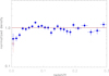 |
Fig. 1. Cluster density distribution as a function of redshift for the CLASSIX galaxy clusters covering the sky at |bII| ≥ 20° for a minimum luminosity of 1042 erg s−1 (0.1–2.4 keV). The density distribution has been normalised by the expected cluster density based on the average luminosity function as explained in Sect. 3. The open square shows the result if the region of the Virgo cluster is excluded from the analysis. |
Because we are part of the Local Supercluster with the Virgo cluster at its centre (where M 87, M 86, and M 49 enter our catalogue as separate mass halos) and since the X-ray emission of Virgo is partly blinding the region behind the cluster, one could question if the sky region of the Virgo cluster should be included in our study. The open square in Fig. 1 demonstrates that exclusion of the Virgo region has no effect on the further results of this paper.
Care needs to be taken in the interpretation of the local underdensity observed in Fig. 1. Since the region at very low redshifts, which appears underdense, is traced mostly by objects with low X-ray luminosity, which are only detected in this region, there is some degeneracy in the determination of the X-ray luminosity function at the low-luminosity end and the relative cluster density distribution in the nearby Universe. An overestimate of the X-ray luminosity function at the low-luminosity end would produce an artificial underdensity with the method applied here.
A way to break this ambiguity is to study a volume-limited sample of clusters with a homogeneous lower X-ray luminosity limit over a region that is larger than the observed underdensity. In Fig. 2 we show the mean lower luminosity limit of the CLASSIX survey as a function of redshift4. We note that for example for an X-ray luminosity limit of 2 × 1043 erg s−1 we can sample the cluster density in a volume-limited way out to a redshift of z = 0.062, larger than the underdense region. Therefore we constructed several cluster samples with a range of lower limiting luminosities (LX0 = 0.02, 0.05, 0.1, 0.2 × 1044 erg s−1), which are volume limited out to z = 0.021, 0.032, 0.044, 0.062, respectively. The density distributions of these samples are shown in Fig. 3. There is good agreement between the different samples and they all trace a similar local underdensity. Therefore the observed deficit cannot simply be the result of an inaccurately determined X-ray luminosity function. We had shown a similar exercise with the REFLEX II survey in Böhringer et al. (2015) with the same conclusion.
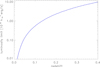 |
Fig. 2. Mean X-ray luminosity limit as a function of redshift for the CLASSIX survey. |
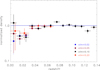 |
Fig. 3. CLASSIX galaxy cluster density distribution as a function of redshift for four different lower X-ray luminosity limits, given in the plot by the parameter xlim in units of 1044 erg s−1. All samples trace the same local density deficit. |
4.2. Different hemispheres
Figure 4 shows the projected density distribution of the clusters in the redshift range z = 0 − 0.04. The colour-coded density distribution is that of the clusters with weights smoothed by a Gaussian filter with a σ-value of 10°. The density has been normalised by the mean, so that the light(dark) regions show overdensities (underdensities). We clearly note that the distribution is not homogeneous, and so we do not expect to observe the same density deficit as noted in the mean radial profile in Fig. 1 in all sky directions. In the following we therefore study how the local density distribution depends on the region in the sky.
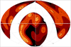 |
Fig. 4. Sky distribution of the clusters (black dots) and their surface density in the CLASSIX survey at |bII| ≥ 20° smoothed with a Gaussian filter with σ = 10° in the redshift slice z = 0 − 0.04 in equatorial coordinates. The colour coding for the density normalised to the mean is orange: > 2, red: 1 − 2, brown: 0.5 − 1, and dark brown/black: < 0.5. |
In Fig. 5 we show the cluster density distribution in the northern sky (NORAS II) and southern sky (REFLEX II) at |bII| ≥ 20°. Here the REFLEX II survey extends towards the north to a declination of +2.5°, overlapping slightly with the NORAS II survey. While the extent of the local deficit in the north reaches a redshift of about z ∼ 0.02 (∼85 Mpc), that in the southern sky stretches out to about z ∼ 0.04 (∼170 Mpc). At larger reshifts the distribution is again relatively homogeneous.
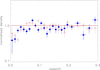 |
Fig. 5. Cluster density distribution as a function of redshift for the REFLEX II survey in the southern sky (open red circles) and the NORAS II survey in the north (filled blue circles) at |bII| ≥ 20°, for a minimum luminosity of 1042 erg s−1 (0.1–2.4 keV). The density distribution has been normalised by the expected cluster density based on the average luminosity function as explained in Sect. 3. |
The density distributions in the northern and southern Galactic hemisphere (at |bII| ≥ 20°) are compared in Fig. 6. The underdensity is less pronounced in the northern Galactic cap, with a deficit of about 35% at z ≤ 0.03 compared to about 47% in the south. In the south the density deficit stretches out to about 130 Mpc.
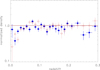 |
Fig. 6. Cluster density distribution as a function of redshift in the northern Galactic cap (filled blue circles) and southern Galactic cap (open red circles) at |bII| ≥ 20°, for a minimum luminosity of 1042 erg s−1 (0.1–2.4 keV). The density distribution has been normalised by the expected cluster density based on the average luminosity function as explained in Sect. 3. |
To see if the local cluster density in the sky outside the band of the Galaxy may be compensated by an overdensity in the zone of avoidance, we looked into our incomplete survey of this region. Figure 7 shows the cluster distribution across the sky, now with part of the region of the zone of avoidance, which is covered by our survey. The survey area is limited by an interstellar hydrogen column density of nH ≤ 2.5 × 1021 cm−2. We also show the region with a limit of nH ≤ 1.5 × 1021 cm−2 bounded by white contours that was explored alternatively. The figure shows in addition the Galactic band (|bII| ≥ 20°, black lines) and the location of the Supergalctic plane.
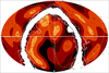 |
Fig. 7. Sky distribution of the clusters and their surface density in the CLASSIX survey with the extension into the zone of avoidance in equatorial coordinates. The survey is bounded by an interstellar hydrogen column density limit of nH ≤ 2.5 × 1021 cm−2. The white contours show the hydrogen column density boundary of nH = 1.5 × 1021 cm−2. The red lines indicate the Galactic latitudes of |bII|= ± 20°. The yellow dashed line marks the Supergalactic plane and the colour coding is the same as in Fig. 4. |
The zone of avoidance does not show any large local overdense regions as displayed in Fig. 8. We roughly expect that our survey has a completeness of about 60–70% including the incomplete spectroscopy follow-up. This incompleteness is at least partly responsible for the lower value of the mean density in the figure. We note that so far we have no evidence of an overdensity of clusters behind the band of the Galaxy.
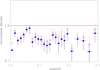 |
Fig. 8. Cluster density distribution as a function of redshift in the zone of avoidance at |bII|< 20°. Filled symbols are for the region with a Galactic hydrogen column density of nH < 2.5 × 1021 cm−2 and open symbols for nH < 1.5 × 1021 cm−2. The cluster sample in these region is not complete and therefore the data provide a lower limit. The density distribution has been normalised by the expected cluster density based on the average luminosity function as explained in Sect. 3. |
4.3. Cumulative densities
To probe the density distribution on a finer scale we now use the second method described in Sect. 3 to show the unbinned cumulative density of the clusters, that is the mean density inside a certain distance taken at the redshift of each cluster. For this we sum the clusters multiplied with their weights and compare this with the number of clusters we would expect in a volume-limited sample out to the same distance with the adopted lower luminosity limit of the analysis.
In Fig. 9 we show the cumulative density distribution of the REFLEX II clusters in the southern sky normalised to the mean density. To minimise the influence of the low-luminosity end of the X-ray luminosity function we used a lower luminosity limit of LX0 = 5 × 1042 erg s−1 here. The plot shows that the underdensity reaches out to about z ∼ 0.04 as in the differential plot above, but despite the local overdensity at the boundary of the underdense region, the cumulative mean density is only recovered at z ∼ 0.06. We also show the uncertainty limits as a red region, which takes into account the uncertainty of the X-ray luminosity function (Fig. A.1) used for the normalisation and the Poisson error of the cluster number counts.
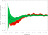 |
Fig. 9. Cumulative density distribution of REFLEX II clusters as a function of redshift normalised to the mean for a lower X-ray luminosity limit of LX0 = 5 × 1042 erg s−1 (lower curve with red uncertainty limits). The upper curve with green uncertainty limits shows the inferred dark matter distribution after correcting for the cluster bias. |
Figure 9 also shows the inferred underlying matter distribution traced by the clusters. We derive this by accounting for the fact that clusters follow the matter distribution in a biased way. We corrected for the bias in the way described in Sect. 3 and included an additional uncertainty in the estimated bias factor due to uncertainties in the mass of galaxy clusters. We note a mean matter underdensity of about −27 ± 15% out to z ∼ 0.033 (∼140 Mpc) and of about −20 ± 10% out to z ∼ 0.045 (∼190 Mpc).
Figure 10 shows in a similar way the cumulative cluster density distribution in the northern sky at |bII| ≥ 20°. The local underdensity is deeper (−50%±20%), but at this depth it only extends to about 90 Mpc. In the cumulative density we see, after a sharp density increase, a slow recovery of the mean density which is reached at z ∼ 0.07. For a mean matter underdensity of −30%±15% the extent of the region is about 100 Mpc (z ∼ 0.024) and for −20%±10% it reaches 130 Mpc (z ∼ 0.03).
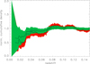 |
Fig. 10. Cumulative density distribution of NORAS II clusters as a function of redshift normalised to the mean for a lower X-ray luminosity limit of LX0 = 5 × 1042 erg s−1 (lower curve with red uncertainty limits). The upper curve with green uncertainty limits shows the inferred dark matter distribution after correcting for the cluster bias. |
In Fig. 11 we show the same plot for the entire CLASSIX survey at |bII| ≥ 20°. The results show approximately a mean behaviour of that of the two hemispheres. For a mean matter underdensity of −30%±15% the extent of the region is about 100 Mpc (z ∼ 0.0235) and for −20%±10% it reaches about 140 Mpc (z ∼ 0.033).
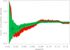 |
Fig. 11. Cumulative density distribution of CLASSIX clusters as a function of redshift normalised to the mean for a lower X-ray luminosity limit of LX0 = 5 × 1042 erg s−1 (lower curve with red uncertainty limits). The upper curve with green uncertainty limits shows the inferred dark matter distribution after correcting for the cluster bias. |
4.4. Particular sky regions
We also inspected the density distribution in smaller regions of the sky. However, the smaller number statistics increases the uncertainties. We have already analysed two particular regions in our earlier study of the southern sky, where we can compare our cluster distribution to observations of the galaxy density distribution from Whitbourn & Shanks (2014). These are the sky areas labelled A and B in Fig. 12. We found remarkably good agreement between galaxy density and cluster density in these sky areas (Böhringer et al. 2015, Figs. 8 and 9).
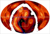 |
Fig. 12. Sky distribution of the clusters and their surface density in the extended CLASSIX survey in equatorial coordinates. Particular regions marked and labelled in the figure are explained in the text. The red lines mark the Galactic latitudes |bII| ± 20° and the displayed survey region is limited by an interstellar hydrogen column density value of nH ≤ 2.5 × 1021 cm−2. The yellow lines mark the boundaries of regions A to C and the blue lines those of regions D to F. |
The third region studied by Whitbourn & Shanks (2014) in the equatorial northern part of the north Galactic cap, region C in Fig. 12, is explored in Fig. 13. There is no underdense region in this area, except for the redshift bin z = 0.01 − 0.02 where we find no cluster above our flux limit. The galaxy distribution follows that of the clusters closely and in the redshift bin where we detect no cluster, we also note a pronounced underdensity in the distribution of galaxies. The fact that galaxies and clusters show approximately the same density distribution provides further strong support that the CLASSIX clusters are fair tracers of the underlying matter distribution.
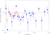 |
Fig. 13. Density distribution of CLASSIX clusters as a function of redshift in the region labelled C in Fig. 12. We find no cluster in the second redshift bin marked by a downward pointing triangle. The galaxy distribution (Whitbourn & Shanks 2014) in the same area is shown by smaller red points with error bars. There is good agreement between both density distributions. |
To further explore the variance in the cluster density distribution in different celestial regions, we selected a few sky areas that show a particularly high or low density in Fig. 12. The regions labelled D and E in the figure (with right ascension and declination ranges of RA = 55 − 115°, Dec ≤ 0° and RA ≤ 45 ° , ≥ 270°, Dec ≤ 0°, respectively and |bII| ≥ 20°) are shown in the top panel of Fig. 14. While the denser region D shows a nearby cluster deficit, the region is characterised by an overdensity at redshift z = 0.03 − 0.04. The region E around the south Galactic pole shows a particularly pronounced underdensity. In the northern sky we have the region F (RA ≤ 50 ° , ≥ 330°, Dec ≥ 0° and |bII| ≥ 20°) which shows a higher-than-average density in Fig. 12. The density distribution of F shown in the bottom panel of Fig. 14 is mostly overdense and does not contribute to the overall local underdensity at all. In summary we note that the underdensity in the local Universe has a complex structure and a homogeneous spherical void would be a rather crude representation of its geometry.
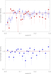 |
Fig. 14. Top: density distribution of CLASSIX clusters as a function of redshift in the high-density region in the southern sky, D (red filled circles), and the low-density region, E (blue open circles). Bottom: density distribution of CLASSIX clusters as a function of redshift in the northern high-density region, F. This seems to be one of the densest regions at z ≤ 0.04. |
5. Discussion
Combining the results from Sect. 4.3, we infer from the observed cumulative cluster density distribution a local underdensity with a deficit of −0.3 ± 0.15 extending about 100 Mpc to the north and of −0.27 ± 0.15 extending about 140 Mpc to the south. This underdensity is bounded by well-known superclusters. In the northern sky it ends at the Great Wall, while in the south its boundary is at the Shapley supercluster and two further superclusters, RXSC J0338−5414 (at z = 0.0603) and RXSC J0624−5319 (at z = 0.0520), identified by Chon & Böhringer (2013) in our survey. These superstructures seem to terminate the underdensity. Among the superclusters in the local Universe, the Shapley supercluster is by far the most prominent structure (e.g. Sheth & Diaferio 2011; Chon et al. 2015). Therefore, one way to put the observation of the local underdensity into perspective is to note that we do not live near one of the prominent superstructures. The Local Supercluster (e.g. de Vaucouleurs 1959) is not one of the massive superclusters. Therefore, the large-scale mean matter density of the Universe seems to be fairly sampled only when the volume is large enough to include also the very massive superstructures.
An important question to ask is how likely it is to find the observed extended underdensity in a Universe described by the concordance ΛCDM cosmological model. To answer the question we adopted an approximate description of the observed underdensity by a spherical region with a radius of about 100 Mpc radius, as found for the CLASSIX survey corresponding to an underdensity of −0.3 ± 0.15. In linear theory we can calculate the probability of finding such a region from the variance of the matter density distribution filtered by a top-hat filter with the given radius. To infer the linear density from the observed underdensity we have to correct for the extra expansion of the region in the non-linear evolution, yielding a Lagrangian radius of 92 ± 4 Mpc. Using the power spectrum for the ΛCDM cosmological model that best fits our cluster data (Böhringer et al. 2014), we can calculate the rms fluctuation amplitude for this scale. We applied CAMB (Lewis et al. 2000)5 to obtain the matter power spectrum. For the rms amplitude we obtained values of σ = 0.115 ± 0.005. Therefore, an underdensity of the above given amplitude corresponds to a 1.3 − 3.8σ deviation from the mean density. For the lower limiting value the probability of finding such an underdensity is therefore about 10%, a possibility that cannot easily be ruled out. If we look alternatively at the region which has a mean underdensity of −0.2 ± 0.1 and a radial extent of about 140 Mpc, we obtain the following values: the radius in linear approximation is ∼132 ± 4 Mpc and the rms fluctuation amplitude is σ = 0.075 ± 0.003, corresponding to a 1.4 − 3.9σ excursion. Considering these results, it seems more likely that the true values for the matter density deficit are close to our lower uncertainty limits.
Several works studied the probability of a local matter underdensity with similar results (e.g. Yu 2013; Wojtak et al. 2014; Odderskov et al. 2017; Wu & Huterer 2017; Fleury et al. 2017). Among these studies, it is interesting to mention the result of Wojtak et al. (2014), who discussed conditional probabilities. In the case where one wishes to know the probability of the density distribution observed from a random point in space, the probability of finding oneself in a void is slightly higher, since underdense regions occupy more space in non-comoving units than overdense regions. However, if one applies the condition that the observer is located in a dark matter halo with a mass of about 1013 M⊙, which may describe the properties of the Local Galaxy Group, the chance of being located in an overdense region is slightly higher. Despite the fact that the second case should be a better representation of the real situation, we seem to find ourselves in an underdense area.
Another consideration is the chance that the sky region hidden behind the Milky Way could compensate the deficit seen in the CLASSIX survey. If we take the entire region at |bII|< 20°, which is roughly half the area of CLASSIX, we would need a matter overdensity of about 60% out to a radius of 100 Mpc. Calculating the probability for this to happen in a ΛCDM cosmological model in a similar way as above, we find a σ-value for the probability of 3.8σ, hence much less likely than the value for a 30% underdensity in the CLASSIX area (2.6σ). According to Tully et al. (2019) the “Local Void”, one of the largest underdense structures nearby, is mostly hidden by the zone of avoidance. Since the analysis by Tully et al. is based on peculiar velocities, their method is also sensitive to structures not directly observed. Thus they can in principle obtain a more complete picture (in a smaller redshift region) than what we can presently map with the cluster distribution. Therefore, the existence of the Local Void in the hidden region behind the band of the Milky Way makes it even more unlikely that the zone of avoidance can compensate the observed local matter deficit.
In a recent study, Jasche & Lavaux (2019) used the 2M++ galaxy sample compiled by Lavaux & Hudson (2011) based on the 2MASS Galaxy Redshift Survey (Huchra et al. 2012) for a reconstruction of the matter density distribution in the local Universe with a Bayesian modelling technique including the use of N-body simulations for cosmic structure evolution. One of their results provides radial matter density distributions averaged in shells around our location presented in their Fig. 10. The density profile for the whole sky, shown in the left panel of that figure, features more underdense than overdense regions out to a radius of about 150 h−1 Mpc. If this differential density profile is integrated, the cumulative profile shows a mean underdensity of about 10–20% inside a radius of about 85 Mpc. The result is qualitatively very similar to ours, but the extent and the amplitude of the underdensity are somewhat smaller. With our large uncertainties the two results could be considered marginally consistent. There are however two possible reasons for the difference. First, the Bayesian method includes the ΛCDM model with approximately Planck mission constraints for the cosmological parameters as a prior, which means that the consistency with this model is also driving the results. Second, the galaxy sample is limited to redshifts below z = 0.06–0.08 (their Fig. 2). Their reference of the large-scale mean density therefore comes from a smaller volume than ours, and so it may be difficult to detect an underdensity with a larger extent than what they find. In light of these considerations we interpret both results as consistent. Figure 10 of Jasche & Lavaux (2019) also shows the radial profiles for two survey regions of Whitbourn & Shanks (2014) labelled A and B above. In both regions we observe a similar density structure as outlined by the clusters and galaxies.
If the density of the local Universe is less than the mean density, the Hubble constant measured within this volume is larger than that found at larger scales. In Appendix C we calculate how the Hubble constant depends on the density. For a deficit of −0.3 ± 0.15 we find a value for H0 which is higher by  , and for −0.2 ± 0.1 the increase of H0 would be
  . We note that these values of the Hubble constant refer to the volume of the underdensity. Most local measurements of H0 cover a larger volume, for example those of Riess et al. (2019), where the described effects are diluted in the average result. The quoted changes of H0 apply, however, to measurements inside the underdensity, like all studies based on peculiar motions; for example those of Tully et al. (2016, 2019), which imply a value of H0 of about 75 km s−1 Mpc−1.
Determining the Hubble constant in the redshift range z = 0.018 − 0.85 using a distance calibration from the analysis of Baryonic acoustic oscillations (BAOs) in the Dark Energy Survey, independent of local distance calibrators, Macaulay et al. (2019) find a Hubble constant of H0 = 67.8 ± 1.3 km s−1 Mpc−1. The good agreement with the results from the Planck mission is not surprising, since both analyses rely on the sound horizon as a calibration standard.
In a recent update on their work, Shanks et al. (2019b) modelled their data on the galaxy density distribution with a self-consistent outflow model, finding that the Hubble constant would be increased by about 2–4% inside a region with a radius of about 150 h−1 Mpc. Lukovic et al. (2019) explore the evidence of a local void with SN data from the joint light curve analysis (JLA; Betoule et al. 2014) and Pantheon sample (Scolnic et al. 2018) using a Lemaître-Tolman-Bondi cosmological model. Lukovic et al. find constraints on a local underdensity with a size of  and a density contrast of
  for JLA as well as
  and
and  for the Pantheon sample. The results are therefore consistent with homogeneity, but also within 1σ errors with a local underdensity as found by Whitbourn & Shanks (2014) and with our findings. These latter authors also study the implications for the galaxy distribution of Keenan et al. (2013), for which they obtain the constraints of a void size of
  with an underdensity of
  . This result is inconsistent with the SN data however, excluding one critical data point out of ten relaxes this discrepancy and also makes these findings more similar to our results. More stringent constraints were obtained by Kenworthy et al. (2019) with the Pantheon sample combined with the Foundation survey and the Carnegie Supernova Project, excluding a local underdensity of ∼100 Mpc in size with a density contrast of δρ/ρ > 27% at 5σ, which does not rule out our results closer to their lower limits. In summary, the SN data are not in conflict with our findings.
6. Summary and conclusion
We find a significant local underdensity at redshifts z ≤ 0.03 − 0.04 in the distribution of galaxy clusters, compared to the mean cluster density over a large volume observed out to z = 0.3 (excluding the zone of avoidance, with |bII| ≤ 20°). It is well known that clusters trace the density distribution of matter on large scales in a statistical sense, and we have shown here (Appendix B) that there is a tight correlation for the cluster density and matter density in cells of numerical simulations. We have also shown that this underdensity is traced by several subsamples of our cluster catalogue, including for example only the more X-ray luminous clusters. Therefore, we are sure that this is not an effect of missing clusters in our survey and we have strong evidence that this underdensity is real.
We studied the likelihood of finding such an underdensity in a universe described by a concordance ΛCDM cosmological model6 and found probabilities that are relatively small. But for underdensity amplitudes close to our lower uncertainty boundary, probabilities of ∼10% are still large enough that such a case cannot easily be ruled out for statistical reasons.
As discussed in previous studies (see references in the introduction) a local matter underdensity has consequences for the Hubble constant measured with precision distance estimators in the low-redshift Universe. One of the currently heavily discussed problems of cosmological measurements is the discrepancy in the Hubble constant inferred from the analysis of the cosmic microwave background anisotropies observed by Planck with a value of 67.4 (±0.5) km s−1 Mpc−1 (Planck Collaboration XIII 2016; Planck Collaboration VI 2019) and the values found from local estimators with a value of about 74.0 (±1.4) (e.g. Riess et al. 2019). This is a difference of about 9.6%, much larger than the combined error. Our finding can at least explain part of the difference. But the discrepancy is larger than what could plausibly be accommodated by our observations. For most measurements of H0 from SNe the volume of reliable measurements is larger than the underdensity and the effect is further diluted. Therefore, one has to look in addition for other reasons for this discrepancy. There could well be further systematic effects which may have been overlooked or have been underestimated so far. On the other hand there is a growing number of publications which discuss physical effects causing this difference in the Hubble constant (e.g. Di Valentino et al. 2018; D’Eramo et al. 2018; Poulin et al. 2019; Pandey et al. 2019; Vattis et al. 2019; Agrawal et al. 2019; Desmond et al. 2019).
What remains important in any case is that the observations of a local underdensity, for which we provide well-founded evidence, have to be taken into account. Another important point of our findings is that the underdensity is not seen in all regions of the sky and therefore these variations across the sky need to be taken into account for precise cosmological calculations. So far only a few studies based on the galaxy distribution support our conclusions (e.g. Keenan et al. 2013; Whitbourn & Shanks 2014), because a lot of work tracing the matter distribution with galaxies does not extend as far as the size of the local underdensity. However, with the growing size and increased precision of ongoing and planned galaxy surveys we hope to soon see firm confirmation of our observations from galaxy studies.
We compared the interstellar hydrogen column density compilation by Dickey & Lockman (1990) with the more recent data set of the Bonn-Leiden-Argentine 21 cm survey (Kalberla et al. 2005) and found that the differences relevant for us are of the order of at most 1%. Because our survey has been constructed with a flux cut based on the Dickey & Lockman results, we keep the older hydrogen column density values for consistency.
r500 is the radius where the average mass density inside reaches a value of 500 times the critical density of the Universe at the epoch of observation.
The bias was calculated for a cosmological model with parameters of Ωm = 0.282 and σ8 = 0.776 which are consistent with the galaxy cluster observations from our survey (e.g. Böhringer et al. 2014, 2017b).
The redshift limit is independent of the adopted cosmological model because the luminosity is determined from the flux with a cosmology-dependent luminosity distance, while the redshift limit is in turn calculated from the limiting luminosity using the inverse function of the same luminosity distance, which cancels the dependence on cosmology.
CAMB is publicly available from http://www.camb.info/CAMBsubmit.html
With cosmological parameters that are consistent with the statistics of the galaxy cluster population and most other measurements of the local large-scale structure.
Acknowledgments
We like to thank the anonymous referee for constructive comments. We acknowledge informative discussions with Tom Shanks and useful comments by Adam Riess, D’Arcy Kenworthy, Vladimir Lucovic, and Edward Macaulay. G. C. acknowledges support by the DLR under grant no. 50 OR 1905.
References
- Agrawal, P., Cyr-Racine, F. Y., Pinner, D., & Randall, L. 2019, ArXiv e-prints [arXiv:1904.01016] [Google Scholar]
- Alexander, S., Biswas, T., Notari, A., et al. 2009, JCAP, 9, 25 [NASA ADS] [CrossRef] [Google Scholar]
- Balaguera-Antolinez, A., Sanchez, A., Böhringer, H., et al. 2011, MNRAS, 413, 386 [NASA ADS] [CrossRef] [Google Scholar]
- Balaguera-Antolinez, A., Sanchez, A., Böhringer, H., et al. 2012, MNRAS, 425, 2244 [NASA ADS] [CrossRef] [Google Scholar]
- Bardeen, J. M., Bond, J. R., Kaiser, N., et al. 1986, ApJ, 304, 15 [NASA ADS] [CrossRef] [Google Scholar]
- Betoule, M., Kessler, R., Guy, J., et al. 2014, A&A, 568, A22 [NASA ADS] [CrossRef] [EDP Sciences] [Google Scholar]
- Böhringer, H., Huchra, J. P., et al. 2000, ApJS, 129, 435 [NASA ADS] [CrossRef] [Google Scholar]
- Böhringer, H., Collins, C. A., Guzzo, L., et al. 2002, ApJ, 566, 93 [NASA ADS] [CrossRef] [Google Scholar]
- Böhringer, H., Schuecker, P., Guzzo, L., et al. 2004, A&A, 425, 367 [NASA ADS] [CrossRef] [EDP Sciences] [Google Scholar]
- Böhringer, H., Schuecker, P., Pratt, G. W., et al. 2007, A&A, 469, 363 [NASA ADS] [CrossRef] [EDP Sciences] [Google Scholar]
- Böhringer, H., Chon, G., Collins, C. A., et al. 2013, A&A, 555, A30 [NASA ADS] [CrossRef] [EDP Sciences] [Google Scholar]
- Böhringer, H., Chon, G., Collins, C. A., et al. 2014, A&A, 570, A31 [NASA ADS] [CrossRef] [EDP Sciences] [Google Scholar]
- Böhringer, H., Chon, G., Bristow, M., et al. 2015, A&A, 574, A26 [NASA ADS] [CrossRef] [EDP Sciences] [Google Scholar]
- Böhringer, H., Chon, G., & Kronberg, P. P. 2016, A&A, 596, A22 [NASA ADS] [CrossRef] [EDP Sciences] [Google Scholar]
- Böhringer, H., Chon, G., Retzlaff, J., et al. 2017a, AJ, 153, 220 [NASA ADS] [CrossRef] [Google Scholar]
- Böhringer, H., Chon, G., & Fukugita, M. 2017b, A&A, 608, A65 [NASA ADS] [CrossRef] [EDP Sciences] [Google Scholar]
- Busswell, G. S., Shanks, T., Outram, P. J., et al. 2004, MNRAS, 354, 991 [NASA ADS] [CrossRef] [Google Scholar]
- Célérier, M.-N. 2000, A&A, 353, 63 [NASA ADS] [Google Scholar]
- Chon, G., & Böhringer, H. 2012, A&A, 538, 35 [Google Scholar]
- Chon, G., & Böhringer, H. 2013, MNRAS, 429, 3272 [NASA ADS] [CrossRef] [Google Scholar]
- Chon, G., Böhringer, H., Collins, C. A., et al. 2014, A&A, 567, A144 [NASA ADS] [CrossRef] [EDP Sciences] [Google Scholar]
- Chon, G., Böhringer, H., & Zaroubi, S. 2015, A&A, 575, L14 [NASA ADS] [CrossRef] [EDP Sciences] [Google Scholar]
- Collins, C. A., Guzzo, L., Böhringer, H., et al. 2000, MNRAS, 319, 939 [NASA ADS] [CrossRef] [Google Scholar]
- Conley, A., Carlberg, R. G., & Guy, J. 2007, ApJ, 664, L13 [NASA ADS] [CrossRef] [Google Scholar]
- D’Eramo, F., Ferreira, R. Z., Notari, A., & Bernal, J. L. 2018, JCAP, 11, 14 [NASA ADS] [CrossRef] [Google Scholar]
- Desmond, H., Bhuvnesh, J., & Sakstein, J. 2019, Phys. Rev. D, 100, 043537 [NASA ADS] [CrossRef] [Google Scholar]
- de Vaucouleurs, G. 1959, Sov. Astron., 3, 897 [NASA ADS] [Google Scholar]
- Di Valentino, E., Linder, E. V., & Melchiori, A. 2018, Phys. Rev. D, 97, 043528 [NASA ADS] [CrossRef] [Google Scholar]
- Dickey, J. M., & Lockman, F. J. 1990, ARA&A, 28, 215 [NASA ADS] [CrossRef] [MathSciNet] [Google Scholar]
- Fleury, P., Clarkson, C., & Maartens, R. 2017, JACP, 3, 62 [Google Scholar]
- Frith, W. J., Busswell, G. S., Fong, R., et al. 2003, MNRAS, 345, 1049 [NASA ADS] [CrossRef] [Google Scholar]
- Frith, W. J., Metcalf, N., & Shanks, T. 2006, MNRAS, 371, 1601 [NASA ADS] [CrossRef] [Google Scholar]
- February, S., Larena, J., Smith, M., et al. 2010, MNRAS, 405, 2231 [NASA ADS] [Google Scholar]
- Giovanelli, R., Dale, D. A., & Haynes, M. P. 1999, ApJ, 525, 25 [NASA ADS] [CrossRef] [Google Scholar]
- Guzzo, L., Schuecker, P., Böhringer, H., et al. 2009, A&A, 499, 357 [NASA ADS] [CrossRef] [EDP Sciences] [Google Scholar]
- Huang, J.-S., Cowie, L. L., Gardner, J. P., et al. 1997, ApJ, 476, 12 [NASA ADS] [CrossRef] [Google Scholar]
- Hudson, M. J., Smith, R. J., Lucey, J. R., et al. 2004, MNRAS, 352, 61 [Google Scholar]
- Huchra, J. P., Marci, L. M., Masters, K. L., et al. 2012, ApJS, 199, 26 [NASA ADS] [CrossRef] [Google Scholar]
- Jasche, J., & Lavaux, G. 2019, A&A, 625, A64 [NASA ADS] [CrossRef] [EDP Sciences] [Google Scholar]
- Jha, S., Riess, A. G., & Kirschner, R. 2007, ApJ, 659, 122 [NASA ADS] [CrossRef] [Google Scholar]
- Kaiser, N. 1986, MNRAS, 222, 323 [NASA ADS] [CrossRef] [Google Scholar]
- Keenan, R. C., Barger, A. J., & Cowie, L. L. 2013, ApJ, 775, 62 [NASA ADS] [CrossRef] [Google Scholar]
- Kenworthy, C. D., Scolnic, D., & Riess, A. 2019, ApJ, 875, 145 [NASA ADS] [CrossRef] [Google Scholar]
- Kerscher, M., Mecke, K., Schuecker, P., et al. 2001, A&A, 377, 1 [NASA ADS] [CrossRef] [EDP Sciences] [Google Scholar]
- Lavaux, G., & Hudson, M. J. 2011, MNRAS, 416, 2840 [NASA ADS] [CrossRef] [Google Scholar]
- Lewis, A., Challinor, A., & Lasenby, A. 2000, ApJ, 538, L473 [NASA ADS] [CrossRef] [Google Scholar]
- Lukovic, V. V., Balakrishna, S. H., & Vittorio, N. 2019, MNRAS, submitted [arXiv:1907.11219] [Google Scholar]
- Macaulay, E., Nichol, R. C., Bacon, D., et al. 2019, MNRAS, 486, 2184 [NASA ADS] [CrossRef] [Google Scholar]
- Marra, V., Amendola, L., Sawicki, I., et al. 2013, Phys. Rev. Lett., 110, 241305 [NASA ADS] [CrossRef] [PubMed] [Google Scholar]
- Mo, H. J., & White, S. D. M. 1996, MNRAS, 282, 347 [NASA ADS] [CrossRef] [Google Scholar]
- Moss, A., Zibin, J. P., & Scott, D. 2011, Phys. Rev. D, 83, 103515 [NASA ADS] [CrossRef] [Google Scholar]
- Odderskov, I., Hannestad, S., & Brandbyge, J. 2017, JCAP, 3, 22 [NASA ADS] [CrossRef] [Google Scholar]
- Pandey, K. L., Karwal, T., & Das, S. 2019, ArXiv e-prints [arXiv:1902.10636] [Google Scholar]
- Perlmutter, S., Aldering, G., Goldhaber, G., et al. 1999, ApJ, 517, 565 [NASA ADS] [CrossRef] [Google Scholar]
- Planck Collaboration XIII. 2016, A&A, 594, A13 [NASA ADS] [CrossRef] [EDP Sciences] [Google Scholar]
- Planck Collaboration VI. 2019 A&A, submitted [arXiv:1807.06209] [Google Scholar]
- Poulin, V., Smith, T. L., Karval, T., & Kamionkowski, M. 2019, Phys. Rev. Lett., 122, 1301 [Google Scholar]
- Pratt, G. W., Croston, J. H., Arnaud, M., & Böhringer, H. 2009, A&A, 498, 361 [NASA ADS] [CrossRef] [EDP Sciences] [Google Scholar]
- Riess, A. G., Macri, L., Casertano, S., et al. 2011, ApJ, 732, 129 [NASA ADS] [CrossRef] [Google Scholar]
- Riess, A. G., Casertano, S., Yuan, W., et al. 2018a, AJ, 861, 126 [Google Scholar]
- Riess, A. G., Casertano, S., Kenworthy, D. A., Scolnic, D., & Marci, L. 2018b, ArXiv e-prints [arXiv:1810.03526] [Google Scholar]
- Riess, A. G., Casertano, S., Yuan, W., Marci, L. M., & Scolnic, D. 2019, ApJ, 876, 85 [NASA ADS] [CrossRef] [Google Scholar]
- Schmidt, B., Suntzeff, N. B., Phillips, M. M., et al. 1998, ApJ, 507, 46 [NASA ADS] [CrossRef] [Google Scholar]
- Schuecker, P., Böhringer, H., & Guzzo, L. 2001, A&A, 368, 86 [NASA ADS] [CrossRef] [EDP Sciences] [Google Scholar]
- Schuecker, P., Guzzo, L., Collins, C. A., et al. 2002, MNRAS, 335, 807 [NASA ADS] [CrossRef] [EDP Sciences] [Google Scholar]
- Schuecker, P., Böhringer, H., Collins, C. A., et al. 2003a, A&A, 398, 867 [NASA ADS] [CrossRef] [EDP Sciences] [Google Scholar]
- Schuecker, P., Caldwell, R. R., Böhringer, H., et al. 2003b, A&A, 402, 53 [NASA ADS] [CrossRef] [EDP Sciences] [Google Scholar]
- Scolnic, D. M., Jones, D. O., Rest, A., et al. 2018, ApJ, 859, 101 [NASA ADS] [CrossRef] [Google Scholar]
- Shanks, T., Hogarth, L. M., & Metclafe, N. 2019a, MNRAS, 484, L64 [NASA ADS] [CrossRef] [Google Scholar]
- Shanks, T., Hogarth, L. M., & Metclafe, N. 2019b, MNRAS, 490, 4715 [NASA ADS] [CrossRef] [Google Scholar]
- Sheth, R. K., & Tormen, G. 1999, MNRAS, 308, 119 [NASA ADS] [CrossRef] [Google Scholar]
- Tinker, J. L., Robertson, B. E., & Kravtsov, A. V. 2010, ApJ, 724, 878 [NASA ADS] [CrossRef] [Google Scholar]
- Tomita, K. 2000, MNRAS, 326, 287 [NASA ADS] [CrossRef] [Google Scholar]
- Tomita, K. 2001, Progr. Theor. Phys., 106, 929 [NASA ADS] [CrossRef] [Google Scholar]
- Trümper, J. 1993, Science, 260, 1769 [NASA ADS] [CrossRef] [PubMed] [Google Scholar]
- Tully, R. B., Courtois, H. M., & Sorce, J. G. 2016, AJ, 152, 50 [NASA ADS] [CrossRef] [Google Scholar]
- Tully, R. B., Pomarede, D., Graziani, R., et al. 2019, ApJ, 880, 24 [NASA ADS] [CrossRef] [Google Scholar]
- Vattis, K., Koushiappas, S. M., & Loeb, A. 2019, Phys. Rev. D, 99, 121302 [NASA ADS] [CrossRef] [Google Scholar]
- Voges, W., Aschenbach, B., Boller, T., et al. 1999, A&A, 349, 389 [NASA ADS] [Google Scholar]
- Whitbourn, J. R., & Shanks, T. 2014, MNRAS, 437, 2146 [NASA ADS] [CrossRef] [Google Scholar]
- Wojtak, R., Knebe, A., & Watson, W. A. 2014, MNRAS, 438, 1805 [NASA ADS] [CrossRef] [Google Scholar]
- Wu, H.-Y., & Huterer, D. 2017, MNRAS, 471, 4946 [NASA ADS] [CrossRef] [Google Scholar]
- Yu, B. 2013, JCAP, 3, 13 [NASA ADS] [CrossRef] [Google Scholar]
- Zehavi, I., Riess, A. G., Kirschner, R., et al. 1998, ApJ, 503, 483 [NASA ADS] [CrossRef] [Google Scholar]
Appendix A: X-ray luminosity function
The X-ray luminosity function of the clusters of our survey was determined for the southern part (REFLEX II) in Böhringer et al. (2014). We use this result here in its parametric form, a Schechter function defined as
 (A.1)
(A.1)
The REFLEX II X-ray luminosity function and the Schechter function fit is shown in Fig. A.1 and the parameters for the fitted function are given in Table A.1 (Böhringer et al. 2014). In addition to the best-fitting function we also use two bracketing functions, also given in the figure and the table, which capture the uncertainty in the fit of the Schechter function. In our study in Böhringer et al. (2014) we found no significant evolution of the X-ray luminosity function of the REFLEX II clusters in the redshift interval z = 0–0.4. Therefore we assume this function to be constant in the volume studied here. The X-ray luminosity function determined from the NORAS II survey agrees with that of REFLEX II within their uncertainties (Böhringer et al. 2017a,b).
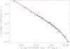 |
Fig. A.1. REFLEX II X-ray luminosity function for the redshift range z = 0 − 0.4. We also show the best-fitting Schechter function and the uncertainty limits of the fit (Böhringer et al. 2014). |
Best-fitting parameters for a Schechter function describing the REFLEX II X-ray luminosity function.
Appendix B: Galaxy clusters tracing the matter distribution
To investigate how well galaxy clusters trace the matter distribution we used the Millennium simulations (Springel et al. 2005). While it is well known that clusters provide a biased account of the fluctuations in the matter density distribution in a statistical analysis such as the two-point-correlation function or the power spectrum, we tested here how well the cluster density correlates with the matter density in individual patches of the Universe. We therefore compared cluster counts in cells to the mean matter density in the cells in the Millennium simulations.
The Millennium simulations are dark-matter-only simulations, which is sufficient for our purpose, since we are looking at very large scales of tens of megaparsecs where baryonic effects play no significant role. The cosmological parameters used for the Millennium study (Ωm = 0.25, σ8 = 0.9, and H0 = 73 km s−1 Mpc−1) are different from our preferred cosmology. Thus the bias is slightly different. However, here we are not interested in calibrating the biasing relation, but we want to demonstrate the method of tracing the matter distribution in spatial patches and to study its uncertainty. For this purpose the difference in the cosmological parameters is not important.
The Millennium simulation has a box size of  Mpc. We selected clusters with a lower mass limit of 0.5 × 10¹⁴ M⊙ finding 5283 such systems in the simulation. We performed two studies: one with a box size of
  Mpc and one with
  Mpc (which correspond to one-eight and one-quarter of the simulation box size, respectively).
The results of the two studies are presented in Fig. B.1. What is shown is the density contrast for clusters as a function of the density contrast in the matter distribution. Therefore, the slope of the relation is equal to the bias. We note that in both cases the distribution of clusters closely traces that of matter. The quantitative result important for the analysis above is the scatter in the relation which was included in the uncertainties of the inferred matter distribution in our analysis. The scatter determined for the two cases is ∼26% for the smaller cells and ∼8% for the larger cells, which is close to the Poisson error. In our analysis we therefore used Poisson uncertainties.
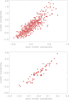 |
Fig. B.1. Cluster over-/under-density with respect to the mean as a function of the matter over-/under-density for counts in cells with a box size of |


Appendix C: Hubble parameter as function of underdensity
We calculated the Hubble constant that should be observed within a local underdensity under the assumption that the underdense region is homogeneous. Justified by Birkhoff’s theorem, we integrated the Friedman equations from initial conditions in the early Universe (z = 500) to the present time for our preferred cosmology and other models with sightly higher or lower densities, and compared their expansion parameters at z = 0. The resulting relation between the underdensity and the increase of the Hubble parameter at present time is shown in Fig. C.1. In the literature one can find approximate formulas for this relation of the underdensity in a local region and the observed Hubble constant, for example by Marra et al. (2013), which agree with our result.
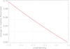 |
Fig. C.1. Change of the Hubble parameter as a function of the underdensity of the region studied. The dotted lines mark the underdensity values of 30 ± 15%. |
All Tables
Best-fitting parameters for a Schechter function describing the REFLEX II X-ray luminosity function.
All Figures
|
Fig. 1. Cluster density distribution as a function of redshift for the CLASSIX galaxy clusters covering the sky at |bII| ≥ 20° for a minimum luminosity of 1042 erg s−1 (0.1–2.4 keV). The density distribution has been normalised by the expected cluster density based on the average luminosity function as explained in Sect. 3. The open square shows the result if the region of the Virgo cluster is excluded from the analysis. |
| In the text | |
|
Fig. 2. Mean X-ray luminosity limit as a function of redshift for the CLASSIX survey. |
| In the text | |
|
Fig. 3. CLASSIX galaxy cluster density distribution as a function of redshift for four different lower X-ray luminosity limits, given in the plot by the parameter xlim in units of 1044 erg s−1. All samples trace the same local density deficit. |
| In the text | |
|
Fig. 4. Sky distribution of the clusters (black dots) and their surface density in the CLASSIX survey at |bII| ≥ 20° smoothed with a Gaussian filter with σ = 10° in the redshift slice z = 0 − 0.04 in equatorial coordinates. The colour coding for the density normalised to the mean is orange: > 2, red: 1 − 2, brown: 0.5 − 1, and dark brown/black: < 0.5. |
| In the text | |
|
Fig. 5. Cluster density distribution as a function of redshift for the REFLEX II survey in the southern sky (open red circles) and the NORAS II survey in the north (filled blue circles) at |bII| ≥ 20°, for a minimum luminosity of 1042 erg s−1 (0.1–2.4 keV). The density distribution has been normalised by the expected cluster density based on the average luminosity function as explained in Sect. 3. |
| In the text | |
|
Fig. 6. Cluster density distribution as a function of redshift in the northern Galactic cap (filled blue circles) and southern Galactic cap (open red circles) at |bII| ≥ 20°, for a minimum luminosity of 1042 erg s−1 (0.1–2.4 keV). The density distribution has been normalised by the expected cluster density based on the average luminosity function as explained in Sect. 3. |
| In the text | |
|
Fig. 7. Sky distribution of the clusters and their surface density in the CLASSIX survey with the extension into the zone of avoidance in equatorial coordinates. The survey is bounded by an interstellar hydrogen column density limit of nH ≤ 2.5 × 1021 cm−2. The white contours show the hydrogen column density boundary of nH = 1.5 × 1021 cm−2. The red lines indicate the Galactic latitudes of |bII|= ± 20°. The yellow dashed line marks the Supergalactic plane and the colour coding is the same as in Fig. 4. |
| In the text | |
|
Fig. 8. Cluster density distribution as a function of redshift in the zone of avoidance at |bII|< 20°. Filled symbols are for the region with a Galactic hydrogen column density of nH < 2.5 × 1021 cm−2 and open symbols for nH < 1.5 × 1021 cm−2. The cluster sample in these region is not complete and therefore the data provide a lower limit. The density distribution has been normalised by the expected cluster density based on the average luminosity function as explained in Sect. 3. |
| In the text | |
|
Fig. 9. Cumulative density distribution of REFLEX II clusters as a function of redshift normalised to the mean for a lower X-ray luminosity limit of LX0 = 5 × 1042 erg s−1 (lower curve with red uncertainty limits). The upper curve with green uncertainty limits shows the inferred dark matter distribution after correcting for the cluster bias. |
| In the text | |
|
Fig. 10. Cumulative density distribution of NORAS II clusters as a function of redshift normalised to the mean for a lower X-ray luminosity limit of LX0 = 5 × 1042 erg s−1 (lower curve with red uncertainty limits). The upper curve with green uncertainty limits shows the inferred dark matter distribution after correcting for the cluster bias. |
| In the text | |
|
Fig. 11. Cumulative density distribution of CLASSIX clusters as a function of redshift normalised to the mean for a lower X-ray luminosity limit of LX0 = 5 × 1042 erg s−1 (lower curve with red uncertainty limits). The upper curve with green uncertainty limits shows the inferred dark matter distribution after correcting for the cluster bias. |
| In the text | |
|
Fig. 12. Sky distribution of the clusters and their surface density in the extended CLASSIX survey in equatorial coordinates. Particular regions marked and labelled in the figure are explained in the text. The red lines mark the Galactic latitudes |bII| ± 20° and the displayed survey region is limited by an interstellar hydrogen column density value of nH ≤ 2.5 × 1021 cm−2. The yellow lines mark the boundaries of regions A to C and the blue lines those of regions D to F. |
| In the text | |
|
Fig. 13. Density distribution of CLASSIX clusters as a function of redshift in the region labelled C in Fig. 12. We find no cluster in the second redshift bin marked by a downward pointing triangle. The galaxy distribution (Whitbourn & Shanks 2014) in the same area is shown by smaller red points with error bars. There is good agreement between both density distributions. |
| In the text | |
|
Fig. 14. Top: density distribution of CLASSIX clusters as a function of redshift in the high-density region in the southern sky, D (red filled circles), and the low-density region, E (blue open circles). Bottom: density distribution of CLASSIX clusters as a function of redshift in the northern high-density region, F. This seems to be one of the densest regions at z ≤ 0.04. |
| In the text | |
|
Fig. A.1. REFLEX II X-ray luminosity function for the redshift range z = 0 − 0.4. We also show the best-fitting Schechter function and the uncertainty limits of the fit (Böhringer et al. 2014). |
| In the text | |
|
Fig. B.1. Cluster over-/under-density with respect to the mean as a function of the matter over-/under-density for counts in cells with a box size of |
| In the text | |
|
Fig. C.1. Change of the Hubble parameter as a function of the underdensity of the region studied. The dotted lines mark the underdensity values of 30 ± 15%. |
| In the text | |
Current usage metrics show cumulative count of Article Views (full-text article views including HTML views, PDF and ePub downloads, according to the available data) and Abstracts Views on Vision4Press platform.
Data correspond to usage on the plateform after 2015. The current usage metrics is available 48-96 hours after online publication and is updated daily on week days.
Initial download of the metrics may take a while.