| Issue |
A&A
Volume 651, July 2021
|
|
|---|---|---|
| Article Number | A105 | |
| Number of page(s) | 18 | |
| Section | Stellar atmospheres | |
| DOI | https://doi.org/10.1051/0004-6361/202040159 | |
| Published online | 27 July 2021 | |
Simultaneous photometric and CARMENES spectroscopic monitoring of fast-rotating M dwarf GJ 3270
Discovery of a post-flare corotating feature
1
Institut für Astrophysik,
Friedrich-Hund-Platz 1,
37077
Göttingen,
Germany
e-mail: This email address is being protected from spambots. You need JavaScript enabled to view it.
2
Max Planck Institute for Solar System Research,
Justus-von-Liebig-Weg 3,
37077
Göttingen,
Germany
3
Hamburger Sternwarte, Universität Hamburg,
Gojenbergsweg 112,
21029
Hamburg,
Germany
4
Instituto de Astrofísica de Canarias,
c/ Vía Láctea s/n,
38205
La Laguna,
Tenerife,
Spain
5
Departamento de Astrofísica, Universidad de La Laguna,
38206
Tenerife,
Spain
6
School of Physics & Astronomy, University of Birmingham,
Edgbaston,
Birmingham
B15 2TT,
UK
7
Instituto de Astrofísica de Andalucía (CSIC),
Glorieta de la Astronomía s/n,
18008
Granada,
Spain
8
Centro de Astrobiología (CSIC-INTA), ESAC, Camino Bajo del Castillo s/n,
28692
Villanueva de la Cañada,
Madrid,
Spain
9
Department of Physics, Ariel University,
Ariel
40700,
Israel
10
Institut de Ciències de l’Espai (ICE, CSIC), Campus UAB, c/ de Can Magrans s/n,
08193
Bellaterra,
Barcelona,
Spain
11
Institut d’Estudis Espacials de Catalunya (IEEC),
08034
Barcelona,
Spain
12
Landessternwarte, Zentrum für Astronomie der Universität Heidelberg,
Königstuhl 12,
69117
Heidelberg,
Germany
13
Department of Earth and Planetary Science, Graduate School of Science, The University of Tokyo,
7-3-1 Hongo, Bunkyo-ku,
Tokyo
113-0033,
Japan
14
Thüringer Landessternwarte Tautenburg,
Sternwarte 5,
07778
Tautenburg,
Germany
15
Max-Planck-Institut für Astronomie,
Königstuhl 17,
69117
Heidelberg,
Germany
16
Departamento de Física de la Tierra y Astrofísica & IPARCOS-UCM (Instituto de Física de Partículas y del Cosmos de la UCM), Facultad de Ciencias Físicas, Universidad Complutense de Madrid,
28040
Madrid,
Spain
17
Komaba Institute for Science, The University of Tokyo,
3-8-1 Komaba,
Meguro,
Tokyo
153-8902,
Japan
18
JST, PRESTO,
3-8-1 Komaba,
Meguro,
Tokyo
153-8902,
Japan
19
Astrobiology Center,
2-21-1 Osawa,
Mitaka,
Tokyo
181-8588,
Japan
20
Centro Astronómico Hispano-Alemán (MPG-CSIC), Observatorio Astronómico de Calar Alto, Sierra de los Filabres,
04550
Gérgal,
Almería,
Spain
21
Department of Physics, University of Warwick,
Gibbet Hill Road,
Coventry
CV4 7AL,
UK
Received:
17
December
2020
Accepted:
23
March
2021
Abstract
Context. Active M dwarfs frequently exhibit large flares, which can pose an existential threat to the habitability of any planet in orbit in addition to making said planets more difficult to detect. M dwarfs do not lose angular momentum as easily as earlier-type stars, which maintain the high levels of stellar activity for far longer. Studying young, fast-rotating M dwarfs is key to understanding their near stellar environment and the evolution of activity.
Aims. We study stellar activity on the fast-rotating M dwarf GJ 3270.
Methods. We analyzed dedicated high cadence, simultaneous, photometric and high-resolution spectroscopic observations obtained with CARMENES of GJ 3270 over 7.7 h, covering a total of eight flares of which two are strong enough to facilitate a detailed analysis. We consult the TESS data, obtained in the month prior to our own observations, to study rotational modulation and to compare the TESS flares to those observed in our campaign.
Results. The TESS data exhibit rotational modulation with a period of 0.37 d. The strongest flare covered by our observing campaign released a total energy of about 3.6 × 1032 erg, putting it close to the superflare regime. This flare is visible in the B,V, r, i, and z photometric bands, which allows us to determine a peak temperature of about 10 000 K. The flare also leaves clear marks in the spectral time series. In particular, we observe an evolving, mainly blue asymmetry in chromospheric lines, which we attribute to a post-flare, corotating feature. To our knowledge this is the first time such a feature has been seen on a star other than our Sun.
Conclusions. Our photometric and spectroscopic time series covers the eruption of a strong flare followed up by a corotating feature analogous to a post-flare arcadal loop on the Sun with a possible failed ejection of material.
Key words: stars: activity / stars: flare / stars: chromospheres / stars: late-type / stars: rotation / stars: individual: GJ 3270
© E.N. Johnson et al. 2021
 Open Access article, published by EDP Sciences, under the terms of the Creative Commons Attribution License (https://creativecommons.org/licenses/by/4.0), which permits unrestricted use, distribution, and reproduction in any medium, provided the original work is properly cited.
Open Access funding provided by Max Planck Society.
1 Introduction
As a result of their ubiquity, low mass, and close-in habitable zones, M dwarfs have garnered the interest of exoplanet surveys hunting Earth-like analogs. Some of these stars, however, are also known to have exceptional levels of stellar activity (Gizis et al. 2000; Khodachenko et al. 2007; Yelle et al. 2008; O’Malley-James & Kaltenegger 2017; Guarcello et al. 2019). These high levels of stellar activity cannot only make planet detection more difficult, but also call into question the habitability of any planets found around these stars (Johnstone et al. 2019; Tilley et al. 2019). The ionizing radiation and high energy particles released can erode or completely strip the atmosphere of an otherwise habitable planet. This process is particularly concerning for planets around M dwarfs because the habitable zone of these stars is much closer in. Particularly energetic events have been proposed as triggers of extinction events on Earth (Lingam & Loeb 2017). Therefore, knowing the frequency, energy, and history of these events on the host star is critical to understanding the habitability potential of a given exoplanet.
Stellar activity manifests itself on our Sun most prominently in the form of sunspots, plages, flares, and coronal mass ejections (CMEs; Strassmeier 1993; Benz & Güdel 2010). Stellar activity is usually more extreme in younger, faster-rotating stars (Appenzeller & Mundt 1989; Kiraga & Stepien 2007; Newton et al. 2016; Guarcello et al. 2019). Additionally the proportion of active to quiet stars in the M spectral type is higher than in other types of stars (West et al. 2008; Reiners et al. 2012; Jeffers et al. 2018). This effect is even more pronounced for late M dwarfs. It has been proposed, for M dwarfs later than ~M 4, that this is due to the geometry of a the magnetic field of a star, which prevents ejection of material and inhibits the magnetic breaking of the star and its transition to a lower activity state (Barnes 2003; Reiners & Mohanty 2012).
While starspots on M dwarfs can often be studied from rotational modulation in photometric time series (Kron 1952; Barnes et al. 2015), the most noticeable feature of stellar activity in either photometry or spectroscopy are stellar flares (Budding 1977). Stellar flares result from a release of energy caused by magnetic reconnection in the upper atmosphere (Hawley & Pettersen 1991; Haisch et al. 1991; Hilton et al. 2010; Benz & Güdel 2010). This reconnection forces free electrons to follow the magnetic field lines into the chromosphere and photosphere. In the chromosphere, the release of X-rays and enhancement in the chromospheric lines is commonly observed. Upward flows of chromospheric material can also occur as heated material rises into the upper atmosphere. This phenomenon is referred to as chromospheric evaporation (Fisher et al. 1985; Abbett & Hawley 1999). The photosphere reacts by extremely rapid increase in brightness in the affected area (impulsive phase) followed by an exponential decay back to pre-flare brightness (decay phase) once the electron bombardment has ceased (Segura et al. 2010). The decay phase may last minutes to hours and in very rare cases days (Osten et al. 2016; Kuerster & Schmitt 1996). Post-flare arcades and additional minor reconnection events are common during this phase (Gopalswamy 2015). In cool stars flares are more noticeable at shorter wavelengths owing to the contrast of the typical temperatures of flares of ~104 K (Kowalski et al. 2018; Fuhrmeister et al. 2018) and the host star of ~103 K. As the flare-affected region cools during the decay phase, this contrast fades, thereby leading to a change in the continuum slope over the course of the flare duration (Segura et al. 2010).
In spectra, flares are usually detected through enhancement of chromospheric lines, particularly the Balmer lines and those of singly ionized calcium (Hawley & Pettersen 1991; Crespo-Chacón et al. 2006; Fuhrmeister et al. 2008; Schmidt et al. 2011; Fuhrmeister et al. 2018). As opposed to the photometric flare signature of a near-immediate peak at the flare onset, spectroscopically observed flares may not have a peak for many tens of minutes into the event (Benz & Güdel 2010). Line profiles of chromospheric lines can also undergo broadening and exhibit both red and blue asymmetries in response to a flare (Fuhrmeister et al. 2018).
Line asymmetries are thought to vary during the course of a flare. However as a consequence of the random nature of observing a stellar flare, the most common detection is through chance observations during a survey. By their very nature these observations only show a moment in time of the progression of the flare. It is therefore difficult to ascertain in which phase an observation catches the flare, making the assignment of a phase to any observed line asymmetry impossible. In general blue asymmetries are assumed to occur in the pre-flare or rise phase and are indicative of chromospheric evaporation or other bulk upward plasma motions. Red asymmetries, on the other hand, are thought to be associated with coronal rain and the decay phase (Fuhrmeister et al. 2018).
The energies of stellar flares can vary dramatically with the magnitude of the flare and wavelength. The most energetic flares can emit 1037 erg in X-rays that can be an order of magnitude more energetic than that observed in visible wavelengths for the same flare (Kuerster & Schmitt 1996). Günther et al. (2020) estimated the bolometric energy of the largest M dwarf flares to be 1036.9 erg. These estimates, however, are usually based on the assumption that the flare is a blackbody, which may not be a good approximation. On the Sun the largest flares are three orders of magnitude lower in X-rays (Kane et al. 2005). The total energy released in the Carrington Event, the most powerful flare yet recorded, was estimated to be ~1033 erg (Aulanier et al. 2013). The smallest solar flares have been reported with energies as low as 1023 erg (Parnell & Jupp 2000).
The largest, longest-lasting solar flares are frequently associated with a CME. The velocity of this ejected mass can vary from 60 to 3200 km s−1 with masses on the order of 1012 kg (Benz & Güdel 2010). While CMEs are relatively easy to detect on our Sun, particularly if they directly impact Earth, they are far more difficult to detect on other stars and none have yet been conclusively identified (Vida et al. 2019a; Leitzinger et al. 2020). This primarily results from their diffuse nature and being outshined by the host star. Therefore, CMEs are easiest to observe in shorter wavelengths where the contrast is the highest. Coronal mass ejections are thought to produce large, asymmetric blue line asymmetries in Balmer lines as detectable indicators (Vida et al. 2019a). If the shift in the asymmetry corresponds to a velocity of at least 10% of the stellar escape velocity, we can be reasonably confident that a CME has occurred. These CMEs are frequently associated with prominence ejections. Munro et al. (1979) found that as much as 70% of solar CMEs have an ejected prominence at their core. It is known that the mass of a prominence depends on the strength of the magnetic field of the host star (Villarreal D’Angelo et al. 2018). M dwarfs are known to have much stronger magnetic fields than the Sun (Shulyak et al. 2019) and thereby can presumably host much larger prominences. Cho et al. (2016) detect a large prominence prior to a flaring event on the Sun using high cadence spectroscopy.
While flaring is fundamentally random in nature, the odds of observing a flare increases when observing the more active fast-rotatingstars due to the rotation-activity relation. The MEarth survey identified a number of stars whose rotational periods are thought to be less than a day (Berta et al. 2012). One of these stars, GJ 3270, is a M 4.5 V star with a v sin i greater than 30 km s−1 and a rotation period shorter than 10 h (e.g., West et al. 2015; Kesseli et al. 2018).
In this paper, we analyze a series of flares that were observed on the ultra-fast-rotating M dwarf GJ 3270, which we observed on 15 December 2018, utilizing high cadence, simultaneous spectroscopy and photometry. In Sect. 2 we provide details on the instruments and the reduction of the data. In Sect. 3 we discuss the stellar parameters of GJ 3270. Section 4 we introduce the methods used to analyze the data. In Sect. 5 we present the results of our analysis, then discuss these results in Sect. 6.
2 Observations and data reduction
We present the instruments and data reduction used in this paper. The simultaneous, ground-based, photometry is discussed first followed by the long-baseline SuperWASP data. We then discuss the TESS data reduction followed up by the spectroscopic data provided by CARMENES.
2.1 Ground-based photometry
We obtained multiband photometry of GJ 3270 simultaneously with the MuSCAT2 instrument, mounted at the 1.52 m Telescopio Carlos Sánchez in the Teide Observatory (Narita et al. 2019), and the T150 and T90 Ritchie-Chrétien telescopes of the Observatorio de Sierra Nevada (SNO). The MuSCAT2 instrument has a field of view (FOV) of 7.4 × 7.4 arcmin. This instrument was designed to carry out multicolor simultaneous photometry. In our run, we used the r (full width at half maximum; FWHM: 1240 Å, henceforth r), i (FWHM: 1303 Å, henceforth i), and zs (FWHM: 2558 Å) bands, which we refer to as r, i, and z bands in the following. The data that we utilized were preprocessed using the MuSCAT2 data pipeline, detailed in Parviainen et al. (2020).
The T150 and T90 telescopes at SNO were used to obtain simultaneous photometry in the Johnson B (FWHM: 781 Å) and V (FWHM: 991 Å) filters. The telescopes are equipped with similar CCD cameras (VersArray 2k × 2k). Their FOVs are 7.9 × 7.9 arcmin2 and 13.2 × 13.2 arcmin2, respectively (Rodríguez et al. 2010). During the readout, we applied 2 × 2 binning for the T150 camera and no binning for the T90 camera.
Each CCD frame was corrected for bias and flat field and, subsequently, light curves were extracted by applying synthetic aperture photometry. All frames cover a number of suitable comparison stars for differential photometry. Different aperture sizes were tested to choose the best size for our observations. The normalization was done by dividing the light curve by its median value. The start time, duration, and exposure times of each photometric run are given in Table 1. Excerpts of the final normalized light curves, showing the two most prominent flaring events, are shown in Fig. 1.
The Super-Wide Angle Search for Planets (SuperWASP, Pollacco et al. 2006) survey is a transiting planet survey conducted from two robotic observatories (located in La Palma, Spain, and Sutherland, South Africa), each with a setup of eight wide-angle cameras. The observations are done through a broadband filter covering 400–700 nm. GJ 3270 was monitored by the SuperWASP program from 2008 to 2014, culminating in ~57 000 observationsover six seasons, each lasting about three months. Data were reduced by the SuperWASP team and detrended using methods designed to preserve variations of astrophysical origin, as detailed in Tamuz et al. (2005). As we utilized SuperWASP data for the sole purpose of analyzing dominant periodicities, associated with the stellar rotation and not for flaring analysis, we filtered the SuperWASP light curves iteratively to remove 4.0σ outliers.
Start time, duration, and exposure time at time of flare of photometric observations. SNO: S, MuSCAT2: M.
2.2 Space-based TESS photometry
GJ 3270 was observed in Sector 5 by the Transiting Exoplanet Survey Satellite (TESS; Ricker et al. 2015) in two-minute cadence mode between 15 November and 11 December 2018. These observations ended five days prior to the beginning of our campaign. We used the TESS light curves available at Mikulski Archive for Space Telescopes. Utilizing the PDCSAP data, we removed thedata points flagged as low-quality by the TESS pipeline (Jenkins et al. 2016) prior to our analysis. The TESS light curve is given in Fig. 2.
2.3 CARMENES spectra
CARMENES1 is a fiber-fed, highly stabilized spectrograph mounted at the Calar Alto 3.5 m telescope. The instrument has a visual (VIS) and near-infrared (NIR) channel, which are operated simultaneously (Quirrenbach et al. 2016). The VIS channel operates between 520and 960 nm and the NIR channel between 960 and 1710 nm at spectral resolutions of 94 600 and 80 400, respectively.
Our observations of GJ 3270 were carried out on 15 December 2018 and comprise 28 VIS and NIR spectra, which each have an exposure time of 15 min. The spectral time series covers a total of 7.7 h. All spectra were reduced using the caracal pipeline, which relies on the flat-relative optimal extraction (Zechmeister et al. 2014; Caballero et al. 2016). In Table A.1, we give the central time of the observations and the duration since the first observation, and assign an observation number, which is used to refer to the spectra in the following.
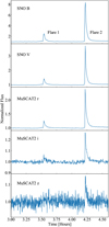 |
Fig. 1 SNO observations normalized light curves in V and B band areshown in the top two panels. The normalized light curves of the MuSCAT2 data, in r, i, and z bands, are represented in the bottom three panels. |
3 Stellar parameters
GJ 3270 has been placed in several young associations. In particular, it was proposed to be a member of the AB Doradus moving group by Bell et al. (2015). Cortés-Contreras et al. (2017) proposed GJ 3270 as a member of the Local Association, also known as the Pleiades moving group (Eggen 1983). These groups range in age from 20 to 300 Myr. The ROSAT All Sky Survey measured X-ray emission to be log (Lx) = 28.3 erg s−1 (Voges et al. 1999). This value is too low for the younger groups but is compatible for those from similar objects in AB Dor. Lithium 6708 Å was not detected in our spectra. This indicates that the age of GJ 3270 must be greater than about 50 Myr (Zickgraf et al. 2006). Therefore our age range for GJ 3270 is 50 Myr to 300 Myr with a most probable age of ~150 Myr as a member of AB Doradus. In color-magnitude diagrams GJ 3270 is not significantly over-luminous (Cifuentes et al. 2020). This indicates that it is nearly, or already on, the main sequence, as is expected for low-mass stars older than 100 Myr. Therefore, we can use main-sequence relations to determine its stellar parameters.
Using multiwavelength photometry from the blue optical to the mid-infrared, Cifuentes et al. (2020) estimate a Teff of 3100 ± 50 K for of GJ 3270. Using magnitude values only from Zacharias et al. (2013) and the color-temperature relations from Cox (2000), Reid & Hawley (2005), and Pecaut & Mamajek (2013), we were able to confirm this value. However, owing the fast rotation and youth of GJ 3270, we assume a conservative ±200 K uncertainty when using Teff in calculations. We chose a PHOENIX model spectra (Husser et al. 2013) with Teff = 3100 K, log g = 5.0, and solar metallicity for our template spectra.
Cifuentes et al. (2020) also estimate the luminosity of GJ 3270 to be 0.00642 ± 0.00003 L⊙. With the mass-luminosity relationship in Eq. (1) (Schweitzer et al. 2019),
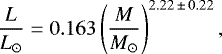 (1)
(1)
we determine the mass to be 0.25 ± 0.07 M⊙, which is consistent with the findings of Cifuentes et al. (2020).
Five days prior to our SNO and MuSCAT2 observations, TESS ended its observation of GJ 3270. We searched forperiodic signals in the combined data set of the TESS, SNO, and MuSCAT2 photometric data using the generalized Lomb–Scargle periodogram (GLS, Zechmeister & Kürster 2009). The resulting power spectrum is shown in Fig. 3. The most significant signal is found at a period of 0.369829 ± 0.0000036 d (frequency ~2.70 d−1), which we interpret as the stellar rotation period and, henceforth, denote it by Prot. The TESS light curve phase-foldedto Prot is shown in Fig 4. We consider the other formally highly significant peak at about 0.1848 d, which is very close to the rotational period reported by West et al. (2015) and Schöfer et al. (2019), a semi-period of the first because its power is about four times lower and nearly half the value of Prot. The West et al. (2015) period determination was based on MEarth data prior to 2011. Interestingly, an analysis of the SuperWASP light curves, which span several seasons, shows an evolution in the dominant periodicity from 0.1849 d before 2011 to 0.3697 d after 2013, as illustrated in Fig. 5.
This evolution of dominant periodicity was previously described in Basri & Nguyen (2018) and Schöfer et al. (2019). They proposed a geometrical solution to the periodicity shifts. The simplest, solution being two spots 180 deg apart on the stellar surface. In Sects. 6.2 and 6.3 we show evidence for two active regions on opposite hemispheresof GJ 3270. These regions, however, are traced using chromospheric activity indicators that are indicative of faculae or plague features more than spots. While we surmise that the periodicity shifts can arise from any bimodal surface, or near surface, heterogeneity that varies in relative strength over time, the driving mechanism is behind this phenomenon remains unclear. We consider this issue in need of further research because it has strong implications on determining whether a radial velocity (RV) signal is a potential close-in planet or stellar activity.
Reiners et al. (2018) report the v sin i of GJ 3270 to be 35.3 ± 3.5 km s−1 and Kesseli et al. (2018) report a v sin i value of 37.3 ± 1.3 km s−1. In this work, we adopt the more conservative estimate by Reiners et al., but we note that using the Kesseli et al. values does not appreciably alter the results of this paper2. Combining the v sin i with the photometric rotation period, Prot, the value for the stellar radius can be constrained as follows:
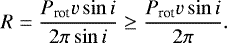 (2)
(2)
This yields a lower radius limit of 0.26 ± 0.05 R⊙, which is consistent with the 0.278 ± 0.009 R⊙ determined by Cifuentes et al. (2020). Out of an abundance of caution we doubled the error bars we had initially calculated owing to the youth of GJ 3270. This radius determination lends support to the conclusion that the 0.1848 d period is a semi-period of the 0.3698 d period.
Adopting the latter radius allows us to estimate the inclination of the stellar rotation axis, which yields a best estimate of 68 ± 15 deg for the inclination and a value of 38 ± 1.2 km s−1 for the equatorial rotation velocity. We present these and other known parameters of GJ 3270 in Table 2.
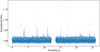 |
Fig. 2 TESS light curve of GJ 3270 from sector 5 observations. At least 22 flares occurred during this time span. Rotation of ~0.3 d can be seen by inspection of the non-flaring light curve. |
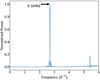 |
Fig. 3 Generalized periodogram of combined TESS and SNO V data. The power level of a 10−3 FAP is 0.0219. |
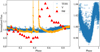 |
Fig. 4 Left: comparison of the phase-folded TESS flare-removed light curve (blue crosses) and SNO V (orange circles) photometric data with CARMENES Hα I∕Ir (red triangles) for flares 1 and 2. The Hα values have been normalized by their median value to properly relate them to the TESS and SNO V values. Right: phase-folded, flare-removed light curve of TESS observations of GJ 3270. |
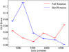 |
Fig. 5 Comparison of the GLS power (Zechmeister & Kürster 2009) of the full- and half-rotation period of GJ 3270 from SuperWASP data. The error bars denote observing seasons from which the GLS periodograms were generated. |
GJ 3270 basic properties.
4 Analysis
In this section we lay out the methods to be used in the analysis of the photometric and spectroscopic data.
4.1 Flareenergy estimation
Our normalized multiband light curves show easily recognizable flare signatures above the underlying photospheric background, but these light curves lack an absolute calibration because no photometric standard stars were available in our FOV. To obtain fluxes and luminosities for the flares, we used a PHOENIX model spectrum (see Sect. 3) as an absolute reference for the photospheric spectrum. We obtained band-specific stellar surface fluxes, fb, by folding the PHOENIX spectrum with the respective filter transmission curves. Multiplication with the stellar surface area (see Sect. 3) then yielded the band-specific photospheric luminosity, Lb, against which the flare is observed.
To study the flare parameters, we set up a light curve model with an exponential form. The free parameters are the flare start time, t0, the peak, lp, and the (exponential) decay time, τ. We also include an offset, which we consider a nuisance parameter. As in particular the TESS light curves show relatively long integration times per photometric data point, we used an oversampled model light curve, which we subsequently binned to the temporal resolution of the respective measurement (e.g., Kipping 2010). We then obtained best-fit parameters with a χ2 minimization. The model provided our normalized photometric light curve lb (ti) at time ti. We obtained flare luminosities, by
 (3)
(3)
The total flare energy in the band, Eb, is obtained by integration of luminosity over the flare period. Assuming an exponential form for the flare light curve, the peak luminosity, Lpeak, b = lp ⋅ Lb, and total flare energy are related to the e-folding time, τb, through
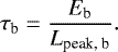 (4)
(4)
We estimate that the relative uncertainty of the total energy amounts to about 10%, primarily caused by the systematic error induced by using the synthetic template.
4.2 Flare model
As we have simultaneous multiband light curves, an estimation of the temperature and the size of the flaring region can be attempted. We first degraded the time resolution of the individual light curves to align their time binning with that of the V -band light curve. To that end, we averaged all r, i, and z-band photometric data points falling into the respective V -band time bin and linearly interpolated the B-band light curve.
In our modeling, we adopt a single blackbody with a temperature Tbb for the flare spectrum. By scaling the flare spectrum with the flare area, Af, and folding with the filter transmission curves, we simulated the response of the different photometric bands.
For each time bin of the rebinned light curve, we estimate values for the blackbody flare temperature, Tbb, and its area, Af, by fitting the model to the five available band fluxes. In the fit, we gave equal weight in the individual light curves by assuming a signal-to-noise ratio (S/N) of 100 for all of them. The fits in the individual time bins are independent, with the exception that we demand that the blackbody temperature does not rise after the flare peak.
4.3 Spectroscopic index definition
We employed the following lines as chromospheric activity indicators: He I D3 λ5877.2 Å (henceforth He I D3), Na D2 λ5891.5 Å (henceforth Na I D2), Na D1 λ5897.5 Å (henceforth Na I D1), Hα λ6564.6 Å, and the Ca II infrared triplet B line at 8500.4 Å (henceforth Ca II IRT). We focused on the latter component because the Ca II IRT A & C lines are closer to the edge of the CCD and subject to greater uncertainty. The He I λ10 830 Å triplet lines are heavily affected by telluric OH emission lines and are, therefore, not suitable for our analysis. The Na D lines also show some telluric contamination, which mainly affects the last hour of our observations because GJ 3270 was low on the horizon, but this does not impede our analysis.
We used the index method as described by Kürster et al. (2003) to quantify the state of the chromospheric indicators. For each line, L, index values, IL, are calculated for all spectra according to
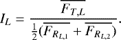 (5)
(5)
In this equation,  denotes the average flux density over a target region, covering the respective line core, and
  and
and  indicate averages over reference regions of pseudo-continuum. We adopted the same width of 5 Å for all regions. Details are given in Table 3.
The relatively broad target regions account for the strong rotational line broadening and additional broadening of the chromospheric line cores during flares. Uncertainties on the index values were obtained by error propagation as follows:
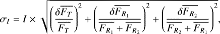 (6)
(6)
where  ,
,  , and
, and  denote the uncertainties of the respective mean, and the line index, L, was dropped for readability. All index values and uncertainties are listed in Table A.2.
To better study the relation between the activity indices, we created a relative index (henceforth I∕Ir) for every line, L, such that
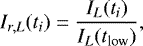 (7)
(7)
where tlow denotes the minimum activity state, corresponding to the spectrum with the lowest observed Hα index value (observation no. 13). This was also the case for all the other activity indicators except for He I D3, which had the first exposure, of our observation period, as its lowest value.
Vacuum wavelength ranges adopted for index definition.
5 Results
We applied the methods discussed in Sect. 4 to the photometric (Sect. 5.1) and spectroscopic (Sect. 5.2) data. In Sect. 5.3 we compared these results with emphasis on timing and energy differences of the effect of the flare in the photometric and spectroscopic data.
5.1 Photometry
We present the results from analyzing the photometric data from SNO and MuSCAT2 (Sect. 5.1.1) and TESS (Sect. 5.1.2). We emphasize the determination of the energy, peak luminosity, and e-folding decay time of the flares. This allows us to determine that the flares that we observed on 15 December 2018 do not differ greatly when compared to the characteristics of the flares TESS observed the month prior.
5.1.1 SNO and MuSCAT2
The light curves in Fig. 1 show two prominent flare-like events at relative times close to 3.6 h (henceforth flare 1) and 4.2 h (henceforth flare 2), of which the latter shows higher peak flux in all bands. At least five weaker flares were observed in the B and V bands, primarily early in the observing run (Fig. 6).
The different exposure times and relative offsets in cadence complicate the determination of the instant of flare onset. We normalized the flare light curves by the peak flux (Fig. 7). This allowed us to identify a 2.6 s window of overlap between the first bins, which consider to show elevated flux due to flaring. Therefore we determined that the onset of flare 2 occurred at UT 15-12-2018 23:47:33 (4.2167 h into the observations, JD 2458468.49135 ±1.3 s), which is consistentwith simultaneous onset in all light curves. While we consider this strong evidence that a simultaneous onset occurred, it does not eliminate the possibility of a delayed onset. We are able to constrain any such delay to a maximum of 25 s between onset in B and onset in z, which would still satisfy the observed light curves.
We applied the methods described in Sect. 4.1 to determine the band energy, peak luminosity, and e-folding decay time. We present these values in Table 4. The results for the z band in flare 1 remain insignificant and are, therefore, not listed in the table. The e-folding decay times are presented in Table 4.
Flaring is generally more pronounced in the bluer bands, which is a consequence of the higher temperature flare spectra contrasting against the cooler stellar spectra (McMillan & Herbst 1991; Rockenfeller et al. 2005). This behavior is also exhibited by flare 2 asshown in Fig. 1. This effect is so pronounced that flare 1 becomes essentially undetectable in the z band. From our best-fit model (see Sect. 4.2) we determine the peak temperature of flare 2 to be ~10 000 ± 1500 K, covering an area of (1.35 ± 0.39) × 1019 cm2. Using the same procedure to calculate the total bolometric luminosity assuming the flare is a blackbody as in Günther et al. (2020) and Shibayama et al. (2013), we estimate the total energy to be (6.3 ± 3.2) × 1032 erg, which is consistent with the sum of B, V, R, i, and z band energies of 3.6 × 1032 erg. This puts flare 2 close to the superflare regime of flares with bolometric energy greater than about 1033 erg (Shibayama et al. 2013).
However, while the model fits well to the peak and early decay phase, it does not reproduce the onset or late decay phase. For the onset we suspect that the issue lies in the aforementioned differences in cadence and exposure and the swift development of the flare. For the late decay phase the parameters become degenerate as the flare-affected region cools and, therefore, are no longer reliable. In our energy calculation we omit these degenerate values but nevertheless we assign a conservative 20% error on the energy estimate.
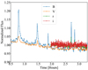 |
Fig. 6 Minorflaring in B, V, r, and i bands that occurred at the beginning of the observation run. |
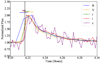 |
Fig. 7 Multiband light curve of flare 2 normalized by peak flare flux. The horizontal bars indicate the integration time of the flare onset observation for each band. Because of the low S/N of the z-band observations, we extended the possible onset time of the flare by an additional exposure. The dashed lines represent the onset window for flare 2 that would satisfy the onset conditions of all the photometric bands. |
Parameters of flares 1 and 2.
5.1.2 TESS
We carried out a search for flares in the TESS light curve. To that end, we classified any photometric excursion as a flare if it peaked more than 3.6σ above the noise (determined by comparing lowest detectable injected flare to the noise background) and consisted of more than three consecutive data points. As the data set is inherently skewed owing to the presence of flares, we used the robust median deviation about the median to estimate the standard deviation of noise (e.g., Rousseeuw & Croux 1993). With our criterion, we identified 22flare events in the 26 day observational period. Our detection threshold for these flare events is ~1031erg. By visual inspection, we determined that 15 of these are isolated events, with a single distinct peak followed by a decay. The remaining seven events were part of three different features consisting of multiple peaks. This occurs when a new event begins prior to the end of the decay phase of the previous event. Whether the events are physically related or are aligned by chance is unclear. Of these seven events, three were rejected from processing. One of these was rejected because if it been an isolated event, it would not have met the 3.6σ criterion. Two others were rejected as their profiles were not able to be fit with an exponential owing to an unusually long decay time or confounding behavior of the continuum. Likewise, one isolated event was rejected for the same issue. The parameters of the remaining flares are given in Table 5.
For individual flare events (IFEs) the peak luminosities, energies, and e-folding decay times were calculated in the same manner as that described in Sect. 4.1 for the SNO and MuSCAT2 data. The flares in the multi-flare events (MFEs) were a bit more complicated in that the decay curves of the individual events were disrupted by the curve of the following event. To estimate the energy, we fit an exponential decay curve based on the peak flux and the data points that existed prior to the next flare occurrence. The same procedure was done for the second and third flare in the sequence, only now subtracting the curve of the prior events. This allowed us to integrate under the curves and get an approximation for the energy output in each flare as if they were individual events. The values of these calculations are given in Table 5.
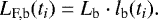
In Fig. 8, we show the flare peak luminosity as a function of flare energy. In comparing the data on the flares observed by TESS to those of flares 1 and 2, we opted to use the values in the i band and r band, added together. We opted to not use the z band as wellbecause only flare 2 was detected in this band.
Isolated and MFEs behave similarly in this diagram, albeit the number of MFEs remain low. While others have identified these MFEs (Tsang et al. 2012; Vida et al. 2019b; Günther et al. 2020), also referred to as outbursts, there is to our knowledge no direct comparison of the parameters of single versus multiple events. Taken in total, however, the data show a statistically significant relation between peak luminosity and energy (p-value of 4.96 × 10⁻⁶).
Parameters of TESS flares.
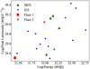 |
Fig. 8 Flare peak flux as a function of total energy for flares 1 and 2 (red square and star, respectively) as well as multiple (green triangles: MFE) and individual flare (blue circles: IFE) events observed by TESS. |
5.2 Spectroscopy
We present the results of analyzing the CARMENES spectroscopic data. The descriptions of the indicators used can be found in Sect. 4.3. First, we present the response of the chromospheric activity indicators (Sect. 5.2.1). These give broad outlines of the activity state of the star at any given time during the observations. Following this, we use the same methodology to examine the asymmetry of the Hα line (Sect. 5.2.2). In Sect. 5.2.3 we show that the blue asymmetry in Hα is caused by blue-shifted emission feature that is strongly correlated with those of the other activity indicators.
5.2.1 Chromospheric index time series
In Fig. 9, we show the time evolution of chromospheric indices. Prior to flare 1 (at about 3.6 h), all the activity indices remained roughly constant with the exception of that of Hα, which showed a decline. Flare 1 did not elicit a strong response from any activity indicators. If not for the photometric signature, flare 1 would have remained undetected. Interestingly, the sodium indices seemed to respond the most, in relation to the response of other indicators, to flare 1 (Fig. 9). In contrast, all indicators showed a pronounced flare signature that is consistent with the timing of photometric flare 2, with a characteristic fast rise and subsequent longer decay phase (Fuhrmeister et al. 2018; Reiners & Basri 2008; Honda et al. 2018; Schmidt et al. 2019).
The most prominent flare 2 response was observed in the Hα line, for which the rise to the peak index value lasted about 45 min. The following decay phase slowed after another 45 min essentially developing a plateau, followed by a moderate linear decay lasting beyond the end of the observations. In comparison to Hα, Ca II IRT reacted the least but reached its peak faster. However, similar to Hα this flare did notfully return to its pre-flare values before the end of observations.
The He I D3 and Na I indices showed similar temporal behavior, marked by a swift (unresolved by 15 min cadence) rise phase followed by a 45 min plateau. After this plateau, the He I D3 and the sodium line indices showed a decay back to pre-flare levels, which appears to proceed the most rapidly in the He I D3 line index. Close to the 6 h mark, the lines showed another enhancement in activity, which coincided with the plateau-like feature seen in the Hα index. The pattern of Ca II IRT decaying slower than He I D3 has been previously noted with other M dwarf flares (Fuhrmeister et al. 2008, 2011).
The Na I D1 and Na I D2 indices showed an apparent increase in activity level after 6.5 h into the observations. This period coincided with increased telluric contamination of the sodium lines (Fig. 14).
Parameters of double Gaussian fit.
5.2.2 Hα wing indices
Flare 2 had effects beyond the core of the Hα line profile with an increase in flux being detected from − 10 to + 5 Å. We show this in Fig. 10 with line fit parameters given in Table 6. Moreover, we quantified the effects in the Hα wings, including asymmetries, by measuring an index on both sides of the core index: the red wing index (RWI) and blue wing index (BWI).
Additionally, we took the index of a broad region that included the line core (Broad Index). The definitions of these indices can be found in Table 3. We plot these new indices along with the original Hα index in Fig. 11.
At the beginning of the observations, the RWI was enhanced over that of the BWI, but by 2 h into the observations the two indices equalized. Neither index reacted to the onset of flare 1. The BWI showed a sharp rise at the onset time of flare 2 followed by an exponential decay with an e-folding time of about 30 min. The RWI also showed a rapid increase at the time of the onset of flare 2 followed by a decay. This decay was interrupted, however, and a secondary rise was detected shortly after 5 h into the observations. The RWI remained elevated over that of the BWI for the remainder of observations. This indicates that the BWI was primarily affected by the events around the flare onset.
Initially the flare onset appeared in the Hα line as a large asymmetry on the blue wing of the line. When subtracting the minimum activity spectrum (Fig. 12) this blue asymmetry is the summation of two features: a narrow and broad component (Fig. 10). We fit a double Gaussian profile to these components, the result of which is given in Table 6.
For the broad component, the fit yielded a shift of − 29.7 km s−1 from the line core and a narrow component shifted by − 25.1 km s−1. This broad component was only strong enough to be fit with a Gaussian at the flare onset, but indices placed even further from the line core than the BWI and RWI indicate that this component lasted for a total of 30 min. This also suggests that the narrow component was limited to the 7 Å nearest the line core as it persisted in the BWI for much longer. The red extreme index did not show as much of an enhancement after 5 h as the RWI, suggesting that the asymmetry detected by the RWI was also confined to within 7 Å of the Hα line core.
The narrow component, represented by the BWI, persisted for at least 90 min while decreasing in strength. This can be seen in the activity minimum subtracted spectrum as the narrow component decreasing in amplitude and shifting toward the line core.
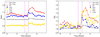 |
Fig. 9 Left: index for Hα (red triangles), He I D3 (blue circles), Na I D2 (yellow squares), Na I D1(orange stars), and Ca II IRT (black crosses) for all observations. Flare 2 occurs at 4.3 h. Hα is scaled down by factor of 2.5. Right: I∕Ir for Hα (red triangles), He I D3 (blue circles), Na I D2 (yellow squares), Na I D1 (orange stars), and Ca II IRT (black crosses) for all observations. Vertical lines in both plots indicate onset times of flares 1 and 2. |
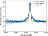 |
Fig. 10 Hα double Gaussian fit for the onset of flare 2. The narrow component (green line) has a shift of − 25.12 km s−1 and the broad component (red line) has a shift of − 29.68 km s−1 from the line core. The combined fit is given by the solid black line. |
5.2.3 Doppler shifted emission
The initial displacement and subsequent shift toward the line core seen in Hα can also be observed in the other activity indicator line profiles (Fig. 13). To more clearly illustrate this, we compiled allof the available spectra for each indicator into a series of “heatmaps” (Fig. 14). These heatmaps show the temporal evolution of the normalized flux density for these lines. The clearest example of the shift is given by the Ca II IRT line because it has the highest S/N. Notably, none of the activity indicator lines have Doppler displacements that exceed the projected rotational velocity of the star. In this picture, the shift in Hα is actually the least obvious owing to the preexisting emission in the line core.
By subtracting the minimum activity spectrum, we can generate a set of residual spectra in which deviations from the quasi-quiescent state can be analyzed. To these residual spectra we fit a Gaussian profile, thereby determining the Doppler displacement from the line core (Fig. 15).
All of the Doppler shift values at the onset of flare 2 are between − 27 km s−1 and − 21 km s−1. The flare onset values of the Hα single Gaussian fit are comparable to the results of the narrow component in the double Gaussian fit.
Prior to flare 1, the Gaussian fits to the Hα and He I D3 residual spectra show predominantly redshifted values, whereas the sodium residuals are either neutral or blueshifted. We attribute these, along with the sporadic shifts exhibited by the sodium lines, to the low amplitude of the signals, telluric interference, and systematic uncertainty caused by the selection of the minimum activity spectrum.
As the onset of flare 1 approached, the Hα residuals became increasingly redshifted. At the onset of flare 1 the Hα shift decreased almost to neutrality and He I D3 appeared blueshifted. After the onset of flare 1 but prior to flare 2 Hα, He I D3, and the sodium lines all appeared blueshifted with a shift of between − 20 and − 10 km s−1. After the onset of flare 2 the shifts of all chromospheric residuals were strongly correlated. Over the subsequent ~2 h, the residuals shifted toward longer wavelengths. Formally, the He I D3 residual emission was the first to return to its rest wavelength and then became increasingly redshifted. Shortly after followed the shifts of the residual Hα and Ca II IRT line cores. For the sodium lines the return to neutrality could not be observed, probably because of telluric interference.
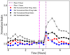 |
Fig. 11 Hα red (RWI) and blue (BWI) wing indices. Hα I∕Ir and broad index are shown in gray and black, respectively. The vertical lines indicate onset times of flares 1 and 2. |
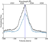 |
Fig. 12 Hα at flare onset (solid black, observation 17) and at activity minimum (solid gray, observation 13). The dashed vertical line indicates the rest wavelength. |
5.3 Spectroscopy versus photometry
In Fig. 4 we juxtapose the phase-folded TESS light curve (with flare events subtracted) with the SNO V band light curve and the Hα index time series; the latter two are scaled. The Hα index data shows a decline prior to flare 2.
Similar behavior is exhibited by our B, V, r band light curves, but it is not detectable in the i and z bands, possibly owing to poorer S/N (Fig. 1). Although the TESS light curve was not taken simultaneously, the narrow gap of only about four days, combined with the relative stability of the rotational signal during the TESS observing window, suggests that the source of the decline in Fig. 4 is rotational variability. This rotational variability is likely caused by corotating active regions, which is also consistent with the effect being more pronounced at shorter wavelengths. This implies that the modulation of the Hα index prior to flare 2 is also, primarily, driven by rotational effects.
The decay times of the activity indicators for flare 2 are, at a minimum, two times longer than those observed in the photometric bands. The e-folding duration of Hα, for instance, is ~3000 s, whereas the longest e-folding duration of a photometric indicator is 1320 s and nearly exponential in nature. The decay phase of Hα appears to be complex with an initial exponential decay followed by a plateau and a later linear decay that lasts until the end of observations. Since the non-exponential decay phase of Hα occurred over a period of time when the photometric flare had already returned to quiescent level, the transition between the phases in the activity indicators is likely due to phenomena that affected the chromosphere but not the photosphere.
Table 7 shows the energies involved for each activity indicator used in this study. Hα, one of the principal cooling lines of the chromosphere, puts out an energy equivalent to ~22% of the r band. However it takes Hα 30 times as long to emit that energy. This contrast in the rate of output between Hα and the r band is clear when looking at the peak luminosity. The photometric value is 148 times larger than the Hα spectroscopic value. The other spectroscopic indicators have similar ratios to the photometric bands in which they occur. The activity indicators (He I D3 and the sodium lines) in the V band are slightly more contrasted (2.5% of the energy output of the V band) as a consequence of the higher temperature of the flare material in comparison to the photospheric background.
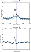 |
Fig. 13 Flare emission from the He I D3 (top) and Ca II IRT lines (bottom) during flare onset (solid black, observation 17), activity minimum spectra (solid gray, observation 13). The dashed vertical line indicates the rest wavelength. |
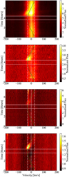 |
Fig. 14 From top to bottom: Hα, He I D3, Ca II IRT, and Na I D2 flux density evolution during our observing run. The central dashed line indicates the nominal rest-frame wavelength and the outer two dash-dotted lines denote the maximum Doppler shift for a corotating object at 43 deg latitude (28.6 km s−1). The green line represents the expected Doppler shift of such an object if it were to emerge onto the blue limb of the disk 3.72 h into the observation run. Horizontal solid white lines indicate onset times of flares 1 and 2. |
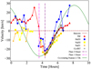 |
Fig. 15 Doppler shift of excess flare emission of the line cores. The missing data points indicate that a Gaussian fit was impossible, which causes the gap at about 3 h, where the minimum activity spectrum is located. All of the activity indicators shift to the blue before the flare onset (noted by vertical dotted line). Green line represents the expected Doppler shift of such an object, at 43 deg latitude, if it were to emerge onto the blue limb of the disk 3.72 h into the observation run. |
Indicator energies for flare 2.
6 Discussion
We present our interpretation and extrapolation of the data above. In Sect. 6.1 we compare the flares observed with SNO and TESS to other flaring M dwarfs. In Sect. 6.2 we interpret the Doppler shifts of the activity indicators as evidence for a corotating feature and isolate the location of it to a latitude of43 deg and a longitude of –70 deg. In Sect. 6.3 we look at the beginning of the observations when sustained minor flaring is associated with a persistent redshift in the Hα line. We find that the data are consistent with an active region, separate from that of flare 2, which was in the process of rotating off the observable disk at that time. In Sect. 6.4 we look at evidence for rotational modulation and find that our data are consistent with Hα being rotationally modulated. Additionally we discuss the Doppler shifts of the activity indicators and find that both major flares likely originate from a similar location on the stellar surface. Additionally, the red excess seen in the Hα wing index is consistently elevated, suggesting ejected material reentering the lower atmosphere. We then compare, in Sect. 6.5, the response of the activity indicators to flares 1 and 2. We present a series of possible scenarios as to why there was such a difference in reaction to the two events. Lastly, we explore the possibility of a CME being associated with the blue asymmetry of flare 2. We find, however, that our data do not support any successful mass ejection of material, but there is some evidence for a failed ejection that later reenters the lower atmosphere causing a disruption to the chromospheric indices.
6.1 Flaring rates and energies
Given the TESS observation period and the observed flare count we calculate a flare rate of 0.818 flares per day. The sum of their decay times was 5,221 s for a duty cycle (time flaring divided by non-flaring time) of 0.23%. Figure 8 shows that flare 1 and 2, which we covered with multiband, ground-based photometry, have similar energies and peak luminosities as the TESS flares observed the month prior. There may be a small separation between high energy, long-duration flares, of which flare 2 is a member, and lower energy flares, of which flare 1 is a member. Whether this gap corresponds to some physical property or mechanism remains speculative.
Vida et al. (2019b), using TESS, measure a flare rate of 1.49 per day on Proxima Centauri with a duty cycle of 7.2%. The average energy output of the 72 events observed on Proxima Centauri is 11.5 × 1030 erg while the average for our observations is 17.8 × 1031 erg, that is, about an order of magnitude more, which is in line with a higher cadence and duty cycle for the events identified on Proxima Centauri. In a larger study of flares observed by TESS, Günther et al. (2020) find that for M dwarfs, with rotation periods <0.3 d, the flare frequency was between 0.1 and 0.5 per day. In a similar study with Sloan Digital Sky Survey, Hilton et al. (2010) find that for M0 to M1 dwarfs the flare duty cycle was 0.02% but went up to 3% for M dwarfs M7 to M9. Although direct comparisons remain difficult owing to different sensitivities and flare detection methodology, our findings are generally consistent with those in comparable stars.
6.2 Localization of flare 2 region
With the information on the Doppler shifts of the chromospheric lines, we can estimate the latitude and longitude of the flaring region. The (rotational) RV (t) of a surface element as a function of time, Δt, and stellar latitude, ϕ, is given by
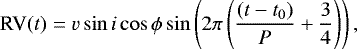 (8)
(8)
where v sin i is the projected equatorial rotation speed, P is the stellar rotation period, and t0 is the instance of minimum RV. For a large inclination, this corresponds well to the instant of appearance of a feature at the limb.
We fit the expression in Eq. (8) to the Hα, He I D3, Na I D1, and Ca II IRT shifts of observations no. 18–22, treating ϕ and t0 as free parameters. In this way, we obtained a latitude of 43 ± 10 deg and a value of 3.73 ± 0.12 h for t0, where the error is estimated using the jackknife method (e.g., Efron & Stein 1981). We did not use the two observations during and after flare onset as these are the most likely to be contaminated by radial bulk motions, as indicated in Fig. 11.
Given the onset time of flare 2, we estimate that the flare started 70 ± 5 deg from the center of the disk. At this instance, Eq. (8) yields a shift of − 26 ± 4 km s−1, which agrees well with the observed RV shift.
The agreement of these two values indicates that the majority of the blueshift of the narrow components originates from the displacement of the active region from the center of the disk and the resulting rotational RV shift rather than bulk motions of flaring material (Figs. 14 and 15). It is likely that the bulk motions are better represented by the broad component featured in Fig. 10. The observed data and the corotating aspect are similar to an active region with post-flare arcadal loops on our Sun.
6.3 Minor flares
Prior to flare 1, Fig. 15 shows that the Hα line is shifted to the red. These redshifts coincide with a series of small flare-like events (Fig. 6). Concurrently with these small flares, the wing index measurement (Fig. 11) of Hα shows an enhancement in the red wing over that of the blue wing. While there are multiple situations in which chromospheric lines can exhibit asymmetries, these red wing enhancements are frequently associated with coronal rain in which the down-falling material emits Hα as it heats up upon reentry of the lower atmosphere (Fuhrmeister et al. 2018).
Starting at two hours into the observation, this redward shift quickly ascends from +10 km s−1 to a peak of +26 km s−1 within about one hour. This maximum occurs just after the last of the minor flare-like events. It is immediately followed by the activity minimum spectrum and for the rest of the observing run there are no further small flare events. For the rest of our observations, the Hα velocity shift value never again reaches the 10 km s−1 value. Additionally the slope of the increasing redshift of the Hα asymmetry is consistentwith a corotating feature. This implies that these minor flares and increasing red asymmetry may be due to an active region moving over the limb of the star just prior to or concurrent with the activity minimum observation. Unfortunately, without data spanning multiple rotation periods, we could not confirm this. We can, however, conclusively rule out any association of the minor flares with flare 1 and 2. If the minor flares were part of the same active region as flare 1 and 2, then they would have occurred while the active region was on the far side of the star and therefore unobservable.
When comparing the minor flaring across photometric bands (Fig. 6), the minor flares are only discernible at short wavelengths (B and V specifically). In the longer wavelength ranges they become indistinguishable from the background. Therefore, if further work is to be done to disentangle possible rotation modulation of Hα from the effect of minor flaring (bulk vertical motion; i.e., coronal rain), it should be done with high cadence, simultaneous spectroscopic and photometric (B and V) observations.
6.4 Rotational modulation and doppler shifts of activity indicators
In Fig. 4, the trend of Hα in the first halfof the observing run is similar, if more exaggerated, to that of the light curve of TESS, suggesting that the Hα index is modulated by rotation. However owing to the onset of flare 2 in the second half of the data set we could not confirm this. There also exists the possibility that Hα index has a periodicity twice that of the rotational period of the star as seen in other active M dwarfs (Schöfer et al. 2019).
An alternative scenario for the pre-flare absorption dip in Hα is supplied by Jardine et al. (2020). They argue that rapidly rotating and young (<800 Myr) stars (such as GJ 3270) are prone to having slingshot prominences. Slingshot prominences are comprised of trapped, cool, gas and appear as absorption transients in Hα. Slingshot prominences are thought to be most common around zero age main-sequence stars (Jardine et al. 2020; Cang et al. 2020). If such a prominence was present prior to flare 2, it was likely disrupted or ejected by that flare because no similarly sized absorption transients are seen for the rest of our observational period. Whether this absorption feature in Hα is due to a prominence or the rotational modulation of Hα is unclear.
For two hours after flare 1 (this time frame includes flare 2) all indicators are closely correlated (Fig. 15). This suggests that flare 1 and 2 are related and likely originate from the same active region. Therefore, given the determined onset position of flare 2, flare 1 would have occurred at or just over the limb of the star.
After flare 2, the Doppler shifts are consistent with a corotating feature, as detailed in Sect. 6.2. At ~6 h into the observations, all of the Doppler shifts of the activity indicators have returned to their line cores and from this point forward become redshifted (Fig. 15). Simultaneously, the activity indicator Doppler shifts diverge from that expected of a corotating feature, suggesting that the post-flare effects in the active region have subsided or are no longer the dominant feature of activity on the disk. Additionally, all the activity indices increase except for Hα, which halts its decay and plateaus for ~45 min (Fig. 9). The wing index (Fig. 11) shows a larger red enhancement at this time than it did during the period of minor flaring. We find these data are consistent with a period of coronal rain, possibly the result of material partially ejected during the onset of flare 2, returning to the star.
Enhancement factor of flare 2 from flare 1 by photometric band.
6.5 Comparison of flare 1 and 2
While the position of flare 2 can be calculated by its after effects, flare 1 is considerably less intense (Table 8, Fig. 1) and has no discernible after effects. We must therefore infer its relation to flare 2.
Just prior to flare 1, the Hα line had reached its maximum redshift value of ~25 km s−1 (Fig. 15). We previously surmised that this may be the signature of an active region ~30 min from going over the limb of the star. At the onset of flare 1, all Doppler shifts of the activity indicators shift towardthe blue. After flare 1, these shifts increase until the maximum blueshift occurs at the onset of flare 2. The Doppler shifts of all the activity indicators are well correlated from flare 1 onset to ~90 min after flare 2onset, indicating that the source of this shift is the dominant chromospheric feature on the star.
The calculated location of the active region that spawned flare 2 at the time of the onset of flare 2 is 70 ± 5 deg from disk center. It would have taken this active region ~30 ± 8 min to arrive at this location from the limb. The timing uncertainty and longer visibility of higher latitudes inclined toward the observer allow that flare 1 originated from the same active region as flare 2. If this active region were the source of flare 1 then flare 1 would have occurred at or near the limb of the star. That we did not see the full blueshifted value of this active region, at that time, could have been due to either a lack of a strong signal or possibly to residual, contaminating effects of the other active region moving over the far limb. This would have been the same active region from whence the minor flares had occurred earlier in the observation period.
This positional argument is supported by the response of the activity indicators (Fig. 9). We conservatively took the flare 2 onset values for I∕Ir and divided them by the V -band flare 2 over flare 1 enhancement (2.6, Table 8) giving us a list of expected activity indicator values for the response to flare 1 if it were proportional to flare 2 (Table 9). This allowed us to compare the expected with the observed indicator values of flare 1. We found that Na I D2, Na I D1, and Ca II IRT responded to flare 1 in proportion to their response to flare 2. Hα and He I D3 however, did not. Both of these indicators were somewhat weaker in flare 1 than would be expected. A possible explanation for this is preferential absorption.
Preferential absorption could arise from an extended light path through the mid-upper atmosphere in which Hα and He I D3 form. In these regions the temperatures are too hot for the ground states of the sodium and calcium lines, thereby allowing the Na I D2, Na I D1, and Ca II IRT lines through unhindered whilst absorbing some of the Hα and He I D3. This extended path would be expected for a source near the limb of the star. While we cannot say for certain that flare 1 occurred on the limb or that it is associated with flare 2, we find the evidence for this case plausible. In this case the observed differences in activity indicator response between flare 1 and 2 would be due to a viewing angle effect.
Expected vs. observed activity indicator response to flare 1.
6.6 Ejection of material
In our observations we do see a large blue asymmetry that has a broad, asymmetric component. This indicates that some bulk plasma motion was occurring during our observations. However the velocity of these plasma motions was at most 30 km s−1, which is only 5% of the escape velocity. Additionally if this material originated from the same active region as the narrow component then it should also have a ~25 km s−1 blueshift due to rotation. We therefore conclude that the detected bulk plasma motions did not result in a CME. However, as we already noted in Sect. 5.2, about 90 min after the onset of flare 2 there was a change in the decay trend of all chromospheric activity indicators into an increasing trend (except for Hα which halts its decay and enters a plateau for ~45 min). During this time the red wing enhancement is at its peak, superseding that of the earlier flaring period. This would indicate, with the assumption that this red wing enhancement is due to an increase in coronal rain, that a considerable amount of material is falling through the chromosphere. During this same time period there were no indications in the photometric data of further flaring activity. We find our data consistent for either a failed loop ejection or a failed CME. In this scenario material from this event rises into the upper atmosphere before raining down and releasing the kinetic energy into the chromosphere, thereby triggering the increase in activity that we observe.
7 Conclusions
We report a series of flares, including a large flare that was followed by a corotating feature, on the ultra-fast-rotating M4.5 V star GJ 3270. We analyzed 27 spectra taken with CARMENES on 15 December 2018. Simultaneous to these observations, photometric observations out in B and V bands from Sierra Nevada and observations in the r, i, and z bands by MuSCAT2 from Teide were carried out. Just prior to our ground-based observations, TESS monitored GJ 3270 for 26 d in a row.
Early in the CARMENES+SNO+MuSCAT2 observing period, a series of minor flaring events were observed along with associated red asymmetriesin the Hα line. This is consistent with the interpretation that these flares were inducing coronal rain. Just prior to the cessation of minor flaring, these red asymmetries increased to the point that the Doppler shift of the residual flux in the Hα had nearly reached the v sin i of the star. No further minor flares were detected for the rest of the observation period. This is consistent with the interpretation that an active region was rotating off the observable disk.
A flare that was larger than those seen during the earlier period of minor flaring occurred 45 min later. This flare (flare 1) had an unusual reaction from the chromospheric activity indicators. Typically Hα is the most sensitive line in flaring situations. In this case, however, the sodium D lines appeared to be the most sensitive followed by He I D3. This unusual reaction coupled with the location of the next, larger flare (flare 2) suggests that flare 1 occurred at or just over the limb of the star. This difference in reaction of the activity indicators, coupled with the position of the flare, can be due to a number of different scenarios. While preferential absorption through a light path containing more stellar atmosphere is a likely explanation, more such situations would have to be observed to come to any firm conclusions.
Flare 2 had energies on the order of 1032 erg s−1. This is comparable to the events detected during the TESS observation period. The most noticeable feature of flare 2 is the strong blue asymmetry in Hα that persisted for ~90 min. At flare onset this asymmetry could be separated into a narrow component and a broad component. The broad component was ~15 Å wide, asymmetric and blueshifted by 30 km s−1 from the line core. This broad component was visually evident only at the flare onset and may have persisted into the next exposure at a minimal level for a total duration of ~30 min. We associate this broad component as indicative of bulk plasma motion. The narrow component was blueshifted by 25.9 km s−1 from the line core. This component is what persisted for the ~90 min for which the blue asymmetry was observed. In other activity indicators (sodium D lines, He I D3, Ca II IRT) an emission peak was observed that is blueshifted by ~25 km s−1 as well. These features then proceeded, well correlated to one another, to shift toward the line core over the subsequent 90 min, while the amplitude of the shifting component decreased. The rate of this shift is consistent with a corotating surface feature that originates at ~65 deg away from disk center with a latitude of ~40 deg. To our knowledge this is the first time such a feature has been observed on an M dwarf. The data are consistent with the solar analogy of an active region experiencing arcadal loops.
Approximately 6 h into the observations and 2 h after flare 2 onset, an increase in chromospheric activity indicators occurred. Associated with this increase was also an elevated period of red asymmetries associated with many of the activity lines. These red asymmetries were larger than those observed earlier during the period of minor flaring. During this same time period, however, no flaring activity was detected in any of the photometric bands. Given that bulk plasma motions were detected during the onset of flare 2, these data are consistent with a period of intense coronal rain, possibly resulting from the reentry of ejected material.
We conclude that the main phenomenon behind our observations was a corotating feature analogous to an active region with arcadal loops. Beyond that, while we have not conclusively shown that a failed CME occurred or that flare regions have a temperature stratification, we have seen sufficient suggestive evidence to warrant further simultaneous, spectroscopic, and photometric observations of fast-rotating M dwarfs.
Acknowledgements
This project was funded principally by the Deutsche Forschungsgemeinschaft through the Major Research Instrumentation Programme and Research Unit FOR2544 “Blue Planets around Red Stars”. CARMENES is an instrument at the Centro Astronómico Hispano-Alemán (CAHA) at Calar Alto (Almería, Spain), operated jointly by the Junta de Andalucía and the Instituto de Astrofísica de Andalucía (CSIC). The authors wish to express their sincere thanks to all members of the Calar Alto staff for their expert support of the instrument and telescope operation. CARMENES was funded by the Max-Planck-Gesellschaft (MPG), the Consejo Superior de Investigaciones Científicas (CSIC), the Ministerio de Economía y Competitividad (MINECO) and the European Regional Development Fund (ERDF) through projects FICTS-2011-02, ICTS-2017-07-CAHA-4, and CAHA16-CE-3978, and the members of the CARMENES Consortium (Max-Planck-Institut für Astronomie, Instituto de Astrofísica de Andalucía, Landessternwarte Königstuhl, Institut de Ciències de l’Espai, Institut für Astrophysik Göttingen, Universidad Complutense de Madrid, Thüringer Landessternwarte Tautenburg, Instituto de Astrofísica de Canarias, Hamburger Sternwarte, Centro de Astrobiología and Centro Astronómico Hispano-Alemán), with additional contributions by the MINECO, the Klaus Tschira Stiftung, the states of Baden-Württemberg and Niedersachsen and by the Junta de Andalucía. We acknowledgefinancial support from the Agencia Estatal de Investigación of the Ministerio de Ciencia, Innovación y Universidades and the ERDF through projects PID2019-109522GB-C5[1:4]/AEI/10.13039/501100011033 and PGC2018-098153-B-C33 and the Centre of Excellence “Severo Ochoa” and “María de Maeztu” awards to the Instituto de Astrofísicade Canarias (SEV-2015-0548), Instituto de Astrofísica de Andalucía (SEV-2017-0709), and Centro de Astrobiología (MDM-2017-0737), the Generalitat de Catalunya/CERCA programme, JSPS KAKENHI via grants JP18H01265 and JP18H05439, and JST PRESTO via grant JPMJPR1775. This work was based on data from the CARMENES data archive at CAB (CSIC-INTA). Data were partly collected with the 150 cm and 90 cm telescopes at the Observatorio de Sierra Nevada (SNO) operated by the Instituto de Astrofífica de Andalucía (IAA-CSIC). This article is based on observations made with the MuSCAT2 instrument, developed by ABC, at Telescopio Carlos Sánchez operated on the island of Tenerife by the IAC in the Spanish Observatorio del Teide.
Appendix A Additional tables
CARMENES observations log.
Activity indicator index values.
Hα wing index values.
References
- Abbett, W. P., & Hawley, S. L. 1999, ApJ, 521, 906 [NASA ADS] [CrossRef] [Google Scholar]
- Appenzeller, I., & Mundt, R. 1989, A&ARv, 1, 291 [NASA ADS] [CrossRef] [Google Scholar]
- Aulanier, G., Démoulin, P., Schrijver, C. J., et al. 2013, A&A, 549, A66 [NASA ADS] [CrossRef] [EDP Sciences] [Google Scholar]
- Barnes, S. A. 2003, ApJ, 586, 464 [NASA ADS] [CrossRef] [Google Scholar]
- Barnes, J., Jeffers, S., Jones, H., et al. 2015, ApJ, 812, 1 [NASA ADS] [CrossRef] [Google Scholar]
- Basri, G., & Nguyen, H. T. 2018, ApJ, 863, 190 [NASA ADS] [CrossRef] [Google Scholar]
- Bell, C. P. M., Mamajek, E. E., & Naylor, T. 2015, MNRAS, 454, 593 [NASA ADS] [CrossRef] [Google Scholar]
- Benz, A. O., & Güdel, M. 2010, ARA&A, 48, 241 [NASA ADS] [CrossRef] [Google Scholar]
- Berta, Z. K., Irwin, J., Charbonneau, D., Burke, C. J., & Falco, E. E. 2012, AJ, 144, 145 [NASA ADS] [CrossRef] [Google Scholar]
- Budding, E. 1977, Ap&SS, 48, 207 [NASA ADS] [CrossRef] [Google Scholar]
- Caballero, J. A., Cortés-Contreras, M., Alonso-Floriano, F. J., et al. 2016, in 19th Cambridge Workshop on Cool Stars, Stellar Systems, and the Sun (CS19), 148 [Google Scholar]
- Caballero, J. A., Guàrdia, J., del Fresno, M. L., et al. 2016, SPIE, 9910, 110 [Google Scholar]
- Cang, T. Q., Petit, P., Donati, J. F., et al. 2020, A&A, 643, A39 [CrossRef] [EDP Sciences] [Google Scholar]
- Cho, K., Lee, J., Chae, J., et al. 2016, Sol. Phys., 291, 859 [NASA ADS] [CrossRef] [Google Scholar]
- Cifuentes, C., Caballero, J. A., Cortés-Contreras, M., et al. 2020, A&A, 642, A115 [NASA ADS] [CrossRef] [EDP Sciences] [Google Scholar]
- Cortés-Contreras, M., Béjar, V. J. S., Caballero, J. A., et al. 2017, A&A, 597, A47 [NASA ADS] [CrossRef] [EDP Sciences] [Google Scholar]
- Cox, A. N. 2000, Allen’s Astrophysical Quantities (Berlin: Springer) [Google Scholar]
- Crespo-Chacón, I., Montes, D., García-Alvarez, D., et al. 2006, A&A, 452, 987 [NASA ADS] [CrossRef] [EDP Sciences] [Google Scholar]
- Efron, B., & Stein, C. 1981, Ann. Stat., 9, 586 [CrossRef] [MathSciNet] [Google Scholar]
- Eggen, O. J. 1983, MNRAS, 204, 377 [NASA ADS] [CrossRef] [Google Scholar]
- Fisher, G. H., Canfield, R. C., & McClymont, A. N. 1985, ApJ, 289, 425 [NASA ADS] [CrossRef] [Google Scholar]
- Fuhrmeister, B., Liefke, C., Schmitt, J. H. M. M., & Reiners, A. 2008, A&A, 487, 293 [NASA ADS] [CrossRef] [EDP Sciences] [Google Scholar]
- Fuhrmeister, B., Lalitha, S., Poppenhaeger, K., et al. 2011, A&A, 534, A133 [NASA ADS] [CrossRef] [EDP Sciences] [Google Scholar]
- Fuhrmeister, B., Czesla, S., Schmitt, J. H. M. M., et al. 2018, A&A, 615, A14 [NASA ADS] [CrossRef] [EDP Sciences] [Google Scholar]
- Gaia Collaboration (Brown, A. G. A., et al.) 2018, A&A, 616, A1 [NASA ADS] [CrossRef] [EDP Sciences] [Google Scholar]
- Gizis, J. E., Monet, D. G., Reid, I. N., et al. 2000, AJ, 120, 1085 [NASA ADS] [CrossRef] [Google Scholar]
- Gopalswamy, N. 2015, Astrophys. Space Sci. Lib., 415, 381 [Google Scholar]
- Guarcello, M. G., Micela, G., Sciortino, S., et al. 2019, A&A, 622, A210 [NASA ADS] [CrossRef] [EDP Sciences] [Google Scholar]
- Günther, M. N., Zhan, Z., Seager, S., et al. 2020, AJ, 159, 60 [CrossRef] [Google Scholar]
- Haisch, B., Strong, K. T., & Rodono, M. 1991, ARA&A, 29, 275 [NASA ADS] [CrossRef] [Google Scholar]
- Hawley, S. L., & Pettersen, B. R. 1991, ApJ, 378, 725 [NASA ADS] [CrossRef] [Google Scholar]
- Hawley, S. L., Gizis, J. E., & Reid, I. N. 1996, AJ, 112, 2799 [NASA ADS] [CrossRef] [Google Scholar]
- Hilton, E. J., West, A. A., Hawley, S. L., & Kowalski, A. F. 2010, AJ, 140, 1402 [NASA ADS] [CrossRef] [Google Scholar]
- Honda, S., Notsu, Y., Namekata, K., et al. 2018, PASJ, 70, 62 [Google Scholar]
- Husser, T. O., Wende-von Berg, S., Dreizler, S., et al. 2013, A&A, 553, A6 [NASA ADS] [CrossRef] [EDP Sciences] [Google Scholar]
- Jardine, M., Collier Cameron, A., Donati, J. F., & Hussain, G. A. J. 2020, MNRAS, 491, 4076 [Google Scholar]
- Jeffers, S. V., Schöfer, P., Lamert, A., et al. 2018, A&A, 614, A76 [NASA ADS] [CrossRef] [EDP Sciences] [Google Scholar]
- Jenkins, J. M., Twicken, J. D., McCauliff, S., et al. 2016, SPIE Conf. Ser., 9913, 99133E [Google Scholar]
- Johnstone, C. P., Khodachenko, M. L., Lüftinger, T., et al. 2019, A&A, 624, L10 [NASA ADS] [CrossRef] [EDP Sciences] [Google Scholar]
- Kane, S. R., McTiernan, J. M., & Hurley, K. 2005, A&A, 433, 1133 [NASA ADS] [CrossRef] [EDP Sciences] [Google Scholar]
- Kesseli, A. Y., Muirhead, P. S., Mann, A. W., & Mace, G. 2018, AJ, 155, 225 [NASA ADS] [CrossRef] [Google Scholar]
- Khodachenko, M. L., Terrada, N., Lammer, H., et al. 2007, European Planet. Sci. Cong. 2007, 561 [Google Scholar]
- Kipping, D. M. 2010, MNRAS, 408, 1758 [NASA ADS] [CrossRef] [Google Scholar]
- Kiraga, M., & Stepien, K. 2007, Acta Astron., 57, 149 [NASA ADS] [Google Scholar]
- Kowalski, A. F., Mathioudakis, M., & Hawley, S. L. 2018, in 20th Cambridge Workshop on Cool Stars, Stellar Systems and the Sun, 42 [Google Scholar]
- Kron, G. E. 1952, ApJ, 115, 301 [NASA ADS] [CrossRef] [Google Scholar]
- Kuerster, M., & Schmitt, J. H. M. M. 1996, A&A, 311, 211 [Google Scholar]
- Kürster, M., Endl, M., Rouesnel, F., et al. 2003, A&A, 403, 1077 [NASA ADS] [CrossRef] [EDP Sciences] [Google Scholar]
- Leitzinger, M., Odert, P., Greimel, R., et al. 2020, MNRAS, 493, 4570 [Google Scholar]
- Lingam, M., & Loeb, A. 2017, ApJ, 848, 41 [NASA ADS] [CrossRef] [Google Scholar]
- McMillan, J. D., & Herbst, W. 1991, AJ, 101, 1788 [Google Scholar]
- Munro, R. H., Gosling, J. T., Hildner, E., et al. 1979, Sol. Phys., 61, 201 [Google Scholar]
- Narita, N., Fukui, A., Kusakabe, N., et al. 2019, J. Astron. Teles. Instrum. Syst., 5, 015001 [Google Scholar]
- Newton, E. R., Irwin, J., Charbonneau, D., et al. 2016, ApJ, 821, 93 [NASA ADS] [CrossRef] [Google Scholar]
- O’Malley-James, J. T., & Kaltenegger, L. 2017, MNRAS, 469, L26 [Google Scholar]
- Osten, R. A., Kowalski, A., Drake, S. A., et al. 2016, ApJ, 832, 174 [Google Scholar]
- Parnell, C. E., & Jupp, P. E. 2000, ApJ, 529, 554 [NASA ADS] [CrossRef] [Google Scholar]
- Parviainen, H., Pallé, E., Zapatero Osorio, M. R., et al. 2020, A&A, 633, A28 [NASA ADS] [CrossRef] [EDP Sciences] [Google Scholar]
- Pecaut, M. J., & Mamajek, E. E. 2013, ApJS, 208, 9 [Google Scholar]
- Pollacco, D. L., Skillen, I., Collier Cameron, A., et al. 2006, PASP, 118, 1407 [NASA ADS] [CrossRef] [Google Scholar]
- Quirrenbach, A., Amado, P. J., Caballero, J. A., et al. 2016, SPIE Conf. Ser., 9908, 990812 [Google Scholar]
- Reid, I. N., & Hawley, S. L. 2005, New Light on Dark Stars : Red Dwarfs, low-mass Stars Brown Dwarfs (London: Springer) [Google Scholar]
- Reiners, A., & Basri, G. 2008, ApJ, 684, 1390 [NASA ADS] [CrossRef] [Google Scholar]
- Reiners, A., & Mohanty, S. 2012, ApJ, 746, 43 [NASA ADS] [CrossRef] [Google Scholar]
- Reiners, A., Joshi, N., & Goldman, B. 2012, AJ, 143, 93 [NASA ADS] [CrossRef] [Google Scholar]
- Reiners, A., Zechmeister, M., Caballero, J. A., et al. 2018, A&A, 612, A49 [NASA ADS] [CrossRef] [EDP Sciences] [Google Scholar]
- Ricker, G. R., Winn, J. N., Vanderspek, R., et al. 2015, J. Astron. Teles. Instrum. Syst., 1, 014003 [Google Scholar]
- Rockenfeller, B., Bailer-Jones, C., Mundt, R., & Ibrahimov, M. 2005, MNRAS, 367, 407 [Google Scholar]
- Rodríguez, E., García, J. M., Costa, V., et al. 2010, MNRAS, 408, 2149 [NASA ADS] [CrossRef] [Google Scholar]
- Rousseeuw, P. J., & Croux, C. 1993, J. Am. Stat. Assoc., 88, 1273 [CrossRef] [Google Scholar]
- Schmidt, S. J., Kowalski, A. F., Hawley, S. L., et al. 2011, ApJ, 745, 14 [Google Scholar]
- Schmidt, S. J., Shappee, B. J., van Saders, J. L., et al. 2019, ApJ, 876, 115 [CrossRef] [Google Scholar]
- Schöfer, P., Jeffers, S. V., Reiners, A., et al. 2019, A&A, 623, A44 [NASA ADS] [CrossRef] [EDP Sciences] [Google Scholar]
- Schweitzer, A., Passegger, V. M., Cifuentes, C., et al. 2019, A&A, 625, A68 [NASA ADS] [CrossRef] [EDP Sciences] [Google Scholar]
- Segura, A., Walkowicz, L. M., Meadows, V., Kasting, J., & Hawley, S. 2010, Astrobiology, 10, 751 [NASA ADS] [CrossRef] [PubMed] [Google Scholar]
- Shibayama, T., Maehara, H., Notsu, S., et al. 2013, ApJS, 209, 5 [Google Scholar]
- Shulyak, D., Reiners, A., Nagel, E., et al. 2019, A&A, 626, A86 [NASA ADS] [CrossRef] [EDP Sciences] [Google Scholar]
- Strassmeier, K. G. 1993, ASP Conf. Ser., 40, 605 [Google Scholar]
- Tamuz, O., Mazeh, T., & Zucker, S. 2005, MNRAS, 356, 1466 [NASA ADS] [CrossRef] [Google Scholar]
- Tilley, M. A., Segura, A., Meadows, V., Hawley, S., & Davenport, J. 2019, Astrobiology, 19, 64 [Google Scholar]
- Tsang, B. T. H., Pun, C. S. J., Stefano, R. D., Li, K. L., & Kong, A. K. H. 2012, ApJ, 754, 107 [Google Scholar]
- Vida, K., Leitzinger, M., Kriskovics, L., et al. 2019a, A&A, 623, A49 [NASA ADS] [CrossRef] [EDP Sciences] [Google Scholar]
- Vida, K., Oláh, K., Kővári, Z., et al. 2019b, ApJ, 884, 160 [Google Scholar]
- Villarreal D’Angelo, C., Jardine, M., & See, V. 2018, MNRAS, 475, L25 [CrossRef] [Google Scholar]
- Voges, W., Aschenbach, B., Boller, T., et al. 1999, A&A, 349, 389 [NASA ADS] [Google Scholar]
- West, A. A., Hawley, S. L., Bochanski, J. J., et al. 2008, AJ, 135, 785 [NASA ADS] [CrossRef] [Google Scholar]
- West, A. A., Weisenburger, K. L., Irwin, J., et al. 2015, ApJ, 812, 3 [NASA ADS] [CrossRef] [Google Scholar]
- Yelle, R., Lammer, H., & Ip, W.-H. 2008, Space Sci. Rev., 139, 437 [NASA ADS] [CrossRef] [Google Scholar]
- Zacharias, N., Finch, C. T., Girard, T. M., et al. 2013, AJ, 145, 44 [NASA ADS] [CrossRef] [EDP Sciences] [Google Scholar]
- Zechmeister, M., & Kürster, M. 2009, A&A, 496, 577 [NASA ADS] [CrossRef] [EDP Sciences] [Google Scholar]
- Zechmeister, M., Anglada-Escudé, G., & Reiners, A. 2014, A&A, 561, A59 [NASA ADS] [CrossRef] [EDP Sciences] [Google Scholar]
- Zickgraf, F. J., Krautter, J., Reffert, S., et al. 2006, VizieR Online Data Catalog: J/A+A/433/151 [Google Scholar]
Calar Alto high-Resolution search for M dwarfs with Exoearths with Near-infrared and optical Échelle Spectrographs.
The v sin i value of 190.3 km s−1 reported by Jeffers et al. (2018) was incorrect.
All Tables
Start time, duration, and exposure time at time of flare of photometric observations. SNO: S, MuSCAT2: M.
All Figures
|
Fig. 1 SNO observations normalized light curves in V and B band areshown in the top two panels. The normalized light curves of the MuSCAT2 data, in r, i, and z bands, are represented in the bottom three panels. |
| In the text | |
|
Fig. 2 TESS light curve of GJ 3270 from sector 5 observations. At least 22 flares occurred during this time span. Rotation of ~0.3 d can be seen by inspection of the non-flaring light curve. |
| In the text | |
|
Fig. 3 Generalized periodogram of combined TESS and SNO V data. The power level of a 10−3 FAP is 0.0219. |
| In the text | |
|
Fig. 4 Left: comparison of the phase-folded TESS flare-removed light curve (blue crosses) and SNO V (orange circles) photometric data with CARMENES Hα I∕Ir (red triangles) for flares 1 and 2. The Hα values have been normalized by their median value to properly relate them to the TESS and SNO V values. Right: phase-folded, flare-removed light curve of TESS observations of GJ 3270. |
| In the text | |
|
Fig. 5 Comparison of the GLS power (Zechmeister & Kürster 2009) of the full- and half-rotation period of GJ 3270 from SuperWASP data. The error bars denote observing seasons from which the GLS periodograms were generated. |
| In the text | |
|
Fig. 6 Minorflaring in B, V, r, and i bands that occurred at the beginning of the observation run. |
| In the text | |
|
Fig. 7 Multiband light curve of flare 2 normalized by peak flare flux. The horizontal bars indicate the integration time of the flare onset observation for each band. Because of the low S/N of the z-band observations, we extended the possible onset time of the flare by an additional exposure. The dashed lines represent the onset window for flare 2 that would satisfy the onset conditions of all the photometric bands. |
| In the text | |
|
Fig. 8 Flare peak flux as a function of total energy for flares 1 and 2 (red square and star, respectively) as well as multiple (green triangles: MFE) and individual flare (blue circles: IFE) events observed by TESS. |
| In the text | |
|
Fig. 9 Left: index for Hα (red triangles), He I D3 (blue circles), Na I D2 (yellow squares), Na I D1(orange stars), and Ca II IRT (black crosses) for all observations. Flare 2 occurs at 4.3 h. Hα is scaled down by factor of 2.5. Right: I∕Ir for Hα (red triangles), He I D3 (blue circles), Na I D2 (yellow squares), Na I D1 (orange stars), and Ca II IRT (black crosses) for all observations. Vertical lines in both plots indicate onset times of flares 1 and 2. |
| In the text | |
|
Fig. 10 Hα double Gaussian fit for the onset of flare 2. The narrow component (green line) has a shift of − 25.12 km s−1 and the broad component (red line) has a shift of − 29.68 km s−1 from the line core. The combined fit is given by the solid black line. |
| In the text | |
|
Fig. 11 Hα red (RWI) and blue (BWI) wing indices. Hα I∕Ir and broad index are shown in gray and black, respectively. The vertical lines indicate onset times of flares 1 and 2. |
| In the text | |
|
Fig. 12 Hα at flare onset (solid black, observation 17) and at activity minimum (solid gray, observation 13). The dashed vertical line indicates the rest wavelength. |
| In the text | |
|
Fig. 13 Flare emission from the He I D3 (top) and Ca II IRT lines (bottom) during flare onset (solid black, observation 17), activity minimum spectra (solid gray, observation 13). The dashed vertical line indicates the rest wavelength. |
| In the text | |
|
Fig. 14 From top to bottom: Hα, He I D3, Ca II IRT, and Na I D2 flux density evolution during our observing run. The central dashed line indicates the nominal rest-frame wavelength and the outer two dash-dotted lines denote the maximum Doppler shift for a corotating object at 43 deg latitude (28.6 km s−1). The green line represents the expected Doppler shift of such an object if it were to emerge onto the blue limb of the disk 3.72 h into the observation run. Horizontal solid white lines indicate onset times of flares 1 and 2. |
| In the text | |
|
Fig. 15 Doppler shift of excess flare emission of the line cores. The missing data points indicate that a Gaussian fit was impossible, which causes the gap at about 3 h, where the minimum activity spectrum is located. All of the activity indicators shift to the blue before the flare onset (noted by vertical dotted line). Green line represents the expected Doppler shift of such an object, at 43 deg latitude, if it were to emerge onto the blue limb of the disk 3.72 h into the observation run. |
| In the text | |
Current usage metrics show cumulative count of Article Views (full-text article views including HTML views, PDF and ePub downloads, according to the available data) and Abstracts Views on Vision4Press platform.
Data correspond to usage on the plateform after 2015. The current usage metrics is available 48-96 hours after online publication and is updated daily on week days.
Initial download of the metrics may take a while.